
The Combined Effect of Atmospheric and Solar Activity Forcings on the Hydroclimate in Southeastern Europe

Institute of Geodynamics, Romanian Academy, 020032 Bucharest, Romania
*
Authors to whom correspondence should be addressed.
Atmosphere 2023, 14(11), 1622; https://doi.org/10.3390/atmos14111622
Submission received: 18 September 2023
/
Revised: 20 October 2023
/
Accepted: 26 October 2023
/
Published: 29 October 2023
(This article belongs to the Section Climatology)
Abstract
:The purpose of this study was to analyze the influence of solar activity described by the sunspot number (SSN) on certain terrestrial variables that might impact the Southeastern European climate at different spatio-temporal scales (the North Atlantic Oscillation Index, NAOI, and the Greenland–Balkan Oscillation Index, GBOI—on a large scale; the Palmer Hydrological Drought Index, PHDI—on a regional scale; the Danube discharge at the Orsova (lower basin), Q, representative of the Southeastern European climate—on a local scale). The investigations were carried out for the 20th century using the annual and seasonal averages. To find the connections between terrestrial (atmospheric and hydrological) parameters and SSN, the wavelet coherence were used both globally and in the time–frequency domain. The analyses were carried out for the time series and considered simultaneously (in the same year or season), as well as with lags from 1 to 5 years between the analyzed variables. For the annual values, the type of correlation (linear/non-linear) was also tested using elements from information theory. The results clearly revealed non-linear links between the SSN and the terrestrial variables, even for the annual average values. By applying the wavelet transform to test the solar influence on the terrestrial variables, it was shown that the connections depend on both the terrestrial variable, as well as on the considered lags. Since, in the present study, they were analyzed using wavelet coherence, but only the cases in which the coherence was significant for almost the entire analyzed time interval (1901–2000) and the terrestrial variables were in phase or antiphase with the SSN were considered. Relatively few results had a high level of significance. The analysis of seasonal averages revealed significant information, in addition to the analysis of annual averages. Thus, for the climatic indices, the GBOI and NAOI, a significant coherence (>95%) with the solar activity, associated with the 22-year (Hale) solar cycle, was found for the autumn season for lag = 0 and 1 year. The Hale solar cycle, in the case of the PHDI, was present in the annual and summer season averages, more clearly at lag = 0. For the Danube discharge at Orsova, the most significant SSN signature (~95%) was observed at periods of 33 years (Brüuckner cycle) in the autumn season for lags from 0 to 3 years. An analysis of the redundancy–synergy index was also carried out on the combination of the terrestrial variables with the solar variable in order to find the best synergistic combination for estimating the Danube discharge in the lower basin. The results differed depending on the timescale and the solar activity. For the average annual values, the most significant synergistic index was obtained for the combination of the GBOI, PHDI, and SSN, considered 3 years before Q.
1. Introduction
The study of the various internal and external drivers of geophysical phenomena is of increased importance, especially nowadays, when the dependence of different forms of life in natural space takes on new dimensions [1,2,3]. Thus, the topics of study are changing according to the community’s interests and the state of scientific–technical investigations [4]. The interaction between the sun and geophysical systems affects different spatio-temporal scales in multiple ways [5]. Consideration of the variabilities of the Sun–Earth system in a multiscale analysis constitutes a very suitable investigation for different types of studies.
Relatively close links have been established from the global to the local scale regarding the temperature field under solar impact [6,7]. This is also true on the European regional scale and for large areas of other continents. Le Mouël et al. (2019) [8], through an analysis of several important climate indices, strongly support the idea that features of regional to global climatic importance are modulated in a very significant way by variations in solar activity.
In some investigations by major teams [4,9], the monthly and annual scales of variables have been ignored with respect to solar–climate coupling.
The seasonal scale has been considered in several studies [4,10,11,12]. This is probably also because it has scientific relevance and is considered a basin of attraction for some meteorological and hydrological parameters [13,14]. This is especially true in the case of those hydro-meteorological phenomena occurring at mid-latitudes. But it is also relevant from a practical point of view because on some large rivers, such as the Danube, hydrological power stations, such as the Iron Gates dam, have been built. Discharge from the reservoir takes place after two to three months and downstream measurements occur at intervals of one day, for example, which constitute statistically processable time series that are meaningless. Considering the seasonal or annual time series of the Danube, discharge eliminates, at least partially, the anthropogenic effect caused by the existence of the Iron Gates dam.
The focus of investigations on certain spatio-temporal scales is, therefore, not only for purely theoretical reasons but also for practical reasons in order to respond to the problems arising on the scale of natural–economic–social evolution.
Since the region of Southeastern Europe is represented by the Danube River discharge in the lower basin, in this study, we will focus mainly on the research carried out by various authors on the Danube River, especially on the lower basin.
Therefore, in this study, we have tried to focus on the most important exogenous and endogenous factors of the Earth that are assumed to have essential effects on the water content of the Lower Danube. Concern regarding the observations of the Danube discharge began in the middle of the 19th century (1840), when systematic discharge and level measurements were initiated. Then, the integration of the physical–geographical complex of the Lower Danube [15] into the whole basin of the Danube River, the second largest in Europe, began. With regard to the Lower Danube basin, the next step was the analysis and prediction of the discharge using early 20th-century procedures based on linear methods [16,17,18].
The behavior of the Danube discharge in relation to indices defining the atmospheric circulation or those quantifying solar activity has been evaluated in many studies [19,20,21,22,23,24,25,26,27].
When asked if there is a significant link between the sunspot number (SSN) and climatic indices, several researchers responded affirmatively, specifying that the type of link is complex and non-linear [28].
If we refer to the cyclical behavior of the sunspot number (SSN), apart from the well-known Schwabe (~11-year), Hale (~22-year), and Gleissberg (60–100-year) cycles, the ~33-year cycle also exists, but it is discussed less often.
First observed in climate observations by Eduand Brüuckner, the ~33-year cycle was also later detected in sunspots by Charles Egeson and William Lockyer, as was shown by Halberg et al. (2010) [29]; therefore, the solar cycle of approximately 33 years is also known as the BEL (Brüuckner–Egeson–Lockyer) cycle.
Regarding terrestrial variables, the cycle of around 33 years has been found in numerous climate time series. We have only mentioned some of the publications that are of interest to the present study. Thus, cyclicities were found for precipitation that can be associated with the BEL solar cycle in the following studies [30,31] and river discharge in publications [32,33,34].
Sunkara and Tiwari (2016) [35] found a prominent signal corresponding to 33-year periodicity in the tree ring record, showing the importance of this signal by inducing changes in the basic state of the Earth’s atmosphere.
In the publication by Matveev et al., 2017 [36], climatic changes in annual tree ring width in the Eastern European region were analyzed, and several cycles were found, including those of 33–36 years; these were associated with the Brüuckner cycle.
The influence of changes in solar activity on precipitation in the European area is evident [37], which leads us to hypothesize that the discharge of the Danube River must also be affected, at least indirectly.
In the present study, we considered the interplanetary scale of the Sun–Earth interaction through the sunspot number (SSN) index, the planetary scale through the nature of the indices describing the North Atlantic Oscillation (NAO) and the Greenland–Balkan Oscillation (GBO) phenomena, the baric gradient on the meridian and, respectively, in an approximately perpendicular direction. At the regional scale, we considered the Palmer Hydrological Drought Index (PHDI) for the entire Danube basin, representing the moisture content in the soil. In addition, the local scale was represented via consideration of the Lower Danube discharge at Orsova (Q). Concerning time, we considered only two scales, seasonal and annual, in the analysis.
The NAO provides a clear example of a large-scale mode of climate variability that has a character that cannot be neglected. Its impact is significant on the Northern European climate, in addition to other areas, as several authors have shown [38,39,40,41].
The effect of the NAO on the basic components of the climate system in their interaction is of differentiated interest depending on the measure of the spatio-temporal impact [42]. Of course, according to most investigators, the major effect of the NAO on the climate, characterized by a limited number of parameters, is the boreal winter [43].
In other studies, it has been rigorously demonstrated that the influence of the NAO phenomenon takes place throughout the year with multiple interactions, considering the atmospheric action centers [44]. This statement is supported by the fact that the centers of action captured by the NAO are of a dynamic origin (the Azorean anticyclone and the Icelandic depression). Such a quality is not found, for example, in the Siberian anticyclone, which has a thermal origin, or in the Arabian depression.
The NAO event is not only active in winter. Therefore, the state of the NAO in other seasons has a statistically significant influence on the different climatic factors. Thus, as stated by Mares et al. (2006) [45], it was found that the NAO from the autumn months has a significant impact on the summer Palmer Drought Severity Indices (PDSIs) from different regions in Europe, as well as on a drought index defined for the Romanian area. It was also found that the NAO in October had a significant influence on the discharge of the Danube at Orsova in November.
Regarding the evolution of the NAO in the other seasons outside of winter and autumn, i.e., spring and summer, we will highlight only a proportion of the investigations carried out. A study [46] pointed out how the NAO in the spring months influences the state of humidity in the summer months in different areas of Europe, including Romania.
There have been many investigations regarding the importance of the NAO phenomenon during the summer season. Folland et al. (2009) [47] showed the importance of the NAO during summer, naming it the SNAO, with clear effects in Northwestern Europe. For other regions, the SNAO impact was highlighted [48,49,50].
The GBO reflects the direct polar circulation from Greenland to Southeastern Europe, which drives the consistent precipitation in the Lower Danube basin, hence the closer correlation with the Lower Danube discharge [51] than with the NAO. The PHDI gives the closest correlation with the Lower Danube discharge at the Orsova station [26]. Yin (1993) [52] described how the use of annual Palmer index data is preferable over monthly/seasonal data in trend analyses because it eliminates some problems typically associated with the Palmer indices, primarily bimodality. This is one of the reasons why we also considered the annual series in the analysis.
The result of climate simulations using the A1B scenario indicates that climate conditions in the 21st century in the Danube River basin [53] lead to a decrease in water resources. In the A1B scenario, it is estimated that total global annual CO2 emissions from all sources (energy, industry, and land-use change) from 1990 to 2100 (in gigatonnes of carbon (GtC/yr)) is increasing and and will become balanced in the year 2050. Then, it is estimated that emissions will slightly decrease [54].
The relatively recent methods of investigation bring more information about the solar impact, as well as the response of the most important climatic factors that have an influence on the evolution of the discharge of the world’s large rivers [20,21,24,27,32,39,55,56,57,58,59,60,61,62,63]. These investigations are based on the application of robust techniques for systems with non-linear and non-stationary evolution, as well as the detection of the appropriate signal with the spatio-temporal scale of interest.
2. Data and Methods
2.1. Data
Four terrestrial variables, from the large scale to the local scale, were considered over an analysis period of 100 years (1901–2000).
Two large-scale atmospheric variables taken into consideration were the North Atlantic Oscillation Index (NAOI) and the Greenland–Balkan Oscillation Index (GBOI), which has been shown to play an important role in the climate of southeastern Europe [24,26,27]. The NAOI data are available from the Climate Research Unit (https://crudata.uea.ac.uk/cru/data/nao/values.html, accessed on 9 February 2023). The Greenland–Balkan Oscillation index (GBOI), introduced by Mares et al. (2013) [51] to reflect the baric contrast between the Balkan and the Greenland zones, was calculated as the difference in the normalized sea level pressure (SLP) at Nuuk and Novi Sad.
The regional- and local-scale links were investigated using the hydrological variables: the Palmer Hydrological Drought Index (PHDI) and the Danube discharge (Q) at Orsova. On a regional scale, the PHDI was considered, which is representative of the entire Danube basin. Details regarding the PHDI can be found in [26,27]. On a local scale, the Danube discharge (Q) at Orsova was considered. This station is located in the lower basin, at the entrance of the Danube River in Romania, and although it represents the local scale, the discharge of the Danube at Orsova can be considered an integrator of the discharge from the middle and upper basins. The data related to Q were provided by the National Institute of Hydrology and Water Management, Bucharest, Romania.
With regard to solar activity, in spite of various indices by which it might be characterized, we chose to take it into account using the sunspot number, which is the most reliable measure for the analyzed time interval. The SSN data are available at http://www.sidc.be/silso/datafiles (accessed on 9 February 2023).
To discuss the relationship between the terrestrial parameters and solar activity at different temporal scales, the annual and seasonal averages were used. Consequently, the link between the SSN and terrestrial variables was tested both for the annual average data and, separately, for the averages for each of the four seasons (spring, SPR, (March, April, May); summer, SUM, (June, July, August); autumn, FALL, (September, October, November); and winter, WIN, (December a year ago and January and February of the current year).
2.2. Methods
The methods used to analyze the data in the time–frequency domain were wavelet coherence (WTC), in the bivariate case, and global coherence (GC). The steps taken to reach the global coherence of the two time series are briefly presented in [64,65,67].
A time series can be analyzed by its decomposition on several components according to two parameters: the dilation parameter, s > 0, and a translation parameter u, . Such decomposition is performed through a real or complex function and called a wavelet, which is defined as follows:
The continuous wavelet transform of the time series X(t) is defined by:
and helps us reconstruct the original series entirely. The * represents the complex conjugate of that expression.
For a time series (Xm; m = 1,2,…, N), the wavelet transform is defined as:
where is a uniform timestep (season or annual in the present study), s is the scale of the Morlet wavelet, and:
where
In the present study, WTC [65] and GC [67,74] were calculated by means of Matlab codes (http://noc.ac.uk/using-science/crosswavelet-wavelet-coherence and https://www.mathworks.com/matlabcentral/fileexchange/54682-global-wavelet-coherence, respectively, accessed on 9 February 2023).
In our previous investigations [25,26], we also carried out multivariate wavelet applications using routines provided by Hu and Si [75,76].
For the annual time series, the measure of non-linearity between the SSN and the terrestrial variables was tested by comparing the Pearson correlation coefficient with a correlation coefficient based on informational entropy.
The concept of Shannon’s information entropy (1948) [68], which is very widely used in hydrology [2,77,78,79,80], was also applied in our previous investigations [24,26,81].
For a discrete time series, information entropy, in accordance with Shannon’s definition, is:
The entropy is measured in bits if b = 2 and in nats if b = e. In the present study, we used b = 2.
By means of joint entropy for two time series:
we can estimate mutual information (MI):
Mutual information indicates the amount of information shared between the two time series and, based on this, we can find a non-linear measure between the analyzed variables, such as the non-linear correlation coefficient (NLR), defined as follows:
The NLR variation range is the same as the linear correlation coefficient but has the advantage of ignoring the statistical distribution of the analyzed variables and the nature of their relationship. Many studies have detailed the performance of this non-linear measure in comparison with classical linear correlation [77,80,82].
The advantage of the non-linear correlation coefficient based on MI is that it does not require a certain distribution of the variables nor the nature of their relationship. Discrimination of non-linear links from linear links prevents important information from being lost by implicitly considering and obviously mutilating the links between exogenous and endogenous predictors.
In addition to these approaches, to see the influence of the atmospheric variables, separately or together with the solar variable, on the variable of interest, namely the Danube discharge in the lower basin, at both temporal scales (seasonal and annual), we applied certain multivariate analysis concepts. These included the normalized total correlation (NTC) and the redundancy–synergy index (RSI).
TC can be calculated in terms of the entropies or by means of mutual information (Timme et al., 2014) [70].
Another measure of multivariate information is the redundancy–synergy index (RSI), and it was created as an extension of the interaction information [70]. If S is the set of predictor variables X1, X2, …, Xn and Y is a predictand variable, then this index is defined according to the mutual information (MI) as:
The redundancy–synergy index measures the interactions between a group of variables and another variable, except when S contains two variables, in which case the redundancy–synergy index is equal to the interaction information. The RSI indicates the magnitude of the specific contribution of useful synergistic information between the set of predictors, X, and a predictand, Y.
3. Results and Discussion
In the present study, the results regarding the relationship between solar activity and hydroclimatic variables, achieved by applying GC, highlight the significant periodicities averaged over the studied time interval, as well as the detailed periodicities in the frequency–time domain obtained by means of WTC, were analyzed under certain assumptions.
The type of correlation, in terms of linear and non-linear, between solar activity and hydroclimatic parameters for the annual average data, was also discussed.
Further, the combined effects of the atmospheric and solar activity forcings on the Danube discharge, achieved using the multivariate analysis elements NTC and SRI, were discussed.
3.1. Relationship between Solar Activity and Hydroclimatic Variables
We proposed to analyze and discuss only the results in which the SSN was in phase or antiphase with the terrestrial variables considered. This is because in these cases, there is a clear interpretation of the sign of the relationship (positive or negative). If the arrows in the WTC maps indicate a certain lag between the analyzed time series, this implies an analysis of multiple lags. However, in the present study, we proposed to analyze the simultaneous links, with fixed lags from 1 to 5 years between the SSN and terrestrial variables, following only the intensity of links that were in phase or antiphase.
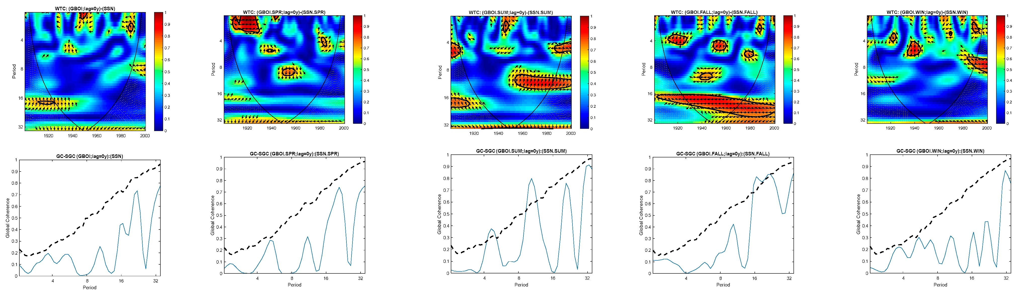
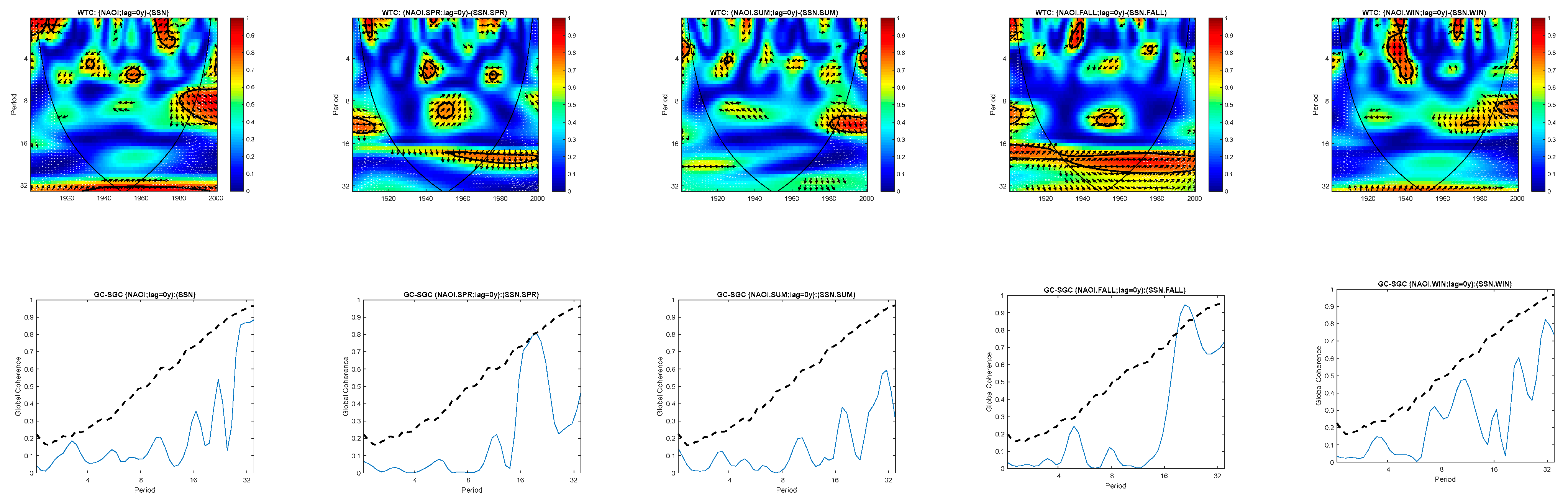
First, we analyzed and discussed the simultaneous links (lag = 0) between the four terrestrial variables and the solar activity quantified by the SSN. The results for the annual averages are shown in the first panel on the left of Figure 1, Figure 2, Figure 3 and Figure 4, with WTC in the upper part and global coherence (GC) in the lower part. The other four panels correspond to the results obtained for the seasonal averages of the terrestrial variables the SSN in the following order from left to right: SPR, SUM, FALL, and WIN.
From the analysis of Figure 1, Figure 2, Figure 3 and Figure 4, it appears that the seasonal analysis provides additional significant information compared to the annual values regarding the relationship between the SSN and the analyzed terrestrial variables. This is most obvious in the cases of the link between the GBOI and SSN (Figure 1) and between the NAOI and SSN (Figure 2), in which the annually averaged time series do not clearly provide any significant coherence. However, the series during the autumn season shows a significant coherence over the entire analysis period of the 20th century, both for the GBOI as well as the NAOI. This significant coherence is related to the influence of the approximately 22-year solar (Hale) cycle. The sign of the link differs from the GBOI to NAOI. This is due to the definition of the two climate indices and the fact that they are negatively correlated. The explanation of this issue exists in the meaning of these two indices in such a way that the NAOI captures the flux of air masses at the level of the land surface in the zonal direction and the GBOI captures the meridional processes. It can be said that the two indices “work” in tandem.
In Figure 1, the arrows pointing from east to west indicate an antiphase between the GBOI and SSN at the 22-year timescale; that is, there is a negative correlation between the GBOI and SSN.
In Figure 2, the NAOI during the autumn season is in phase with the SSN; that is, there is a positive correlation between these variables.
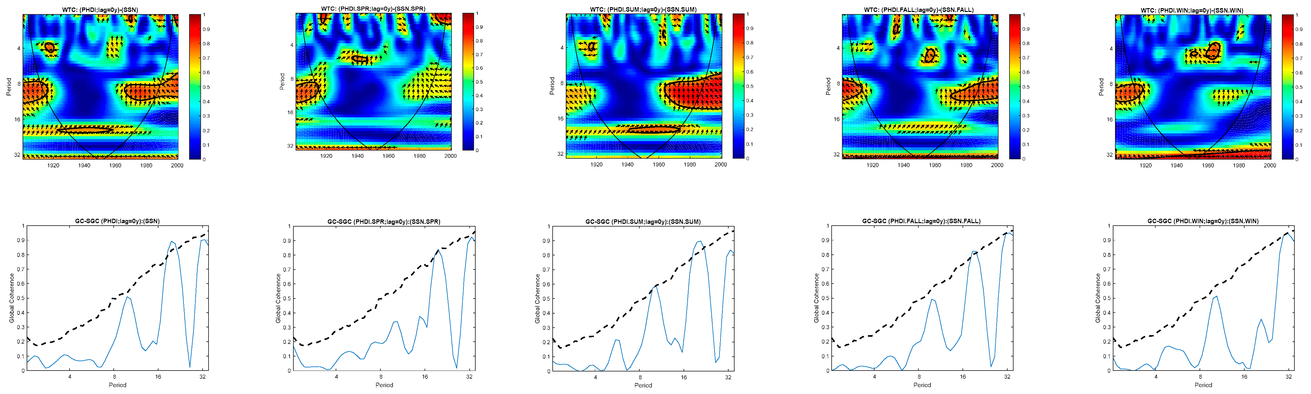
As can be seen in the first panel of Figure 3, for the variable at the regional scale (PHDI), the annual average values of the PHDI have a coherence with the SSN with a statistical significance at a confidence level (CL) that is slightly higher than 95%. This is associated with the solar activity at the Hale solar cycle timescale. It can be observed that this coherence appears more clearly in the summer season compared to the time series considered at the annual level. Here (in the summer season), the highest significance is indicated to occur between 1940 and 1970, as shown by the circled portion inside the cone of influence. Also, in the autumn and winter seasons, a coherence with a CL of 95% can be observed corresponding to the periods of 28–33 years. These are periods that also appear for the annual values but have a slightly lower statistical significance. Regarding the first periodicities associated with the double solar cycle, the arrows on the WTC maps indicate that the variables are in phase, while for the periodicities of approximately 33 years, they are in antiphase. Periods of approximately 33 years are more significant in winter in the second half of the 20th century.
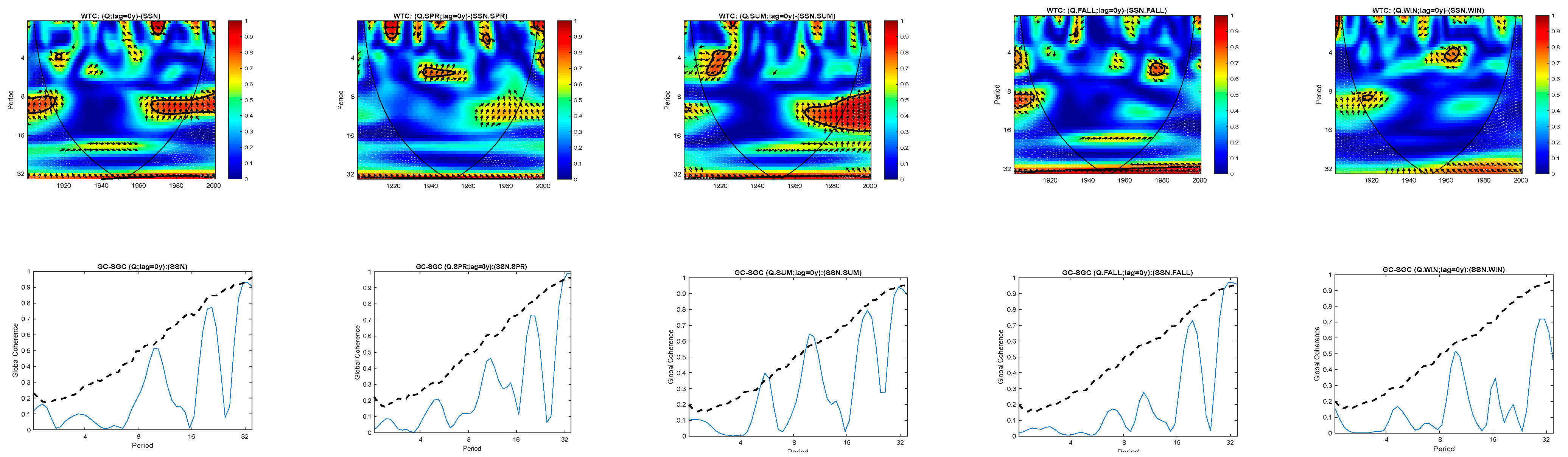
The results of the analysis of the relationship between the SSN and the Danube discharge at Orsova (Q) are presented in Figure 4. Analyzing only the cases in which certain common periodicities appear in coherence between the SSN and Q, as far as possible throughout the analyzed time interval and with the two time series being in phase or antiphase, we have come to the conclusion that only periodicities of approximately 33 years could be considered. Even if most of the values are outside the cone of influence, we will take into account the coherence intensity and the CL of 95% indicated by the global coherence. For the annual values considered simultaneously, the global coherence between the SSN and Q approaches the 95% confidence level (first panel in Figure 4). With a confidence level that is slightly higher than 95%, the coherence values are between the SSN and Q during the spring and autumn seasons. In all cases mentioned above, the two time series are in antiphase.
In addition to this simultaneous analysis between the SSN and the four terrestrial variables described above, we also analyzed the coherence between each of the terrestrial variables and the SSN that were previously considered, with lags of 1–5 years. For the annual values, the lags did not lead to an improvement in the statistical significance of the coherent wavelets.
The results obtained for seasonal average values with lags from 1 to 5 years are presented below, but only for the situations in which the conditions imposed by us in the present study are met; that is, global coherence should have a CL of approximately 95% and the analyzed series should be in phase or antiphase over most of the 100-year time interval analyzed.
Figure 5 shows the evolution of the WTC and GC of the links between the GBOI and SSN from lag 1 and lag 2. It can be seen that at these lags, the links are significant, with a CL slightly higher than 95%, for periodicities, which can be associated with the double solar cycle. At the following lags from 3 to 5 (not shown), the links are insignificant. In the maps representing WTC (left panel in Figure 5), it can be seen that the relationship between the SSN and GBOI in autumn for these periodicities is inverse, with the series being in antiphase. This is especially highlighted at lag 1. It can be interpreted that when the SSN increases, the GBOI values decrease.
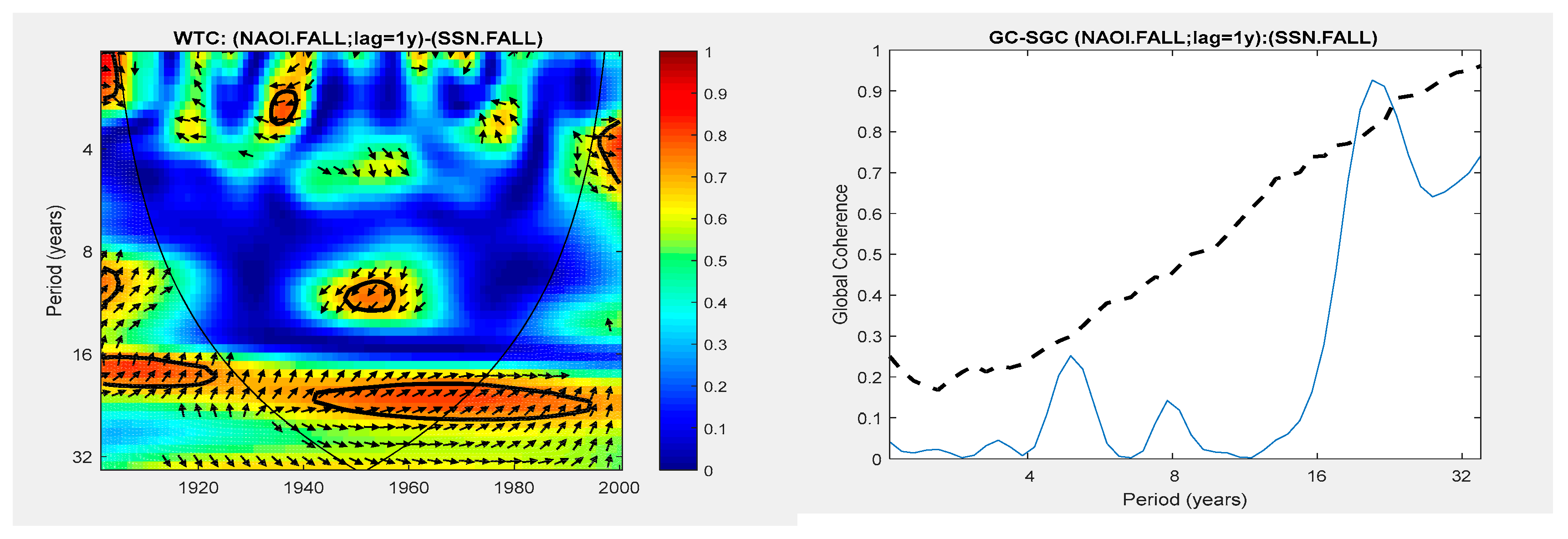
For the NAOI climate index, for the same season (autumn), only one case was found with the imposed conditions regarding the relationship with the SSN with a lag of one year (Figure 6). The significant coherence between the NAOI and SSN is associated with the Hale cycle.
The links are in phase; that is, there are positive correlations between the two variables. If we refer only to the significant coherence inside the cone of influence, in the case of the GBOI, the corresponding area is associated with a larger time interval. However, for the NAOI, this time period is reduced to the interval of 1940–1975.
For example, at the year level, there are no significant coherences for large-scale terrestrial variables. In the autumn season, the SSN associated with the double solar cycle leaves its mark on the NAOI and GBOI, with the coherences being in phase with the NAOI and in antiphase with the GBOI, instead. In other words, high values of the SSN lead to high values of the NAOI and low values of the GBOI.
It seems that for the seasonal average GBOI and NAOI climate indices, the WTC analysis with certain lags provided additional information to allow the variables to be considered simultaneously.
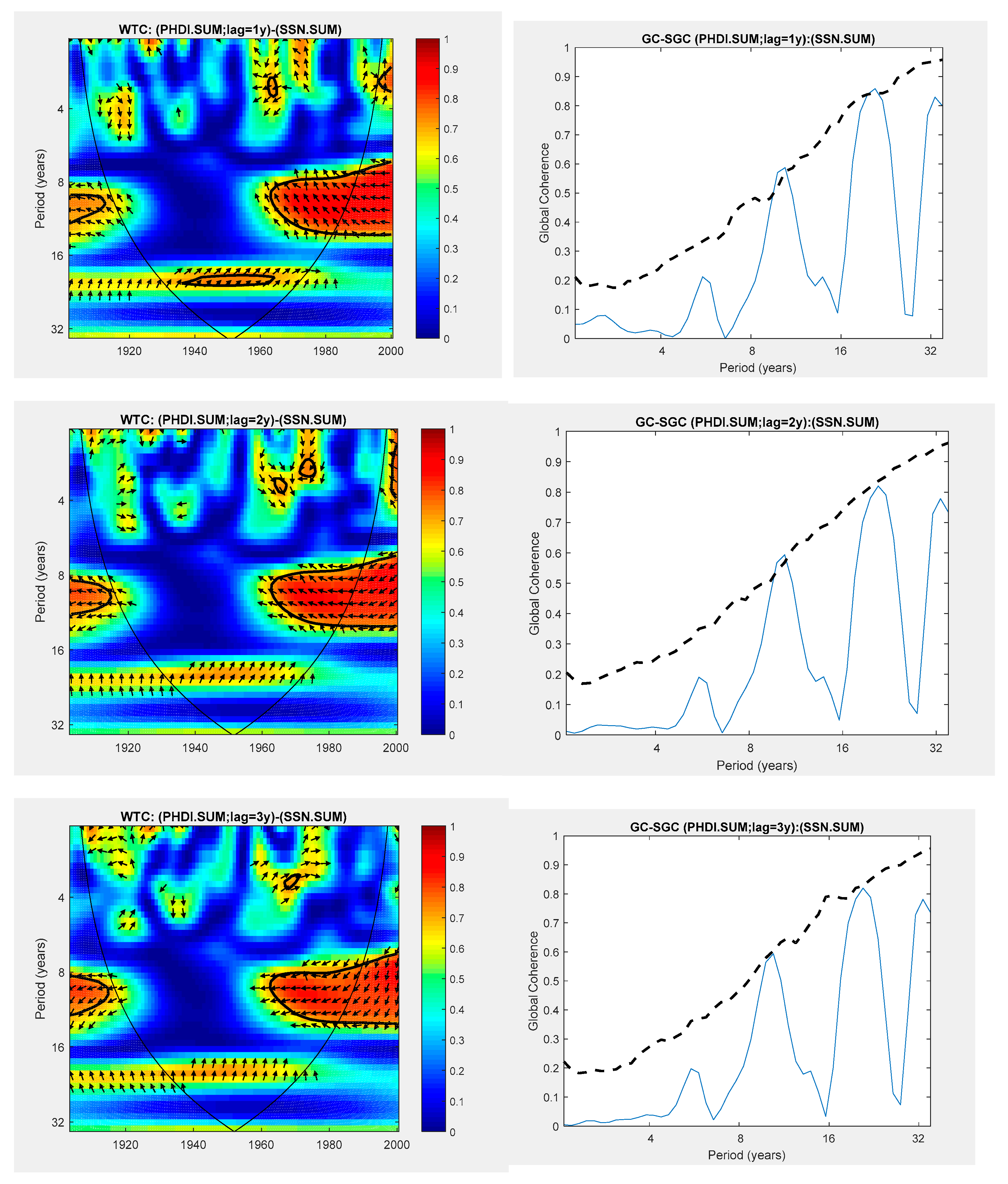
For the variable at the regional scale (PHDI), we chose to present the evolution of the coherence with the SSN at lags from 1 to 3 for the summer season (Figure 7). This choice was related to the fact that in this season, for lag = 0, at the coherences associated with the SSN, the Hale solar cycle timescale meets the requirements that we proposed, namely that they were significant for most of the analyzed 100-year interval and they were in phase or antiphase. Thus, for the SSN associated with cyclicity around the period of 22 years, for the zero lag (simultaneous relations), both the annual values (Figure 3) and those from the summer season have a statistical significance higher than 95%. Regarding the evolution of the coherences between the PHDI and SSN during the summer season with different lags (Figure 7), the periodicity of approximately 22 years (double solar cycle) appears with a significance in close proximity to 95% for lag = 1.
From the analysis of the results presented in Figure 7, a significant global coherence appears instead, with a CL of 95% for periods associated with the Schwabe solar cycle. Although the distribution of the WTC in the panel on the left side of Figure 7 does not show a significant coherence over the entire analyzed time interval, it should be noted that for the beginning of the 20th century and the interval between 1960 and 2000, the coherence between the PHDI and SSN was significant for lags from 1 to 3. The two time series were generally in antiphase in the areas mentioned with significant coherence.
The results regarding the connection between some components of the hydro-climatic system and the solar flux in the second half of the 20th century were analyzed in the study by Mares et al. (2021) [81].
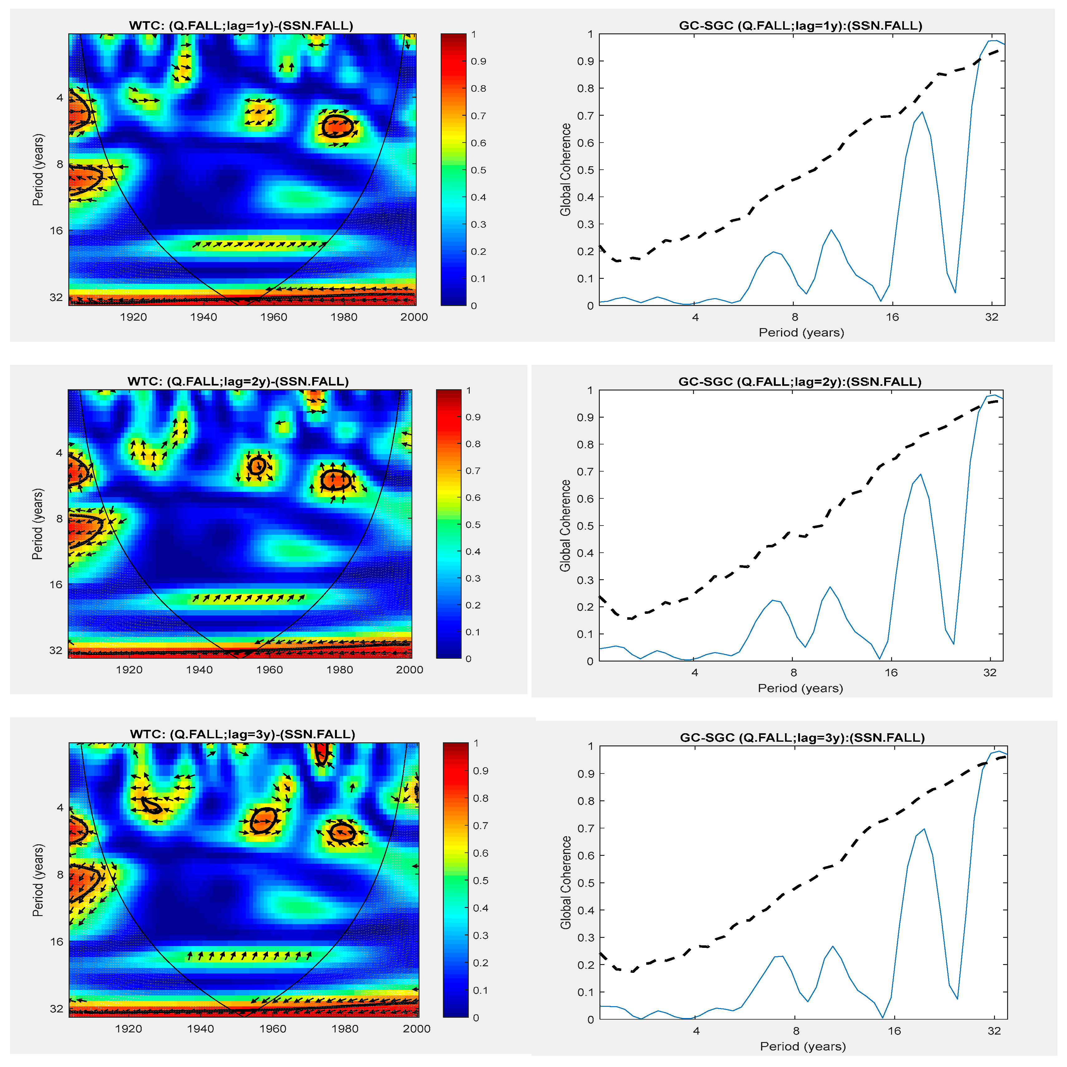
The results regarding the evolution of the connection between the discharge of the Danube at Orsova and the SSN for the fall season (Figure 8) are interesting. If we also analyze the results obtained at lag = 0 (Figure 4), it can be seen that the band of periods (28–33) is almost significant at 95% for the annual averages. Then, in the fall season, it slightly exceeds a 95% CL at lag = 0. Taking into account both WTC (left panel) and GC (right panel), it can be seen that the coherence corresponding to these periods is maintained throughout the 100-year interval analyzed up to lag 3. For period bands 28–33, the Danube discharge in the lower basin was in antiphase with the SSN for lags from 0 to 3.
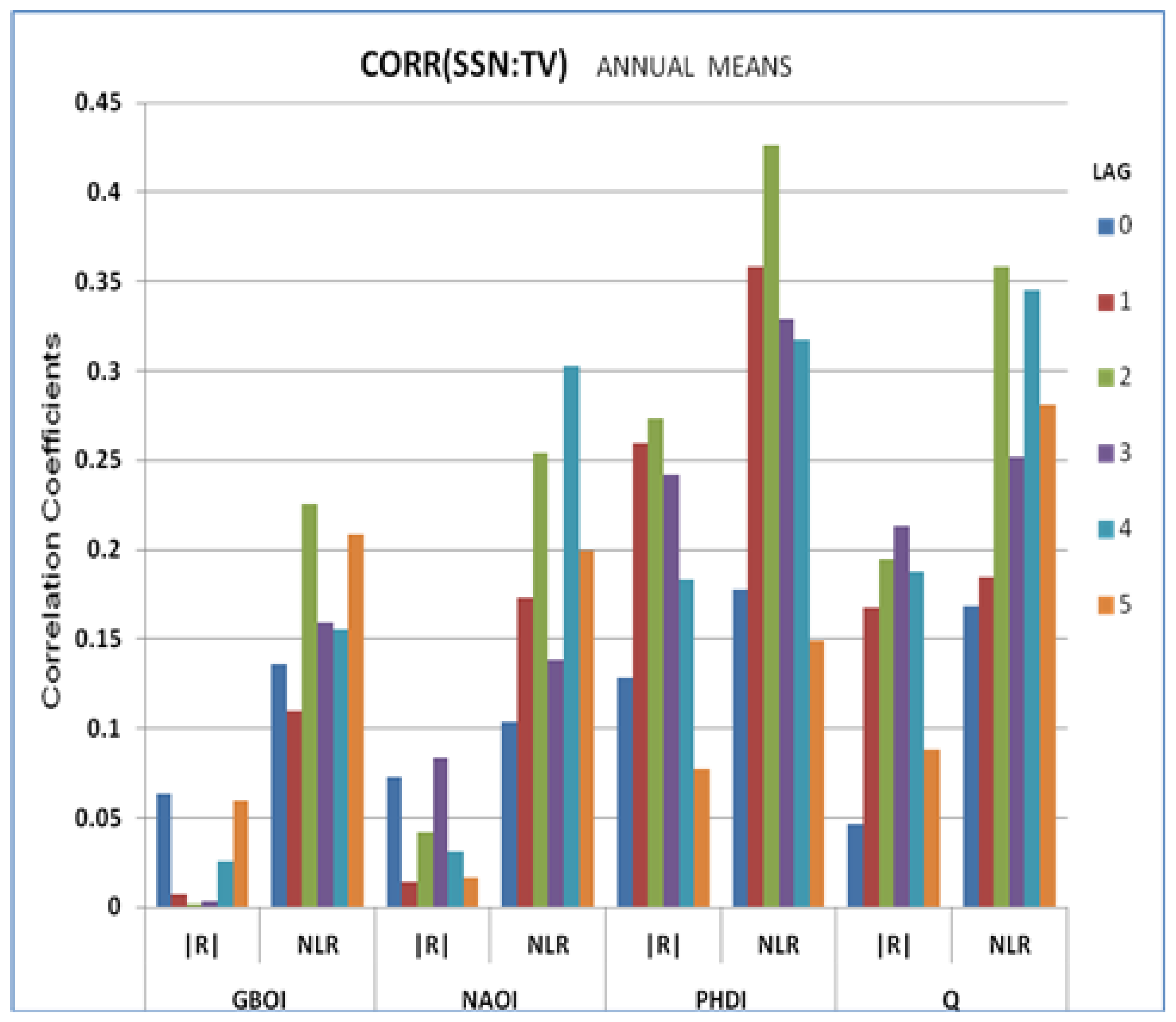
It has been shown previously by the authors in [24,25,26] that the link between the SSN and some of the terrestrial variables considered in this study is non-linear in terms of seasonal average values. Therefore, in the present study, we tested the type of link for the annual values. For this, we calculated the Pearson correlation coefficient (R), which shows a linear relationship between two variables, and the correlation coefficient based on mutual information, called the non-linear correlation coefficient (NLR), calculated according to the relationship (10).
The values of the two correlation coefficients are presented in Figure 9, simultaneously, with lags from 1 to 5 of the SSN before the terrestrial variables. As has been shown in several studies [77,80,83], if NLR > |R|, the relationship between the respective variables is non-linear. As can be seen in Figure 9, for all terrestrial variables considered by annual average values, the relationship with the SSN is non-linear. But we must take into account the statistical significance of these connections. For the size of the data used (100 values), R has a confidence level (CL) of 95% if the value is close to 0.20, while the NLR should be approximately 0.35 for a 95% CL.
In Figure 9, it appears that there is no connection between the large-scale GBOI and NAOI and SSN at a CL of 95%. However, we should still mention that for the NAOI, the SSN from four years prior has an influence at a CL of 90%.
Regarding the climate index at a regional scale (PHDI), the highest NLR was obtained (CL~99%) for the SSN considered 2 years before the PHDI. And for lag 1, the PHDI with the SSN had an NLR with a CL of 95%. It is interesting that the values for R, corresponding to lags 1, 2, and 3, had a CL of 95%. However, since NLR > R, we can consider that the links are non-linear, even in these cases. This was confirmed by the testing carried out, as shown in the Supplementary Information, where Figure S5c proves that this connection is non-linear.
For the discharge of the Danube at Orsova (Q), the variable considered at the local scale, NLR, had a CL of 95% for lag two with the SSN and a CL close to 95% for lag four. The value of R had a CL of 95% in only one case, namely when SSN was considered 3 years before Q.
Such testing to decipher the type of links (linear/non-linear) between variables is of major importance both in the manner of processing the data and in the appropriate interpretations. For this reason, this analysis is somehow proved by the considerations presented in the Supplementary Information [66,72,79,84,85,86,87,88,89,90,91,92,93,94,95]. In Figures S1–S3 and S5, it can be seen that these relationships are non-linear, especially where the connections of terrestrial variables with the SSN were tested.
3.2. Atmospheric and Solar Activity Forcings on the Danube Discharge
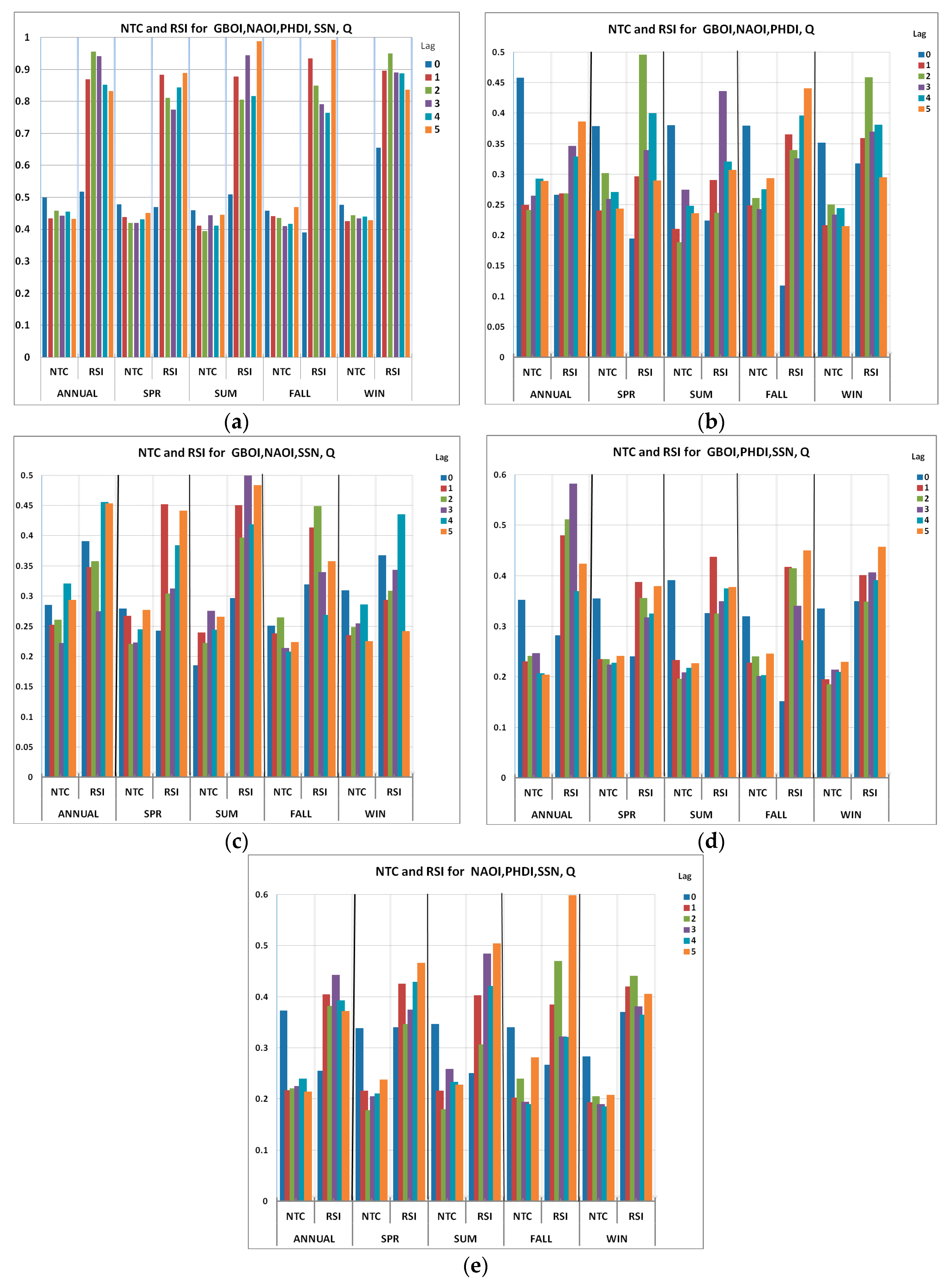
As was mentioned previously, the combined effects of the atmospheric and solar activity forcings on the Danube discharge were achieved using the normalized total correlation and redundancy–synergy index. The results, taking the effects of various combinations of atmospheric and solar forcings on the Danube discharge into consideration, are presented in Figure 10. In order to provide synergistic information for the predictor variables in the case of a considered predictand, the value of the RSI must be positive and have a value as high as possible. The RSI is negative when the predictor variables provide redundant information regarding the predictand; the higher the RSI, the lower the redundancy.
Accordingly, the cases when the NTC has relatively high values compared to other values in the same set and when the RSI has the highest values will be discussed. Two cases were analyzed:
- I.
- Analysis of the information provided for Q by four predictors together (GBOI, NAOI, PHDI, and SSN) for annual and seasonal values (Figure 10a);
- II.
- The analysis provided for Q of three predictors under different combinations, namely:
- (a)
- Terrestrial variables (GBOI, NAOI, PHDI) (Figure 10b);
- (b)
- The two large-scale terrestrial variables (GBOI, NAOI) together with the SSN (Figure 10c);
- (c)
- One variable at a large scale (GBOI) and one at a regional scale (PHDI) with the SSN (Figure 10d);
- (d)
- The same as (c) but with the NAOI instead of the GBOI (Figure 10e).
In all cases, the results are presented for the annual and seasonal values with lags from 0 (simultaneous) to 5 years between the predictors and the predictand Q.
It can be observed that for case I, the set consisting of all four variables considered predictors (Figure 10a), the RSI values were high. Therefore, there was a synergistic action for both annual and seasonal values for lags from 1 to 5 years. Regarding the simultaneous information, even if the NTC has higher values than those corresponding to lags (except for autumn), the RSI has relatively low values, and it appears that there is a redundancy of the predictor variables.
Now, we will discuss the results from point II. Figure 10b shows the results by considering only the terrestrial predictors (GBOI, NAOI, and PHDI). For the predictors considered simultaneously with the predictand, no significant results were observed because even if the NTC had higher values (especially for the annual values), the RSI values were relatively low.
If we refer to the results with lags from 1 to 5 years, the value of the RSI during the spring was noted at lag 2, which also corresponded to the relatively high value of the NTC. The results from the winter season were also at the same lag. We can also mention the results from lag 3 (summer) and lag 5 (autumn), taking into account the comparison of the RSI with the NTC.
In the following cases, a terrestrial predictor was replaced by the SSN. Thus, Figure 10c shows the results of the combination between the SSN, GBOI, and NAOI. For this situation, we have mentioned the most significant result, which was obtained in the summer season at lag 3.
When the combination of three predictors (two terrestrial, of which the PHDI was a part) was introduced in combination with the GBOI, the results were the most remarkable for the annual values at lag 3 (Figure 10d).
For the last variant of combining the predictors (NAOI, PHDI, and SSN), the results are shown in Figure 10e. If we take into account both the values of the NTC and RSI, we can see the agreement between the two indices for lag 3 summer and lag 5 autumn.
The results obtained using this approach will be used for the consideration/selection of predictors for estimating the Danube discharge in the lower basin through the optimal combination of terrestrial variables with those describing the variability of solar activity.
The ranking of the predictors according to the synergistic contribution to the predictand is essential for the type of relationship used in the practice of extrapolation and for estimating the discharge of the Danube in the lower basin. This investigation will be the subject of a future study.
4. Conclusions
The influence of solar activity on the Southeastern European climate at different spatio-temporal scales was tested using global coherence (GC). This highlighted the significant periodicities averaged over the analyzed time interval. In addition, wavelet coherence (WTC) was also employed, which provides details in the time–frequency domain.
By imposing certain assumptions regarding the achieved results, namely the discussion of those in which the SSN is in phase or antiphase with the terrestrial variables and those with lags from 0 to 5 years, it emerged that the analysis on seasonal averages provided additional significant information compared to the annual averages. Accordingly, for the large-scale climate indices, the GBOI and NAOI were at the level of the annual average values, and no coherence with the solar activity was evident at a statistical significance greater than or close to 95%. Instead, a significant coherence clearly appeared between the solar activity and the two climatic indices at the 22-year (Hale) solar cycle timescale for the autumn season at lag = 0 and lag = 1 year.
The Hale solar cycle, in the case of the PHDI, is present in the annual and summer season averages and more clearly at lag = 0. For the Danube discharge at Orsova, the most significant SSN signature (~95%) was observed at periods of 33 years in the autumn season for lags from 0 to 3 years.
For the variable at the regional scale (PHDI), the average annual values of the PHDI have a coherence with the SSN at lag = 0, with a statistical significance slightly higher than 95%, which is associated with the Hale solar cycle. This coherence appears more clearly in the summer season compared to the time series considered at the annual level. In the autumn and winter seasons, at lag = 0, a coherence with a 95% CL could be observed, especially at the GC. This corresponded to the period of 28–33 years. This time period also appeared at the level of the annual values but with a slightly lower statistical significance. For the first periodicities associated with the double solar cycle, the variables were in phase, while for the cycle of approximately 33 years, they were in antiphase.
From the analysis of the relationship between the SSN and the Danube discharge at Orsova (Q), only periodicities of approximately 33 years (Brüuckner cycle) were significant at lag = 0 in terms of annual averages, taking into account the imposed conditions. Here, the global coherence between the SSN and Q approached a 95% confidence level. With a confidence level slightly higher than 95%, the coherence values between the SSN and Q during the autumn season, at lags from 0 to 3, were observed for the periodicities around 30 years. In all cases mentioned above, the two time series were in antiphase.
On testing the nature of the links using mutual information, it emerged that the link with the SSN was non-linear when the annual average values were considered for all terrestrial variables. This was similar to that of the seasonal variables.
In conclusion, with certain conditions imposed (namely, only the results for which the coherences between the SSN and the terrestrial variables were in phase or antiphase and significant for almost the entire 20th century), only certain periodicities associated with the double solar cycle and a periodicity of around 30 years were highlighted in this study.
Although certain time interval periodicities associated with the Schwabe cycle were significant (especially summer for PHDI), they were not detailed in the present study due to them being studied in a future investigation. This future investigation will take into account the characteristics of the respective 11-year cycles related to their intensity and duration and the behavior of terrestrial variables at certain stages of the development of these solar cycles on the ascending or descending slope.
With the aim of finding the best synergistic combination for estimating the Danube discharge in the lower basin, through the optimal combination of terrestrial variables with those describing the solar activity variability, multivariate analysis concepts, such as the normalized total correlation and the redundancy–synergy index, were applied. The results showed that this synergistic combination depends on both the timescale and solar activity.
For example, the annual average values among the three possible combinations of atmospheric predictors with the solar variable of the SSN were evaluated. The most significant result with a high synergetic index was obtained in the case of the combination of terrestrial variables, the GBOI and PHDI, with the SSN, considered 3 years before the discharge of the Danube at Orsova.
Regarding the seasonal values, the highest synergetic index was obtained for the combination of predictors (NAOI, PHDI, SSN) in the autumn season, with a lag of 5 years compared to Q.
The ranking of the predictors according to the synergistic contribution to the predictand is essential in terms of the type of relationship used for extrapolation when estimating the discharge of the Danube in the lower basin. This will be the subject of a future study.
Supplementary Materials
The following supporting information can be downloaded at https://www.mdpi.com/article/10.3390/atmos14111622/s1, Figure S1: Relationship between (a) the PHDI (X1) and SSN (X2); (b) the PHDI (X1) and Q (X3); (c) the SSN (X2) and Q (X3); (d) the spatial representation of the overall combination of the three variables in the spring season. The blue points are the data, and those shown by a curve made up of red small circles are a kind of fit of the data; Figure S2: Same variables as in Figure S1 but for the summer season; Figure S3: Relationship between the GBOI (X1), PHDI (X2), and Q (X3) during the spring season; Figure S4: Relationship between the GBOI (X1), PHDI (X2), and Q (X3) for annual values; Figure S5: Relationship between the Q (X1), SSN (X2), and PHDI (X3) for annual values.
Author Contributions
Conceptualization, I.M.; investigation, I.M, C.M., and V.D.; methodology, C.M., I.M., and V.D.; writing—original draft preparation, I.M., V.D., C.M., and C.D.; supervision and validation, C.D. All authors have read and agreed to the published version of the manuscript.
Funding
This research received no external funding.
Institutional Review Board Statement
Not applicable.
Informed Consent Statement
Not applicable.
Data Availability Statement
The NAOI data are available from the Climate Research Unit (https://crudata.uea.ac.uk/cru/data/nao/values.htm, accessed on 9 February 2023). The SSN data are available from WDC-SILSO, Royal Observatory of Belgium, Brussels (http://www.sidc.be/silso/datafiles, accessed on 9 February 2023). The GBOI data presented in this study are available on request from the corresponding author. The GBOI data is not available due to restrictions. Danube discharge at Orsova (Q) are provided by the National Institute of Hydrology and Water Management, Bucharest, Romania.
Conflicts of Interest
The authors declare no conflict of interest.
References
- Peng, T.; Zhou, J.; Zhang, C.; Fu, W. Streamflow Forecasting Using Empirical Wavelet Transform and Artificial Neural Networks. Water 2017, 9, 406. [Google Scholar] [CrossRef]
- Weijs, S.V.; Foroozand, H.; Kumar, A. Dependency and redundancy: How information theory untangles three variable interactions in environmental data. Water Resour. Res. 2018, 54, 7143–7148. [Google Scholar] [CrossRef]
- Serykh, I.V.; Sonechkin, D.M. El Niño–Global Atmospheric Oscillation as the Main Mode of Interannual Climate Variability. Atmosphere 2021, 12, 1443. [Google Scholar] [CrossRef]
- Daglis, I.A.; Chang, L.C.; Dasso, S.; Gopalswamy, N.; Khabarova, O.V.; Kilpua, E.; Lopez, R.; Marsh, D.; Matthes, K.; Nandy, D.; et al. Predictability of variable solar–terrestrial coupling. Ann. Geophys. 2021, 39, 1013–1035. [Google Scholar] [CrossRef]
- Dobrica, V.; Demetrescu, C. Oscillations at sub-centennial time scales in the space climate of the last 150 years. Rev. Roum. Géophysique 2021, 65, 71–77. [Google Scholar] [CrossRef]
- Demetrescu, C.; Dobrica, V.; Maris, G. On the long-term variability of the heliosphere—Magnetosphere environment. Adv. Space Res. 2010, 46, 1299–1312. [Google Scholar] [CrossRef]
- Dobrica, V.; Demetrescu, C.; Maris, G. On the response of the European climate to the solar/geomagnetic long-term activity. Ann. Geophys. 2010, 53, 39–48. [Google Scholar]
- Le Mouël, J.L.; Lopes, F.; Courtillot, V. A solar signature in many climate indices. J. Geoph. Res. Atmos. 2019, 124, 2600–2619. [Google Scholar] [CrossRef]
- Eyring, V.; Bony, S.; Meehl, G.A.; Senior, C.A.; Stevens, B.; Stouffer, R.J.; Taylor, K.E. Overview of the Coupled Model Intercomparison Project phase 6 (CMIP6) experimental design and organization. Geosci. Model Dev. 2016, 9, 1937–1958. [Google Scholar] [CrossRef]
- Roy, I. Solar cyclic variability can modulate winter Arctic climate. Sci. Rep. 2018, 8, 4864. [Google Scholar] [CrossRef]
- Zhao, R.; Biswas, A.; Zhou, Y.; Zhou, Y.; Shi, Z.; Li, H. Identifying localized and scale-specific multivariate controls of soil organic matter variations using multiple wavelet coherence. Sci. Total Environ. 2018, 643, 548–558. [Google Scholar] [CrossRef]
- Chham, E.; Milena-Pérez, A.; Piñero-García, F.; Hernández-Ceballos, M.A.; Orza, J.A.; Brattich, E.; El Bardouni, T.; Ferro-García, M.A. Sources of the seasonal-trend behaviour and periodicity modulation of 7Be air concentration in the atmospheric surface layer observed in southeastern Spain. Atmos. Environ. 2019, 15, 148–158. [Google Scholar] [CrossRef]
- Salvadori, G.; De Michele, C.; Kottegoda, N.; Rosso, R. Extremes in Nature: An Approach Using Copulas. In Water Science and Technology Library; Springer: Dordrecht, The Netherlands, 2007; Volume 56. [Google Scholar]
- Sonechkin, D.M.; Vakulenko, N.V. Polyphony of Short-Term Climatic Variations. Atmosphere 2021, 12, 1145. [Google Scholar] [CrossRef]
- Ianovici, V.; Mihailescu, V.; Badea, L.; Moraru, T.; Tufescu, V.; Iancu, M.; Herbst, C.; Grumazescu, H. Geografia Vaii Dunarii romanesti. Ed. Acad. Republicii Social. Rom. 1969, 2, 782. [Google Scholar]
- Stănescu, V.A.; Ungureanu, V.; Domokos, M. Regionalization of the Danube catchment for the estimation of the distribution functions of annual peak discharges. J. Hydrol. Hydromech. 2001, 49, 407–427. [Google Scholar]
- Stănescu, V.A. Regional Analysis of The Annual Peak Discharges in the Danube Catchment; Follow–up volume No.VII to the Danube Monograph. Regional Cooperation of the Danube Countries; Administrația Națională de Meteorologie: Bucharest, Romania, 2004; p. 64. [Google Scholar]
- Pekarova, P.; Pekar, J. Long-term discharge prediction for the Turnu Severin station (the Danube) using a linear autoregressive model. Hydrol. Process. 2006, 20, 1217–1228. [Google Scholar] [CrossRef]
- Rimbu, N.; Dima, M.; Lohmann, G.; Stefan, S. Impacts of the North Atlantic Oscillation and the El Niño–Southern Oscillation on Danube river flow variability. Geophys. Res. Lett. 2004, 31, L23203. [Google Scholar] [CrossRef]
- Dobrica, V.; Demetrescu, C.; Mares, I.; Mares, C. Long-term evolution of the Lower Danube discharge and corresponding climate variations: Solar signature imprint. Theor. Appl. Climatol. 2018, 133, 985–996. [Google Scholar] [CrossRef]
- Pekárová, P.; Miklánek, P. (Eds.) Flood Regime of Rivers in the Danube River Basin; Follow–up volume IX of the Regional Co-operation of the Danube Countries in IHP UNESCO; IH SAS: Bratislava, Slovakia, 2019; Volume 215, p. 527. [Google Scholar] [CrossRef]
- Mares, I.; Dobrica, V.; Demetrescu, C.; Mares, C. Hydrological response in the Danube lower basin to some internal and external climate forcing factors. Hydrol. Earth. Syst. Sci. Discuss. 2016, preprint. [Google Scholar]
- Mares, C.; Mares, I.; Mihailescu, M. Identification of extreme events using drought indices and their impact on the Danube lower basin discharge. Hydrol. Process. 2016, 30, 3839–3854. [Google Scholar] [CrossRef]
- Mares, I.; Mares, C.; Dobrica, V.; Demetrescu, C. Comparative study of statistical methods to identify a predictor for discharge at Orsova in the Lower Danube Basin. Hydrol. Sci. J. 2020, 65, 371–386. [Google Scholar] [CrossRef]
- Mares, I.; Dobrica, V.; Mares, C.; Demetrescu, C. Assessing the solar variability signature in climate variables by information theory and wavelet coherence. Sci. Rep. 2021, 11, 11337. [Google Scholar] [CrossRef] [PubMed]
- Mares, I.; Mares, C.; Dobrica, V.; Demetrescu, C. Selection of Optimal Palmer Predictors for Increasing the Predictability of the Danube Discharge: New Findings Based on Information Theory and Partial Wavelet Coherence Analysis. Entropy 2022, 24, 1375. [Google Scholar] [CrossRef] [PubMed]
- Mares, C.; Mares, I.; Dobrica, V.; Demetrescu, C. Discriminant Analysis of the Solar Input on the Danube’s Discharge in the Lower Basin. Atmosphere 2023, 14, 1281. [Google Scholar] [CrossRef]
- Scafetta, N. Global temperatures and sunspot numbers. Are they related? Yes, but non linearly. A reply to Gil-Alana et al. (2014). Phys. A Stat. Mech. Appl. 2014, 413, 329–342. [Google Scholar] [CrossRef]
- Halberg, F.; Cornélissen, G.; Bernhardt, K.H.; Sampson, M.; Schwartzkopff, O.; Sonntag, D. Egeson’s (George’s) transtridecadal weather cycling and sunspots. Hist. Geo Space Sci. 2010, 1, 49–61. [Google Scholar] [CrossRef]
- Zhao, J.; Han, Y.-B.; Li, Z.-A. The effect of solar activity on the annual precipitation in the Beijing area. Chinese J. Astron. Astroph. 2004, 4, 189–197. [Google Scholar] [CrossRef]
- Dobrica, V.; Demetrescu, C.; Boroneant, C.; Maris, G. Solar and geomagnetic activity effects on climate at regional and global scales: Case study—Romania. J. Atmos. Solar-Terrestr. Phys. 2009, 71, 1727–1735. [Google Scholar] [CrossRef]
- Mauas, P.J.D.; Buccino, A.P.; Flamenco, E. Long-term solar activity influences on South american rivers. J. Atmos. Sol. Terr. Phys. 2011, 73, 377–382. [Google Scholar] [CrossRef]
- Briciu, A.-E.; Mihaila, D. Wavelet analysis of some rivers in SE Europe and selected climate indices. Environ. Monit. Assess. 2014, 186, 6263–6286. [Google Scholar] [CrossRef]
- Compagnucci, R.H.; Berman, A.L.; Herrera, V.V.; Silvestri, G. Are southern South American Rivers linked to the solar variability? Int. J. Clim. 2014, 34, 1706–1714. [Google Scholar] [CrossRef]
- Sunkara, S.L.; Tiwari, R.K. Wavelet analysis of the singular spectral reconstructed time series to study the imprints of solar–ENSO–geomagnetic activity on Indian climate. Nonlin. Processes Geoph. 2016, 23, 361–374. [Google Scholar] [CrossRef]
- Matveev, S.M.; Chendev, Y.G.; Lupo, A.R.; Hubbart, J.A.; Timashchuk, D.A. Climatic Changes in the East-European Forest-Steppe and Effects on Scots Pine Productivity. Pure Appl. Geophys. 2017, 174, 427–443. [Google Scholar] [CrossRef]
- Laurenz, L.; Lüdecke, H.J.; Lüning, S. Influence of solar activity changes on European rainfall. J. Atmos. Sol. Terr. Phys. 2019, 185, 29–42. [Google Scholar] [CrossRef]
- Bierkens, M.F.P.; van Beek, L.P.H. Seasonal Predictability of European Discharge: NAO and Hydrological Response Time. J. Hydrometeor. 2009, 10, 953–968. [Google Scholar] [CrossRef]
- Su, L.; Miao, C.; Duan, Q.; Lei, X.; Li, H. Multiple-wavelet coherence of world’s large rivers with meteorological factors and ocean signals. J. Geoph. Res. Atmos. 2019, 124, 4932–4954. [Google Scholar] [CrossRef]
- Dai, Z.J.; Du, J.Z.; Tang, Z.H.; Ou, S.Y.; Brody, S.; Mei, X.F.; Jing, J.T.; Yu, S.B. Detection of Linkage Between Solar and Lunar Cycles and Runoff of the World’s Large Rivers. Earth Space Sci. 2019, 6, 914–930. [Google Scholar] [CrossRef]
- Ballinger, A.P.; Schurer, A.P.; O’Reilly, C.H.; Hegerl, G.C. The importance of accounting for the North Atlantic Oscillation when applying observational constraints to European climate projections. Geophys. Res. Lett. 2023, 50, e2023GL103431. [Google Scholar] [CrossRef]
- Bednorz, E.; Czernecki, B.; Tomczyk, A.M.; Półrolniczak, M. If not NAO then what?—Regional circulation patterns governing summer air temperatures in Poland. Theor. Appl. Climatol. 2019, 136, 1325–1337. [Google Scholar] [CrossRef]
- Hurrell, J.W. Decadal trends in the North Atlantic oscillation:Regional temperatures and precipitation. Science 1995, 269, 676–679. [Google Scholar] [CrossRef]
- Ambaum, M.H.P.; Hoskins, B.J.; Stephenson, D.B. Arctic Oscillation or North Atlantic Oscillation? J. Clim. 2001, 14, 3495–3507. [Google Scholar] [CrossRef]
- Mares, I.; Mares, C.; Stanciu, P. Climate Variability of the Discharge Level in the Danube Lower Basin and Teleconnection with NAO. Conference on Water Observation and Information System for Decision Support, Balwois. 2006. Available online: https://balwois.com/wp-content/uploads/old_proc/ffp-672.pdf (accessed on 1 September 2023).
- Mares, I.; Mares, C.; Mihailescu, M. NAO impact on the summer moisture variability across Europe. Phis. Chem. Earth. 2002, 27, 1013–1017. [Google Scholar] [CrossRef]
- Folland, C.K.; Knight, J.; Linderholm, H.W.; Fereday, D.; Ineson, S.; Hurrell, J.W. The summer North Atlantic oscillation: Past, present, and future. J. Clim. 2009, 22, 1082–1103. [Google Scholar] [CrossRef]
- Bladé, I.; Liebmann, B.; Fortuny, D.; van Oldenborgh, G.J. Observed and simulated impacts of the summer NAO in Europe: Implications for projected drying in the Mediterranean region. Clim. Dyn. 2012, 39, 709–727. [Google Scholar] [CrossRef]
- Mellado-Cano, J.; Barriopedro, D.; García-Herrera, R.; Trigo, R.M. New observational insights into the atmospheric circulation over the Euro-Atlantic sector since 1685. Clim. Dyn. 2020, 54, 823–841. [Google Scholar] [CrossRef]
- Lled_o, L.; Cionni, I.; Torralba, V.; Bretonni_ere, P.-A.; Sams_o, M. Seasonal prediction of Euro-Atlantic teleconnections from multiple systems. Environ. Res. Lett. 2020, 15, 074009. [Google Scholar] [CrossRef]
- Mares, I.; Mares, C.; Mihailescu, M. Stochastic modeling of the connection between sea level pressure and discharge in the Danube lower basin by means of Hidden Markov Model. EGU Gen. Assem. Conf. Abstr. 2013, 15, 7606. [Google Scholar]
- Yin, Z.Y. Spatial pattern of temporal trends in moisture conditions in the southeastern United States. Geogr. Ann. Ser. A Phys. Geogr. 1993, 75, 1–11. [Google Scholar] [CrossRef]
- Loboda, N.S.; Bozhok, Y.V. Electronic book with full papers. In Proceedings of the XXVIIІ Conference of the Danubian Countries on Hydrological Forecasting and Hydrological Bases of Water Management, Kyiv, Ukraine, 6–8 November 2019. [Google Scholar]
- Nakicenovic, N.; Alcamo, J.; Grubler, A.; Riahi, K.; Roehrl, R.A.; Rogner, H.-H.; Victor, N. Special Report on Emissions Scenarios (SRES), A Special Report of Working Group III of the Intergovernmental Panel on Climate Change; Cambridge University Press: Cambridge, UK, 2000; ISBN 0-521-80493-0. [Google Scholar]
- Wu, Y.; Zhang, L.; Zhang, Z.; Ling, J.; Yang, S.; Si, J.; Zhan, H.; Chen, W. Influence of solar activity and large-scale climate phenomena on extreme precipitation events in the Yangtze River Economic Belt. Stoch. Env. Res. Risk Assess. 2023. [Google Scholar] [CrossRef]
- Tomasino, M.; Zanchettin, D.; Traverso, P. Long-range forecastsof River Po discharges based on predictable solar activity and a fuzzy neural network model. Hydrol. Sci. J. 2004, 49, 673–684. [Google Scholar] [CrossRef]
- Landscheidt, T. River Po discharges and cycles of solar activity. Hydrol. Sci. J. 2000, 45, 491–493. [Google Scholar] [CrossRef]
- Wrzesiński, D.; Sobkowiak, L.; Mares, I.; Dobrica, V.; Mares, C. Variability of River Runoff in Poland and Its Connection to Solar Variability. Atmosphere 2023, 14, 1184. [Google Scholar] [CrossRef]
- Zanchettin, D.; Rubino, A.; Traverso, P.; Tomasino, M. Impact of variations in solar activity on hydrological decadal patterns in northern Italy. J. Geophys. Res. 2008, 13, 889. [Google Scholar] [CrossRef]
- Massei, N.; Laignel, B.; Deloffre, J.; Mesquita, J.; Motelay, A.; Lafite, R.; Durand, A. Long-term hydrological changes of the Seine River flow (France) and their relation to the North Atlantic Oscillation over the period 1950–2008. Int. J. Clim. 2010, 30, 2146–2154. [Google Scholar] [CrossRef]
- Fu, C.; James, A.L.; Wachowiak, M.P. Analyzing the combined influence of solar activity and El Niño on streamflow across southern Canada. Water Resour. Res. 2012, 48, W05507. [Google Scholar] [CrossRef]
- Antico, A.; Torres, M.E. Evidence of a decadal solar signal in the Amazon River: 1903 to 2013. Geophys. Res. Lett. 2015, 42, 782–787. [Google Scholar] [CrossRef]
- Dong, L.; Fu, C.; Liu, J.; Zhang, P. Combined Effects of Solar Activity and El Niño on Hydrologic Patterns in the Yoshino River Basin, Japan. Water Resour. Manag. 2018, 32, 2421. [Google Scholar] [CrossRef]
- Torrence, C.; Compo, G.P. A Practical Guide to Wavelet Analysis. Bull. Am. Meteorol. Soc. 1998, 79, 61–78. [Google Scholar] [CrossRef]
- Grinsted, A.; Moore, J.C.; Jevrejeva, S. Application of the cross wavelet transform and wavelet coherence to geophysical time series. Nonlinear Process. Geophys. 2004, 11, 561–566. [Google Scholar] [CrossRef]
- Moore, J.; Grinsted, A.; Jevrejeva, S. Is there evidence for sunspot forcing of climate at multi-year and decadal periods? Geophys. Res. Lett. 2006, 33, L17705. [Google Scholar] [CrossRef]
- Schulte, J.; Najjar, R.G.; Li, M. The influence of climate modes on streamflow in the Mid-Atlantic region of the United States. J. Hydrol. Reg. Stud. 2016, 5, 80–99. [Google Scholar] [CrossRef]
- Shannon, C.E. A mathematical theory of communication. Bell Syst. Tech. J. 1948, 27, 379–423. [Google Scholar] [CrossRef]
- Guiasu, S. Information Theory with Applications; McGraw-Hill Inc.: London, UK, 1977. [Google Scholar]
- Timme, N.; Alford, W.; Flecker, B.; Beggs, J.M. Synergy, redundancy, and multivariate information measures: An experimentalist’s perspective. J. Comput. Neurosci. 2014, 36, 119–140. [Google Scholar] [CrossRef] [PubMed]
- Ball, K.R.; Grant, C.; Mundy, W.R.; Shafer, T.J. A multivariate extensionof mutual information for growing neural networks. Neural Netw. 2017, 95, 29–43. [Google Scholar] [CrossRef] [PubMed]
- Timme, N.M.; Lapish, C. A tutorial for information theory in neuroscience. Eneuro 2018, 5, 1–40. [Google Scholar] [CrossRef]
- Hsieh, W.W.; Tang, B. Applying neural network models to prediction and data analysis in meteorology and oceanography. Bull. Am. Meteorol. Soc. 1998, 79, 1855–1870. [Google Scholar] [CrossRef]
- Schulte, J. Global Wavelet Coherence, MATLAB Central File Exchange. Available online: https://www.mathworks.com/matlabcentral/fileexchange/54682-global-wavelet-coherence (accessed on 9 February 2023).
- Hu, W.; Si, B.C. Technical Note: Multiple wavelet coherence for untangling scale-specific and localized multivariate relationships in geosciences. Hydrol. Earth Syst. Sci. 2016, 20, 3183–3191. [Google Scholar] [CrossRef]
- Hu, W.; Si, B.C. Technical Note: Improved partial wavelet coherency for understanding scale-specific and localized bivariate relationships in geosciences. Hydrol. Earth Syst. Sci. 2021, 25, 321–331. [Google Scholar] [CrossRef]
- Khan, S.; Ganguly, A.R.; Bandyopadhyay, S.; Saigal, S.; Erickson III, D.J.; Protopopescu, V.; Ostrouchov, G. Nonlinear statistics reveals stronger ties between ENSO and the tropical hydrological cycle. Geophys. Res. Lett. 2006, 33, L24402. [Google Scholar] [CrossRef]
- Wrzesiński, D. Uncertainty of flow regime characteristics of rivers in Europe. Quaest. Geogr. 2013, 32, 43–53. [Google Scholar] [CrossRef]
- Gong, W.; Yang, D.; Gupta, H.V.; Nearing, G. Estimating information entropy for hydrological data: One-dimensional case. Water Res. 2014, 50, 5003–5018. [Google Scholar] [CrossRef]
- Vu, T.M.; Mishra, A.K.; Konapala, G. Information Entropy Suggests Stronger Nonlinear Associations between Hydro-Meteorological Variables and ENSO. Entropy 2018, 20, 38. [Google Scholar] [CrossRef] [PubMed]
- Mares, C.; Mares, I.; Dobrica, V.; Demetrescu, C. Quantification of the direct solar impact on some components of the hydroclimatic system. Entropy 2021, 23, 691. [Google Scholar] [CrossRef]
- Smith, R. A Mutual Information Approach to Calculating Nonlinearity. Stat 2015, 4, 291–303. [Google Scholar] [CrossRef]
- Yoon, S.; Lee, T. Investigation of hydrological variability in the Korean Peninsula with the ENSO teleconnections. Proc. Int. Assoc. Hydrol. Sci. 2016, 374, 165–173. [Google Scholar] [CrossRef]
- Hotelling, H. Relations Between Two Sets of Variates. Biometrika 1936, 28, 321–377. [Google Scholar] [CrossRef]
- Lorenz, E.N. Empirical orthogonal functions and statistical weather prediction. In Statistical Forecasting Project; Department of Meteorology, Massachusetts Institute of Technology: Cambridge, MA, USA, 1956; p. 49. [Google Scholar]
- Hasselmann, K. PIPs and POPs: The reduction of complex dynamical systems using principal interaction and oscillation patterns. J. Geophys. Res. 1988, 93, 11015–11021. [Google Scholar] [CrossRef]
- Hsieh, W.W. Nonlinear canonical correlation analysis of the tropical Pacific climate variability using a neural network approach. J. Clim. 2001, 14, 2528–2539. [Google Scholar] [CrossRef]
- Hsieh, W.W. Nonlinear principal component analysis of noisy data. Neural Netw. 2007, 20, 434–443. [Google Scholar] [CrossRef]
- Hsieh, W.W. Nonlinear multivariate and time series analysis by neural network methods. Rev. Geophys. 2004, 42, RG1003. [Google Scholar] [CrossRef]
- Widmann, M. One-Dimensional CCA and SVD, and Their Relationship to Regression Maps. J. Clim. 2005, 18, 2785–2792. [Google Scholar] [CrossRef]
- Krzanowski, W.J. Principles of Multivariate Analysis: A User’s Perspective; Oxford University Press: New York, NY, USA, 1988. [Google Scholar]
- Seber, G.A.F. Multivariate Observations; John Wiley & Sons, Inc.: Hoboken, NJ, USA, 1984. [Google Scholar]
- Papoulis, A. Probability, Random Variables, and Stochastic Processes, 2nd ed.; McGraw-Hill: New York, NY, USA, 1984. [Google Scholar]
- Saltzman, B. A survey of statistical–dynamical models of the terrestrial climate. In Advances in Geophysics; Academic Press: New York, NY, USA; San Francisco, CA, USA; London, UK, 1978; Volume 20, pp. 183–304. [Google Scholar]
- Ogurtsov, M.G.; Raspopov, O.M.; Oinonen, M.; Jungner, H.; Lindholme, M. Possible Manifestation of Nonlinear Effects When Solar Activity Affects Climate Changes. Geomagn. Aeron. 2010, 50, 15–20. [Google Scholar] [CrossRef]
Figure 1.
The relationship between the SSN and GBOI at lag = 0 for annual average values (left panel) compared to seasonal average values (the next four panels). The wavelet coherence (WTC)—upper part; the global coherence (GC) (solid line) and its significance (SGC) at a 95% confidence level (CL) (dashed line)—lower part.

Figure 2.
The relationship between the SSN and NAOI at lag = 0 for annual average values (left panel) compared to seasonal average values (the next four panels). The wavelet coherence (WTC)—upper part; the global coherence (GC) (solid line) and its significance (SGC) at a 95% confidence level (CL) (dashed line)—lower part.

Figure 3.
The relationship between the SSN and PHDI at lag = 0 for annual average values (left panel) compared to seasonal average values (the next four panels). The wavelet coherence (WTC)—upper part; the global coherence (GC) (solid line) and its significance (SGC) at a 95% confidence level (CL) (dashed line)—lower part.

Figure 4.
The relationship between the SSN and Orsova discharge (Q) at lag = 0 for annual average values (left panel) compared to seasonal average values (the next four panels). The wavelet coherence (WTC)—upper part; the global coherence (GC) (solid line) and its significance (SGC) at a 95% confidence level (CL) (dashed line)—lower part.

Figure 5.
The relationship between the GBOI and SSN with lags from 1 to 2 years (before GBOI) for the fall season. (Left panel) WTC from 1901 to 2000; (right panel) GC from periods of 1 to 33 years (solid line) and its 95% significance (SGC) (dashed line).
Figure 5.
The relationship between the GBOI and SSN with lags from 1 to 2 years (before GBOI) for the fall season. (Left panel) WTC from 1901 to 2000; (right panel) GC from periods of 1 to 33 years (solid line) and its 95% significance (SGC) (dashed line).

Figure 6.
The relationship between the NAOI and SSN during the fall season. The SSN was taken one year before the NAOI. WTC (left panel); GC and its significance (solid and dashed lines) (right panel).
Figure 6.
The relationship between the NAOI and SSN during the fall season. The SSN was taken one year before the NAOI. WTC (left panel); GC and its significance (solid and dashed lines) (right panel).

Figure 7.
The relationship between the PHDI and SSN with lags from 1 to 3 years during the summer season. WTC (left panel); GC and its significance (solid and dashed lines) (right panel).
Figure 7.
The relationship between the PHDI and SSN with lags from 1 to 3 years during the summer season. WTC (left panel); GC and its significance (solid and dashed lines) (right panel).

Figure 8.
The relationship between the Q and SSN with lags from 1 to 3 years during the fall season. WTC (left panel); GC and its significance (solid and dashed lines) (right panel).
Figure 8.
The relationship between the Q and SSN with lags from 1 to 3 years during the fall season. WTC (left panel); GC and its significance (solid and dashed lines) (right panel).

Figure 9.
The Pearson linear |R| and non-linear (NLR) correlation coefficients between the annual values of the four terrestrial variables (TVs) and SSN, with lags from 0 to 5 years, for the period 1901–2000.
Figure 9.
The Pearson linear |R| and non-linear (NLR) correlation coefficients between the annual values of the four terrestrial variables (TVs) and SSN, with lags from 0 to 5 years, for the period 1901–2000.

Figure 10.
Normalized total correlation (NTC) and redundancy–synergy index (RSI) between the hydroclimatic and solar indices (GBOI, NAOI, PHDI, SSN) and the discharge at Orsova (Q) for annual values and each of the four seasons. Q was considered with lags from 0 to 5 years from the four variables. (a) Q and (GBOI, NAOI, PHDI, SSN); (b) Q and (GBOI, NAOI, PHDI); (c) Q and (GBOI, NAOI, SSN); (d) Q and (GBOI, PHDI, SSN); (e) Q and (NAOI, PHDI, SSN).

Disclaimer/Publisher’s Note: The statements, opinions and data contained in all publications are solely those of the individual author(s) and contributor(s) and not of MDPI and/or the editor(s). MDPI and/or the editor(s) disclaim responsibility for any injury to people or property resulting from any ideas, methods, instructions or products referred to in the content. |
© 2023 by the authors. Licensee MDPI, Basel, Switzerland. This article is an open access article distributed under the terms and conditions of the Creative Commons Attribution (CC BY) license (https://creativecommons.org/licenses/by/4.0/).
Share and Cite
MDPI and ACS Style
Mares, I.; Dobrica, V.; Demetrescu, C.; Mares, C. The Combined Effect of Atmospheric and Solar Activity Forcings on the Hydroclimate in Southeastern Europe. Atmosphere 2023, 14, 1622. https://doi.org/10.3390/atmos14111622
AMA Style
Mares I, Dobrica V, Demetrescu C, Mares C. The Combined Effect of Atmospheric and Solar Activity Forcings on the Hydroclimate in Southeastern Europe. Atmosphere. 2023; 14(11):1622. https://doi.org/10.3390/atmos14111622
Chicago/Turabian StyleMares, Ileana, Venera Dobrica, Crisan Demetrescu, and Constantin Mares. 2023. "The Combined Effect of Atmospheric and Solar Activity Forcings on the Hydroclimate in Southeastern Europe" Atmosphere 14, no. 11: 1622. https://doi.org/10.3390/atmos14111622
Note that from the first issue of 2016, this journal uses article numbers instead of page numbers. See further details here.