Evaluating air quality and criteria pollutants prediction disparities by data mining along a stretch of urban-rural agglomeration includes coal-mine belts and thermal power plants

1 Introduction

It is necessary to establish National Ambient Air Quality Standards (NAAQS) for most of the common air pollutants, such as ‘criteria’ air pollutants to protect public health and safety nationwide. Rapid urbanization, industrialization, and increase of the criteria air pollutants have become major concerns to the scientific community and many stakeholders all over the world. United Nations, forecast report of urban population for the year 2050 depicted a 12% increase from 56.15% in the year 2020. Urbanization and industrialization are associated with several issues like healthcare, logistics, and air quality (WHO, 2018). Scientific evidence declares that poor air quality is responsible for human health and thus created research interests on air pollution and its impacts in the scientific community (Piqueras and Vizenor, 2016; Cohen et al., 2017). Increasing air pollution has become one of the major concerns in developing countries like India and China, etc. (Baldasano et al., 2003; Kumar et al., 2020; Sokhi et al., 2022). It is a severe problem in some Asian mega cities like Beijing, Bangkok, Delhi, Jakarta, Manila, Mumbai, and Shanghai (Baldasano et al., 2003; Prakash et al., 2013; Choudhary et al., 2022a). Rapid increase in air pollution is the result of urbanization, industrialization and emission activities from other sectors (Choudhary et al., 2022b; Kumar et al., 2022). Time to time advanced technologies is used to combat air pollution like as now a days low level jets are common and used worldwide to enhance the air quality (Wei et al., 2023). To understand the impact of air pollutants and their prediction, researchers have been studying the criteria for air pollutants, namely, Particulate Matter (PM), Ozone (O₃), Carbon Monoxide (CO), Nitrogen Dioxide (NO₂), and Sulphur Dioxide (SO₂) (Choudhary et al., 2020; Pratap et al., 2020; Zhu et al., 2023).

The Central Pollution Control Board (CPCB) introduced NAAQS in India in 1982 to help people comprehend the current state of the country’s air quality and further revisions were made in 2009, 2014, and 2015. To make the common masses aware in the simplest manner, and to understand the severity of outdoor air quality, National Air Quality Index (NAQI) scale was proposed (CPCB, 2009; CPCB, 2014; CPCB, 2015). It is a valuable indicator to implement legislative instruments and control strategies in recognition of the health issues associated with air quality. As the absolute concentration of air pollutants differs, therefore single-scale expression for all pollutants is necessary to understand their qualitative and quantitative contribution to the environment, climate change, and public health. Ott (1978) first introduced the concept of NAQI, wherein the bigger the NAQI indicates, the severe air pollution and health risk, and vice versa. The air quality is classified in-term of good, satisfactory, moderate, poor, very poor, or severe, depending on the NAQI rating. Several developed nations in the world, including the United States, Australia, the United Kingdom, and Canada have their own Air Quality Index (AQI). Climate Vulnerability Index composed of four baseline vulnerabilities (health, social/economic, infrastructure and environment) and three climate change risks (health, social/economic and extreme events), are currently used in United States of America to understand qualitative and quantitative contribution of climate and environmental risk combinedly (Lewis et al., 2023).

Along with AQI, predicting the distribution of the criteria pollutant is equally important to understand the distribution of air pollutants (Liu et al., 2019). Such distribution pattern helps in developing strategies for reducing air pollution (Liu et al., 2019; Gocheva-Ilieva et al., 2022). Larkin et al. (2023) proposed global spatial-temporal land use regression model to maximizes prediction of NO₂. Herein data mining algorithms offer tremendous computational power for the assessment and prediction of air pollutants (Subramaniam et al., 2022; Varde et al., 2022). For example, Random Forest (RF) algorithm has acquired momentum for its ability to deal classification and regression issues with high precision and less chance of overfitting (Breiman, 2001). Laña et al. (2016) used the RF algorithm, which simultaneously assembled data from several decision trees, to model nitrogen oxides (NO_x), CO, and O₃ concentrations. The Support Vector Machine (SVM) algorithm, which seeks to reduce the upper bound of the generalization error, is based on the notion of structured risk minimization (Pai et al., 2010). Because of this, SVM has a stronger chance to regress the input-output relationship during its training phase and performing well with new input data (Chen, 2011). In a study, Liu et al. (2019) reported that SVM performed better at AQI prediction (RMSE = 7.67), while RF performed better in the NO_X concentration prediction (RMSE = 83.67). SVM showed promising performance in the prediction of PM_2.5 in Taiwan (Zhou et al., 2019), PM₁₀ and SO₂ in China (Wang et al., 2015), and O₃ prediction in Spain (Ortiz-García et al., 2010). Gupta et al. (2023) utilized RF and SVM prediction algorithm to determine the AQI of New Delhi, Bangalore, Kolkata, and Hyderabad. The study concluded that RF provides the lowest RMSE values in Bangalore (0.57), Kolkata (0.14), and Hyderabad (0.38) compared to SVM algorithm. Kumar and Pande (2022) investigate 6 years of air pollution data from 23 Indian cities for air quality analysis and used six prediction model. In this study authors concluded that XGBoot model outperformed in terms of error statistics (RMSE = 0.96–1.46) and SVM model gives comparatively substandard results (RMSE = 1.03–3.80). An algorithm for flexible modeling of high dimensional data is Multivariate Adaptive Regression Splines (MARS) (Friedman, 1991). Srivastava et al. (2019) reported the performance of algorithms in order of RF > M5>MARS > CART for solar radiation forecasting in Gorakhpur, India. Gocheva-Ilieva et al. (2022) used RF, CART Ensemble, and bagging stacked by MARS for the prediction of PM₁₀. They showed that the bagged MARS algorithm (RMSE = 4.32) outperformed in comparison to all single-based algorithms. Because of such advantageous features, bagged MARS offers excellent pattern recognition capabilities that are widely applied for vehicular emission prediction (Oduro et al., 2015). Gal and Ghahramani (2016) proposed Bayesian Regularized Neural Network (BRNN) algorithm due to its simplicity, regularization capability, strong generalization ability, and scalability. In general, BRNN serves as a black box to produce output compressive strength from input geopolymer concrete specifications without describing the relationship (Aneja et al., 2021). Against this backdrop, the proposed study is carried out in the industrial cluster of eastern coastal state of India, which is predominantly known for air pollution.

The study aims to characterize criteria pollution and use data mining algorithms to predict their distribution. The objectives of the study are to (i) characterize criteria pollutants (PM_2.5, PM₁₀, NO₂, CO, O_3, and SO₂) in Talcher and Brajrajnagar, (ii) assess NAQI and its spatiotemporal variation across the industrial sites, and (iii) predict the distribution of criteria pollutants using RF, SVM, bagged MARS and BRNN algorithms. Such findings benefit is developing strategies for reducing air pollution and enhance air quality. However, in this particular case, such a study is among very few attempts to analyze air pollutants at the coalmine cluster and coal-based thermal power plant stretch of eastern coastal state in India. Evaluating air quality and prediction of criteria pollutants will also reveal nuances of meteorology, climate, and traffic conditions in the industrial landscape at the eastern coal of India. The findings could be useful to develop strategies for air pollution reduction and enhance the air quality in the region.

2 Methodology

2.1 Study area

The present study has been conducted over the Talcher and Brajrajnagar coalmine belts of Odisha (eastern coast), India (Figure 1). Talcher coalfield is the largest repository of power-grade coal in India, which is located between latitudes of 20° 53′to 21° 12′N and longitudes of 84° 20′to 85° 23′E, respectively. This coalfield has an area of about 1800 sq.-km and is located mainly in the Angul district of Odisha. Talcher coalfield is strategically located to supply power-grade coal to other parts of the country, especially to the powerhouses situated in southern and western India. In Odisha state, Brajrajnagar is a town and a municipality in the Jharsuguda district which is situated at a latitude of 21° 49′N and longitude of 83° 55′E, respectively. Freely available data on criteria air pollutants, namely, PM_2.5, PM₁₀, NO₂, CO, O_3, and SO₂ data were collected from 01 January 2019 to 01 June 2021 from the CPCB (https://app.cpcbccr.com/ccr/#/caaqm-dashboard-all/caaqm-landing/data) monitoring stations installed at Talcher and Brajrajnagar coal mine areas. The study considers pre-post pandemic and pandemic period dataset as research objective to predict air pollutants over coalmine complex belt of Odisha, India. Several studies reported air quality for short span using the similar data mining algorithms at different regions (Ojha et al., 2021; Abirami et al., 2022; Sethi and Mittal, 2022; Kalbande et al., 2023). Hourly pollutant data were converted to 24 h average data for the prediction of these air pollutants. Since the simultaneous meteorological data of CPCB installed air quality monitoring stations were missing for Talcher and Brajrajnagar therefore, free daily averaged meteorological variables of the MERRA-2 model viz., temperature (°C), Relative Humidity (RH), precipitation, and Wind Speed (WS) were downloaded from the National Aeronautics and Space Administration (NASA) Power (https://power.larc.nasa.gov/) with a spatial resolution of 0.5° × 0.5°. The schematic flowchart is shown in Figure 2.

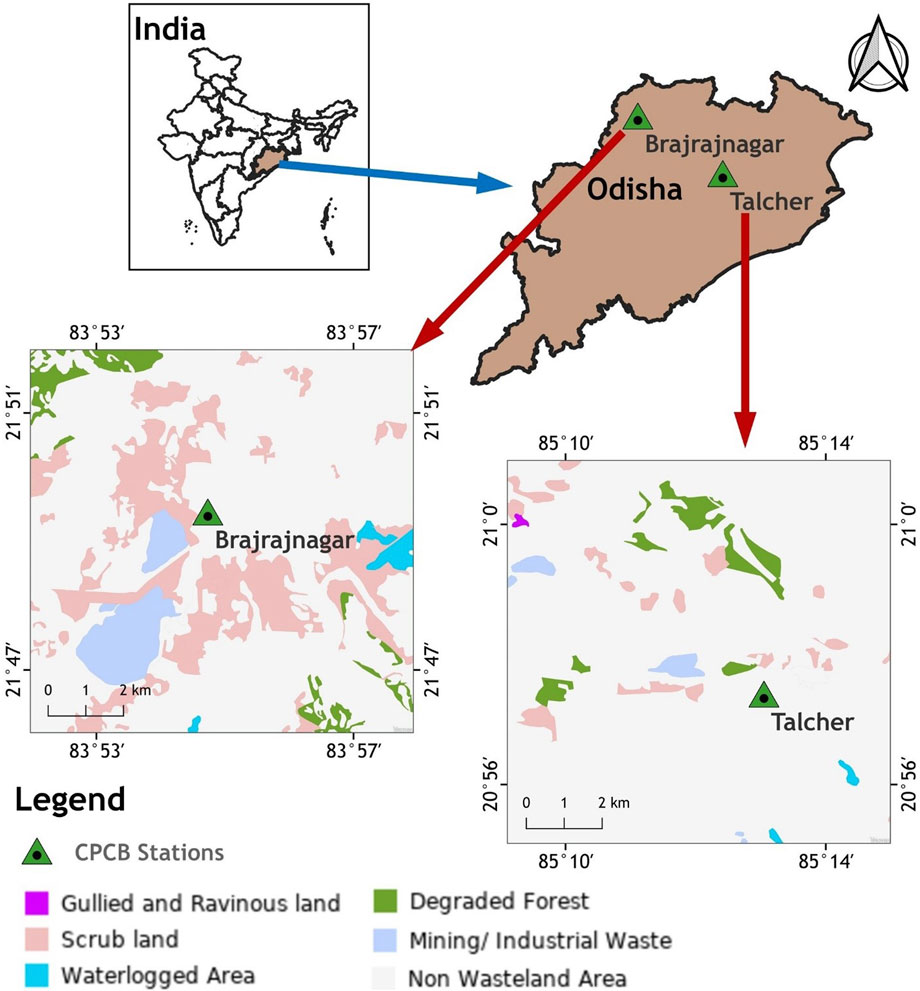
FIGURE 1. Geographical location of study area.

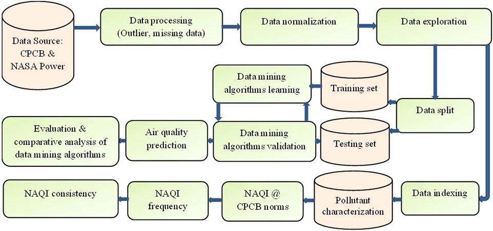
FIGURE 2. The schematic flowchart of methodology.

2.2 National air quality index (NAQI)

CPCB (2015) updated real-time NAQI in the nexus of most probable health breakpoints in six sub-indices. The cut-off levels of all six sub-indices were estimated for expected health exposure with 24 h individual pollutant concentration (8 h for CO and O₃) at monitoring stations. The methodology for computing NAQI in the proposed research is adopted from CPCB (2015), computation needs a minimum of three pollutants one must be PM_2.5 or PM₁₀. The standard permissible limits have been set by CPCB for all six criteria air pollutants and computed six NAQI levels (good to severe) and associated health impact (Table 1). The computations of sub-indices for n pollutants are evaluated by sub-indices functions.

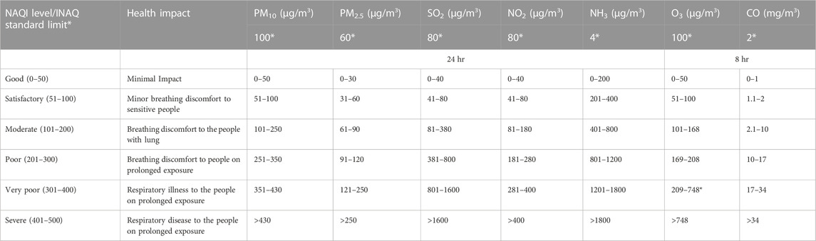
TABLE 1. NAQI level (unitless), health Impact, and health breakpoints for air pollutants.

The sub-indices computation includes addition and or multiplication; details are reported in the literature (Das et al., 2022). The computation of I_i (Sahu and Kota, 2017; Das et al., 2022) is demonstrated in Equation 3.

where, $B_{HI}$ means breakpoint concentration ≥ known concentration; $B_{L0}$ stands for breakpoint concentration ≤ known concentration; $I_{HI}$ means NAQI value equivalent to $B_{HI}$; $I_{L0}$ means NAQI value equivalent to $B_{L0}$ and $C_P$ indicates pollutant concentration. The overall NAQI can be estimated by taking the maximum sub-index of constituent pollutants, denoted as dominating pollutants (Hu et al., 2015; Sahu and Kota, 2017).

2.3 Consistency of NAQI

The consistency analysis of NAQI is performed for monitoring stations - Talcher and Brajrajnagar. NAQI level has several classes (Table 1) that range from good to severe. The consistency of the individual class is analyzed as the ratio of individual NAQI class incidence to the total number of incidences (Das et al., 2022). The proposed study evaluated the frequency and consistency of NAQI class in the Talcher and Brajrajnagar to know the persistent air quality during the study period over the study sites.

PPFL represents the Pollution Presence Frequency of individual classes; ${\mathrm{X}}_{\mathrm{i}}$ denotes the number of days when the NAQI value falls within the targeted class and n stands for the total number of days used for analysis.

2.4 Predictive modelling

For the prediction of air pollutants, RF, SVM, bagged MARS and BRNN models are used in the proposed study. The predictor variables such as PM_2.5, PM₁₀, NO₂, CO, O_3, and SO₂ were evaluated for Talcher and Brajrajnagar. To ensure that the models developed will not over fit the data, and to evaluate the performance of models, we randomly partitioned the datasets into training (2/3rd) and testing (1/3rd) sets. The training data was used to calibrate the models. In the calibration phase, the training of models was done using bootstrap strategy with 20 folds, i.e., the training dataset was bootstrapped into 20 sub-datasets and the model was trained. Once the optimized model was identified, then model was tested on testing dataset. After dividing the data sets into training and testing sets, multiple times trials were made for finding out optimal parameters. Thus, the best model was selected based on training error and testing error levels.

2.4.1 Random forest

According to Breiman (2001) and Belgium and Drăguţ (2016), RF is an effective tree-based algorithm for problems relating to classification and regression. This algorithm resists overtraining, outliers in predictors, and handling missing values because all individual trees are independent, eliminating the possibility of over fitting (Breiman and Cutler, 2004). RF algorithm uses decision trees as its foundation; it constructs each tree using a bootstrap sample of data and divides each point in the tree of randomly chosen predictors (Liaw and Wiener, 2002). Utilizing the impurity Gini index, the decision trees integrate all of the trees to make predictions (Cutler et al., 2007). A preset sample subset of the available data is used by each component tree in a RF algorithm (Archer and Kimes, 2008). Different bootstrap samples are chosen randomly for training and the remaining samples (“out-of-bag” or OOB) are used for testing. The efficiency of each algorithm is then assessed using an OOB error (Breiman, 2001). Low bias and variance, lack of over fitting, low correlation of individual trees, robust error estimates, and improved prediction accuracy are a few advantages of adopting OOB error (Wiesmeier et al., 2011; Chen et al., 2014). The primary parameters needed to construct an RF algorithm are the number of trees (n), predictive variables, and split nodes (m). For example, n = 500 (Bui et al., 2016) should be large enough to ensure the diversity of the RF algorithm. In the proposed research, n = 500 and m = 1 values are selected for all air pollutants for both sites. RF model requires less running time and generates relatively less generalization error, and as the number of trees increases, the generalization error decreases (Breiman, 2001).

2.4.2 Support vector machine

The SVM algorithm is based on supervised learning methods and showed robustness for classification and regression problems; developed and introduced by Cortes and Vapnik (1995). This algorithm is used to establish an optimal separating hyper plane with maximum margin in high-dimensional feature space. To differentiate between various air quality levels, a hyper plane is created using a kernel in the high-dimensional feature space (Vapnik et al., 1997). In this work, the most popular non-linear, Radial Basis Function (RBF) kernel is utilized which has shown robustness in some previous studies (Kumar et al., 2015; 2019). The optimal values of kernel parameters like bandwidth of kernel function (σ) and Cost (C) must be identified in prediction, σ controls the level of non-linearity introduced in the algorithm. The C value regulates the balance between minimizing training error and maximizing margin, as well as function smoothness and training duration (Rashidi et al., 2016). The SVM performance is greatly influenced by the kernel function and parameters used during the development SVM algorithm. Optimization parameters used for the prediction of air pollutants using different algorithms are given in Table 2.

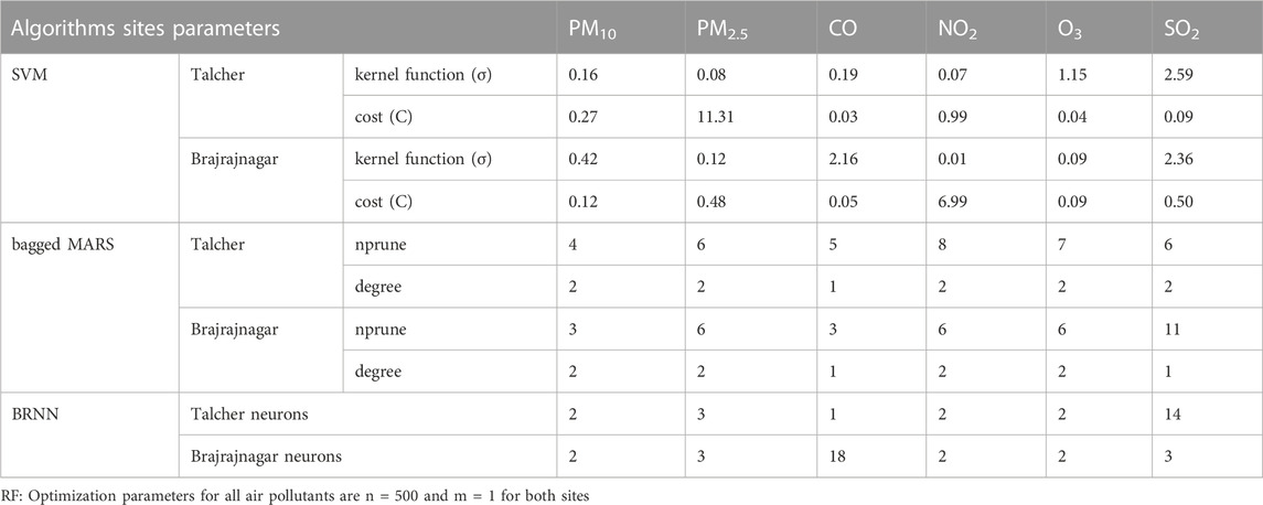
TABLE 2. Optimization parameters used for the prediction of air pollutants using different algorithms.

2.4.3 Bagged multivariate adaptive regression splines

The non-parametric, non-linear approach known as bagged MARS is used to fit the relationship between the independent and dependent variables. The target variables can be predicted by the bagged MARS algorithm using a series of coefficients and basic functions (BFs). The bagged MARS approach predicts the “BF” function using linear combinations and interactions of adaptive piecewise linear regression (Friedman, 1991). One of the benefits of the MARS algorithm, according to Cheng and Cao (2014), is its capacity to estimate the contributions of these BFs. The generated algorithm is then continuously updated with the BFs. It is widely noted that when the BFs are added, the algorithm considers the functions that cause a significant reduction in the sum of square errors. The typical form of a MARS algorithm can be expressed by the following equation (Cheng and Cao, 2014; Park et al., 2017):

where y is the dependent variables, x is the independent variables, c_o is biasing, n is the number of BF_S in the algorithm, c_i is the coefficient of the ith BF, and b_i(x) indicates the ith BF.

MARS algorithm was developed in two phases: (i) to improve algorithm performance, the forward stepwise algorithm adds BFs and looks for potential knots. However, obtaining too many BFs in this procedure can result in an over-fitted MARS algorithm. (ii) the backward stepwise algorithm, prunes redundant BFs that have the smallest contributions to the algorithm used in the forward stepwise algorithm until a suitable MARS is presented.

2.4.4 Bayesian regularized neural network

BRNN algorithm is much more robust, compared with conventional NN algorithms (Burden and Winkler, 2008). The conventional NN algorithms typically lacks satisfactory generalization ability, which leads to inaccurate air pollution prediction. Regularization is an essential procedure to improve the generalization ability of NN algorithm and to optimize regularization parameters (Ye et al., 2021). By incorporating a weight decay function into the NN’s energy function, regularization is achieved. BRNN avoids over fitting and overtraining because the network trains on useful network parameters or weights and disregards the irrelevant parameters. The following equation can be used to define the training objective function F(ω) utilized by the BRNN algorithm (Yue et al., 2011):

where S_ω is the total sum of squared network weights, S_e is the total sum of network errors, and α and β stand for the hyper parameters. Squared errors and weights are combined, and their sum is minimized until the ideal combination is found for which the network generalizes well.

The effects of noise are effectively suppressed and the NN’s capacity for generalization is increased, in the current work. The goal of training a NN is typically to provide a set of network weights and biases that minimize the error between observed air pollutants and predicted air pollutants. Theoretically intricate input-output relationships can be revealed by BRNN, making it a powerful prediction algorithm (Kayri, 2016; Okut, 2016). Even though BRNN takes up a lot of time, it can be used with small or noisy datasets. Training is continued until the optimum weights are identified (Aneja et al., 2021).

2.5 Performance investigation metrics

To make a reasonable evaluation for each prediction model, the subsequent error standards are adopted to measure the prediction accuracy, with correlation coefficient (r), root means square error (RMSE), PBias, fractional bias (FB), and fractional variance (FV) (Eqs 8–12).

where r is the correlation coefficient, and n is the number of data points to be trained or tested. $C_p$ and $C_o$ are the predicted and observed values, respectively. $\overline{C_p}$ and $\overline{C_o}$ are their respective means. ${\mathrm{\sigma }}_{{\mathrm{C}}_{\mathrm{p}}}$ and ${\mathrm{\sigma }}_{{\mathrm{C}}_{\mathrm{o}}}$ are the respective standard deviations. A closer value of r to 1 denotes a better algorithm fit, whereas a closer value to 0 indicates a worse algorithm fit. In common, good predictive algorithms are allied with smaller values of RMSE and PBias. RMSE provides a comprehensive idea of the difference between observed and predicted values. PBias is used for the identification of the details regarding over and under-predicted values (Salazar-Ruiz et al., 2008). According to the Moriasi et al. (2007) performance ratings fall into the “Satisfactory” (±30 < PBias < ±55), ‘Unsatisfactory’ (PBias > ±55), ‘Very good’ (PBias < ±15), and ‘Good’ (±15 < PBias < ±30) ranges. The mean observed values and the mean predicted values can be compared using the normalized measure FB. A normalized measure called FV enables comparisons of variance differences between predicted and observed data. A model with FV = 0 quantities can be viewed in that variance of predicted values of the model is equal to the variance of observed values.

3 Results and discussion

3.1 Criteria pollutants characterization

The study regions are populated with various types of industrial components, which are the major source of deteriorated air quality in the surroundings of Talcher and Brajrajnagar. The PM_2.5 and PM₁₀ concentration levels showed slightly decreased values throughout both lockdown periods (25th March to 31st may 2020 and 5th may to 31st may 2021). High SO₂ concentration is attribution of the industrial sources. Guttikunda and Jawahar (2018) suggested that eastern states like Odisha, West Bengal, and Jharkhand in India have high PM_2.5 pollution loads due to the expansion of coal-fired power plants. The box plots depicted the distribution of data for six air pollutants from 01 January 2019, to 01 June 2021 (Figure 3). It is observed that at Talcher around 50% of data distribution was between the 25th to 75th percentile and the remaining 40%–50% of data lies between the lower and upper whisker and up to 5% of data is displayed as an outlier, particularly in the year 2019 and 2020. At Brajrajnagar around 80% of data was distributed between 25% and 75% and up to 19% of data was distributed between upper and lower whiskers. Only 1% of data is found as an outlier. This nature of the distribution is consistent with the study period.

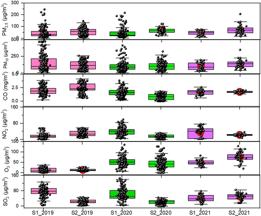
FIGURE 3. Characterization and distribution of criteria pollutants for Talcher (S1) and Brajrajnagar (S2) monitoring stations (2019–2021), eastern coastal states in India.

The inclusive concentrations of air pollutants over both monitoring stations are as follows, PM_2.5 ranges from 2.49 to 245.57 μg/m³ with mean value 57.08 μg/m³; PM₁₀ ranges from 4.83 to 348.17 μg/m³ with mean value 125.39 μg/m³; CO ranges 0.2–4.13 mg/m³ with mean value 1.57 mg/m³; SO₂ ranges 2.73–146.22 μg/m³ with mean value 48.44 μg/m³; NO₂ ranges 1.49–99.08 μg/m³ with mean value 27.35 μg/m³ and O₃ ranges 1.02–134.82 μg/m³ with mean value 44.12 μg/m³. The range of pollutants concentration is presented in Supplementary Table S1. The distribution pattern revealed that 95% of data (out of this 50% of data lies within the 1^st and third quartile) was within the lower and upper whiskers. The average concentration of PM_2.5, PM_10, and CO was higher than the NAQI standard limit (around 50% days of the study period), suggesting that the PMs are the dominant and key pollutants governing local air quality. The eastern coastal state Odisha is accounted as a hotspot in the last decades (Ghude et al., 2008; Sahu et al., 2017), residential burning of coal for household cooking is further adding up to local air pollution in the region (Tyagi et al., 2021).

3.2 Air pollutants and meteorological variables

The meteorological conditions often play important roles in local air quality through accumulation or ventilation of pollutants. Statistical analysis of air pollution data and meteorological variables reveals that at Talcher, PM_2.5 and PM₁₀ have a very good correlation (r = 0.82), and the other set of variables, PM_2.5 and temperature (r = 0.65); and PM₁₀ and temperature (r = 0.50) showed good correlation. A moderate correlation is found between RH and precipitation; temperature and WS; PM_2.5 and WS; PM₁₀ and WS, CO; NO₂ and O₃; and SO₂ and O₃. At Brajrajnagar, PM_2.5 and PM₁₀ showed a very good correlation (r = 0.94) with each other. PM_2.5 and temperature (r = 0.49); PM_2.5 and NO₂ (r = 0.58); CO and NO₂ (r = 0.67) and PM₁₀ and NO₂ (0.54) showed good correlation. A moderate correlation is found between RH and precipitation; PM_2.5 and RH, CO, precipitation; PM₁₀ and RH, precipitation, temperature; NO₂ and RH; and O₃ and CO, RH. Other air pollutants showed a poor correlation between meteorological variables. The detailed descriptive statistics between air pollutants and meteorological variables for Talcher and Brajrajnagar are presented in Figure 4; Supplementary Table S2.

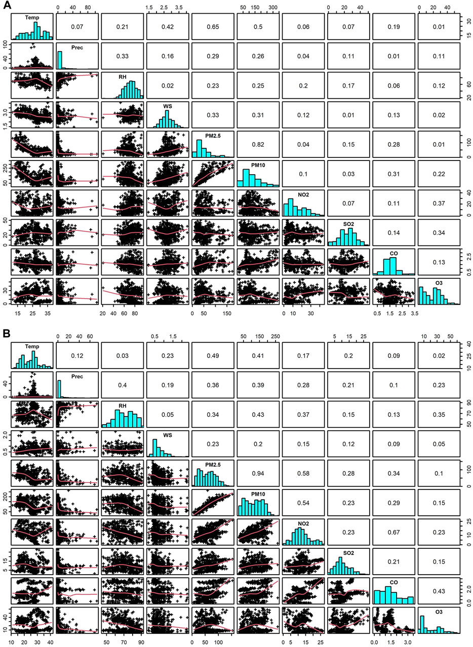
FIGURE 4. Correlation matrix between air pollutants and meteorological variables for (A) Talcher and (B) Brajrajnagar sites, eastern coastal state in India.

3.3 NAQI and sub-indices

The NAQI is the weighted addition of sub-indices of pollutants. The sub-indices of PM_2.5 and PM₁₀ are deciding components of NAQI in 90% of the cases (Sahu and Kota, 2017). The sub-AQI of PM_2.5 and PM₁₀ distribution showed that >50% of days PM_2.5 concentration was higher than the NAQI standard limit (100 μg/m³ and 60 μg/m³, respectively). The CO concentration NAQI limit is 2 mg/m³. It is observed that around 40% of days in the year 2019 sub-indices of CO exceeded the NAQI limit but comparatively more days were found within the CO-indices NAQI standard limit in years 2020 and 2021. The sub-indices of NO₂ distribution are found within NAQI standard limit (80 μg/m³) for both monitoring stations. However, absolute concentration has been found to be increased in the successive year from 2019 to 2021 at Talcher and the vice versa pattern is observed at Brajrajnagar. The comparative increase in the absolute magnitude of O₃ sub-indices is observed for both the monitoring stations and noticed that only for a few days in the years 2020 and 2021 the O₃ sub-indices exceeded the NAQI standard limit. The absolute sub-indices of SO₂ at Talcher dropped in progressive years as compared to the year 2019 and the number of days that exceeded the NAQI standard limit also decreased in successive years from 2019 to 2021. The sub-indices distribution over Brajrajnagar is similar to Talcher but for the year 2021, many days exceeded the SO₂ NAQI standard limit (80 μg/m³).

It is observed that Talcher station had satisfactory and moderate class NAQI, on most of the days in the year 2019. Similarly, in the year 2020 NAQI distribution ranges from satisfactory to very poor class, with maximum days the air quality lies in moderate class. In the year 2021, NAQI is observed in two classes, satisfactory and moderate. The slight improving air quality in the years 2020 and 2021 was due to the enforced restriction on the roadway and commercial activity as a precautionary step to control COVID-19 (Baweja et al., 2022). At Talcher, good NAQI days are zero whereas at Brajrajnagar station NAQI distribution depicted a wide range of NAQI classes, mostly moderate to poor days NAQI, and for a few days, air quality lies between satisfactory to the very poor class. In the year 2020, for a few days, air quality was good, poor, and very poor whereas, for a significant number of days, NAQI was within the moderate and satisfactory class. Similarly, in the year 2021 at Brajrajnagar, NAQI distribution was found in the class of satisfactory to very poor with maximum days with moderate NAQI class as shown by Sharma et al. (2020) and Baweja et al. (2022). The pollutant-wise sub-indices and NAQI for air quality monitoring stations for Talcher and Brajrajnagar, a coalmine complex area, for three consecutive years 2019–2021, are shown in Figure 5.

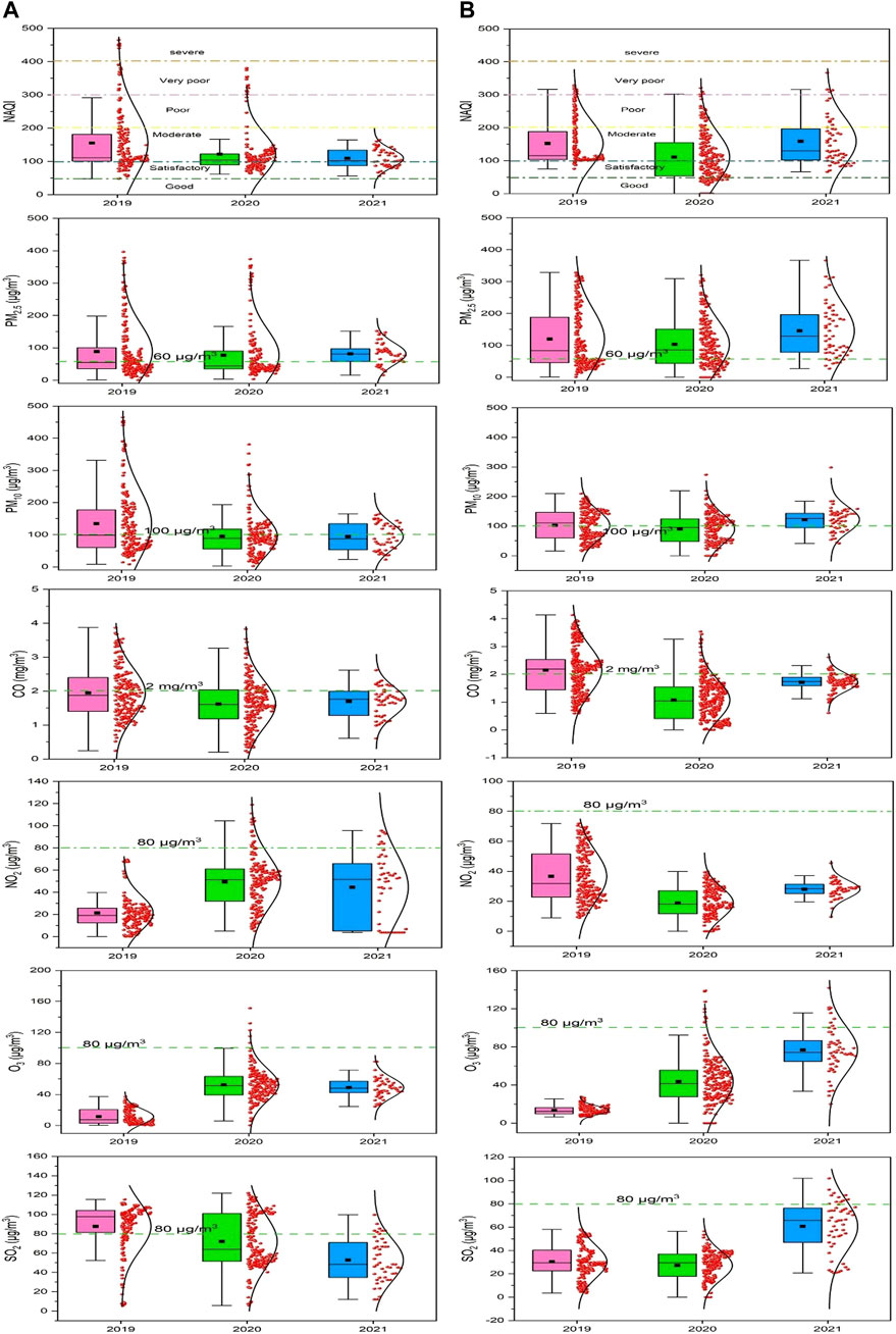
FIGURE 5. NAQI and criteria pollutants sub-indices for Talcher (A) and Brajrajnagar (B) monitoring stations, eastern coastal states in India.

3.4 NAQI frequency and consistency

The comparative aspects of 3 years (2019–2021) of NAQI frequency (Supplementary Table S3) and consistency (Supplementary Table S4) distribution of different levels are portrayed in bubble plots (Figure 6) for both monitoring sites. It is observed that NAQI ranges from 101–200 (moderate level) and has a maximum frequency of occurrence of 26–108 and 27–158 days during the year 2019–2021 at Talcher and Brajrajnagar, respectively. NAQI level of 51–100 (satisfactory class) has a frequency of occurrence of 20–67 and 13–60 days during 2019–2021at Talcher and Brajrajnagar, respectively. The consistency of satisfactory level NAQI ranges from 22% to 3% to 4%–28% at Talcher and Brajrajnagar, respectively. The consistency of satisfaction increased from 22% in 2019 to 43% in 2021 at Talcher and 4% in 2019 to 28% at Brajrajnagar in the year 2020.

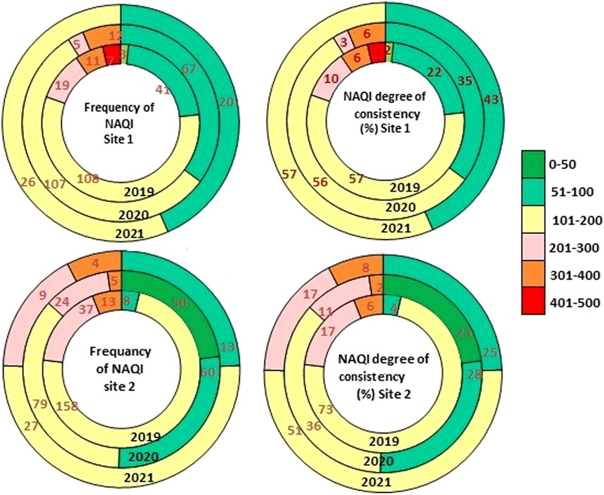
FIGURE 6. Bubble plots for frequency of occurrence and consistency (in percentage) of NAQI class for monitoring stations Talcher and Brajrajnagar, eastern coastal states in India.

The poor level NAQI (201–300) frequency of occurrence ranges from 5 to 19 and 9–37 days at Talcher and Brajrajnagar, respectively. The consistency of NAQI 201–300 level ranges from 3% to 10% and 11%–17% at Talcher and Brajrajnagar, respectively. The very poor NAQI class (301–400) frequency ranges from 11 to 12 days at Talcher and 4–13 days at Brajrajnagar and consistency ranges from 2% to 8% at both sites. It is noticeable that in the year 2019, the consistency and frequency of occurrence of NAQI levels 101–200, and 201–300 were higher as compared to the years 2020 and 2021. However, at a satisfactory level air quality frequency of occurrence and consistency was lower in the year 2019 and higher in the year 2020 and 2021 due to shut down of anthropogenic activities. The difference in moderate and poor level NAQI in the year 2020–2021 as compared to 2019 is due to imposed restrictions on roadway transport and commercial activities due to the pandemic event. Economic activities in the neighboring areas had a great impact on air quality, and during the fraction of this study period (2020–2021), the commercial activities were forced to shut down to control COVID-19 dispersion (Das et al., 2022). However, not much significant difference in air quality was obtained since the thermal power plants and coal mines (associated activities mining, coal transport, coal dumping, etc.) were operational during the study period. Therefore, a minor difference in NAQI in the year 2020–2021 is found as compared to the year 2019 NAQI. Similar results were reported by Shairsingh et al. (2018) and Mihankhah et al. (2020). The results indicate that industrial regions are more prone to high PMs concentrations and higher NAQI levels as compared to commercial and residential sectors.

3.5 Prediction using RF, SVM, bagged MARS, and BRNN algorithms

Monitoring and predicting air quality have become basically significant in real time, particularly in emerging nations like India (Kumar and Pande, 2022). The machine leaning based forecast models have been ended up being more reliable. The precise and robust prospects of large data can be managed proficiently with ML algorithms (Gladkova and Saychenko, 2022). This recent article proposed comprehensive robust models to predict AQI accurately, at Talcher and Brajrajnagar. ML models like RF, SVM, bagged MARS, and BRNN were employed here to predict the AQI, because these models have shown their robustness to enhance AQI worldwide. The prediction of the AQI not only requires the selection of a good choice of prediction model, it requires attention to multiple factors, including the missing observations in raw training data, the high inconsistency in data, proper selection of predictors, meteorology and high temporal correlations between the concentrations of pollutants and its accurate parameters tuning. This paper proposed ML models considering all of these factors. r, RMSE, Pbias, FB and FV were the performance metrices considered to evaluate the performance of the model. The prediction of pollutant’s level with the selected features was adequate for almost all the pollutants to improve prediction accuracy of AQI. Further analysis and testing may be taken using additional features for predicting CO levels, as it would enhance overall AQI prediction. Since its predictions were the least accurate for both the sits.

The scatter plots between observed and predicted values of training and testing data are depicting strong correlation in case of PM_2.5 (Figure 7) and PM₁₀ (Figure 8) for all models at Talcher and Brajrajnagar sites. The mostly scattered points are lying over the best fit line at the centre of the plots. The low and comparable RMSE between observed and predicted values of PM_2.5 are indicating about slightly better prediction of PM_2.5 by RF (Training RMSE = 12.40 μg/m³; Testing RMSE = 17.90 μg/m³), SVM (Training RMSE = 16.76 μg/m³; Testing RMSE = 17.54 μg/m³), bagged MARS (Training RMSE = 16.86 μg/m³; Testing RMSE = 17.64 μg/m³), and BRNN (Training RMSE = 16.79 μg/m³; Testing RMSE = 17.53 μg/m³) models at Talcher site in comparison to Brajrajnagar site. However, PM₁₀ (RMSE = 25.80–43.41 μg/m³, NO₂ (RMSE = 3.00–4.95 ppb) and SO₂ (RMSE = 2.78–5.46 ppb) at Brajrajnagar are better than PM₁₀ (RMSE = 35.40–55.33 μg/m³), NO₂ (RMSE = 4.99–9.11 ppb), and SO₂ (RMSE = 4.91–9.47 ppb) between observed and predicted values of training and testing data at Talcher using RF, SVM, bagged MARS and BRNN models, respectively. Low PM₁₀ RMSE between observed and predicted values of training (RMSE = 25.80 μg/m³) and testing (RMSE = 38.72 μg/m³) data using RF model are slightly better at Brajrajnagar in comparison to SVM, bagged MARS and BRNN models of both sites. Whereas, moderate correlation between observed and predicted values of training and testing data for all the models were identified in case of NO₂ (at both site) (Figure 9) and O₃ (at Brajrajnagar site) (Figure 10). RF model training data showed strong correlation between observed and predicted values in case of CO, O₃ and SO₂ at both sites. Though, SVM, bagged MARS and BRNN models illustrating weaker correlation between observed and predicted values of CO and SO₂ at both sites (Supplementary Figures S1, S2). The predicted values of PM_2.5, PM₁₀, NO₂, SO₂, CO, and O₃ using training datasets are compared with measured air pollutants. The trained algorithms are verified using the testing dataset for the prediction of air pollutants. The predicted air pollutant values using testing datasets are compared with the in-situ measured air pollutants. Importantly, all algorithms showed good performance except CO and O₃, which highlighted overall capabilities in modeling air pollutants. Low-magnitude values of P bias indicate accurate model simulation, with 0.0 being the ideal value. The negative values indicate model underestimation bias, whereas positive values indicate overestimation bias. SVM algorithm was given high under estimated Pbias (−11.78) for NO₂ prediction and overestimated Pbias (5.38) for SO₂ prediction at Talcher site. Though, at Brajrajnagar site high under estimated Pbias (−9.21) was for SO₂ using SVM algorithm and overestimated Pbias (4.38) was for CO using RF algorithm. Statistical analysis concluded that SVM algorithm results are moderate in comparison to RF algorithm in the time series data investigation. The predicted accuracy of the results of PM_2.5, PM_10, NO_2, and O₃ using the RF model in this study for both sites are similar in compare to predicted PM_2.5, PM_10, NO_2, and O₃ using RF model by Gariazzo et al. (2020) in Italy. Chen et al. (2019) predicted similar results in China for PM_2.5 using the RF model. The performance of different algorithms is evaluated in terms of r, RMSE, P bias, FB, and FV are presented in detail in Table 3.

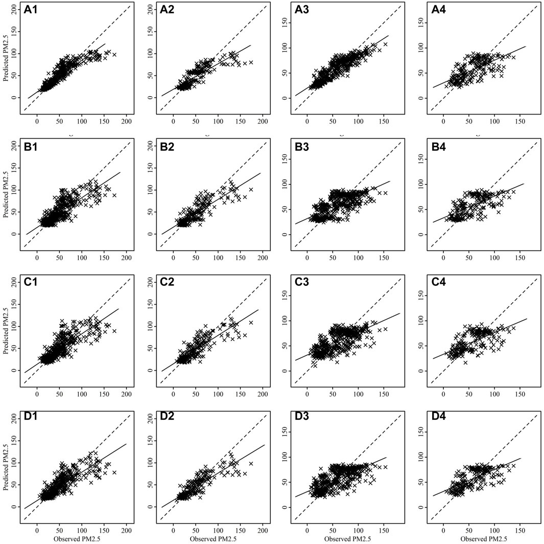
FIGURE 7. Scatter plots between observed and predicted values of PM_2.5 for training [(A1–D1) for Talcher and (A3–D3) for Brajrajnagar] and testing [(A2–D2) for Talcher and (A4–D4) for Brajrajnagar]. Where plots are for RF (A1-A4), bagged MARS (B1–B4), BRNN (C1–C4) and SVM (D1-D4) algorithms.

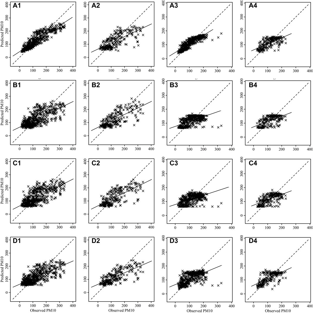
FIGURE 8. Scatter plots between observed and predicted values of PM₁₀ for training [(A1–D1) for Talcher and (A3–D3) for Brajrajnagar] and testing [(A2–D2) for Talcher and (A4–D4) for Brajrajnagar]. Where plots are for RF (A1–A4), bagged MARS (B1–B4), BRNN (C1–C4) and SVM (D1–D4) algorithms.

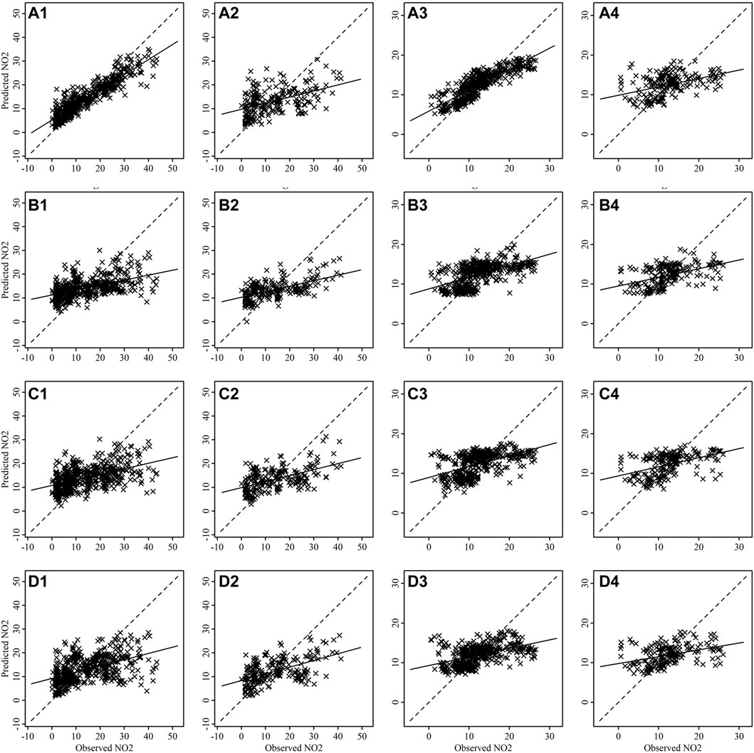
FIGURE 9. Scatter plots between observed and predicted values of NO₂ for training [(A1-D1) for Talcher and (A3–D3) for Brajrajnagar] and testing [(A2-D2) for Talcher and (A4–D4) for Brajrajnagar]. Where plots are for RF (A1–A4), bagged MARS (B1–B4), BRNN (C1–C4) and SVM (D1–D4) algorithms.

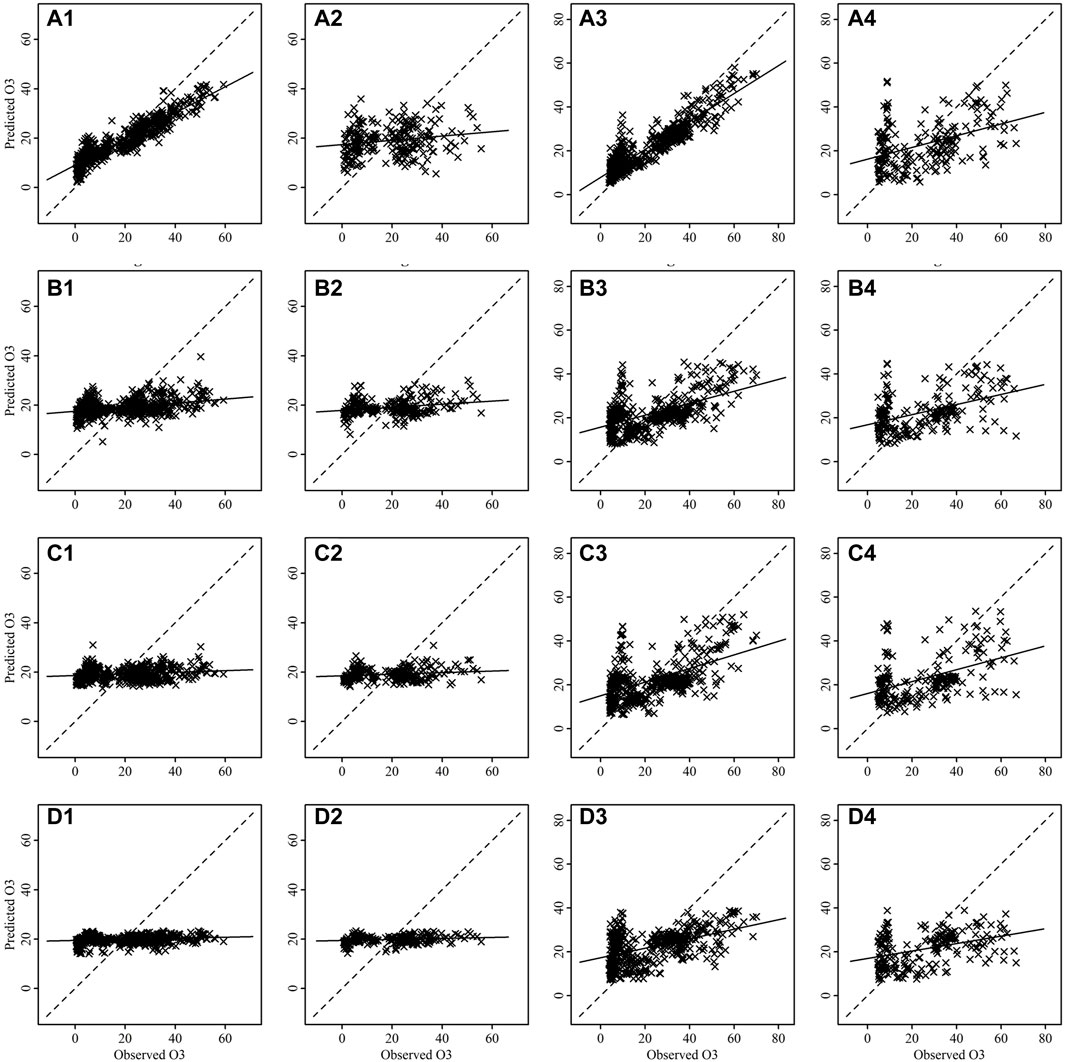
FIGURE 10. Scatter plots between observed and predicted values of O₃ for training [(A1–D1) for Talcher and (A3–D3) for Brajrajnagar] and testing [(A2–D2) for Talcher and (A4–D4) for Brajrajnagar]. Where plots are for RF (A1–A4), bagged MARS (B1–B4), BRNN (C1–C4) and SVM (D1–D4) algorithms.

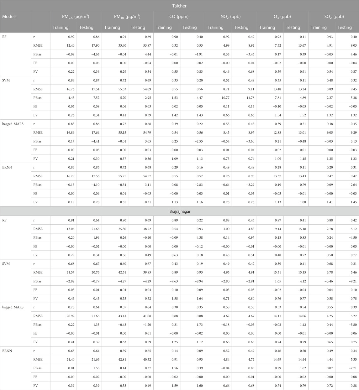
TABLE 3. Comparative statistical analysis for the prediction of air pollutants using different optimized algorithms.

3.6 Performance evaluation of air pollutants using different algorithms by Taylor diagram

Taylor diagram is used to display the graphical representation of the model performance in terms of r, centered Root-Mean Square Difference (cRMSD), and standard deviation (SD) using training and testing datasets, respectively. The radial distance from the origin is represented by the SD values. The cRMSD is the distance between the modeled data and the observed data (measured in the same units as the SD) (Taylor, 2001). The performance of RF, SVM (radial), bagged MARS, and BRNN algorithms to predict PM_2.5, PM₁₀, CO, NO₂, O_3, and SO₂ are compared using the Taylor diagram. Using observed data, the Taylor plot’s circle mark along the X-axis is designated as the reference point. Overestimation will arise if the SD of the predicted values is larger than the SD of the observed values, and vice versa (Gupta et al., 2017; Chaudhary et al., 2022). Taylor plot also shows a strong correlation between the observed and predicted values of air pollutants during the training and testing of all algorithms. RF model provided higher efficiency in comparison to SVM, bagged MARS, and BRNN in the training of all air pollutants at both monitoring sites. Though for testing of data, the RF model has provided results analogous to SVM, bagged MARS, and BRNN models at Talcher and Brajrajnagar sites. All algorithms have shown higher efficiency for PM_2.5 and PM₁₀ except being for CO and O₃ at Talcher and CO at Brajrajnagar. The results are found moderate in the prediction of NO₂ and SO₂ using all models at both sites. The evaluation of different air pollutants using RF, SVM (radial), bagged MARS and BRNN algorithms by Taylor diagram are shown at Talcher (Figure 11) and Brajrajnagar (Figure 12). The suggested research’s findings are currently viewed as a useful practical tool that may be increasingly helpful for decision-makers and environmental management and to gain new insights into air quality modeling.

FIGURE 11. Evaluation of different air pollutants using bagged MARS, RF, SVM (radial), and BRNN algorithms by Taylor diagram at Talcher.

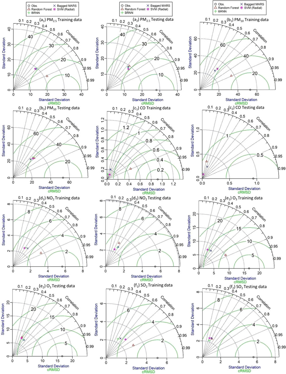
FIGURE 12. Evaluation of different air pollutants using bagged MARS, RF, SVM (radial), and BRNN algorithms by Taylor diagram at Brajrajnagar.

4 Conclusion

As the source strength of air pollutants differ spatio-temporal, it is of extreme priority to understand distribution of harmful air pollutants to lay out optimum benefit control strategies in urban-rural stretch and coal-mine complex belt of an eastern coastal state, Odisha. The PM_2.5 and PM₁₀ concentration levels slightly decreased during 2020 at Brajrajnagar, and during 2021 at both sites. High SO₂ concentration is primarily attributed to industrial sector, which favors rise of O₃ levels. The concentration of PM_2.5, PM_10, and CO is higher than the NAQI standard limit (around 50% days of the study period), indicating the issue of air pollution and deteriorated local air quality in and around the mining area. Among pollutant sub-indices around 90% of the cases PM_2.5 and PM₁₀ are deciding components of NAQI. Around 26–158 days with the consistency of 36%–73% moderate level air quality prevail over the study period of 2019–2021. Whereas, satisfactory level air quality prevails up to 4–43 days with a consistency of 13%–67%. Remarkably, it is observed that a satisfactory level of air quality consistency increased from 22% to 43% at Talcher and 4%–28% at Brajrajnagar during 2020 and 2021 as compared to 2019. This small improvement in air quality during 2020–2021 timeframe was due to shut-off of anthropogenic activities in the state. RF, SVM, Bagged MARS and BRNN showed higher efficiency for the prediction of PM_2.5, PM₁₀, SO_2, and NO₂ except CO and O₃ at Talcher and CO at Brajrajnagar. Though the RF model showed higher r values between observed and predicted values for training data in comparison to SVM, Bagged MARS and BRNN models. Statistical analysis and Taylor plots demonstrated that the proposed algorithms showed promising accuracy for predicting air quality. The experimental findings demonstrate that the suggested algorithms can enhance the generalization ability of data mining, and outperform several established prediction models in terms of prediction accuracy.

Data availability statement

The raw data supporting the conclusions of this article will be made available by the authors, without undue reservation.

Author contributions

AC: methodology, formal analysis, data curation, writing–original draft, review and editing; PK: methodology, formal analysis, data curation, writing–original draft, review, and editing; CP: review and editing; SS: review and editing; SC: review and editing; PJ: review and editing; DeP: review and editing; DiP: review and editing; AM: review and editing.

Funding

RUSA (Rashtriya Uchchatar Shiksha Abhiyan), order no. RUSA-1041-2016(PDF-XVIII) 25986/2020 for providing fellowship; Dr. DSK-Post Doctoral Fellowship by University Grant Commission (UGC), sanction No.F.4-2/2006 (BSR)/ES/18-19/0041.

Acknowledgments

The AC would like to acknowledge RUSA, a central government scheme, order no. RUSA-1041-2016(PDF-XVIII) 25986/2020, regarding the financial support under RUSA 2.0 project. We are also grateful to CPCB, Govt. of India, for providing free accessible air pollutants data and NASA for meteorological variables. PK is thankful to UGC, for Dr. DSK-PDF award by UGC sanction No.F.4-2/2006 (BSR)/ES/18-19/0041.

Conflict of interest

The authors declare that the research was conducted in the absence of any commercial or financial relationships that could be construed as a potential conflict of interest.

Publisher’s note

All claims expressed in this article are solely those of the authors and do not necessarily represent those of their affiliated organizations, or those of the publisher, the editors and the reviewers. Any product that may be evaluated in this article, or claim that may be made by its manufacturer, is not guaranteed or endorsed by the publisher.

Supplementary material

The Supplementary Material for this article can be found online at: https://www.frontiersin.org/articles/10.3389/fenvs.2023.1132159/full#supplementary-material

References

Abirami, G., Girija, R., Das, A., and Sreenivasan, N. (2022). “Predicting air quality index with machine learning models,” in Machine learning and deep learning in efficacy improvement of healthcare systems (CRC Press), 353–371.
Aneja, S., Sharma, A., Gupta, R., and Yoo, D. Y. (2021). Bayesian regularized artificial neural network model to predict strength characteristics of fly-ash and bottom-ash-based geopolymer concrete. Materials 14 (7), 1729. doi:10.3390/ma14071729
Archer, K. J., and Kimes, R. V. (2008). Empirical characterization of random forest variable importance measures. Comput. Stat. Data Anal. 52 (4), 2249–2260. doi:10.1016/j.csda.2007.08.015
Baldasano, J. M., Valera, E., and Jiménez, P. (2003). Air quality data from large cities. Sci. Total Environ. 307 (1-3), 141–165. doi:10.1016/s0048-9697(02)00537-5
Baweja, P., Chopra, H., Gandhi, P. B., Gupta, S., Poddar, N., Suman, S., et al. (2022). Tale of air quality index (AQI) in India: pre-and during the COVID-19 pandemic.
Belgiu, M., and Drăguţ, and L. (2016). Random forest in remote sensing: a review of applications and future directions. ISPRS J. Photogramm. Remote Sens. 114, 24–31.
Breiman, L., and Cutler, A. (2004). Random forests. (URL) http://www.stat.berkeley.edu/users/Breiman/RandomForests/ccpapers.html.
Bui, D. T., Pradhan, B., Nampak, H., Quang Bui, T., Tran, Q.-A., and Nguyen, Q. P. (2016). Hybrid artificial intelligence approach based on neural fuzzy inference model and metaheuristic optimization for flood susceptibility modelling in a high-frequency tropical cyclone area using GIS. J. Hydrol. 540, 317–330.
Burden, F., and Winkler, D. (2008). “Bayesian regularization of neural networks,” in Methods in molecular biolog (Totowa, NJ, USA: Humana Press), 23–42.
Chaudhary, S. K., Srivastava, P. K., Gupta, D. K., Kumar, P., Prasad, R., Pandey, D. K., et al. (2022). Machine learning algorithms for soil moisture estimation using Sentinel-1: model development and implementation. Adv. Space Res. 69 (4), 1799–1812. doi:10.1016/j.asr.2021.08.022
Chen, J., Yin, J., Zang, L., Zhang, T., and Zhao, M. (2019). Stacking machine learning model for estimating hourly PM2. 5 in China based on Himawari 8 aerosol optical depth data. Sci. Total Environ. 697, 134021. doi:10.1016/j.scitotenv.2019.134021
Chen, K. Y. (2011). Combining linear and nonlinear model in forecasting tourism demand. Expert Syst. Appl. 38, 10368–10376. doi:10.1016/j.eswa.2011.02.049
Chen, W., Li, X., Wang, Y., Chen, G., and Liu, S. (2014). Forested landslide detection using LiDAR data and the random forest algorithm: a case study of the three gorges, China. Remote Sens. Environ. 152, 291–301.
Cheng, M. Y., and Cao, M. T. (2014). Accurately predicting building energy performance using evolutionary multivariate adaptive regression splines. Appl. Soft Comput. 22, 178–188. doi:10.1016/j.asoc.2014.05.015
Choudhary, A., Kumar, P., Gaur, M., Prabhu, V., Shukla, A., and Gokhale, S. (2020). Real-world driving dynamics characterization and identification of emission rate magnifying factors for an auto-rickshaw. Nat. Environ. Poll. Technol. 19 (1), 93–101.
Choudhary, A., Kumar, P., Sahu, S. K., and Pradhan, C. (2022a). Real-time roadway pollution in Indian cities: a comparative assessment with modelled emission. Res. J. Chem. Environ. 26, 97–106. doi:10.25303/2605rjce97106
Choudhary, A., Kumar, P., Sahu, S. K., Pradhan, C., Singh, S. K., Gašparović, M., et al. (2022b). Time series simulation and forecasting of air quality using in-situ and satellite-based observations over an urban region. Nat. Environ. Poll. Technol. 21, 1137–1148. doi:10.46488/nept.2022.v21i03.018
Cohen, A. J., Brauer, M., Burnett, R., Anderson, H. R., Frostad, J., Estep, K., et al. (2017). Estimates and 25-year trends of the global burden of disease attributable to ambient air pollution: an analysis of data from the Global Burden of Diseases Study 2015. Lancet 389 (10082), 1907–1918. doi:10.1016/s0140-6736(17)30505-6
Cortes, C., and Vapnik, V. (1995). Support-vector networks. Mach. Learn. 20, 273–297. doi:10.1007/bf00994018
CPCB (2009). National ambient air quality standards. New Delhi, India: Central Pollution Control Board.
CPCB (2015). Central Pollution Control Board National air quality index. Control of urban pollution series, CUPS/82/2014-15. Ministry of Environment Forest and Climate Change, Govt. of India http://164.100.107.13/FINAL-EPORT_AQI_.pdf.
Cutler, D. R., Edwards, T. C., Beard, K. H., Cutler, A., Hess, K. T., Gibson, J., et al. (2007). Random forests for classification in ecology. J. Ecol. 88 (11), 2783–2792. doi:10.1890/07-0539.1
Das, P., Mandal, I., Pal, S., Mahato, S., Talukdar, S., and Debanshi, S. (2022). Comparing air quality during nationwide and regional lockdown in Mumbai Metropolitan City of India. Geocarto Int. 37, 10366–10391. doi:10.1080/10106049.2022.2034987
Friedman, J. H. (1991). Multivariate adaptive regression splines. Ann. Stat. 19, 1–141. doi:10.1214/aos/1176347963
Gal, Y., and Ghahramani, Z. (2016). A theoretically grounded application of dropout in recurrent neural networks. Proc. 30th NeurlPS, 1027–1035.
Gariazzo, C., Carlino, G., Silibello, C., Renzi, M., Finardi, S., Pepe, N., et al. (2020). A multi-city air pollution population exposure study: combined use of chemical-transport and random-Forest models with dynamic population data. Sci. Total Environ. 724, 138102. doi:10.1016/j.scitotenv.2020.138102
Ghude, S. D., Fadnavis, S., Beig, G., Polade, S. D., and Van Der A, R. J. (2008). Detection of surface emission hot spots, trends, and seasonal cycle from satellite-retrieved NO2 over India. J. Geophys. Res. Atmos. 113 (D20). doi:10.1029/2007jd009615
Gladkova, E., and Saychenko, L. (2022). Applying machine learning techniques in air quality prediction. Transp. Res. Procedia 63, 1999–2006. doi:10.1016/j.trpro.2022.06.222
Gocheva-Ilieva, S., Ivanov, A., and Stoimenova-Minova, M. (2022). Prediction of daily mean PM10 concentrations using random forest, CART Ensemble and Bagging Stacked by MARS. Sustainability 14 (2), 798. doi:10.3390/su14020798
Gupta, D. K., Prasad, R., Kumar, P., and Vishwakarma, A. K. (2017). Soil moisture retrieval using ground-based bistatic scatterometer data at X-band. Adv. Space Res. 59 (4), 996–1007. doi:10.1016/j.asr.2016.11.032
Gupta, N. S., Mohta, Y., Heda, K., Armaan, R., Valarmathi, B., and Arulkumaran, G. (2023). Prediction of air quality index using machine learning techniques: a comparative analysis. J. Environ. Public Health 2023, 1–26. doi:10.1155/2023/4916267
Guttikunda, S. K., and Jawahar, P. (2018). Evaluation of particulate pollution and health impacts from planned expansion of coal-fired thermal power plants in India using WRF-CAMx modeling system. Aerosol Air Qual. Res. 18 (12), 3187–3202. doi:10.4209/aaqr.2018.04.0134
Hu, J., Ying, Q., Wang, Y., and Zhang, H. (2015). Characterizing multi-pollutant air pollution in China: comparison of three air quality indices. Environ. Int. 84, 17–25. doi:10.1016/j.envint.2015.06.014
Kalbande, R., Kumar, B., Maji, S., Yadav, R., Atey, K., Rathore, D. S., et al. (2023). Machine learning based quantification of VOC contribution in surface ozone prediction. Chemosphere 326, 138474. doi:10.1016/j.chemosphere.2023.138474
Kayri, M. (2016). Predictive abilities of bayesian regularization and levenberg–marquardt algorithms in artificial neural networks: a comparative empirical study on social data. Math. Comput. Appl. 21 (2), 20. doi:10.3390/mca21020020
Kumar, K., and Pande, B. P. (2022). Air pollution prediction with machine learning: a case study of Indian cities. Int. J. Environ. Sci. Tech. 20, 5333–5348. doi:10.1007/s13762-022-04241-5
Kumar, P., Gupta, D. K., Mishra, V. N., and Prasad, R. (2015). Comparison of support vector machine, artificial neural network, and spectral angle mapper algorithms for crop classification using LISS IV data. Int. J. Remote Sens. 36 (6), 1604–1617. doi:10.1080/2150704x.2015.1019015
Kumar, P., Kapur, S., Choudhary, A., and Singh, A. K. (2022). Spatiotemporal variability of optical properties of aerosols over the Indo-Gangetic Plain during 2011–2015. Ind. J. Phy. 96 (2), 329–341. doi:10.1007/s12648-020-01987-x
Kumar, P., Prasad, R., Choudhary, A., Gupta, D. K., Mishra, V. N., Vishwakarma, A. K., et al. (2019). Comprehensive evaluation of soil moisture retrieval models under different crop cover types using C-band synthetic aperture radar data. Geocarto Int. 34 (9), 1022–1041. doi:10.1080/10106049.2018.1464601
Kumar, P., Pratap, V., Kumar, A., Choudhary, A., Prasad, R., Shukla, A., et al. (2020). Assessment of atmospheric aerosols over Varanasi: physical, optical and chemical properties and meteorological implications. J. Atmos. Solar-Terr. Phy. 209, 105424. doi:10.1016/j.jastp.2020.105424
Laña, I., Del Ser, J., Pedró, A., Vélez, M., and Casanova-Mateo, C. (2016). The role of local urban traffic and meteorological conditions in air pollution: a data-based case study in Madrid, Spain. Atmos. Environ. 145, 424–438. doi:10.1016/j.atmosenv.2016.09.052
Larkin, A., Anenberg, S., Goldberg, D. L., Mohegh, A., Brauer, M., and Hystad, P. (2023). A global spatial-temporal land use regression model for nitrogen dioxide air pollution. Front. Environ. Sci. 11, 1125979.
Lewis, P. G. T., Chiu, W. A., Nasser, E., Proville, J., Barone, A., Danforth, C., et al. (2023). Characterizing vulnerabilities to climate change across the United States. Environ. Int. 172, 107772. doi:10.1016/j.envint.2023.107772
Liu, H., Li, Q., Yu, D., and Gu, Y. (2019). Air quality index and air pollutant concentration prediction based on machine learning algorithms. Appl. Sci. 9 (19), 4069. doi:10.3390/app9194069
Mihankhah, T., Saeedi, M., and Karbassi, A. (2020). A comparative study of elemental pollution and health risk assessment in urban dust of different land-uses in Tehran’s urban area. Chemosphere 241, 124984. doi:10.1016/j.chemosphere.2019.124984
Moriasi, D. N., Arnold, J. G., Van Liew, M. W., Binger, R. L., Harmel, R. D., and Veith, T. L. (2007). Model evaluation guidelines for systematic quantification of accuracy in watershedsimulations. Trans. ASABE 50, 885–900. doi:10.13031/2013.23153
Oduro, S. D., Metia, S., Duc, H., Hong, G., and Ha, Q. P. (2015). Multivariate adaptive regression splines models for vehicular emission prediction. Vis. Eng. 3 (1), 13–12. doi:10.1186/s40327-015-0024-4
Ojha, N., Girach, I., Sharma, K., Sharma, A., Singh, N., and Gunthe, S. S. (2021). Exploring the potential of machine learning for simulations of urban ozone variability. Sci. Rep. 11 (1), 22513. doi:10.1038/s41598-021-01824-z
Okut, H. (2016). “Bayesian regularized neural networks for small n big p data,” Artificial Neural Networks-Models and Applications. London, UK: InTech.
Ortiz-García, E. G., Salcedo-Sanz, S., Pérez-Bellido, M., Portilla-Figueras, J. A., and Prieto, L. (2010). Prediction of hourly O3 concentrations using support vector regression algorithms. Atmos. Environ. 44, 4481–4488. doi:10.1016/j.atmosenv.2010.07.024
Ott, W. R. (1978). Envriron indices: theo and prac. Ann Arbor, MI. Ott: Ann Arbor Science Publishers, Inc.
Pai, P. F., Lin, K. P., Lin, C. S., and Chang, P. T. (2010). Time series forecasting by a seasonal support vector regression model. Expert Syst. Appl. 37 (6), 4261–4265. doi:10.1016/j.eswa.2009.11.076
Park, S., Hamm, S. Y., Jeon, H. T., and Kim, J. (2017). Evaluation of logistic regression and multivariate adaptive regression spline models for groundwater potential mapping using R and GIS. Sustainability 9 (7), 1157. doi:10.3390/su9071157
Piqueras, P., and Vizenor, A. (2016). The rapidly growing death toll attributed to air pollution: a global responsibility. Policy Brief GSDR, 1–4.
Prakash, D., Payra, S., Verma, S., and Soni, M. (2013). Aerosol particle behavior during Dust Storm and Diwali over an urban location in north western India. Nat. hazards 69 (3), 1767–1779. doi:10.1007/s11069-013-0780-1
Pratap, V., Kumar, A., Tiwari, S., Kumar, P., Tripathi, A. K., and Singh, A. K. (2020). Chemical characteristics of particulate matters and their emission sources over Varanasi during winter season. J. Atmos. Chem. 77 (3), 83–99. doi:10.1007/s10874-020-09405-6
Rashidi, S., Vafakhah, M., Lafdani, E. K., and Javadi, M. R. (2016). Evaluating the support vector machine for suspended sediment load forecasting based on gamma test. Arab. J. Geosci. 9, 583. doi:10.1007/s12517-016-2601-9
Sahu, S. K., and Kota, S. H. (2017). Significance of PM2. 5 air quality at the Indian capital. Aerosol Air Qual. Res. 17 (2), 588–597.
Sahu, S. K., Ohara, T., and Beig, G. (2017). The role of coal technology in redefining India’sclimate change agents and other pollutants. Environ. Res. Lett. 12 (10), 105006. doi:10.1088/1748-9326/aa814a
Salazar-Ruiz, E., Ordieres, J. B., Vergara, E. P., and Capuz-Rizo, S. F. (2008). Development and comparative analysis of tropospheric ozone prediction models using linear and artificial intelligence-based models in Mexicali, Baja California (Mexico) and Calexico, California (US). Environ. Model. Softw. 23 (8), 1056e1069.
Sethi, J. K., and Mittal, M. (2022). Monitoring the impact of air quality on the COVID-19 fatalities in Delhi, India: using machine learning techniques. Disaster Med. Public Health Prep. 16 (2), 604–611.
Shairsingh, K. K., Jeong, C. H., Wang, J. M., and Evans, G. J. (2018). Characterizing the spatial variability of local and background concentration signals for air pollution at the neighbourhood scale. Atmos. Environ. 183, 57–68. doi:10.1016/j.atmosenv.2018.04.010
Sharma, S., Zhang, M., Gao, J., Zhang, H., and Kota, S. H. (2020). Effect of restricted emissions during COVID-19 on air quality in India. Sci. Total Environ. 728, 138878. doi:10.1016/j.scitotenv.2020.138878
Sokhi, R. S., Moussiopoulos, N., Baklanov, A., Bartzis, J., Coll, I., Finardi, S., et al. (2022). Advances in air quality research–current and emerging challenges. Atmos. Chem. Phys. 22 (7), 4615–4703. doi:10.5194/acp-22-4615-2022
Srivastava, R., Tiwari, A. N., and Giri, V. K. (2019). Solar radiation forecasting using MARS, CART, M5, and random forest model: a case study for India. Heliyon 5 (10), e02692. doi:10.1016/j.heliyon.2019.e02692
Subramaniam, S., Raju, N., Ganesan, A., Rajavel, N., Chenniappan, M., Prakash, C., et al. (2022). Artificial Intelligence technologies for forecasting air pollution and human health: a narrative review. Sustainability 14 (16), 9951. doi:10.3390/su14169951
Taylor, K. E. (2001). Summarizing multiple aspects of model performance in a single diagram. J. Geophys. Res. Atmos. 106 (D7), 7183–7192. doi:10.1029/2000jd900719
Tyagi, B., Choudhury, G., Vissa, N. K., Singh, J., and Tesche, M. (2021). Changing air pollution scenario during COVID-19: redefining the hotspot regions over India. Environ. Poll. 271, 116354. doi:10.1016/j.envpol.2020.116354
Vapnik, V., Golowich, S. E., and Smola, A. J. (1997). Support vector method for function approximation, regression estimation and signal processing. Adv. Neural Inf. Process. Syst., 281–287.
Varde, A. S., Pandey, A., and Du, X. (2022). Prediction tool on fine particle pollutants and air quality for environmental engineering. SN Comput. Sci. 3 (3), 184. doi:10.1007/s42979-022-01068-2
Wang, P., Liu, Y., Qin, Z., and Zhang, G. (2015). A novel hybrid forecasting model for PM10 and SO2 daily concentrations. Sci. Total Environ. 505, 1202–1212. doi:10.1016/j.scitotenv.2014.10.078
Wei, W., Zhang, H., Zhang, X., and Che, H. (2023). Low-level jets and their implications on air pollution: a review. Front. Environ. Sci. 10, 1082623. doi:10.3389/fenvs.2022.1082623
Wiesmeier, M., Barthold, F., Blank, B., and Kögel-Knabner, I. (2011). Digital mapping of soil organic matter stocks using Random Forest modeling in a semi-arid steppe ecosystem. Plant Soil 340, 7–24. doi:10.1007/s11104-010-0425-z
Ye, L., Jabbar, S. F., Abdul Zahra, M. M., and Tan, M. L. (2021). Bayesian regularized neural network model development for predicting daily rainfall from sea level pressure data: investigation on solving complex hydrology problem. Complexity, 1–14.
Yue, Z., Songzheng, Z., and Tianshi, L. (2011). “Regularization BP neural network model for predicting oil-gas drilling Cost,” in Proceedings of the 2011 International Conference on Business Management and Electronic Information, Guangzhou, China, 13–15 May 2011, 483–487.2
Zhou, Y., Chang, F. J., Chang, L. C., Kao, I. F., Wang, Y. S., and Kang, C. C. (2019). Multi-output support vector machine for regional multi-step-ahead PM2.5 forecasting. Sci. Total Environ. 651, 230–240. doi:10.1016/j.scitotenv.2018.09.111
Keywords: air quality, NAQI, meteorology, data mining, prediction, statistical analysis
Citation: Choudhary A, Kumar P, Pradhan C, Sahu SK, Chaudhary SK, Joshi PK, Pandey DN, Prakash D and Mohanty A (2023) Evaluating air quality and criteria pollutants prediction disparities by data mining along a stretch of urban-rural agglomeration includes coal-mine belts and thermal power plants. Front. Environ. Sci. 11:1132159. doi: 10.3389/fenvs.2023.1132159
Received: 26 December 2022; Accepted: 02 November 2023;
Published: 16 November 2023.
Edited by:
Ravi Yadav, Indian Institute of Tropical Meteorology (IITM), IndiaReviewed by:
Zerouali Bilel, University of Chlef, AlgeriaAnikender Kumar, India Meteorological Department, India
Copyright © 2023 Choudhary, Kumar, Pradhan, Sahu, Chaudhary, Joshi, Pandey, Prakash and Mohanty. This is an open-access article distributed under the terms of the Creative Commons Attribution License (CC BY). The use, distribution or reproduction in other forums is permitted, provided the original author(s) and the copyright owner(s) are credited and that the original publication in this journal is cited, in accordance with accepted academic practice. No use, distribution or reproduction is permitted which does not comply with these terms.
*Correspondence: Arti Choudhary, choudharyarti12@gmail.com; Pradeep Kumar, pradeepph84@gmail.com