A global spatial-temporal land use regression model for nitrogen dioxide air pollution

1 Introduction

Outdoor air pollution is an environmental health hazard. The Global Burden of Disease study estimates that outdoor air pollution was responsible for 6% (3.4 million) of global deaths in 2017 (Cohen et al., 2017). Outdoor air pollution is a combination of multiple air pollutants of concern, such as fine particulate matter, black carbon, ozone, organic compounds, and nitrogen dioxide (NO₂). NO₂ is a criteria air pollutant strongly associated with traffic-related air pollution and is often used in health studies as a marker of overall tailpipe emissions (Beckerman et al., 2008). Studies suggest both acute and chronic exposure to ambient NO₂ is associated with adverse health outcomes. Acute ambient NO₂ exposures are associated with child asthma hospital visits (Khreis et al., 2017) and adult ischemic stroke (Wang et al., 2020), while chronic NO₂ exposure is associated with increased odds of adult and childhood asthma incidence (Rice et al., 2013) and lung cancer (Hamra et al., 2015). Based on epidemiological and animal evidence, in 2021 the World Health Organization (WHO) revised its health guidelines for NO₂, reducing the annual mean NO₂ level to 10 μg/m³ (5.3 ppb) and the 24-h mean to 25 μg/m³ (13.3 ppb).

NO₂ air pollution is a global concern, and recent years have seen significant progress in advancing global NO₂ estimates through satellite measurements. Remote sensing columnar tropospheric NO₂ measurements from the TROPOspheric Monitoring Instrument (TROPOMI) are available daily at 7 × 3.5 km² resolution starting 30 April 2018 through 5 August 2019 and 5.5 × 3.5 km² thereafter (VanGeffen et al., 2021). The Ozone Monitoring Instrument (OMI) is the predecessor instrument to TROPOMI, launched in July 2004 and is still active (Levelt et al., 2018). While OMI reports data at a coarser resolution (24 × 13 km²) than TROPOMI, the measurements are over a multi-decadal timeframe, which makes it advantageous for performing retrospective long-term trend studies (Duncan et al., 2016; Krotkov et al., 2016; Jamali et al., 2020), such as this one. While satellite NO₂ measurements can be reported at finer spatial resolution (∼1 × 1 km²) when aggregated to monthly, seasonal or annual timescales using a process called oversampling (Sun et al., 2018; Goldberg et al., 2021), they still do not capture fine-scale (e.g., 100 m) spatial gradients in NO₂ concentrations around major emission sources, such as roads.

Additional modelling methods are needed to capture fine-scale spatial patterns of NO₂ air pollution. Land use regression (LUR) is a specialized application of regression modeling in which environmental features (land use) are used as independent or “predictor” variables to estimate air pollutant concentrations across large geographical extents. Developing LUR models often includes a variable selection step, in which a large collection of land use characteristics averaged across multiple spatial extents are reduced to a small subset of predictors used in the final regression model. Global LUR models for annual NO₂ are available at high spatial resolutions (100 m) for single snapshots in time (Larkin et al., 2017). Daytime and nighttime 2017 average global LUR models are also available (Lu et al., 2020), and deterministic global models adjusting OMI and TROPOMI measurements with the Geos-chem chemical transport model exist at moderate spatial resolutions (∼2.8 km²) (Cooper et al., 2020). However, there are no global NO₂ models available with spatial resolutions < 1 km and temporal resolutions < annual averages. Given that NO₂ gradients near major roads and highways rapidly decrease within 500 m (Patton et al., 2014; Richmond-Bryant et al., 2017), that traffic-related NO₂ concentrations are dependent on seasonal variations in traffic and meteorology (Patton et al., 2014; Amini et al., 2016; Richmond-Bryant et al., 2017), and that NO₂ emissions and meteorological conditions can rapidly change on a daily and even hourly basis (Patton et al., 2014; Richmond-Bryant et al., 2017), there is a need for new global LUR models that capture both fine spatial and temporal resolutions.

We developed a daily global NO₂ LUR model with 50 × 50 m² spatial resolution and coverage from 2005 to 2019. The model was trained using 5.7 million daily averages of air monitor records collected from 8,250 air monitor stations. We included a range of important datasets for prediction, including remote sensing measurements of tropospheric column NO₂ from the OMI, road networks, built up environments, and meteorological variables. This model can improve retrospective global risk estimates of NO₂ exposure and associated health burden, provide standardized NO₂ estimates for international health studies, and refine NO₂ estimates for health studies in developing countries where city- or country-specific measurements or retrospective models do not exist.

2 Materials and methods

2.1 Data collection

2.1.1 NO₂ air pollution monitoring

Hourly NO₂ air monitor measurements from 2005–2019 were collected from a wide range of data aggregators and environmental and regulatory agency websites (Supplementary Table S1; Table 2). This includes OpenAQ (n = 3.3 million daily averages), which is a repository of air monitor data that is collected from multiple countries and is openly available for public use. OpenAQ prioritizes publishing air monitor records in near real time and includes country specific monitoring network data for the European Union (7.2 million daily averages), Japan (2.6 million daily averages), United States (2.1 million daily averages), Canada (0.8 million daily averages), Mexico (0.1 million daily averages), and South Africa (0.1 million daily averages). For air monitors with overlapping records in both OpenAQ and a country specific database, the country specific records were kept and OpenAQ records were discarded. After removing duplicate records, hourly air monitor records were treated as a single cumulative dataset. The following preprocessing and aggregating steps were equally applied to all air monitor records, including those collected from OpenAQ. We did not include records that required website navigation by humans to download data since we wanted the modelling process to be repeatable and easily updated for future GBD estimates. Rather, estimates were downloaded using RESTful application programming interfaces (APIs) provided by OpenAQ and government agencies. For example, information about the US EPA air quality API is available at https://aqs.epa.gov/aqsweb/documents/data_api.html.

Most regulatory NO₂ monitors use a chemiluminescence technique that suffers from a well-characterized high bias (Dunlea et al., 2007; Dickerson et al., 2019). This bias varies from approximately +10% to > +100% and is smallest in high-density urban (fresh emissions) and largest in rural, heavily forested regions (highly oxidized emissions) (Dickerson et al., 2019). We decided not to correct for this monitor bias since most epidemiological studies are based on unadjusted regulatory monitoring data. We excluded air monitor records prior to 2005 as several predictor variables, most notably OMI, are not available prior to 2005. We calculated daily averages from hourly measurements, monthly averages from daily averages, and annual averages from monthly averages. Daily 24-h averages (defined as 12 a.m. to 11p.m. local time) were considered valid if at least 18 of the 24-h measurements were present. Daily averages greater than 250 ppb (above the 99.99th percentile) were excluded to remove outliers and to prioritize a better linear regression fit for concentrations below the 99.99th percentile. Monthly averages were valid if at least 50% of the daily averages within a month were present. Annual averages were valid if 50% of the daily averages within the year and two monthly averages within each quarter were present. For duplicate air monitor records in multiple databases, validated air monitor records from regulatory agencies were kept while unofficial hourly measurements from air quality websites were discarded. The final database included 5.7 million daily air monitor averages collected from 8,250 air monitor locations.

2.1.2 Predictor variables

We included a range of important predictor variables to create a model based on our air monitoring dataset that maximizes prediction of observed NO₂ measurements. Predictor variables and definitions derived for each monitoring site are summarized in Table 1. OpenStreetMap is an open source geodatabase with records collected from diverse data sources including government records, surveys and crowd-sourcing. Google Earth Engine is a cloud computing platform with an extensive data catalog of remote sensing products, including Landsat, MODIS, Sentinel-2, and other satellite imagery.

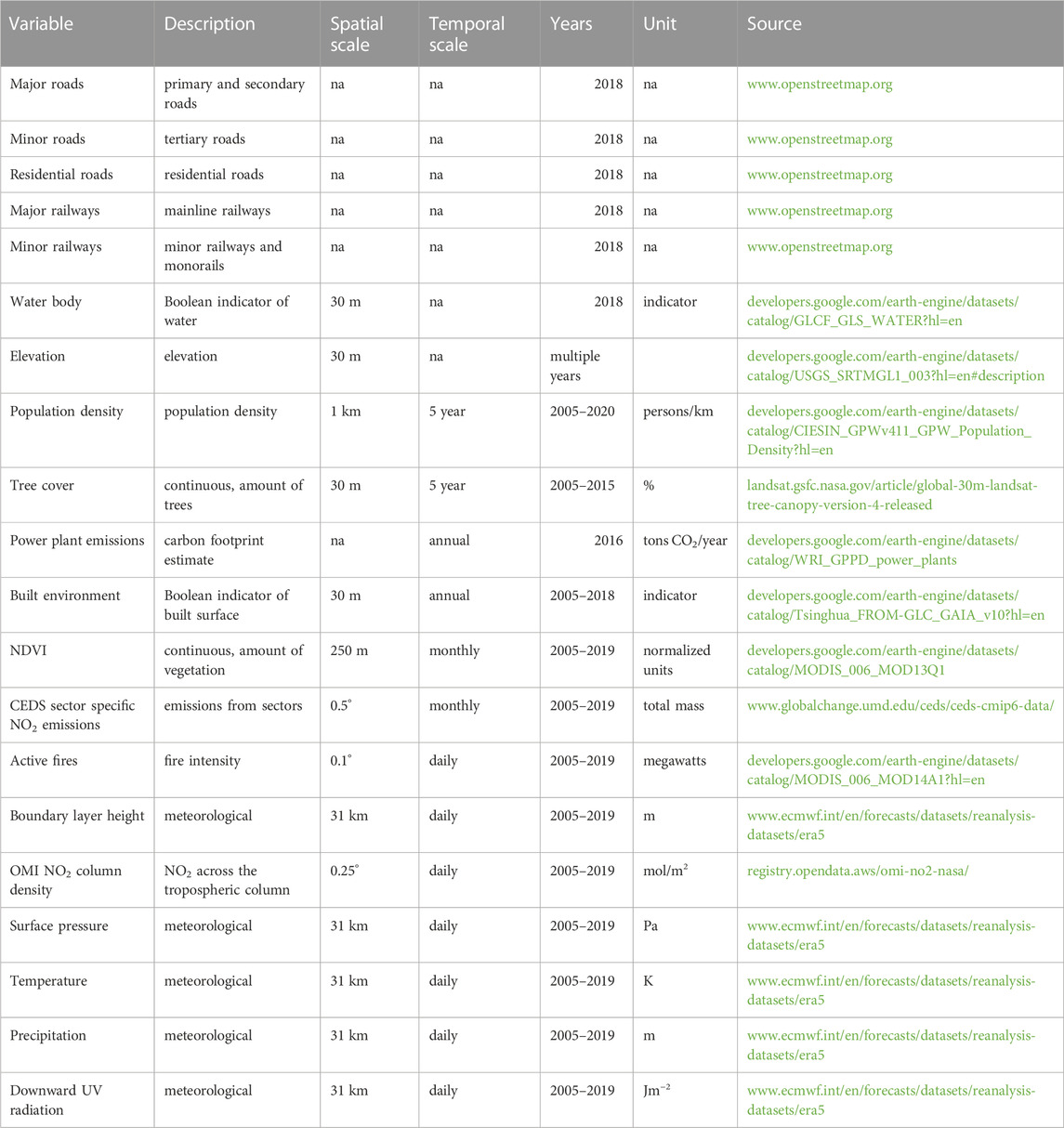
TABLE 1. Predictor variables derived for 8,250 air monitor locations, ordered by temporal resolution available.

Data were downloaded at the temporal resolution listed in Table 1 and for each fine-scale land use characteristic, multiple buffer variables were created, ranging from 50 m to 20 km in radius. Buffers in this study consisted of unweighted averages of land use characteristics within a set distance, such as average percent tree coverage within a circle that has a 200 m radius (i.e., 200 m buffer). Buffer variables and point estimates were calculated using Python 3.8.8 scripts written for automated analysis in ArcGIS Pro 2.8.0. Python scripts are available at https://github.com/larkinandy/LUR-NO₂-Model.

The temporal scale of variable predictors varied substantially based on availability. Road and railway networks were extracted from an August 2018 snapshot of the OpenStreetMap (OSM) geodatabase. We reclassified OSM road and railway networks into the following categories: Major roads were derived from OSM motorways, motorway links, trunks, trunk links, primary, and secondary roads and links. Minor roads were derived from OSM tertiary roads and tertiary road links. Residential roads were derived from OSM residential roads and residential road links. Other OSM road classifications (e.g., service roads and bridleways) were excluded. Major railways were derived from OSM mainline railways, and minor railways were derived from OSM light rail and monorails. Other predictors were available for temporal scales of 5 years, annually, monthly, or daily for our study period of 2005–2009.

Daily temporal variables included NO₂ tropospheric column density measurements and meteorological data. Daily NO₂ tropospheric column density measurements from the Ozone Monitoring Instrument (OMI) version 4.0 (Lamsal et al., 2021) were downloaded from NASA and linked to each OpenAQ monitoring station location. Measurements were preprocessed by NASA with a screen for snow cover, cloud fraction <30%, and data unaffected by an instrument obstruction called the row anomaly. Monthly averages were calculated if 25% of the daily averages were valid, and annual averages were calculated if 25% of the daily averages within the year and 1 monthly average within each quarter were valid. This screening will disproportionately affect polar and cloudy regions and have no effect on areas with climatologically clear skies. For meteorology, hourly boundary layer height, precipitation, surface temperature, and near surface atmospheric pressure predictions generated by the European Centre for Medium-Range Weather Forecasts (ECMWF) Reanalysis Model v5 (ERA5) were downloaded from the ECMWF database. Daily averages (12a.m.–11p.m. local time) were calculated after adjusting for local time zones.

2.2 Statistical analysis

Daily LUR models were developed using Lasso variable selection (glmnet package in RStudio, v. 1.4.1106). Regularization algorithms such as Lasso and ridge regression are preferred over stepwise regression when predictor variables are highly correlated (e.g., when the set of predictor variables includes multiple road density metrics) (Larkin et al., 2017; Chen et al., 2019). We chose to use Lasso rather than ridge regression to eliminate non-significant predictor variables and thus increase the ease of model interpretation (Larkin et al., 2017; Chen et al., 2019). Candidate variables considered during Lasso selection are shown in Table 1. The list of predictor variables selected by Lasso are discussed in Section 3.2.2.

Air monitor records were weighted by geographical and seasonal coverage during Lasso regression. Air monitor network coverage from 2005–2019 varied dramatically across the globe and between seasons. We used weights to account for the different global and season coverage of the available NO₂ monitoring data, to better model global NO₂ concentrations and predictors. In general, daily air monitor records from continents with extensive spatial and/or temporal coverage or from seasons with greater coverage were weighted less than air monitor records from continents with spare networks and/or minimal historical coverage. Supplementary Figure S1 describes the weighting method used. Parameters for Lasso variable selection include standardizing independent variables (standardization = True), selecting variables to minimize mean-squared error (type.measure = ’mse), and forcing the direction of variable coefficients to conform to a-priori hypotheses (lower.lim = 0). The lasso model with a lambda cross-validation score of one standard deviation from the minimum cross-validation score was selected as the model of choice to favor model simplification and inference over model prediction (s = lambda.1 se). To reduce multicollinearity, multiple buffer sizes of the same land use classification were only allowed in the final model if the radius of the larger buffer size was at least five times greater than the smaller buffer sizes. Predictor variables were included in the final model if they significantly reduced the mean squared error of model predictions (p < 0.05), increased adjusted R² either globally or within one or more continental regions by 1 percent or more, exhibited variance inflation factors less than 5 for at least one region and less than 10 for all regions.

To evaluate the final model performance, we calculated root mean squared error (RMSE) mean absolute error (MAE), adjusted R-squared (Adj. R²), mean percent bias (MB) and mean absolute bias (MAB) for the entire global dataset as well as each continental region. Leave 10% out cross-validation was performed, in which 10% of the monitors from each continental region were randomly sampled into a testing dataset, with the remaining 90% combined to create the model training dataset. Cross-validation was repeated in a bootstrap fashion 10,000 times to generate cross-validation estimates of RMSE, MAE, Adj. R², MB, and MAB both globally and within each continental region.

In chronic health studies, exposure estimates are often aggregated to monthly or annual averages to better capture seasonal and chronic NO₂ exposure trends. To test the performance of model aggregations, we derived monthly and annual averages of daily model predictions and compared them to monthly and annual averages of air monitor measurements. We also created a separate LUR model using annual rather than daily air monitor records and predictor variables and compared the performance of the annual and daily NO₂ models in predicting annual NO₂ concentrations.

In our previous 2010–2012 model (Larkin et al., 2017), RMSE and MB were greater in rural vs. urban areas. To test model performance across urban development levels, we identified urban development levels at air monitor locations using the Global Human Settlement layer (Corbane et al., 2018) and stratified daily, monthly, and annual cross-validation by urbanicity.

To test the utility of a global daily LUR model, we extracted daily 2012 NO₂ estimates for four hospitals in four hemispheres and calculated summary statistics and percent missing data. We also generated unweighted 30-day moving averages to compare daily predictions with monthly trends.

All of the R scripts used to create the LUR models, perform model performance, and perform sensitivity analyses are available at https://github.com/larkinandy/LUR-NO2-Model.

3 Results

3.1 Global NO₂ database

The geographical distribution of NO₂ annual averages are shown in Figure 1. Summary statistics for daily NO₂ averages stratified by region are shown in Table 2. More than 5.7 million days of valid measurements were collected from 8,250 air monitor locations. Air monitor coverage is greatest in Asia, Europe, and North America and sparse in Oceania, South America, and Africa. Annual concentrations range from 0 to 59 ppb (mean = 11.8), while daily concentrations range from 0 to 249 ppb (mean = 11.7). Mean daily concentration is noticeably lower in Oceania (4 ppb) in comparison to other regions (9–13 ppb). Daily standard deviation is likewise lower in Oceania (4 ppb) compared to other regions (9–11 ppb).

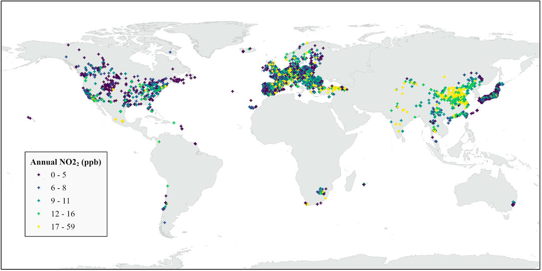
FIGURE 1. Global distribution of NO₂ air monitor and annual NO₂ concentrations (2005–2019). For air monitors with multiple years of measurements the most recent annual average is shown.

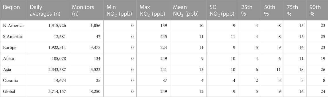
TABLE 2. NO₂ air monitor summary statistics (2005–2019), stratified by region.

3.2 Global LUR model

3.2.1 Model performance

Global NO₂ predictions are shown in Figure 2 for the final global LUR model. Cross-validation performance is shown in Table 3. See Supplementary Figure S3 for a closer look at model predictions below 5 ppb. Additional performance metrics are available in Supplementary Table S5. In 10% cross-validation, the regression model performance is 47% adjusted R² for daily, 59% adjusted R² for monthly, and 63% adjusted R² for global annual NO₂ predictions. Similarly, RMSE is greatest for daily predictions (6.8 ppb) and smallest for annual predictions (4.4 ppb). Regionally, daily adjusted R² ranged from 10% (Oceania) to 57% (North America). In general, model performance improved in each region when aggregating daily predictions to monthly and annual averages. Except for Oceania, annual adjusted R² ranged from 49% to 66%. Adjusted R² for Oceania is just 2% due to limited measured NO₂ variation in our dataset.

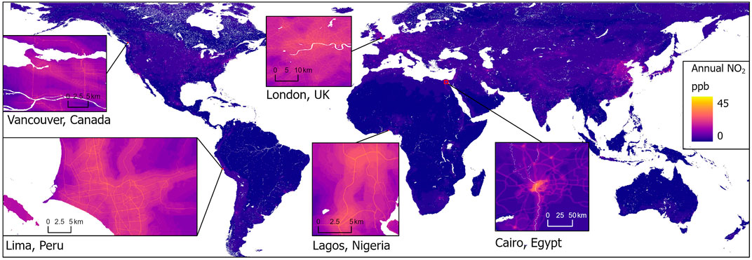
FIGURE 2. Global NO₂ model predictions for the year 2018. Inserts of select cities for each continental region demonstrate within city variation of model predictions.

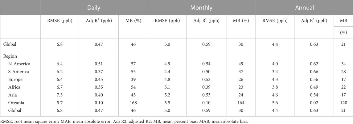
TABLE 3. Cross-validation model performance at estimating daily, monthly, and annual NO₂ concentrations.

3.2.2 Model structure

Predictor variables and contributions to model performance are shown in Table 4. Predictor variables include satellite based NO₂ estimates (OMI), meteorological conditions (temperature, atmospheric pressure), land use characteristics with positive coefficients (major, minor, and residential roads, population density) and land use characteristics with negative coefficients (tree cover, water body). The most significant variable is major roads within 50 m. Buffer sizes range from 50 m (major roads) to 20 km (water body). Major roads and OMI each consistently explain more than 5% of the NO₂ variation both globally and within all regions. However, the importance of other model variables varied between regions. For example, built up environment explains 12% of the NO₂ variation within Africa, but only 1.6% globally. Similarly, atmospheric pressure explains 5.1% of the NO₂ variation in South America, but less than 0.1% globally.

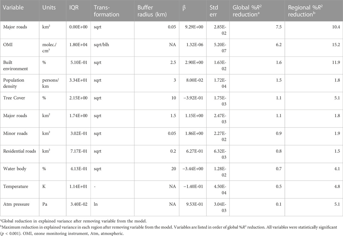
TABLE 4. Global LUR model structure.

Variables in the model with daily temporal resolution include OMI, temperature, and atmospheric pressure. The built up environment variable has annual resolution, while the tree cover and population density variables were updated every 5 years. Road networks and water body predictors were derived from a single time point and do not capture changes over time.

3.2.3 Spatial and temporal distribution

Figure 3 illustrates the different temporal predictors of the final model with January, July, and annual 2011 averages for Delhi, India. Delhi was selected as an example because of its heterogeneity in land use characteristics, seasonal variation in air pollutant concentration (Sharma et al., 2010), and because it iss a frequently used location for evaluating air pollutant modeling methods (Sharma et al., 2010; Karn et al., 2011; Larkin et al., 2017), thus facilitating inter-model comparisons. Also shown in Figure 3 is the 3-year 2010–2012 average predictions from a previously published LUR model developed with similar methodology and predictor variables (Larkin et al., 2017). In general, the spatial distribution of NO₂ is similar for both monthly and annual averages. Concentrations are greatest in areas with dense population density and built up environment (Eastern Delhi) and alongside major road networks. While spatial patterns are consistent across the year, the magnitude of predicted NO₂ concentrations differs between months and the annual average. Predicted NO₂ levels are noticeably above and below the annual average in January and July, respectively, in agreement with seasonal trends of NO₂ lifetime in the Northern Hemisphere (Karn et al., 2011). In comparison to 2010–2012 model published by Larkin et al. (2017), inclusion of minor and residential roads in the present model adds NO₂ traffic-related gradients outside of the dense urban core.

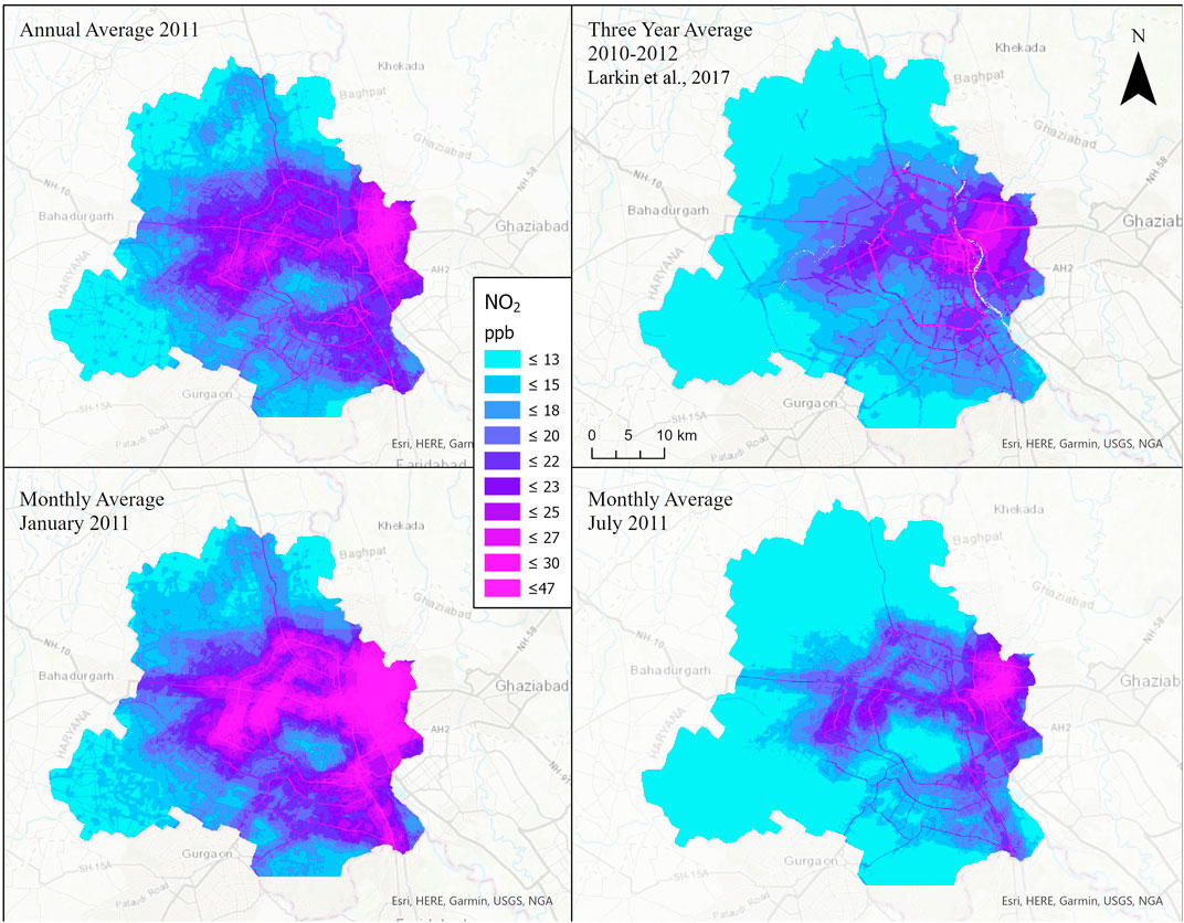
FIGURE 3. Comparison of NO₂ estimates across Delhi, India. Top left: Annual 2011 averages of daily model predictions. Bottom left and right: Average model predictions for January and July 2011, respectively. Top right: 3 year 2010–2012 average predictions from a previously published global NO₂ land use regression model using similar predictor variables (Larkin et al., 2017).

3.3 Sensitivity analysis

Cross-validation performance of annual predictions derived from daily and annual NO₂ LUR models are shown in Table 5 (see Section 2.2 for more details about the annual NO₂ LUR model). Globally, model performances are similar. RMSE and MAE differ by 0.1 ppb, MB, and MAB differ by 1% and 2%, respectively, and Adj R² differs by 0.02. Regionally, the daily and annual models differ the most in South America (RMSE and Adj R² are 1.2 ppb lower and 0.09 higher, respectively for the daily model) and Oceania (RMSE is 0.9 ppb lower for the annual model, while Adj R² is equal between the daily and annual models). In general, results suggest the error in annual averages of daily model predictions does not significantly differ from predictions generated by an LUR model optimized for predicting annual concentrations.

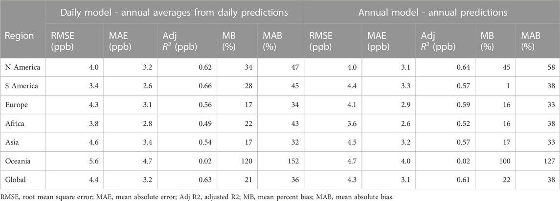
TABLE 5. Cross-validation performance of daily and annual LUR model performances in predicting annual NO₂ concentrations.

Table 6 shows cross-validation model performance stratified by urbanicity (urban vs. rural). RMSE is lower in rural settings vs. urban settings. For example, annual RMSE is 4.6 ppb and 2.9 ppb for urban and rural air monitors, respectively. However, RMSE relative to mean concentrations are greater in rural than urban air monitors. For example, the annual mean:RMSE ratio is 2.8 and 1.8 for urban and rural air monitors, respectively.

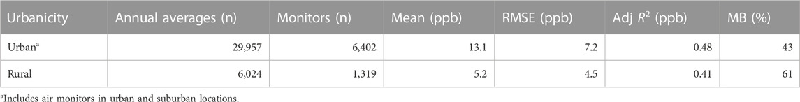
TABLE 6. Cross-validation performance annual LUR model performances stratified by urbanicity.

Daily model predictions and moving average trendlines for four hospitals are shown in Figure 4. We chose these four hospitals because they are within well-known urban centers, distributed across the four hemispheres, and have published latitude/longitude coordinates with spatial resolution greater than or equal to model estimates. Mean concentrations are greatest in Dhaka (28.6 ppb) and smallest in Cape Town (12.0 ppb). Standard deviation is greatest in Buenos Aires (2.4 ppb). Thirty-day trends demonstrate increased NO₂ concentrations in winter months (December—February in New York City and Dhaka, and June—August in Buenos Aires and Cape Town). Percent days with coverage ranges from 49.7% in New York City to 59.8% in Dhaka. Missing days are due to missing OMI columnar estimates.

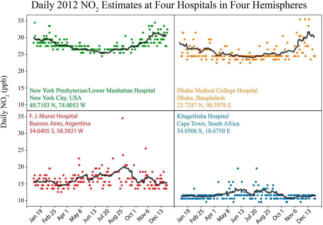
FIGURE 4. Daily predictions for four urban hospitals across the globe. Figures also include an unweighted 30 days moving average trendline in black.

4 Discussion

We collected 5.7 million daily averages from 8,250 air monitors (approximately 691 daily averages per monitor) and developed a daily global NO₂ model at 50 m resolution. The model captured 47% of daily, 59% of monthly, and 63% of annual global NO₂ variation. Predictor variables for the model are available from 2005 to the present, which allows for retrospective exposure estimates for global burden of disease studies as well as in long running epidemiological cohorts, particularly in developing countries where NO₂ data and models are limited or not available.

The model structure consists of variables with a range of spatial and temporal resolutions that correspond to NO₂ emission sources and patterns. Road networks make up variables from 50 to 200 m in resolution. Population density and built up environment variables capture moderate spatial resolutions (2.5 and 3 km, respectively), while OMI, meteorological variables, and protective land use characteristics such as water and trees capture more regional NO₂ distributions (10 km–31 km). While OMI and meteorological variables might have coarse spatial resolutions, these variables have daily temporal resolution and thus are responsible for the model’s ability to capture day to day variation in NO₂ concentrations.

Several model variables contributed little to global variation but were highly significant to capturing regional NO₂ variation. For example, built environments explained 11.9% of NO₂ variation in Africa (specifically, South Africa), but only 1.6% of the global NO₂ variation. This highlights one of the challenges of developing large scale LUR models, in which associations between predictors and outcomes may differ when stratified by sub-regions compared to examining unstratified associations. This trade-off has been highlighted in other studies examining global NO₂ modelling (Larkin et al., 2017). Other variables such as road networks may have strong associations across all subregions, but the magnitudes of those associations may differ due to regional factors such as fleet composition, traffic levels and congestion, and emission standards. We included Community Emissions Data System (CEDS) (McDuffie et al., 2020) Sector Specific NO_x Emissions, including surface transportation emissions, in our list of candidate variables (Table 1). However, none of the CEDS estimates were selected by the Lasso algorithm. Future models may benefit from emission inventories with higher spatial resolution.

Air monitor records are disproportionately greater in North America, Europe, and Asia. To mitigate, we weighted air monitor records to adjust for disproportionate spatial and temporal representation. Still, confidence in model predictions is greatest in these regions with greater coverage. The spatial extent of air monitors in Africa, South America, and Australia represents a small percentage of these continental regions and may therefore have limited generalizability across all respective countries or territories. Regression models were fitted to minimize mean square error (MSE), the square of RMSE, and daily RMSE of continental regions with large numbers of daily records (6.4–7.3 ppb) is surprisingly greater than RMSE of regions with small numbers of daily records (5.7–6.7 ppb). This may be due to the higher absolute concentrations in areas where there are many monitors. In non-polluted areas with lower absolute concentrations, RMSE of ∼6 ppb can still represent percent errors exceeding 100%. Despite this, for global studies which aim to standardize RMSE as equally as possible across multiple continents, the weighted modeling approach implemented in this model appears to work well. However, while RMSE is evenly distributed across regions, MB is noticeably higher and Adj. R² (0.10) is noticeably lower for Oceania than other regions. Poor MB and Adj. R² performance in Oceania is in partly attributable to the inclusion of a small set of NO₂ monitoring data from Australia that was available in OpenAQ. The mean and standard deviation of daily concentrations in Oceania is low (4 and 4 ppb, respectively) and well below global values (9 and 11 ppb). The smaller daily averages lead to larger MB when RMSE is the same. For example, an RMSE of 2 ppb with an air monitor record of 2 ppb is a 100% MB, while an RMSE of 2 ppb with an actual concentration of 20 ppb is 10% MB. In a larger and more geographically diverse external validation dataset of annual Oceania air monitor measurements (Larkin et al., 2017), model performance in Oceania is noticeably better and similar to North America and Europe (Table 7).

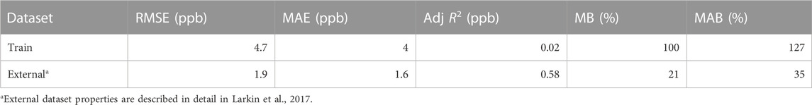
TABLE 7. Comparison of model performance in oceania training and external validation datasets.

Compared to monthly or annual models, daily NO₂ estimates may be more susceptible to meteorological confounding, in which both OMI coverage and NO₂ concentrations are associated with cloudy weather. Our model does not make predictions for days with missing OMI values, and therefore has the same spatial-temporal coverage as columnar OMI. In our sensitivity analysis we used predictor variables selected by Lasso to develop new monthly and annual NO₂ models and compared these model cross-validation performances to monthly and annual averages of the daily model predictions. Differences between models were within 2%, which is within the random variation observed between bootstrap cross-validation instances. The geographic variables included in the monthly and annual model (Supplementary Table S4) were similar to the daily model, suggesting these are consistently the most important predictors of geographical NO₂ patterns. These comparisons suggest using the daily model for deriving monthly and annual exposures does not increase model error. Users should evaluate the percent missing coverage for their date(s) and region(s) of interest and might consider using statistical methods such as moving averages (Figure 4) to fill in missing days. However, it also suggests the additional computational costs of deriving daily results is not needed unless health studies can leverage daily exposure estimates to refine their health analyses. For acute studies such as hospital admissions following extreme exposures, daily estimates can be more useful than monthly or annual estimates.

Sensitivity models suggest model performance differs between urban and rural areas. Model predictions for rural locations have greater error than their respective urban counterparts, which is not surprising given the limited number of rural air pollution monitors available. For studies with rural participants, we recommend either using annual rather than daily or monthly model predictions or restricting analyses to urban and suburban participants.

Our NO₂ model has several limitations that should be considered when applying the model. First, model predictions are dependent on valid daily OMI measurements. We did not evaluate or exclude air monitor records based on air monitor sampling quality as most records from OpenAQ are semi-real time and do not include air monitor sampling details. In addition to meteorological limitations such as cloud cover, the number of valid daily pixel measurements from the OMI sensor on the Aura satellite has gradually been decreasing over time due to an instrument obstruction first noticed in 2007 (Schenkeveld et al., 2017). From 2018 onwards, measurements are available from the TROPOMI instrument, with substantially higher spatial resolution compared with OMI. Future studies would benefit from an adaptation of this model using TROPOMI rather than OMI as the satellite-based measure of columnar NO₂. Second, this model relies on road networks as a secondary indicator for vehicle emissions. Travel patterns have significantly changed since the onset of the COVID-19 pandemic and studies have demonstrated significant declines in NO₂ during lock-down periods (Hoang et al., 2021). We therefore restricted our model training and performance analysis to the years 2005–2019. Future research should examine potential long-term changes in travel behavior and how this impacts NO₂ levels and patterns.

We created a daily global NO₂ model with 50 m spatial resolution, with coverage from 2005–2019. In bootstrap cross-validation, the model captured 47%, 59%, and 63% of daily, monthly, and annual variation in NO₂ concentrations. We will make these NO₂ model estimates available, which can be used to retrospectively estimate acute and chronic exposures for risk assessments (e.g., global burden of disease studies), for multi-national health studies, where measurements are ideally standardized across regions, and for studies in developing countries were NO₂ monitoring data or detailed models are not available. Interested epidemiologists should consider the strengths and limitations of the documented model, particularly with respect to the spatial and temporal extent and resolution of their cohort data (Yin et al., 2020).

Data availability statement

The raw data supporting the conclusion of this article are freely available from the sources listed in Table 1.

Author contributions

AL downloaded datasets, created and evaluated the model, and wrote the majority of the manuscript. SA was the PI on the project, provided insight and consulting into deriving spatio-temporal weights, and contributed to writing the manuscript. DG provided algorithms for screening satellite imagery and normalizing air monitor records. AM developed algorithms for weighting regions by urbanicity. MB consulted on regional weighting and wrote a large percentage of the manuscript discussion. PH contributed to evaluating model performance, finding air monitors in developing countries, and writing the introduction, results, and discussion sections of the manuscript.

Funding

This study was supported by grants from the Health Effects Institute and Bloomberg Philanthropies (research agreement 4977/20–11). SA, DG, and AM were also supported by a grant from NASA (grant no. 80NSSC19K0193).

Acknowledgments

We greatly appreciate the Canada National Air Pollution Surveillance Program (NAPS), European Topic Centre on Air and Climate Change, Japan Ministry of the Environment, OpenAQ, Mexico Ministry of the Environment, South African Air Quality Information System (SAAQIS), and US Environmental Protection Agency (EPA) for maintaining and updating publicly available air monitor measurement datasets.

Conflict of interest

The authors declare that the research was conducted in the absence of any commercial or financial relationships that could be construed as a potential conflict of interest.

Publisher’s note

All claims expressed in this article are solely those of the authors and do not necessarily represent those of their affiliated organizations, or those of the publisher, the editors and the reviewers. Any product that may be evaluated in this article, or claim that may be made by its manufacturer, is not guaranteed or endorsed by the publisher.

Supplementary material

The Supplementary Material for this article can be found online at: https://www.frontiersin.org/articles/10.3389/fenvs.2023.1125979/full#supplementary-material

References

Amini, H., Taghavi-Shahri, S. M., Henderson, S. B., Hosseini, V., Hassankhany, H., Naderi, M., et al. (2016). Annual and seasonal spatial models for nitrogen oxides in Tehran, Iran. Sci. Rep. 6 (1), 1–11. doi:10.1038/srep32970
Beckerman, B., Jerrett, M., Brook, J. R., Verma, D. K., Arian, M. A., and Finkelstein, M. M. (2008). Correlation of nitrogen dioxide with other traffic pollutants near a major expressway. Atmos. Environ. 42 (2), 275–290. doi:10.1016/j.atmosenv.2007.09.042
Chen, J., de Hoogh, K., Gulliver, J., Hoffmann, B., Hertel, O., Ketzel, M., et al. (2019). A comparison of linear regression, regularization, and machine learning algorithms to develop Europe-wide spatial models of fine particles and nitrogen dioxide. Environ. Int. 130, 104934. doi:10.1016/j.envint.2019.104934
Cohen, A. J., Brauer, M., Burnett, R., Anderson, H. R., Frostad, J., Estep, K., et al. (2017). Estimates and 25-year trends of the global burden of disease attributable to ambient air pollution: An analysis of data from the global burden of diseases study 2015. Lancet 389 (10082), 1907–1918. doi:10.1016/s0140-6736(17)30505-6
Cooper, M. J., Martin, R. V., McLinden, C. A., and Brook, J. R. (2020). Inferring ground-level nitrogen dioxide concentrations at fine spatial resolution applied to the TROPOMI satellite instrument. Environ. Res. Lett. 15 (10), 104013. doi:10.1088/1748-9326/aba3a5
Corbane, C., Florczyk, A., Pesaresi, M., Politis, P., and Syrris, V. (2018). GHS built-up grid, derived from Landsat, multitemporal (1975-1990-2000-2014), R2018A. Brussels, Belgium: European Commission, Joint Research Centre. doi:10.2905/jrc-ghsl-10007
Dickerson, R. R., Anderson, D. C., and Ren, X. (2019). On the use of data from commercial NOx analyzers for air pollution studies. Atmos. Environ. 214, 116873. doi:10.1016/j.atmosenv.2019.116873
Duncan, B. N., Lamsal, L. N., Thompson, A. M., Yoshida, Y., Lu, Z., Streets, D. G., et al. (2016). A space-based, high-resolution view of notable changes in urban NOxpollution around the world (2005-2014): Notable changes in urban noxpollution. J. Geophys. Res. Atmos. 121 (2), 976–996. doi:10.1002/2015JD024121
Dunlea, E. J., Herndon, S. C., Nelson, D. D., Volkamer, R. M., San Martini, F., Sheehy, P. M., et al. (2007). Evaluation of nitrogen dioxide chemiluminescence monitors in a polluted urban environment. Atmos. Chem. Phys. 7 (10), 2691–2704. doi:10.5194/acp-7-2691-2007
Goldberg, D. L., Anenberg, S. C., Kerr, G. H., Mohegh, A., Lu, Z., and Streets, D. G. (2021). TROPOMI NO2 in the United States: A detailed look at the annual averages, weekly cycles, effects of temperature, and correlation with surface NO2 concentrations. Earth’s Futur. 9 (4), e2020EF001665. doi:10.1029/2020EF001665
Hamra, G. B., Laden, F., Cohen, A. J., Raasachou-Nielsen, O., Brauer, M., and Loomis, D. (2015). Lung cancer and exposure to nitrogen dioxide and traffic: A systematic review and meta-analysis. Environ. Health Perspect. 123 (11), 1107–1112. doi:10.1289/ehp.1408882
Hoang, A. T., Huynh, T. T., Nguyen, X. P., Nguyen, T. K. T., and Lee, T. H. (2021). An analysis and review on the global NO2 emission during lockdowns in COVID-19 period. Energy Sources, Part A Recovery, Util. Environ. Eff. 1–21.
Jamali, S., Klingmyr, D., and Tagesson, T. (2020). Global-scale patterns and trends in tropospheric NO2 concentrations. Remote Sens. 12 (21), 3526. doi:10.3390/rs12213526
Karn, Vohra, Marais, E. A., Suckra, S., Kramer, L., Bloss, W. J., Sahu, R., et al. (2011). Long-term trends in air quality in major cities in the UK and India: A view from space. Atm. Chem. Phys. 21 (8), 6275–6296. doi:10.5194/acp-21-6275-2021
Khreis, H., Kelly, C., Tate, J., Parslow, R., Lucas, K., and Nieuwenhujisen, M. (2017). Exposure to traffic-related air pollution and risk of development of childhood asthma: A systematic review and meta-analysis. Environ. Int. 100, 1–31. doi:10.1016/j.envint.2016.11.012
Krotkov, N. A., McLinden, C. A., Li, C., Lamsal, L. N., Celarier, E. A., Marchenko, S. V., et al. (2016). Aura OMI observations of regional SO&lt;sub&gt;2&lt;/sub&gt; and NO&lt;sub&gt;2&lt;/sub&gt; pollution changes from 2005 to 2015. Atmos. Chem. Phys. 16 (7), 4605–4629. doi:10.5194/acp-16-4605-2016
Lamsal, L. N., Krotkov, N. A., Vasilkov, A., Marchenko, S., Qin, W., Yang, E. S., et al. (2021). Ozone Monitoring Instrument (OMI) Aura nitrogen dioxide standard product version 4.0 with improved surface and cloud treatments. Atmos. Meas. Tech. 14 (1), 455–479. doi:10.5194/amt-14-455-2021
Larkin, A., Geddes, J. A., Martin, R. V., Xiao, Q., Liu, Y., Marshall, J. D., et al. (2017). Global land use regression model for nitrogen dioxide air pollution. Environ. Sci. Technol. 51 (12), 6957–6964. doi:10.1021/acs.est.7b01148
Levelt, P., Joiner, J., Tamminen, J., Veefkind, J. P., Bhartia, P. K., Stein Zweers, D. C., et al. (2018). The ozone monitoring instrument: Overview of 14 Years in space. Atmos. Chem. Phys. 18 (8), 5699–5745. doi:10.5194/acp-18-5699-2018
Lu, M., Schmitz, O., de Hoogh, K., Kai, Q., and Karssenberg, D. (2020). Evaluation of different methods and data sources to optimise modelling of NO2 at a global scale. Environ. Int. 142, 105856. doi:10.1016/j.envint.2020.105856
McDuffie, E. E., Smith, S. J., O'Rourke, P., Tibrewal, K., Venkataraman, C., Marais, E. A., et al. (2020). A global anthropogenic emission inventory of atmospheric pollutants from sector-and fuel-specific sources (1970–2017): An application of the community emissions data System (CEDS). Earth Syst. Sci. Data 12 (4), 3413–3442. doi:10.5194/essd-12-3413-2020
Patton, A. P., Perkins, J., Zamore, W., Jevy, J. I., Brugge, D., and Durant, J. L. (2014). Spatial and temporal differences in traffic-related air pollution in three urban neighborhoods near an interstate highway. Atmos. Environ. 99, 309–321. doi:10.1016/j.atmosenv.2014.09.072
Rice, M. B., Ljungman, P. L., Wilker, E. H., Gold, D. R., Schwartz, J. D., Koutrakis, P., et al. (2013). Short-term exposure to air pollution and lung function in the Framingham Heart Study. Am. J. Respir. Crit. Care Med. 188 (11), 4092–1357. doi:10.1289/isee.2013.o-1-22-01
Richmond-Bryant, J., Owen, R. C., Graham, S., Snyder, M., McDow, S., Oakes, M., et al. (2017). Estimation of on-road NO2 concentrations, NO2/NOX ratios, and related roadway gradients from near-road monitoring data. Air Qual. Atmos Health 10, 611–625. doi:10.1007/s11869-016-0455-7
Schenkeveld, V. M., Jaross, G., Marchenko, S., Haffner, D., Kleipool, Q. L., Rozemeijer, N. C., et al. (2017). In-flight performance of the ozone monitoring instrument. Atmos. Meas. Tech. 10 (5), 1957–1986. doi:10.5194/amt-10-1957-2017
Sharma, S. K., Datta, A., Saud, T., Saxena, M., Mandal, T. K., Ahammed, Y. N., et al. (2010). Seasonal variability of ambient NH3, NO, NO2 and SO2 over Delhi. J. Environ. Sci. 22 (7), 1023–1028. doi:10.1016/s1001-0742(09)60213-8
Sun, K., Zhu, L., Cady-Pereira, K., Chan Miller, C., Chance, K., Clarisse, L., et al. (2018). A physics-based approach to oversample multi-satellite, multi-species observations to a common grid. Atmos. Meas. Tech. Discuss. 11 (12), 1–30. doi:10.5194/amt-2018-253
VanGeffen, J., Eskes, H. J., Boersma, K. F., Maasakkers, J. D., and Veefkind, J. P. (2021). TROPOMI ATBD of the total and tropospheric NO2 data products.
Wang, Z., Peng, J., Liu, P., Duan, Y., Huang, S., Wen, Y., et al. (2020). Association between short-term exposure to air pollution and ischemic stroke onset: A time-stratified case-crossover analysis using a distributed lag nonlinear model in shenzhen, China. Environ. Health. 19 (1), 1–12. doi:10.1186/s12940-019-0557-4
Yin, P., Brauer, M., Cohen, A. J., Wang, H., Li, J., Burnett, R. T., et al. (2020). The effect of air pollution on deaths, disease burden, and life expectancy across China and its provinces, 1990–2017: An analysis for the global burden of disease study 2017. Lancet Planet. Health 4 (9), e386–e398. doi:10.1016/s2542-5196(20)30161-3
Keywords: NO2, land use regression (LUR), global, daily, air pollution
Citation: Larkin A, Anenberg S, Goldberg DL, Mohegh A, Brauer M and Hystad P (2023) A global spatial-temporal land use regression model for nitrogen dioxide air pollution. Front. Environ. Sci. 11:1125979. doi: 10.3389/fenvs.2023.1125979
Received: 16 December 2022; Accepted: 03 April 2023;
Published: 18 April 2023.
Edited by:
Rui Li, Tsinghua University, ChinaReviewed by:
Vijay Bhaskar Bojan, Madurai Kamaraj University, IndiaAna Prados, University of Maryland, Baltimore County, United States
Copyright © 2023 Larkin, Anenberg, Goldberg, Mohegh, Brauer and Hystad. This is an open-access article distributed under the terms of the Creative Commons Attribution License (CC BY). The use, distribution or reproduction in other forums is permitted, provided the original author(s) and the copyright owner(s) are credited and that the original publication in this journal is cited, in accordance with accepted academic practice. No use, distribution or reproduction is permitted which does not comply with these terms.
*Correspondence: Andrew Larkin, larkinan@oregonstate.edu