

Integrating eDNA and citizen science observations to model distribution of a temperate freshwater turtle near its northern range limit
- Published
- Accepted
- Received
- Academic Editor
- Xavier Pochon
- Subject Areas
- Biodiversity, Ecology, Zoology, Climate Change Biology, Freshwater Biology
- Keywords
- Species distributions, Niche models, Freshwater turtle, Environmental DNA, Community science, Range limits, Climate change, SDMs
- Copyright
- © 2023 Feng and Lougheed
- Licence
- This is an open access article distributed under the terms of the Creative Commons Attribution License, which permits using, remixing, and building upon the work non-commercially, as long as it is properly attributed. For attribution, the original author(s), title, publication source (PeerJ) and either DOI or URL of the article must be cited.
- Cite this article
- 2023. Integrating eDNA and citizen science observations to model distribution of a temperate freshwater turtle near its northern range limit. PeerJ 11:e15120 https://doi.org/10.7717/peerj.15120
Abstract
Background
To determine species distributions and the factors underlying them, reliable occurrence data are crucial. Assembling such data can be challenging for species with cryptic life histories or that occur at low densities.
Methods
We developed species-specific eDNA protocols, from sampling through data interpretation, to detect the common musk turtle (Sternotherus odoratus) and tested whether eDNA occurrences change our understanding of the species distribution and the factors that shape its northern range limit. We used Species Distribution Models (SDMs) with full parameter optimization on citizen science observations of S. odoratus in Southern Ontario alone and together with eDNA occurrences.
Results
Our eDNA protocol was robust and sensitive. SDMs built from traditional observations and those supplemented with eDNA detections were comparable in prediction accuracy. However, models with eDNA detections suggested that the distribution of S. odoratus in Southern Ontario is underestimated, especially near its northern range limit, and that it is shaped by thermal conditions, hydrology, and elevation. Our study underscores the promise of eDNA for surveying cryptic aquatic organisms in undocumented areas, and how such insights can help us to improve our understanding of species distributions.
Introduction
A primary goal of ecology and conservation biology is to determine the distributions of organisms and understand the factors that shape them. Reasons for why a species persists in some regions but is absent from others are complex as species distributions are influenced by multiple factors, including abiotic factors (e.g., precipitation, temperature), biotic interactions, and dispersal ability (Soberón & Peterson, 2005). Critical to understanding species distributions are comprehensive occurrence data, which can comprise presences and absences, or presences-only (MacKenzie et al., 2018). The traditional sources for presence data include museum records, dedicated surveys, and increasingly, online databases that contain citizen science observations (Newbold, 2010; Tiago, Pereira & Capinha, 2017). However, such online databases can be taxonomically biased, and skewed to data from regions with higher human populations or recreational activities (Titley, Snaddon & Turner, 2017), potentially leading to inaccurate descriptions of species ranges and habitat preferences (Araújo & Guisan, 2006).
Various methods have been used for assembling occurrence data, with their effectiveness depending particularly on species life histories (e.g., sociality, diurnality). Visual and auditory surveys are common sources for occurrence records (Gibb et al., 2019; Winship et al., 2020), as well as seining and trawling for fish (Porter, Rosenfeld & Parkinson, 2000), mist netting for birds and bats (Chandler et al., 2018; Scherrer, Christe & Guisan, 2019), and live trapping for mammals (Sofaer et al., 2019). New tools, including trail cameras, geolocators, satellite tracking, and environmental DNA (eDNA), are proving fruitful for deriving occurrence records (Coxen et al., 2017).
eDNA is increasingly featured in ecology, conservation biology (Beng & Corlett, 2020), and epidemiology (Ogden, 2021). eDNA surveys are now widely used to assess species occurrences, especially in aquatic systems (Rees et al., 2014; Seymour, 2019). Single species eDNA detection techniques such as quantitative PCR (qPCR) and digital PCR can supplement traditional survey data (Wineland et al., 2019). Such eDNA datasets have been used in invasive species monitoring (Sepulveda et al., 2020), species conservation (Takahara et al., 2020), quantification of biotic assemblages (West et al., 2020), and establishing range extensions (Gorički et al., 2017; Nardi et al., 2020). eDNA surveys may be more cost-effective than traditional methods, easier to replicate, and more sensitive for detection of rare or cryptic species (Muha et al., 2017; Olson, Briggler & Williams, 2012).
To infer range limits and habitat suitability for species, describe their ecological niches, and project their distribution over space and time, species distribution models (SDMs) are often used, including those generated using a Maximum Entropy algorithm (MaxEnt. Phillips, Anderson & Schapire, 2006). With the promise of overcoming some of the deficiencies of traditional survey methods, eDNA data have been recently brought into such SDMs (Carraro et al., 2018; Neto et al., 2020; Schmelzle & Kinziger, 2016), though such applications have yet to be robustly tested. Here, for a small freshwater North American turtle we ask whether targeted eDNA sampling changes our understanding of the environmental factors that underlie its distribution or extends its known geographical range.
The common musk turtle (Sternotherus odoratus) is an excellent candidate to test the value of eDNA surveys for SDMs. Ranging from Florida to Southern Ontario and Quebec, and west to Wisconsin and central Texas, it occupies shallow and slow-moving waterbodies with soft substrates (Dreslik & Phillips, 2005). While widespread, S. odoratus is difficult to observe because it is often crepuscular (Ernst, 1986). Sternotherus odoratus mostly basks just below the water surface often within patches of aquatic vegetation making visual detection from above the surface challenging. Overland movement of the turtle is uncommon, and its home ranges are probably confined to one waterbody (Ernst & Lovich, 2009), making incidental observations less likely. The known range of S. odoratus in Canada includes scattered locales across southern and central Ontario, and a small portion of western Quebec, with the current suspected northern range limit along the southern edge of the Canadian Shield (Fig. 1A; COSEWIC, 2012). Additional challenges near the northern range limit include a shorter active season (April to September) than at more southerly latitudes (e.g., year-around in Florida), and human presence that diminishes rapidly northward from the Canada-USA border leading to fewer overall citizen science observations. We thus suspect that the northern range limit of S. odoratus is underestimated and our understanding of its habitat usage is incomplete.
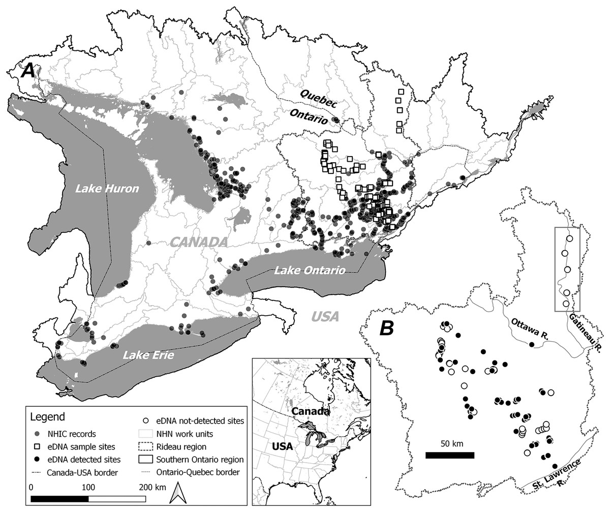
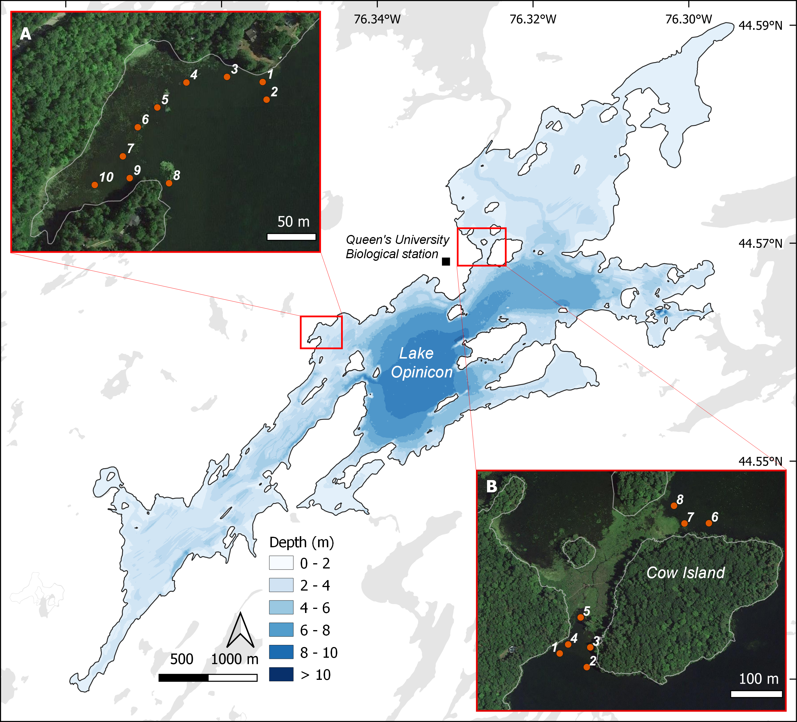
Figure 1: Study area, observational occurrences and eDNA sampling sites.
Two modelling regions, Southern Ontario (A) and Rideau (B) are marked by black solid and dotted lines, with the boundaries determined by combining relevant National Hydro Network (NHN) work units (grey dotted lines). In (A) observational occurrences retrieved from the Natural Heritage Information Centre (NHIC) and eDNA surveys sites are indicated by solid circles and open squares, respectively. In (B) eDNA detections and non-detections are marked with solid circles and open circles, respectively. Further, eDNA sites along the Gatineau River (see Methods) well beyond the northern range limit are indicated within the rectangle.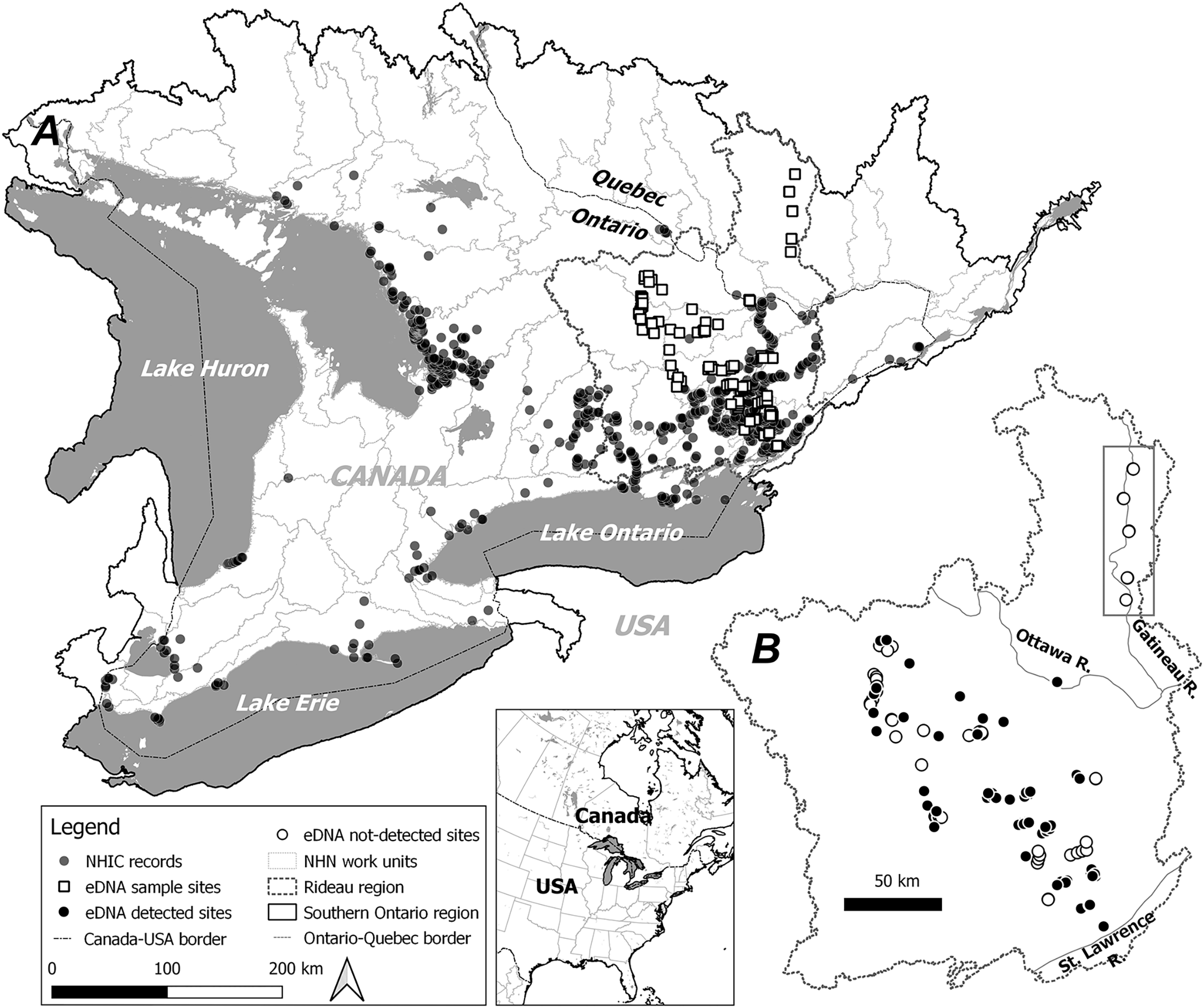
To address this deficit, we developed eDNA protocols to survey S. odoratus near and beyond its northern range limits and modelled its distribution with citizen science observations alone and with citizen science combined with eDNA occurrence data. We asked: (1) Can eDNA surveys reliably detect musk turtles? (2) How do additional eDNA occurrences change the outcomes of niche modelling? (3) Will eDNA data expand its range, especially towards its currently diagnosed range limit? (4) What environmental factors limit S. odoratus at its northern range boundary? To address these questions, we first examined the robustness and sensitivity of a new eDNA qPCR assay to detect S. odoratus in natural environments. We then modelled the distribution of S. odoratus using MaxEnt, with and without eDNA occurrences at two geographical scales, and compared the niche models built from different datasets. Finally, we evaluated all models to determine the underlying factors that may contribute to the northern range limit of S. odoratus.
Materials and Methods
Occurrence data and eDNA surveys for S. odoratus
We obtained occurrence records for S. odoratus from the Natural Heritage Information Centre (NHIC. Retrieval date: 2020-11-01. Fig. 1A), a public repository that houses data from dedicated surveys and citizen science observations with curation. In total 5,629 observations were available from 1913 to the present, with most from the past 20 years (Fig. S1).
Based on the current known species distribution, we conducted eDNA surveys in southeastern Ontario only, covering areas where S. odoratus is known to occur and areas where it has never been formally recorded, including north of its reported range limit. From May through August 2017 and 2018, we surveyed 145 sites starting from the eastern terminus of Lake Ontario extending approximately 200 km northwest, with additional sites along the Gatineau River reaching a 46.5°N latitude (Fig. 1B). Surveyed sites included shallow aquatic environments like littoral zones of lakes and rivers, slow-moving creeks and streams, and large wetlands, all potential musk turtle habitats (Dreslik & Phillips, 2005; COSEWIC, 2012). Because eDNA shedding rates can vary markedly among organisms (Andruszkiewicz Allan et al., 2021), and animals with hard keratinized integuments probably shed less DNA (Nordstrom et al., 2022), we wished to test the ability of our eDNA assay to detect musk turtles. Thus, we undertook intensive sampling in the mid-sized Lake Opinicon (44.5°N, 76.3°W), approximately 50 km north of the city of Kingston, ON, where S. odoratus are known to occur (Larocque et al., 2012) and vary in density in different parts of the lake.
At each survey site, 1 L of water was taken approximately 0.5 m below the surface using a sterile Nalgene bottle. Each water sample was filtered on-site using a field peristaltic pump (Waterra, Mississauga, ON, Canada) with 1.2-micron Isopore™ polycarbonic membranes (Sterlitech, Auburn, WA, USA) housed in a sterile 47 mm in-line filter holder (Pall, New York, NY, USA). The filters were stored in 2 mL Eppendorf tubes with 500 µL 2% (w/v) fresh cetyltrimethylammonium bromide extraction (CTAB) buffer (Clarke, 2009). The filtration apparatus was sterilized with 5% bleach solution and then rinsed with distilled water between sampling events. On each survey day, 1 L of distilled water was also filtered following the same method to serve as a blank negative field control. All filters were transported to Queen’s University on dry-ice and extracted within 48 h using a phenol-chloroform method in a dedicated fume hood (Article S1).
qPCR detection for S. odoratus
We developed a probe-based qPCR assay for musk turtles. The primer and TaqMan™ MGB probe were designed using PrimerExpress (v3.0; Applied Biosystems, Waltham, MA, USA) for the mitochondrial cytochrome b (cytb) gene. The primer set was tested for non-target organisms using Primer BLAST (https://www.ncbi.nlm.nih.gov/). More specifically we targeted a region where co-occurring turtles species exhibit many mismatches (details in Table S1). The qPCR amplifications were performed using a CFX96 Touch™ Real-Time PCR (Bio-Rad, Hercules, CA, USA) with reaction cocktails containing: 10 μL SensiFAST™ probe NO-ROX mix (Bioline, Tauton, MA, USA), 400 nM forward and reverse primer, 200 nM TaqMan probe, 10 μg Bovine Serum Albumin, 4 μL DNA template with reverse osmosis H2O added to a final volume of 20 μL. The cycling profile was: 2 m of at 95 °C, 45 cycles of two-step amplification with 10 s of denaturation at 95 °C and 20 s of annealing/extension at 60 °C. All assays were done in triplicate (i.e., three technical replicates) in 96-well PCR plates (BioRad, Hercules, CA, USA). For each plate, we established a standard curve using a seven-point ten-fold dilution series from a quantified plasmid solution with the target amplicon (Article S2). To control for potential aerosol contamination, we prepared all qPCR assays in a dedicated Edgegard™ laminar flow hood (Baker, Sanford, ME, USA) and included triplicate non-template controls for each plate. To test the specificity and detection limit of our eDNA assay for S. odoratus, we tested our primer and probe set against genomic DNA extracted from other co-occurring turtles (Table S1), and on eDNA samples from two locations in Lake Opinicon (Fig. S2). We considered samples to be positive if ≥ two of three replicates were positive. If only one of three replicates was positive, we considered this to be inconclusive evidence of presence, while zero of three was considered negative. Only positive samples were subsequently used for niche modelling.
The raw qPCR results were analyzed using Bio-Rad CFX manager (v3.1; Bio-Rad, Hercules, CA, USA). Limits of detection (LOD) of the qPCR assays were determined by threshold cycle values (Ct) of the last point of standard curves (Bustin et al., 2009).
Niche modelling scenarios
We tested whether S. odoratus presence suggested by eDNA detections changes the predicted range of the musk turtle and sought to understand the underlying environmental factors. We set up four modelling scenarios using two occurrence datasets (NHIC-only or NHIC+eDNA) at two geographical scales: a smaller Rideau region where all our eDNA surveyed were conducted and a larger Southern Ontario region that encompassed all known occurrences of S. odoratus in Canada (Fig. 1). Related watersheds (containing occurrences or adjacent to those containing occurrences) were combined to determine the actual geographical boundaries of the modelling spaces.
We then generalized the modelling spaces into 1 km2 raster cells assigned with 40 environmental layers that can be generally categorised as follows: (1) Climate: 19 WorldClim2.0 bio-climatic variables, total summer solar radiation from May to September, and annual snow- or ice-covered duration in days; (2) Elevation: mean, range and standard deviation of elevation; (3) Landscape: proportion of landscape types (forest, farmland, grassland-shrub, urban-barren land, waterbody, and wetland), wetland shorelines (open water-wetland), and total shorelines (open water-land); and a moving average of these proportions within a 5 × 5 km neighborhood (i.e., averages from 25 cells centred around a given cell). See Table S2 for details on the environmental layers.
For each cell, we noted whether the focal species was present in the aforementioned datasets. For the NHIC dataset, 647 cells were marked as present in the Southern Ontario region, and 385 in the Rideau region. eDNA detections (see Results) were processed in the same way. The coordinates of the central points of these cells were used for niche modelling. All GIS-related work was done using ArcMap (v10.8; ESRI, Redlands, CA, USA).
MaxEnt modelling and analyses
We modelled the species niche using MaxEnt (Phillips, Anderson & Schapire, 2006) with intensive parameter optimization and stepwise backward selection to remove under-contributing variables. We aimed to increase prediction accuracy and avoid model overfitting (Morales, Fernández & Baca-González, 2017). To evaluate and compare the optimized model for each scenario, we: (1) assessed model performance using Area Under the Curve (AUC) values; (2) ranked environment variables by their relative contribution to models; (3) estimated correlations among the model variables using both Spearman coefficients ρ (rs) and principal component analysis (PCA); (4) evaluated how relative occurrences rate (ROR) changed along environmental gradients (i.e., shape of the response curves); (5) compared ROR values from models built with NHIC-only occurrences at our eDNA survey sites (i.e., detected or not detected with S. odoratus eDNA) to affirm the accuracy of eDNA surveys; (6) treated ROR values from models built from NHIC-only and NHIC+eDNA occurrences as probability distributions, and compared them using the Kullback-Leibler divergence metric (DKL, Article S3); and (7) estimated range boundaries for S. odoratus in Southern Ontario by thresholding the cumulative output at 5% (Phillips & Dudík, 2008). Figure 2 presents the optimization framework implemented using customized Python (v3.8) scripts (http://www.github.com/arthurfdu). Further details of these analyses can be found in Article S3.

Figure 2: Framework for MaxEnt modelling optimization.
For each of the four modelling scenarios, and each of the three contribution thresholds for backward selection, the framework iterates through 80 MaxEnt model parameter combinations and finds the top model with smallest corrected Akaike Information Criterion (ΔAICc = 0). See Article S3 for further description.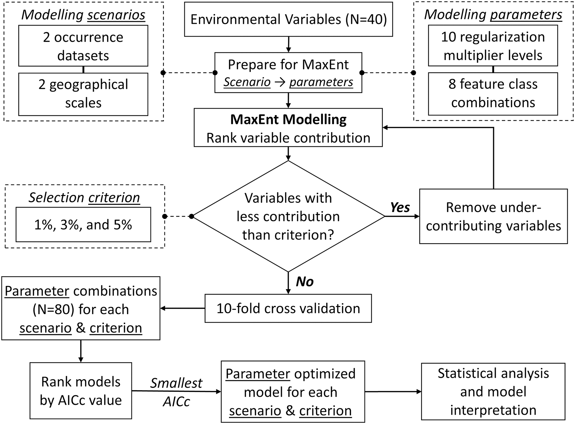
Results
eDNA detections of S. odoratus and eDNA-based occurrences
Our probe-based qPCR method was specific for S. odoratus detection in both laboratory and field, with no qPCR detections resulting from non-template controls nor DNA extracts from co-occurring turtles. The LOD of our eDNA assays was 10 copies per reaction, which extrapolates to 125 copies per litre of water (Fig. S3). In Lake Opinicon where S. odoratus is known to occur, we detected target eDNA signals for all 18 test samples (Fig. S3). For the eDNA field surveys, we found signals at 90 out of 145 sampled sites, resulting in 54 cells being marked as positive eDNA detections (i.e., some cells had more than one detection). Of these 54 cells, 47 did not have previous NHIC occurrences. The NHIC-only datasets for the Rideau and Southern Ontario modelling regions had 385 and 674 occurrences, respectively. With additional presences from eDNA surveys, the NHIC+eDNA datasets had 432 and 721 occurrences for the Rideau and Southern Ontario regions, respectively. Finally, at sampled sites where musk turtle eDNA was detected, the average ROR values from NHIC-only models were significantly higher than those where eDNA did not indicate musk turtle presence (Rideau: 1.90 × 10⁻⁴ vs. 4.35 × 10⁻⁵; Southern Ontario: 1.26 × 10⁻⁴ vs. 3.14 × 10⁻⁵. t tests, p ≪ 0.001. See Fig. S4).
How do eDNA occurrences alter niche models for musk turtles?
We optimized MaxEnt models balanced for model complexity and prediction accuracy (Table 1). For both modelling regions, we observed the same model parameters and similar variable response curves between models with or without eDNA occurrence data included (Table 1). Using a post hoc PCA, we categorized and retained the model variables based on their pair-wise correlations (Fig. S5, Table S3): temperatures (mean annual temperature and mean temperature of the warmest quarter), hydrological features (waterbody and total shoreline proportions), elevation (mean), and summer precipitation (warmest quarter). The addition of eDNA occurrences did not greatly alter our niche models in model variables included, predicted species presence, or inferred geographic distribution. For model variable composition in the Rideau region (Table 2), NHIC-only and NHIC+eDNA models had four of five variables in common differing only in ‘Grassland-shrub 5 km’ vs. ‘Mean temperature warmest quarter’. For model variable composition in the Southern Ontario region (Table 2), the two models shared the first eight variables, while the NHIC+eDNA model had one additional variable (Table 2), ‘Grassland-shrub 5 km’. For both regions, the two compared models predicted different S. odoratus distributions (i.e., RORNHIC+eDNA vs. RORNHIC-only), where models supplemented with eDNA detections predicted greater S. odoratus presence towards the north compared to the NHIC-only models (Fig. 3). Finally, based on the cumulative outputs of MaxEnt models, we were able to generalize the species range limits predicted by NHIC-only and NHIC+eDNA models (Fig. 4). Overall, presences predicted by NHIC+eDNA models shifted towards the Madawaska Highlands (an elevated area west of Algonquin Provincial Park), where the species has not been previously documented.
| Scenario | Parameters | Variables | Training AUC | Testing AUC | AUC difference | Criterion% |
|---|---|---|---|---|---|---|
| Rideau + NHIC-only |
LQ1.0 | 8 | 0.941 | 0.940 (0.014) | 0.002 | 1 |
| LQ1.0 | 5 | 0.935 | 0.934 (0.015) | 0.001 | 3 | |
| LQ1.0 | 4 | 0.933 | 0.932 (0.015) | 0.001 | 5 | |
| Rideau + NHIC+eDNA |
LQP4.5 | 13 | 0.934 | 0.931 (0.015) | 0.003 | 1 |
| LQ1.0 | 5 | 0.916 | 0.915 (0.019) | 0.001 | 3 | |
| LQ1.0 | 4 | 0.916 | 0.915 (0.019) | 0.001 | 5 | |
| S. Ontario + NHIC-only |
LQPT3.0 | 10 | 0.970 | 0.966 (0.008) | 0.004 | 1 |
| LQPT2.5 | 8 | 0.968 | 0.963 (0.008) | 0.005 | 3 | |
| LQPT3.0 | 7 | 0.967 | 0.963 (0.008) | 0.004 | 5 | |
| S. Ontario + NHIC+eDNA |
LQPT3.5 | 11 | 0.968 | 0.963 (0.007) | 0.004 | 1 |
| LQPT2.5 | 9 | 0.966 | 0.961 (0.008) | 0.005 | 3 | |
| LQPT2.5 | 7 | 0.963 | 0.959 (0.009) | 0.005 | 5 |
| Occurrence: NHIC-only | Occurrence: NHIC+eDNA | |||||
|---|---|---|---|---|---|---|
| Variable | Contr. | Response curve | Variable | Contr. | Response curve | |
| Rideau | Annual mean T. | 39.4 |  |
Annual mean T. | 34.7 |  |
| Total shoreline | 29.4 |  |
Total shoreline | 33.4 | 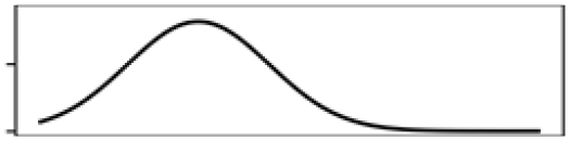 |
|
| Waterbody% | 16.9 | 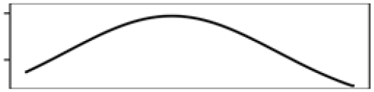 |
Waterbody% | 20.3 | 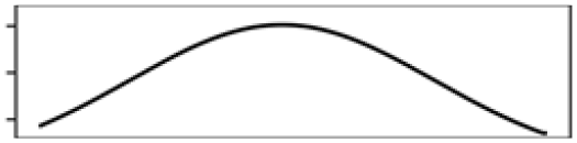 |
|
| Mean elevation | 10.5 | 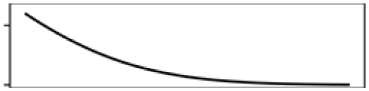 |
Mean elevation | 7.7 | 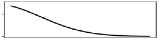 |
|
| Forest% 5 km | 3.9 | 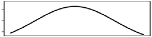 |
Mean T. warmest Q. | 3.8 | 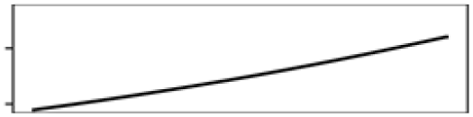 |
|
| Southern Ontario | Total shoreline | 23.0 |  |
Total shoreline | 21.0 | 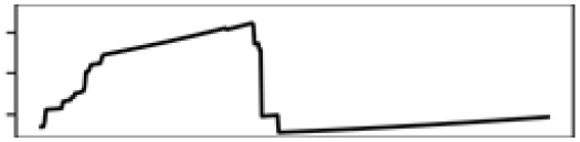 |
| Annual mean T. | 22.0 | 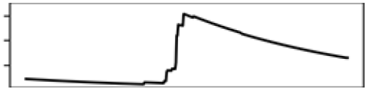 |
Mean T. warmest Q. | 20.1 |  |
|
| Mean elevation | 15.5 | 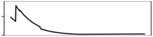 |
Mean elevation | 13.3 | 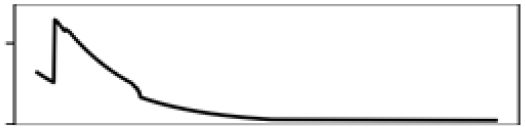 |
|
| Mean T. warmest Q. | 11.7 | 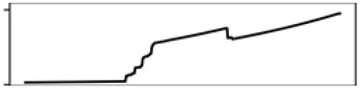 |
Annual mean T. | 12.2 | 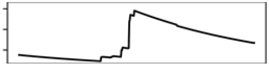 |
|
| Precp. warmest Q. | 9.9 | 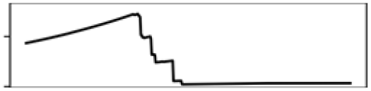 |
Precp. warmest Q. | 10.6 | 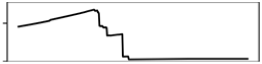 |
|
| Waterbody% | 8.2 | 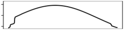 |
Waterbody% | 8.8 | 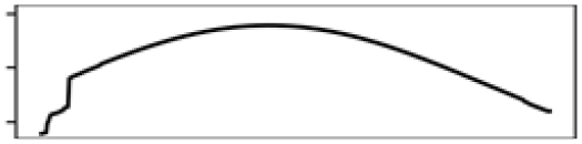 |
|
| Total shoreline 5 km | 6.3 | 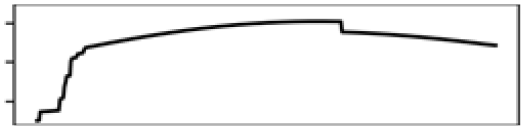 |
Total shoreline 5 km | 5.3 | 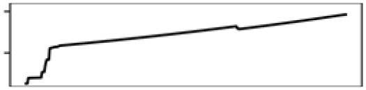 |
|
| Waterbody% 5 km | 3.4 | 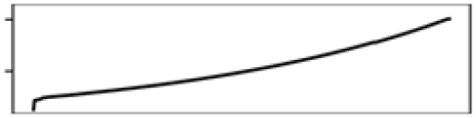 |
Waterbody% 5 km | 4.5 | 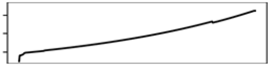 |
|
| Grass-shrub% 5 km | 4.2 | 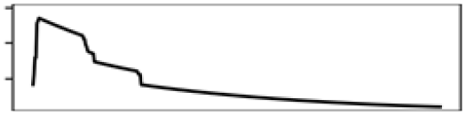 |
||||
Note:
Contr., contribution to model in percentage; M., month; Precp., precipitation; Q., quarter; T., temperature.
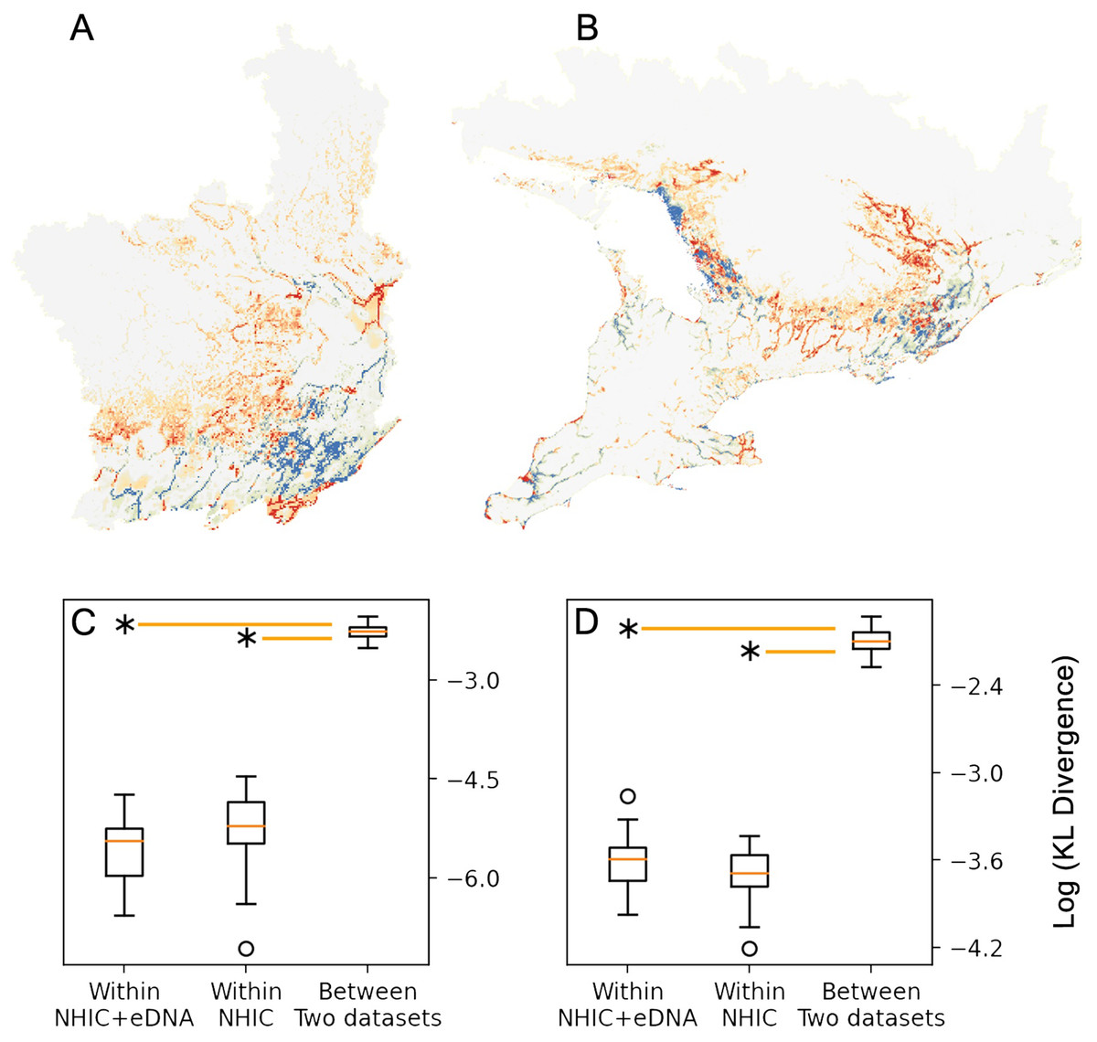
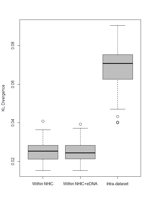
Figure 3: Comparison between MaxEnt relative occurrence rate (ROR) from NHIC-only and NHIC+eDNA models.
Comparison of ROR values derived from the NHIC-only and NHIC+eDNA models for the Rideau sampling region (A) and the larger, Southern Ontario sampling region (B). Warmer colors (red and orange) indicate areas where ROR values were higher for the NHIC+eDNA models than for the NHIC-only models while colder colours (blues) indicate the converse. (C and D) Comparisons of Kullback–Leibler divergence values (represented by DKL, log transformed on the Y-axes) for the two sampling regions for: (i) within NHIC+eDNA replicated models (N = 10); (ii) within NHIC-only replicated models (N = 10); (iii) between NHIC+eDNA and NHIC-only replicated models (N = 10, respectively). For both sampling regions, the median within-dataset DKL values for NHIC-only and NHIC-eDNA models are significant smaller than the median for between-dataset DKL values (Kruskal Wallis test, p ≪ 0.001 indicated by the asterisks) implying significant differences in ROR values.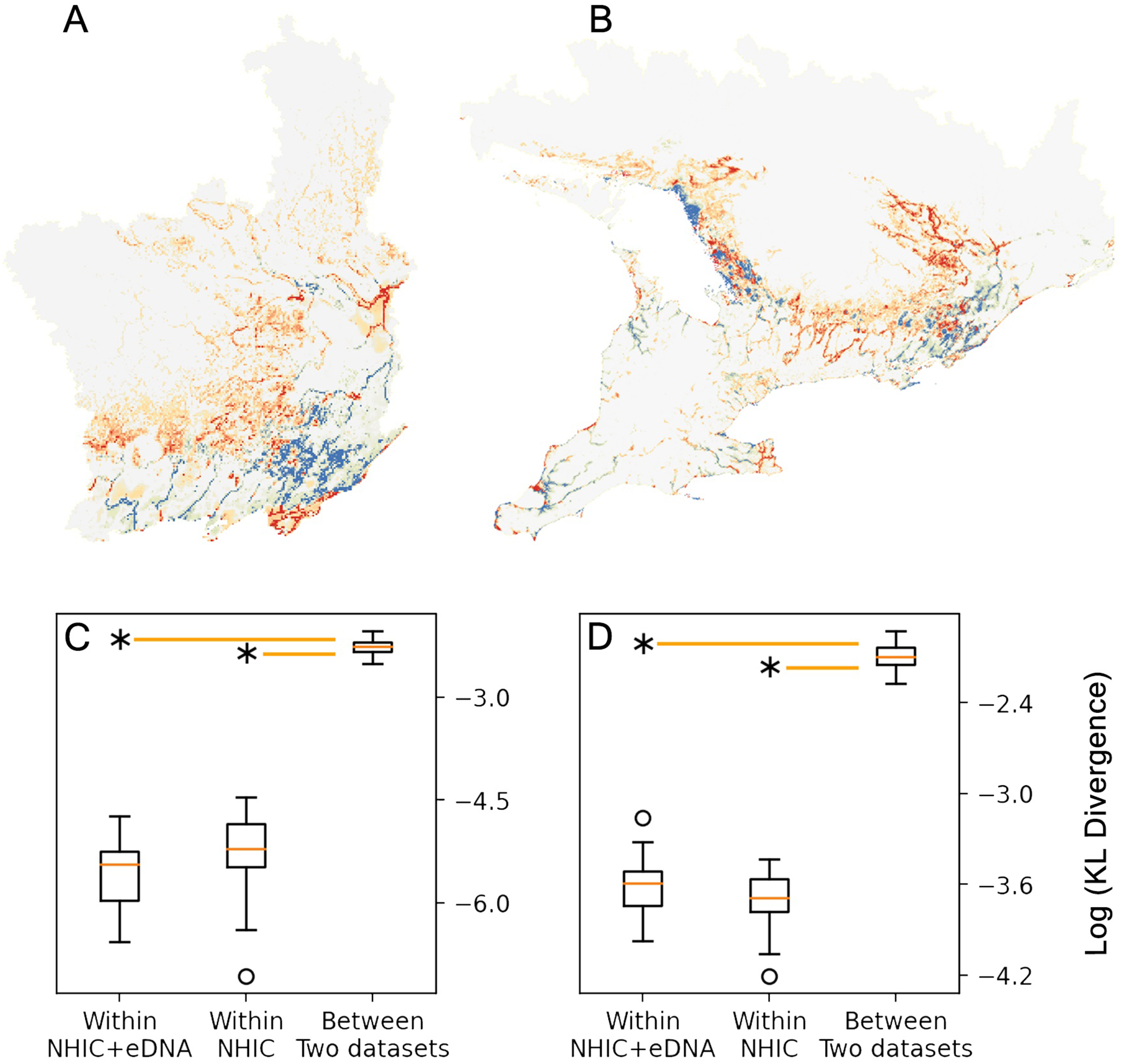
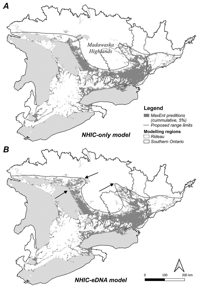
Figure 4: MaxEnt model cumulative output (5% false omission) in Southern Ontario region.
(A) NHIC-only model; (B) NHIC-eDNA model. Areas where the NHIC+eDNA model indicated Sternotherus odoratus presences while NHIC-only model did not are marked by arrows. Generalized northern range limit of S. odoratus distribution (dash line) are proposed.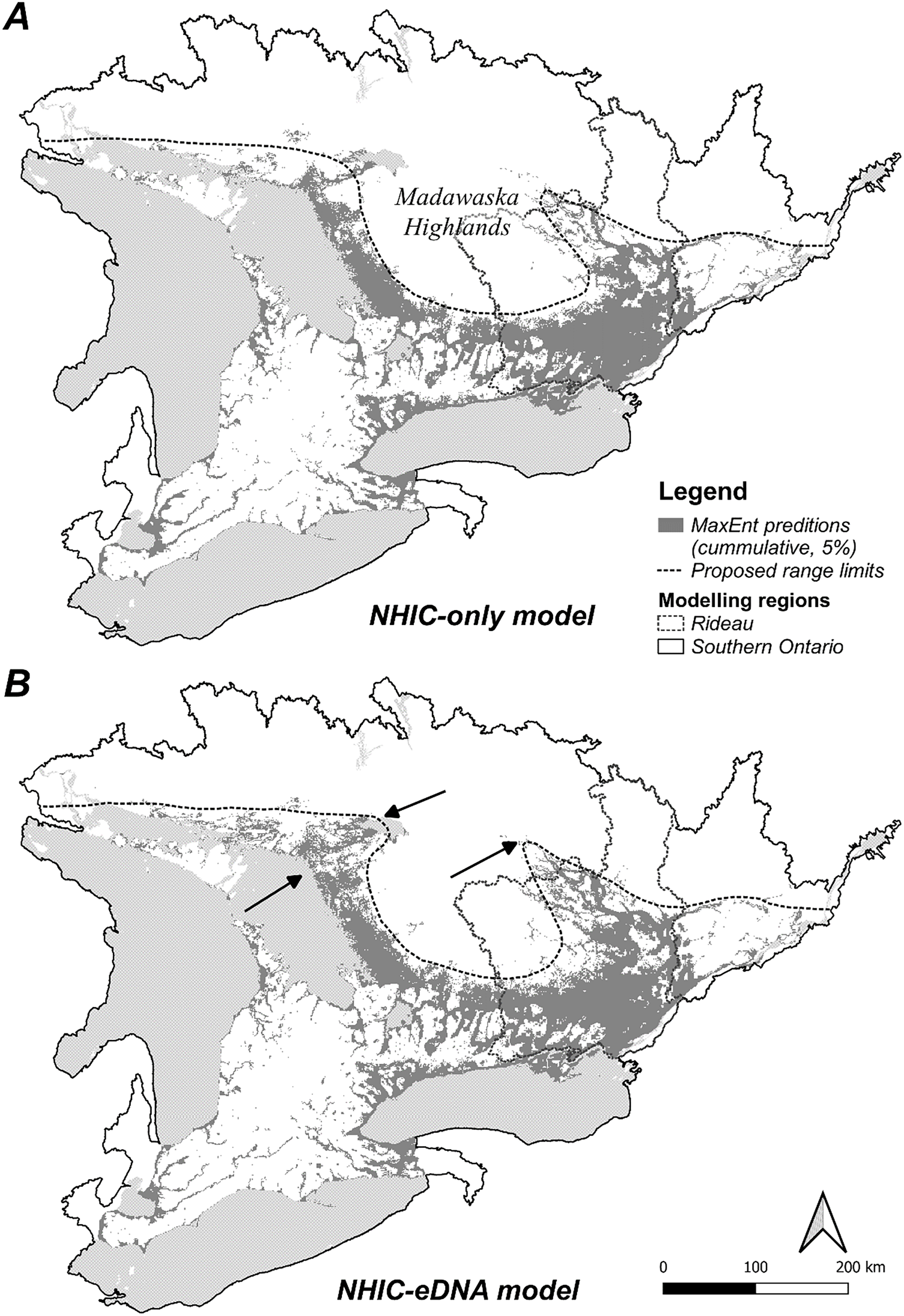
Discussion
Comprehensive surveys of organisms with cryptic habits or that are rare are critical to understand their ecology, to quantify factors that influence their distribution, and to guide conservation, but are often logistically challenging and expensive. We developed eDNA methods for the common musk turtle at its northern range limit in Southern Ontario, Canada. We show that eDNA reliably indicated the presence of musk turtles where they were known to occur. We also detected eDNA signals in areas where the species had not previously been recorded. Using combined citizen science observations and eDNA detections and a fully optimized MaxEnt framework, we modelled the northern distribution of the common musk turtle, finding the reported range to be incomplete. The addition of eDNA occurrences had only modest impact on our niche models and the explanatory variables retained. Overall, we were able to identify potential environmental factors that underlie the northern range limits of the study species and eDNA occurrences augmented our datasets and statistical power.
Relatively few eDNA studies have focused on reptiles compared to other vertebrates like fish or amphibians (Davy, Kidd & Wilson, 2015; but see Piaggio et al., 2014), although this is changing as eDNA applications become more widespread (Nordstrom et al., 2022). We designed and validated a probe-based qPCR assay to detect eDNA from S. odoratus. The LOD was approximately 10 copies per qPCR reaction, consistent with other eDNA assays for single species (Doi et al., 2015; Lam et al., 2020). The sensitivity assay indicated relatively high quantities of target eDNA molecules in sampled waterbodies. At locations where S. odoratus is present, it tends to occur in high densities. For example, at our field testing site, a mid-sized temperate, freshwater lake, the S. odoratus population has been estimated to exceed 6,000 individuals (Midwood et al., 2015). Sternotherus odoratus spends most of the time underwater with prolonged diving bouts (Heiss et al., 2010), which may lead to extra eDNA release relative to other species.
The geographical distribution of S. odoratus in Southern Ontario is probably underestimated. Our eDNA surveys enhanced our understanding of this species in multiple ways. First, we confirmed S. odoratus presence at locations that had high probability of S. odoratus presence in NHIC-only models. Our eDNA detections added to the explanatory value of our MaxEnt models, although the major environmental variables and response curve shapes were largely unchanged with additional eDNA detections. This was not unexpected as our eDNA surveys did not dramatically expand the range of S. odoratus, and thus we did not include new occurrences from areas that diverged dramatically in environmental attributes. For example, no eDNA detections were found at more northerly sites in Quebec where we tested for musk turtle presence beyond the species northern range limit (Fig. 1B); if we had affirmed presence at these sites, the models would have been altered more substantively as these sites exhibit attributes more typical of boreal environments. Model similarity (i.e., NHIC-only vs. NHIC+eDNA) was higher in the Southern Ontario region compared with models for the Rideau region, especially when we used less stringent model selection criteria (S4-5). This is probably because of a proportionately greater number of eDNA detections relative to all occurrences in the smaller vs. larger sampling regions (54 occurrences added to 385 vs. 674). Last, our combined NHIC+eDNA model predictions suggested that the range limit of S. odoratus might include parts of the Madawaska Highlands, an elevated, forested area east of Algonquin Provincial Park (Fig. 4B).
Species geographic boundaries change over time and understanding which factors constrain or promote range expansion is valuable, especially given the current rapid increase in atmospheric temperatures that is causing many organisms to shift to higher latitudes or elevations (Kelly & Goulden, 2008). For ectothermic animals, probability of extinction in response to climate change is generally higher than in endotherms (Aragón et al., 2010). Using traditional and eDNA surveys, we modelled the geographical distribution of S. odoratus at its current northern range limit finding it to be shaped mostly by thermal conditions, aquatic environmental characteristics, and elevation-related variables.
Thermal conditions are essential for reptile survival as reptiles lack physiological mechanisms to maintain body temperature (Bogert, 1949). We found that the predicted occurrence probability dropped quickly to zero in areas where mean temperature during the warmest quarter (i.e., summer) and annual mean temperatures are lower than 16 °C and 4 °C, respectively. Absence of positive eDNA signals along the Gatineau River well north of the species known range supported the assertion that temperature limits northern boundaries (Fig. 1B). Such a temperature threshold could exist for two reasons. While the thermal conditions during summer reflect the time when turtles forage and reproduce, low annual mean temperature also includes temperatures from winter which if prolonged would limit the ability of the species to persist. Our predicted S. odoratus presence was greater as temperatures increased, peaking at an annual mean temperature of 6 °C and then declining modestly thereafter (Table 2, Figs. S6 and S7). The decline in predicted occurrence is possibly an artefact of local extirpation of the turtle in the southern part of our modelling area with higher temperatures, where many wetlands were lost because of agriculture and urbanization (Ducks Unlimited Canada, 2010).
The ecology together with the physical characteristics of aquatic habitats of S. odoratus towards its northern range limit probably constrain its distribution. During summer, shallow aquatic environments provide essential foraging grounds and warm ambient temperatures for basking (Ernst & Lovich, 2009). During winter in Southern Ontario, however, most waterbodies freeze, sometimes for up to 6 months, and S. odoratus retreats to brumate in deeper waters. Because S. odoratus is anoxia intolerant (Ultsch, 1988), underwater overwintering sites must provide sufficient dissolved oxygen for their physiological needs. MaxEnt models from both modelling regions for both datasets suggested that S. odoratus is most likely to be present in areas with approximately 50% water surface and 10% shoreline (Figs. S6 and S7). An optimal habitat then is a mid-sized waterbody that provides for summer foraging and basking and overwintering. In contrast, the turtle is unlikely to be present in a large, deep lake with limited areas to forage, or a shallow lake with nowhere to overwinter. Our MaxEnt models support the long-held assertion that range limits of turtles at northern latitudes could be constrained by availability of overwintering habitat (Ultsch, 2006), where freshwater turtles typically overwinter underwater beneath the ice. Surveying winter distributions of temperate turtles by traditional methods (e.g., under-ice snorkelling) can be logistically challenging and eDNA assays have been tested under ice in focal waterbodies to infer their distributions (Feng, Bulté & Lougheed, 2020; Tarof et al., 2021).
Our models with and without eDNA predicted that the presence of S. odoratus drops rapidly with increasing mean elevation and that it is absent above 400 m (Figs. S6 and S7), aligning with the fact that its documented distribution has a prominent gap in the Madawaska Highlands (mean elevation >400 m). This species is more likely to disperse via rivers and streams than overland (Ernst & Lovich, 2009). Migration from low to high altitudes might be somewhat physically limited. More likely is that higher elevations have longer winters with more extended periods of ice cover and thus would result in shorter active seasons for turtles. However, our models did not select annual mean snow days as a significant variable, possibly because this predictor was created using large scale remote sensing data for the entire Northern Hemisphere (1 km2 resolution. source: NOAA. https://nsidc.org/data/g02156) and thus does not have sufficient resolution. Precipitation of the warmest quarter (i.e., July to September) showed similar thresholding behavior, as S. odoratus was predicted to be absent in regions with over 270 mm in summer precipitation. Though studies of the effects of summer precipitation on fitness and survivorship of freshwater turtles are lacking, it is evident that both summer precipitation and elevation have negative effects on lake summer surface temperatures (Minns et al., 2018). During the summer months when conditions are suitable for growth and reproduction, excessive rainfall may lead to colder surface water that hinders thermoregulation and overall activity.
Finally, the current northern distribution of S. odoratus has been shaped by human activities in Southern Ontario, the most densely populated area in Canada. In southwestern Ontario, over 85% of the original wetlands have been converted for urban and agricultural use since the onset of European settlement (Ducks Unlimited Canada, 2010). This area undoubtedly previously housed S. odoratus and other turtle species, and human activities have profoundly affected their distributions. However, our niche modelling framework implied that no farmland and urban landscape variable made significant contributions to the final models. It is possible that the distribution of musk turtles has not yet reached equilibrium in these highly disturbed areas, implying that habitat loss due to land conversion is a cause of local extirpation of S. odoratus rather than a driver of the turtle’s northern distribution limits.
Conclusions
We developed a robust, sensitive, and species-specific eDNA field survey protocol for the common musk turtle. Ours is among the few eDNA studies dedicated to niche modelling of an aquatic reptile species. eDNA allowed us to test for the turtle’s extra-limital occurrences, and augmented our citizen science dataset, and expanded the range into areas where it has not been documented. eDNA surveys in aquatic environments can easily be reproduced and expanded to larger geographical scales, providing valuable information on contemporary distributions and guiding conservation management efforts. In an era of rapid climate change, eDNA affords an effective way to monitor shifting distributions and detect range expansions of aquatic species at the very earliest stages of range expansion. As eDNA survey methods continue to improve, more niche modelling studies that incorporate eDNA survey data will undoubtedly reveal improved distribution maps and novel insights on the factors that shape geographic range limits across species.
Supplemental Information
Environmental DNA extraction protocol.
Protocol for chloroform-based DNA extraction method modified from (Turner et al. 2014) for eDNA samples.
Standard curve construction for qPCR assays.
Methods for constructing standard curves for qPCR assays including creating plasmid with amplicon insert of focal marker.
Parameter optimization and analyses for MaxEnt modelling.
Detailed steps for parameter optimization for MaxEnt model construction including consideration of different feature classes, regulization multiplier, backward stepwise selection, and cross-validation.
Optimized MaxEnt models from 1% and 5% selection criterion.
Presented in the main text are results from optimized MaxEnt models using a 3% selection criterion. Results in this supplementary material show results using different cut-offs: 1% and 5%.
Seven supplementary tables relating to methods and results from MaxEnt modeling.
Tables relating to eDNA primer development (Table S1), environmental layers used in modeling (Table S2), and parameter optimization and model choice (Tables S3 through S7).
Annual trend of observational records of S. odoratus in NHIC dataset.
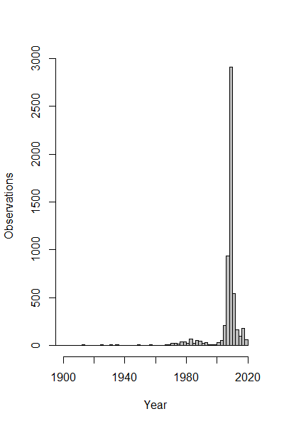
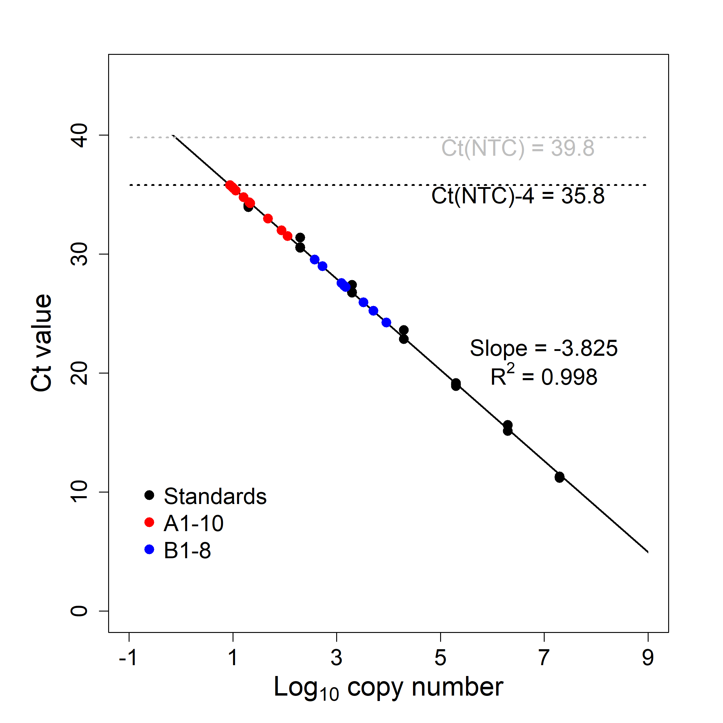
eDNA sample sites during summer 2016 in Lake Opinicon (Frontenac, Ontario, Canada) at two locations (NA = 10, NB = 8) where S. odoratus are known to occur.
Testing results for qPCR essay for eDNA detection in Lake Opinicon for Sternotherus odoratus.
Black dots and line represent the seven-point standard curve. Template copy number per reaction of the initial standard was 2×10⁷ and the consequent standards followed a 10-fold serial dilution. Results of eDNA samples taken from two sites (A and B) of known S. odoratus activity in the lake are also plotted (NA = 10, NB = 8). A horizontal dashed line shows the value of Ct of non-template controls minus four (Ct-NTC - 4), which was used to determine the lower detection limit of the qPCR assay (10 copies per reaction).
Predicted relative occurrence rate (ROR) from NHIC-only MaxEnt models at eDNA survey sites.
Grey and white bars show ROR values at survey sites of S. odoratus eDNA detections (N = 90) and non-detections (N = 45), with the significance of difference showed by asterisks (t test, ***: p ≪ 0.001).
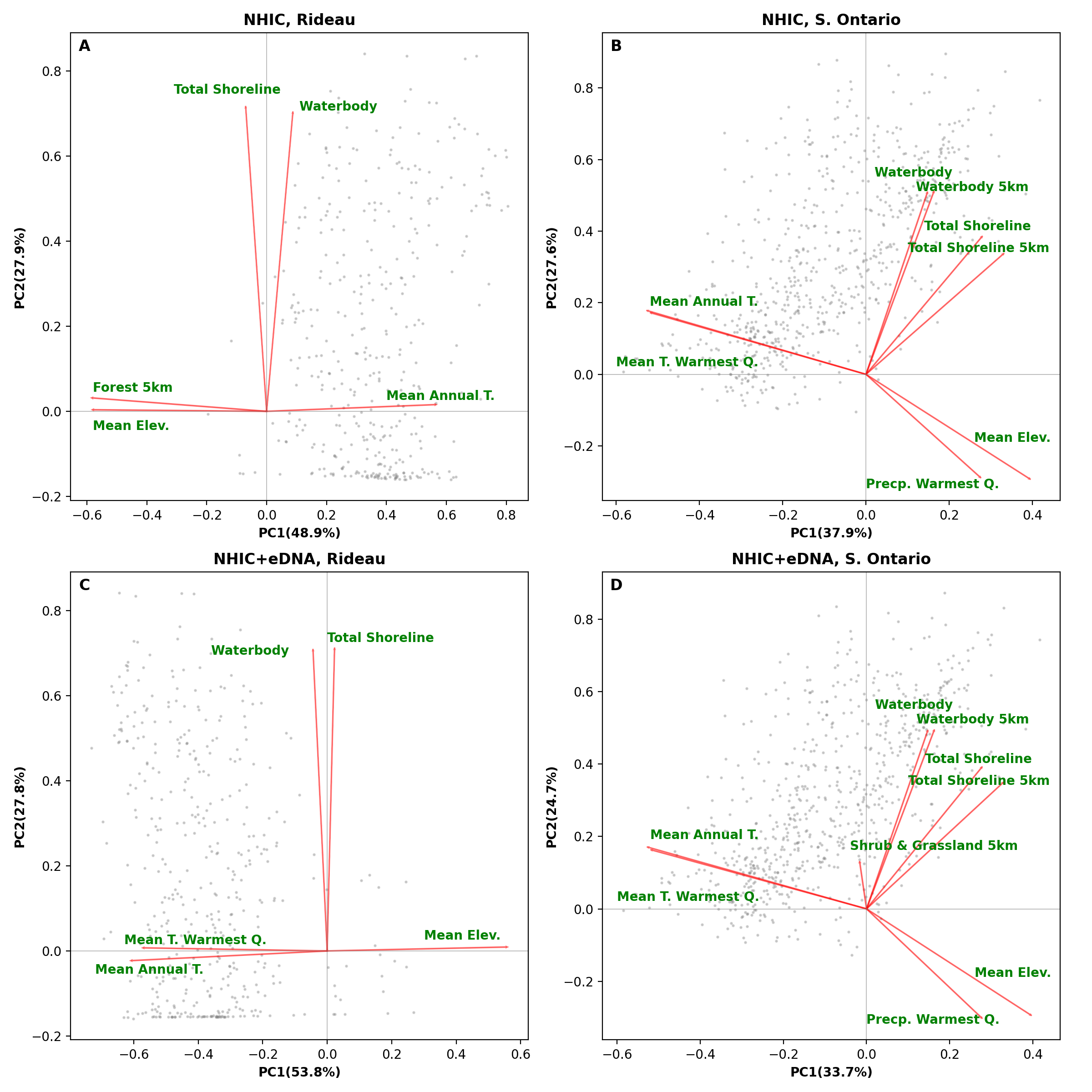
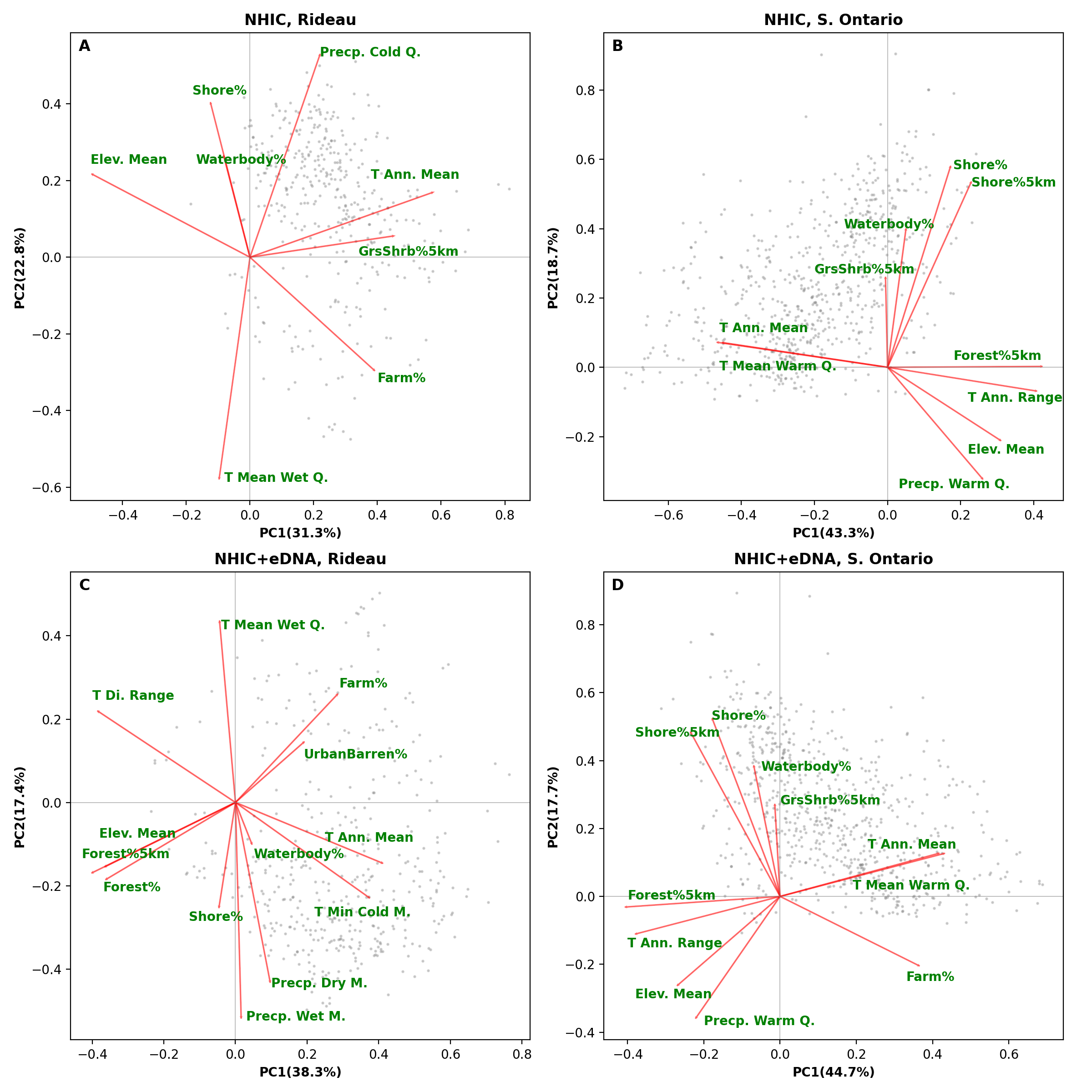
Biplots from a principal component analysis (PCA) of environment variables from the optimized MaxEnt models.
The top panel (A-B) shows the results of PCA on models based on NHIC-only dataset and the bottom panel (C-D) shows PCA results from models based on NHIC+eDNA dataset. The left panels (A and C) show models at the scale of Rideau region and the right panels (B and D) show models at the scale of Southern Ontario. Grey dots in the figure indicate scores of the occurrences used in the model. Abbreviations: Elev. – elevation; Precp. – precipitation; Q. – quarter; T. – temperature.
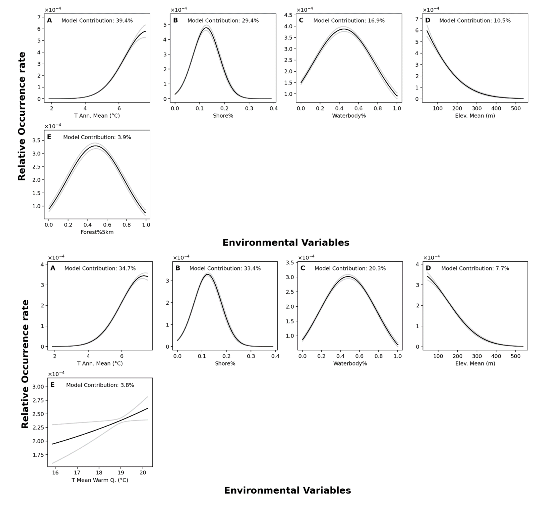
Response curves from MaxEnt models in Rideau region.
Top panel: NHIC-only dataset. Bottom panel: NHIC+eDNA dataset. Model contribution of each variable is shown. This figure shows models optimized under 3% backward selection criterion.
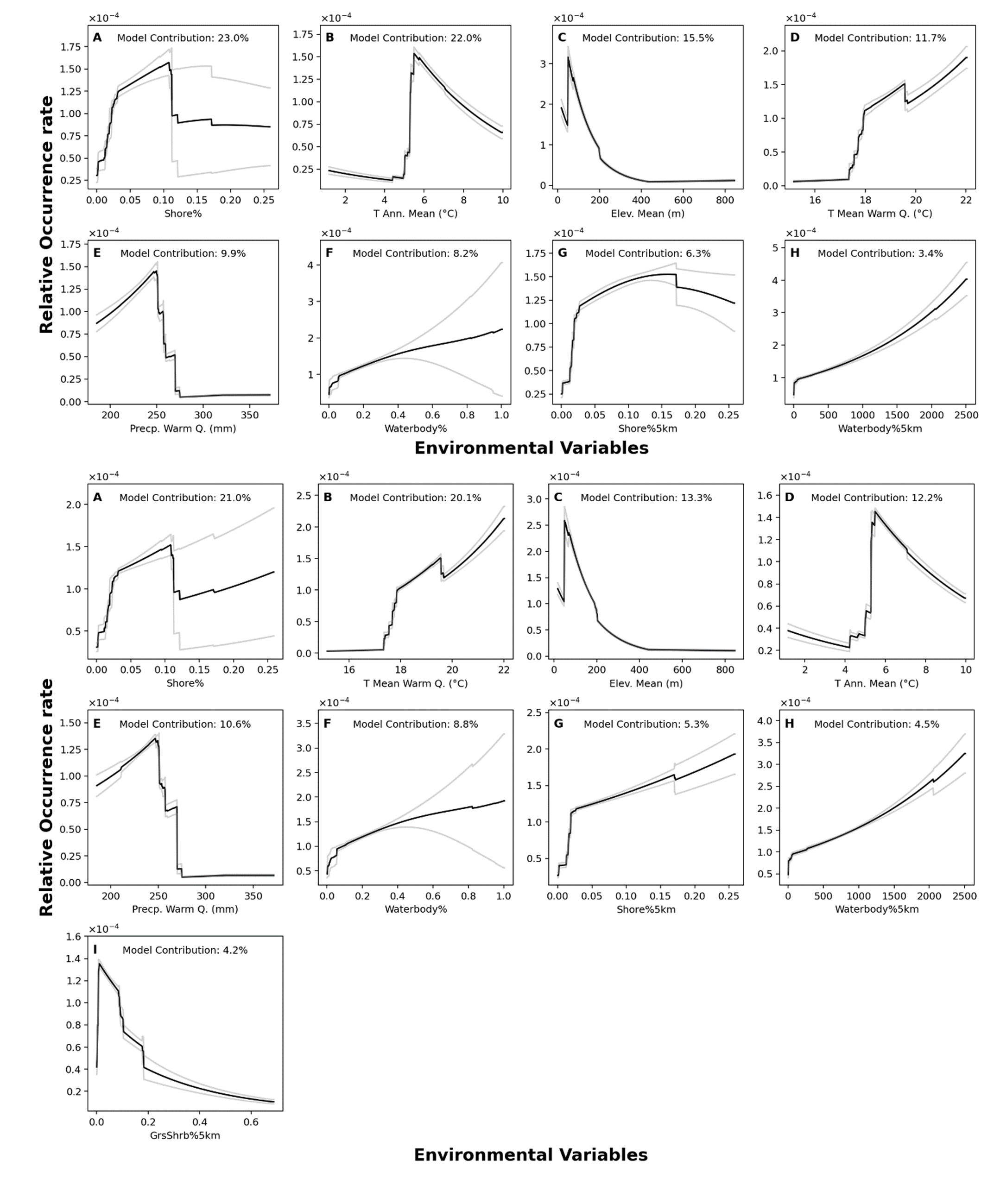
Response curves from MaxEnt models in Southern Ontario region.
Top panel: NHIC-only dataset. Bottom panel: NHIC+eDNA. Model contribution of each variable is shown. This figure shows models optimized under 3% backward selection criterion.
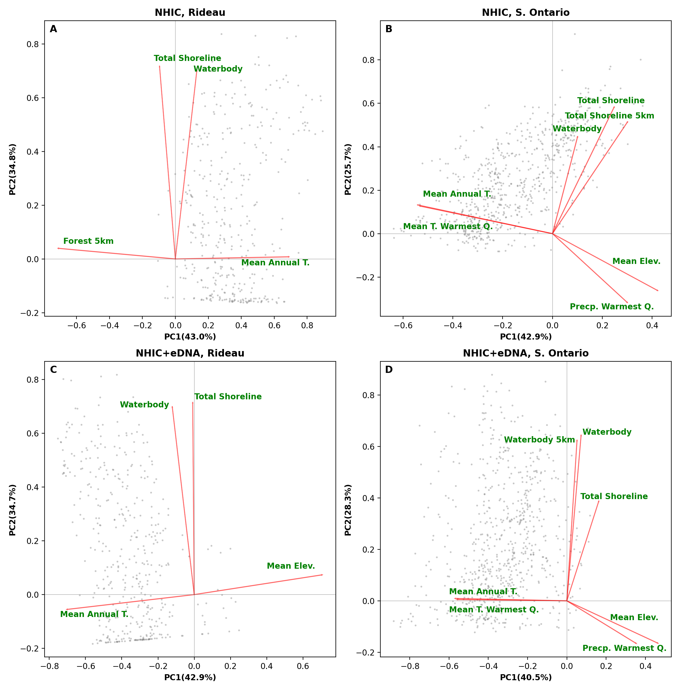
Biplots from a principal component analysis (PCA) of environment variables from the optimized MaxEnt models rom 1% backward selection criterion.
The top panel (A-B) shows the results of PCA on models based on NHIC-only dataset and the bottom panel (C-D) shows PCA results from models based on NHIC-eDNA dataset. The left panels (A and C) show models at the scale of Rideau region and the right panels (B and D) show models at the scale of Southern Ontario. Grey dots in the figure indicate scores of the occurrences used in the model. Abbreviations: Elev. – elevation; Precp. – precipitation; Q. – quarter; T. – temperature.
Biplots from a principal component analysis (PCA) of environment variables from the optimized MaxEnt models from 5% backward selection criterion.
The top panel (A-B) shows the results of PCA on models based on NHIC-only dataset and the bottom panel (C-D) shows PCA results from models based on NHIC-eDNA dataset. The left panels (A and C) show models at the scale of Rideau region and the right panels (B and D) show models at the scale of Southern Ontario. Grey dots in the figure indicate scores of the occurrences used in the model. Abbreviations: Elev. – elevation; Precp. – precipitation; Q. – quarter; T. – temperature.