Good Practices for Species Distribution Modeling of Deep-Sea Corals and Sponges for Resource Management: Data Collection, Analysis, Validation, and Communication

Introduction

Deep-sea corals and sponges (DSCS) are among the longest-living sessile marine organisms and are important biogenic components of habitat in many marine ecosystems (Roberts et al., 2009; Buhl-Mortensen et al., 2010; Hogg et al., 2010; Rossi et al., 2017). They are a diverse group of habitat-forming invertebrates spanning two phyla and exhibiting numerous growth habits; some species reaching meters in height and others forming large reefs (Roberts et al., 2009; Maldonado et al., 2017). Like their tropical counterparts, DSCS create hotspots of diversity by providing structure and refuge for many invertebrates and fishes, especially when forming dense aggregations (Stone, 2006, 2014; Buhl-Mortensen et al., 2010; Baillon et al., 2012). DSCS are suspension feeders, making them important contributors to carbon and nutrient cycling in the deep ocean (Cathalot et al., 2015; Maldonado et al., 2017), but are fragile and slow-growing, making them vulnerable to human impacts like fishing, deep-sea mining, offshore oil and gas development, etc.

Due to their vulnerability and the many ecosystem functions they provide, DSCS have received increasing attention from conservationists and resource managers worldwide. Internationally, they have been identified as key indicator taxa for vulnerable marine ecosystems [FAO (Food and Agriculture Organization of the United Nations), 2009] and ecologically or biologically significant marine areas [Convention on Biological Diversity (CBD), 2010]. In the United States (U.S.), several laws provide the authority to regulate offshore activities (e.g., fishing, energy development, and leasing) that might damage environmentally sensitive seafloor habitats. For example, in 1984 the U.S. established the Oculina Banks Habitat Area of Particular Concern off Florida, the first area specifically designed to protect deepwater coral reefs from fishing impacts. Since 2005, deep-sea coral conservation efforts have accelerated across the U.S. Exclusive Economic Zone (EEZ), with a focus on protecting seafloor habitats from impacts of fishing gear (Figure 1; Hourigan et al., 2017). These area-based gear restrictions included large precautionary closures in deep water designed to freeze the footprint of bottom trawling (Figure 1), the type of fishing usually considered the most substantial threat to DSCS (Clark et al., 2016a; Rooper et al., 2017b). This approach has prevented the expansion of the most damaging fishing into deeper waters (Hourigan, 2014), but also means that further conservation gains will require more targeted information and management within the footprint of existing fisheries. The National Oceanic and Atmospheric Administration's (NOAA) Deep Sea Coral Research and Technology Program (DSCRTP; https://deepseacoraldata.noaa.gov/), in partnership with other NOAA offices, federal agencies, and academic and stakeholder groups funds and coordinates research and supports the development of management measures to protect DSCS.

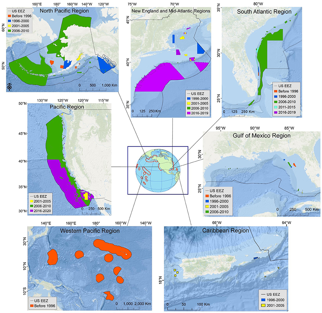
Figure 1. Restrictions on bottom-trawling, usually considered the most substantial threat to deep-sea coral and sponge habitat, in the U.S. exclusive economic zone (EEZ) as of January 2020. Protections are illustrated by year of implementation and grouped as taking effect before 1996 (the year essential fish habitat was introduced; red polygons), or between 1996–2000 (dark blue), 2001–2005 (yellow), 2006–2010 (green), 2011–2015 (light blue), or 2016–2019 (purple). The Pacific Region map legend includes 2020 because the Pacific Fishery Management Council approved trawl restrictions in 2018 that were enacted on 1 January 2020. Note the different geographic scales used for each region. The New England and Gulf of Mexico Fishery Management Councils approved additional protections in 2018 that were yet to be enacted by the time of publication, so are not shown here.

Species distribution modeling (SDM) is a technique for quantifying species-environment relationships and applying those relationships to predict and map the abundance or habitat of species of interest (e.g., Guisan et al., 2017). SDMs use biological and environmental data as input and produce distribution maps at spatial scales relevant to management. The majority of existing DSCS SDMs are “presence-only” models, often applications of maximum entropy (MaxEnt) and ecological niche factor analysis (ENFA) (Figure 2; Vierod et al., 2014; Guinotte et al., 2017). These models make use of the most commonly available type of biological data for DSCS: locations of observed occurrences of individual taxa. The maps produced from presence-only models indicate where suitable habitat is predicted to be more or less likely. These maps have been used to guide targeted field surveys in underexplored areas (Georgian et al., 2014), to inform management decisions made by regional fisheries management organizations (Vierod et al., 2014; Georgian et al., 2019) and U.S. regional fishery management councils (Kinlan et al., 2020), to examine potential environmental covariates of DSCS habitat (Etnoyer et al., 2018), and to provide information to the U.S. Bureau of Ocean Energy Management for its environmental compliance and leasing decisions (Bauer et al., 2016). However, presence-only models have limitations (e.g., lack of data on sampling effort) that reduce their usefulness for effective management of DSCS. Alternative SDM techniques exist that can overcome these limitations and have been applied to DSCS (Figure 2), but these techniques generally require additional types of biological data (e.g., absence or density data).

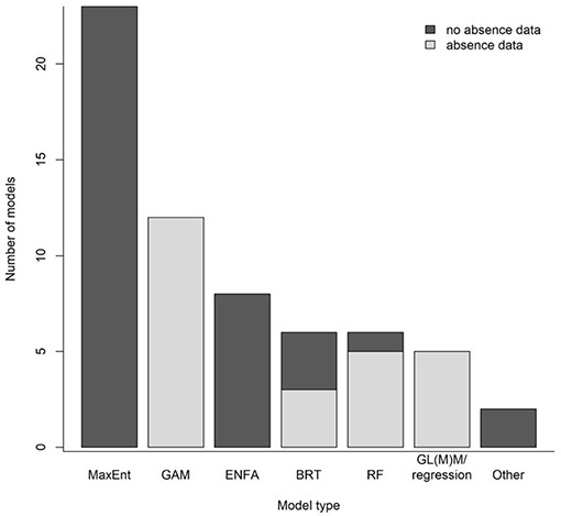
Figure 2. Types of deep-sea coral and sponge species distribution models in 42 studies (journal articles, government technical reports, and book chapters) published between 2005 and 2019 (Supplementary Material). Common model types were maximum entropy (MaxEnt), generalized additive model (GAM), environmental niche factor analysis (ENFA), boosted regression tree (BRT), random forest (RF), and generalized linear (mixed) model (GL(M)M). Note that some studies employed more than one model type, so the total number of models is greater than the number of studies.

To better manage human activities impacting DSCS, managers and analysts would benefit from an improved understanding of current data limitations, preferred SDM approaches, and future data needs. In this paper, we describe good practices for the data and methods needed to inform SDMs of DSCS distributions for management purposes. We also present three case studies from the Pacific Ocean, including two from U.S. waters, that highlight some of the challenges associated with these data and methods. Our good practices are not meant to be a “one size fits all” solution. Individual scientific and management needs, data availability, intended application, funding availability, and field logistical constraints may require individualized approaches to data collection and modeling. Our interest and objective is to provide “good practices” to help guide data collection and analysis by the DSCS research and management community.

Good Practices

Our good practices are first presented for biological and environmental data included in DSCS SDMs followed by analytical methods and then management applications. Case studies that illustrate our good practices (Table 1) are presented in the next section.

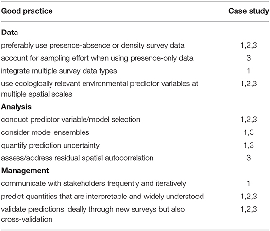
Table 1. Key good practices and illustrative case studies.

Data

Biological Data

Because the logistical and technical complexities and expense of operating at deep depths are limiting factors for collecting observations of deep-sea biota, DSCS SDMs built at global and regional scales typically include biological data from a range of sources (Vierod et al., 2014; Anderson et al., 2016a; Rooper et al., 2019). Many of the earlier DSCS SDMs relied on presence data compiled from historical records of DSCS observations, including from existing databases, museum collections, and cruise reports (Davies and Guinotte, 2011; Vierod et al., 2014). More modern biological data available to DSCS SDMs have been obtained at finer scales from georeferenced videos or photos collected during seafloor surveys (e.g., manned submersibles, autonomous underwater vehicles, and remotely operated vehicles) or from fisheries trawl surveys (Vierod et al., 2014). Many of these data have been reported only as DSCS presences, sometimes because of concerns over the ability to confirm the complete absence of a species in an observation (Vierod et al., 2014). However, because of the limitations of SDMs built with presence-only data (described in Section Analysis), we recommend that DSCS biological data from fine-scale surveys be recorded to quantify presence-absence, abundance, biomass, or density (abundance or biomass per unit area) (Case Studies 1–3) with a measure of effort for each sampling unit (e.g., area surveyed). From a practical standpoint, resource managers are most interested in identifying areas of potential high density or diversity of vulnerable DSCS rather than simply presence. Both density and size of DSCS are likely ecologically important factors for habitat use by other species (e.g., Case Study 1 and also Du Preez and Tunnicliffe, 2011). When the only data available are presence, analysts should attempt to recover or infer the distribution of sampling effort and the locations of absences if feasible by re-analysis of existing data, recognizing that this will increase the time required for analysis. For example, absence “observations” along a transect can sometimes be recovered from existing data recordings, or can be inferred from locations where other species were recorded as present during the same surveys (e.g., Case Study 3 and also Isaac et al., 2014).

Future sampling programs should record biological data at the highest taxonomic resolution possible. Models developed using data with low taxonomic resolution may mix species with very different life-histories and environmental requirements, resulting in overly broad predicted distributions and potentially increased model uncertainty. Models of functional groups or otherwise reduced taxonomic resolution may be sufficient to address some management applications, but in some cases models may be needed for specific taxa like species of concern (e.g., endangered species). We recognize that the identification of DSCS species, especially from images alone, can be difficult and their taxonomy is an active area of research, so these issues can be challenging to the development of models with high taxonomic resolution.

Most DSCS distribution modeling currently relies on existing data collected for other purposes. Given the increasing use of SDMs for management, future biological data collection should be designed to inform improved models including increased attention to statistically-robust survey design (Williams and Brown, 2019), along with measures of abundance, density, size, and survey effort. A centralized DSCS data repository, akin to the DSCRTP data portal (https://deepseacoraldata.noaa.gov/), hosting DSCS data collected and analyzed with these suggested data standards would facilitate SDMs to inform management.

Environmental Data

We focus on SDMs that integrate DSCS biological data with environmental data as covariates. Informative covariates often include measures of depth, seafloor terrain (e.g., slope, aspect, curvature, bathymetric position, ruggedness), and substrate properties (e.g., sediment composition), usually derived from remotely sensed acoustic bathymetry and backscatter data or geological samples (Wilson et al., 2007; Brown et al., 2011; Vierod et al., 2014; Rooper et al., 2016; Guinotte et al., 2017). Oceanographic properties (e.g., water temperature, chemistry, and current speed and direction) derived from field samples, remotely sensed data, and ocean models can also be informative covariates (Davies and Guinotte, 2011).

It is important to consider whether environmental covariates are available at spatial scales and resolutions that are relevant to management needs and to the ecological patterns and processes of interest (Davies and Guinotte, 2011). Mismatches in spatial scale and resolution between environmental covariates and management needs risk a loss of information necessary for effective management. Mismatches in spatial scale and resolution between environmental covariates and important ecological processes risk the failure to detect important relationships and can compromise the accuracy of predicted species distributions. The relevant ecological spatial scale may vary by DSCS species or functional group, so we suggest analysts consider environmental covariates at multiple spatial scales, but first use a hypothesis-driven approach to decide which scales may be most appropriate to include.

Spatial resolution and accuracy are important considerations in determining which bathymetry data to use in DSCS SDMs. Earlier DSCS SDMs built at global and basin scales typically included depth and seafloor terrain covariates derived from coarse bathymetry data from satellite altimetry or from compilations of hydrographic data. However, at coarse resolution these covariates may not resolve fine-scale seafloor features that provide habitat for DSCS. We suggest that DSCS SDMs include depth and seafloor terrain covariates derived from multibeam acoustic bathymetry data (that are collected at International Hydrographic Organization standards when possible), followed by regional (e.g., Zimmermann et al., 2013) and basin-scale [e.g., GEBCO (General Bathymetric Chart of the Oceans) Compilation Group, 2019] bathymetry compilations with rigorous data assembly methods, followed by bathymetric models and opportunistic measurements (e.g., Olex software¹; Jakobsson et al., 2012). We suggest researchers evaluate whether the spatial resolution of the bathymetry data and consequently derived seafloor terrain metrics will capture habitat processes that are ecologically important to DSCS. Certain terrain metrics, such as ruggedness measures, should not be derived from compilations of bathymetry data sets of varied quality and resolution.

High resolution multibeam acoustic seafloor scattering strength (backscatter) can be applied directly as a covariate or to derive measures of angular response, and seafloor properties such as hardness, ruggedness, and substrate composition (e.g., Brown et al., 2011). Backscatter data have been applied to distinguish (Weber et al., 2013) and model (Pirtle et al., 2015) the spatial extent of trawlable and untrawlable seafloor types where DSCS occur and in DSCS SDMs (Dolan et al., 2008; Buhl-Mortensen et al., 2012; Rowden et al., 2017). Backscatter is a relative measure, and compilations of backscatter from multiple surveys should generally only be used in SDMs when the acoustic surveys have collected backscatter using frequencies that do not differ by more than one octave (Hughes Clarke, 2015), and when the surveys have been relatively calibrated across years, platforms, and sensors (Lurton and Lamarche, 2015).

Oceanographic data include biological, chemical, and physical oceanographic properties, such as surface chlorophyll concentration, oxygen and aragonite saturation, temperature, salinity, current speed and direction, and turbidity. Oceanographic data collected during surveys or modeled based on survey data [e.g., Regional Ocean Modeling Systems (ROMS); (Hermann et al., 2016; Fiechter et al., 2018)] are generally of much coarser resolution than seafloor mapping data (km vs. m) and sometimes require interpolation to the spatial extent of management areas (e.g., Brown et al., 2011). These oceanographic covariates have been useful to model and predict DSCS distribution and habitat (Georgian et al., 2014, 2019; Rooper et al., 2014, 2017a; Bargain et al., 2018).

We suggest that analysts fit multiple SDMs with different environmental covariates at multiple scales to identify the best performing model (e.g., Wilson et al., 2007; Pirtle et al., 2019; Weijerman et al., 2019; Dove et al., 2020), and only retain the important environmental covariates at the appropriate scales in SDMs (Case Studies 1-3). From an ecological modeling perspective, it is also prudent to consider only those covariates that have realistic direct or indirect linkages to biological and ecological processes that would be expected to influence DSCS distribution (Case Studies 1-3). It is important that researchers factor in the potentially extensive time required for literature review, synthesis, and expert involvement for covariate development during the planning phase of a modeling project.

Analysis

Presence-Only Models

Presence-only models, like MaxEnt and ENFA, have been the most commonly employed SDM techniques for DSCS (Figure 2; Vierod et al., 2014; Guinotte et al., 2017). These methods have proven useful for some applications such as guiding surveys for exploration (Georgian et al., 2014), contributing to the development of conservation areas (Kinlan et al., 2020), and providing a foundation for subsequent higher-resolution modeling with alternative methods (Case Study 3). Indeed, presence-only models are the only option when only presence data are available. However, presence-only models have several disadvantages that are not conducive to effective management of DSCS. The major limitation of presence-only models is that sampling effort and resource density are confounded when the former is not appropriately represented in the model (Peel et al., 2019). Presence-only models can mistakenly identify well-sampled areas with many presence observations as areas with greater densities in contrast with less-sampled areas with fewer presence observations, even if densities are similar between areas (Fithian et al., 2015). That being said, presence-only models can accommodate and correct for independent information about the distribution of sampling effort when it is available (e.g., MaxEnt; Elith et al., 2011), and several approaches have been used to attempt to account for sampling effort when direct information is not available (Merow et al., 2016; El-Gabbas and Dormann, 2018). Another limiting issue with presence-only models is that they do not appropriately account for the effect of sampling effort on estimates of model uncertainty (Renner et al., 2015). Finally, it is not clear how to generalize presence-only models. Predictions from these models are usually in relative terms and the predicted quantities (e.g., relative habitat suitability) can be difficult to interpret and validate. As a result, inference across species and models is challenging, inhibiting the use of presence-only models for understanding community structure and DSCS-fish associations.

Preferred Modeling Frameworks

Given the limitations and challenges associated with presence-only models, we recommend using alternative modeling frameworks when possible (Case Studies 1-3). When data types other than presence are available (e.g., presence-absence, count, biomass), analysts should preferentially employ these data types to develop DSCS SDMs that produce predictions that are straightforward to interpret and validate (e.g., probability of occurrence for presence-absence data). Use of absence, count, or biomass data will naturally account for the distribution of sampling effort in the model, by including data from areas where taxa were detected and where they were not. It is also important to account for the amount of sampling effort (e.g., area viewed, trawl swept area) represented by each data replicate in a model, either by expressing the modeled response data (e.g., biomass) per unit of effort, or, in the case of presence-absence and count models, by including an effort “offset” in the model. Modeling approaches such as generalized linear models (GLMs), generalized additive models (GAMs), boosted regression trees (BRTs), and random forest models (RFs) accommodate these data types and model features.

Integration of Multiple Datasets and Types

In some cases it may be appropriate to combine multiple biological datasets. A common issue with DSCS sampling data is that the spatial footprint of an individual sampling program often does not cover the entire geographic area of interest to management or the geographic range of the species. A solution to this issue is to fit SDMs to data collected by multiple sampling programs (Case Study 1). Differences in detectability among sampling programs can be accounted for through inclusion of a “catchability” covariate in the SDMs (Grüss et al., 2018). If different data types (e.g., presence-absence, count, and biomass) are available, recent developments allow for the implementation of “data-integrated” SDMs (Fletcher et al., 2019; Grüss and Thorson, 2019; Miller et al., 2019). It is also possible to fit data-integrated SDMs to a combination of presence-only data and other types of data. However, in this specific case, the data-integrated SDMs must be expanded to account for sampling intensity and the covariates influencing sampling intensity for the presence-only data (Fithian et al., 2015).

DSCS-Fish Associations

Managers are often interested not only in DSCS spatial distributions, but also in community structure and DSCS-fish associations. A simple way to explore these associations is to examine correlations between DSCS presence, abundance, density, or total cover and fish presence, abundance, or density (Auster, 2005; Malecha et al., 2005; Stone, 2006; Tissot et al., 2006; Kenchington et al., 2013; Conrath et al., 2019). Alternatively, the presence, abundance, or density of fish can be modeled as a function of DSCS-related and abiotic covariates (Laman et al., 2015; Sigler et al., 2015). A more community-oriented approach is to identify distinct habitat clusters through analysis of DSCS sampling data and then ascertain which fish species are associated with the different habitat clusters (Woolley et al., 2013; D'Onghia et al., 2016). Joint SDMs, which consider fish and DSCS species simultaneously and correlations among these species (e.g., Ovaskainen et al., 2017; Thorson and Barnett, 2017), can be employed to reveal community structure and which fish groups associate with which DSCS groups. With any of these approaches, it is important to distinguish the correlations between DSCS and fish per se from any apparent correlations that arise simply because both are correlated with other covariates in similar ways.

Model Ensembles

No SDM is perfect and it is, therefore, good practice for analysts to consider multiple models. Ensemble modeling techniques facilitate the integration of results across multiple models (Case Studies 1 and 3). When working with a model ensemble, it is important to weight the predictions made by the different models of the ensemble using an objective weighting scheme. For example, Rooper et al. (2017a) employed a model ensemble including GLMs, GAMs, BRTs, and RFs to predict the spatial distribution of DSCS in the Gulf of Alaska, and utilized model errors to produce model ensemble predictions. Another example is that of Georgian et al. (2019), who used a model ensemble including MaxEnt models, BRTs and RFs to determine the spatial distribution of vulnerable marine ecosystem indicator taxa in the South Pacific Ocean; the authors constructed a weighted average of the predictions of the different models in the ensemble on the basis of the area under the receiver operating characteristic curve (AUC) and the coefficients of variation of the model predictions. Ensemble models can have better performance and produce less uncertain predictions than individual models (Rooper et al., 2017a; Lo Iacono et al., 2018; Georgian et al., 2019).

Spatial Autocorrelation

An important consideration for any SDM is the assessment of and accounting for spatial autocorrelation in the residual errors (Case Study 3). It is typically the case that the predictor variables included in an SDM only explain some of the spatial variation in a species' distribution. Remaining unexplained variation can lead to spatial autocorrelation in residual errors, which affects statistical inference (Legendre, 1993). There are numerous approaches for addressing spatial autocorrelation in SDMs (Dormann et al., 2007), although DSCS SDMs have rarely employed these techniques (but see Georgian et al., 2019). An SDM approach that has become more common recently is to estimate spatial and spatio-temporal variation in the quantities of interest (e.g., probability of presence) to explicitly account for the component of the species' distribution that is not explained by the predictor variables (e.g., Shelton et al., 2014; Thorson and Barnett, 2017). At a minimum, spatial autocorrelation in the residual errors of any DSCS SDM should be assessed and statistical inferences adjusted accordingly (Grüss et al., 2019).

Uncertainty and Validation

Regardless of the modeling approach taken, predictions from DSCS SDMs should be presented with associated estimates of uncertainty (Case Studies 1 and 3) and be validated (Case Studies 1-3). A common approach to estimating uncertainty in model predictions is non-parametric bootstrapping (Georgian et al., 2019). Bootstrapping provides a set of replicate model predictions from which various statistics can be calculated to characterize their statistical distribution (e.g., mean, standard deviation). The coefficient of variation (CV) can be particularly useful for comparing relative uncertainty in predictions among models (Rooper et al., 2017a; Georgian et al., 2019). Mapping spatial uncertainty is informative for managers, for example uncertainty information can be used to prioritize areas that would benefit most from additional data collection (i.e., areas with high uncertainty). Model predictions should also be validated; ideally, by using new independent data collected in a statistically robust manner for model validation purposes (Williams and Brown, 2019). Simulation can be a useful tool for determining optimal sampling designs (Hirzel and Guisan, 2002). When new surveys are not practical or are cost prohibitive, data subsetting can be used to derive “training” and “test” data, whereby the model is fit to the former and then the fitted model is used to predict the latter allowing an assessment of how well the model performs with respect to “new” data (Rooper et al., 2014, 2017a). Cross-validation is a common form of data subsetting that is often combined with a model selection process to optimize a model's predictive ability (Kuhn and Johnson, 2013). Using spatial units as cross-validation folds can be a useful technique for developing a model that predicts well to new areas (Valavi et al., 2019).

Model Performance

Many metrics exist for assessing model fit and predictive performance, each with strengths and limitations. AUC is commonly employed for presence-only and presence-absence models, although it is important to be aware of limitations with this metric, especially when comparing the performance of models across species with different distributions and abundances (Lobo et al., 2008; Jimenez-Valverde, 2012). A variety of threshold-dependent metrics exist, but the choice of threshold, choice of metric, and species prevalence can affect apparent performance and must be considered carefully (Liu et al., 2005; Allouche et al., 2006). Other metrics appropriate for models fitted to binary data include point biserial correlation between predictions and observations, calibration plots, and adjusted-R², among others (Rooper et al., 2018; Grüss et al., 2019). In general, assessing the fit of models to binary data is challenging; there are more standard options for assessing fit to count and continuous data such as correlations between predictions and observations, root mean square error, residual deviations, etc. Likelihood-derived measures like percent deviance explained and the Akaike Information Criterion (AIC) can be calculated for likelihood-based models of presence-absence, count, and continuous data. AIC is an example measure that provides an indication of model fit balanced against model complexity thereby potentially better representing a model's predictive ability. In general, performance metrics calculated with respect to training data will indicate how well a model captures variation in existing data while performance metrics calculated with respect to test data will indicate a model's predictive ability (Section Uncertainty and Validation). If one's primary objective is prediction to unsampled areas, performance should be evaluated in terms of test data.

Management

Arguably, the most important element in science designed to support resource management is how the interface between science and management is designed. This interface is best conceived as an iterative process, where managers define goals, scientists provide scientific recommendations, managers refine goals and request more input, scientists validate and extend previous results, and so on (Case Study 1). Integrated ecosystem assessments (sensu Levin et al., 2009) are an example formalization of such an iterative process.

Science that supports management of DSCS poses several unique challenges. In particular, SDMs representing DSCS are usually developed based on opportunistic data at large spatial scales that are not designed specifically to sample DSCS (e.g., Sigler et al., 2015), or alternatively based on data that were designed to sample DSCS but only at small spatial scales. To develop confidence in results among stakeholders and managers, SDMs that integrate these two data types must be carefully validated to (1) determine whether the geographic distribution is accurately represented, and (2) identify critical knowledge gaps regarding habitat. This validation should be conducted across the entire spatial extent being considered using a probabilistic sampling design that provides strong statistical inference and which includes areas with both high and low predicted DSCS density to corroborate inference for both high and low-quality habitats, using sampling techniques such as underwater cameras that can positively confirm the presence or absence and density of DSCS (e.g., Rooper et al., 2016).

To further promote stakeholder and manager understanding, confidence, and usage of DSCS SDMs, we suggest expressing model predictions and their associated uncertainties in units that are easily tested and widely understood (Case Studies 1-3). For example, SDM results should be expressed as encounter probabilities for a given sampling program, expected biomass, size, etc. rather than as “relative habitat suitability” which is typically produced by presence-only models. These ecologically interpretable metrics also lend themselves more easily to thresholding if required for management. These metrics can be computed using models that are simultaneously fitted to different types of data, e.g., biomass, counts, and presence-absence samples (Grüss and Thorson, 2019), although this data-integrated approach has not typically been used when modeling DSCS.

Productive communication between scientists, managers, and stakeholders also is essential for stakeholder and manager understanding of DSCS SDMs. Stakeholders often view protection of DSCS as a zero-sum game in balancing sustainable fishing practices and habitat protection. Non-governmental organizations (NGOs) want more habitat protection while the fishing community is concerned that the protections will go beyond those necessary for sustainable fishing. Some controversy is inevitable when management affects allowed behavior for different stakeholders (MacLean et al., 2017). Early and frequent communication by scientists with NGOs and fishing associations helps everyone understand the SDM progress and results and helps to reduce controversy in the management decision.

Finally, DSCS SDMs can play an important role in choosing among alternative management actions. For example, management strategy evaluation (Bunnefeld et al., 2011) can be conducted to evaluate how different spatial fishery closures are likely to perform in terms of protecting DSCS given the uncertainty associated with existing SDMs.

Case Studies

We now review three case studies that illustrate some of the good practices that we have discussed previously. These case-studies demonstrate that our good practices can be accomplished and inform management objectives despite real-world constraints regarding funding, data availability, and analytical capacities.

Eastern Bering Sea Coral Canyons

The canyons that incise the eastern Bering Sea outer shelf and slope are among the largest in the world. The eastern Bering Sea is also an important source of wild-caught seafood, accounting for about 40% of the volume by weight of U.S. catches. In 2011, a group of NGOs asked the North Pacific Fishery Management Council (NPFMC) to consider protecting some eastern Bering Sea canyon habitat from the effects of fishing. In response in 2012, the NPFMC requested an analysis of existing data on canyon habitat, fish associations, and fishing activity (Figure 3). DSCS presence-absence data collected during region-wide bottom trawl surveys were analyzed using GAMs to estimate probability of presence of DSCS for the eastern Bering Sea outer shelf and slope (Sigler et al., 2015; Figure 3); these results were reported to the NPFMC in 2013. In their discussion, the NPFMC recognized that management measures might be necessary for coral conservation and management and that the distribution modeling had highlighted areas that might be of concern; however, the NPFMC called for a validation study to test model predictions before making a decision.

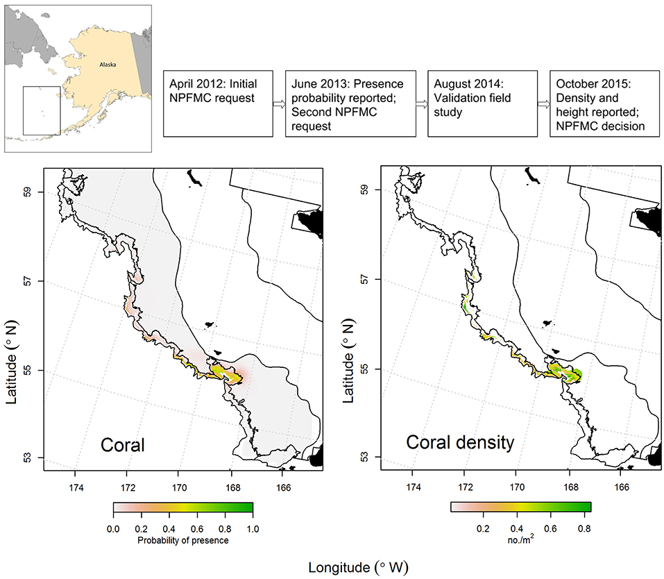
Figure 3. Case Study 1: Eastern Bering Sea Coral Canyons. Timeline (top): Chronology of North Pacific Fishery Management Council (NPFMC) requests, reports, and decision. Plots of predicted presence of coral (adapted from Sigler et al., 2015, left) and predicted density of coral (adapted from Rooper et al., 2016, right). Predicted presence (left) was reported in June 2013 and was based on presence-absence data collected during ecosystem-scale bottom trawl surveys. Predicted density (right) was reported in October 2015 and was based on density data collected during an ecosystem-scale underwater stereo camera survey (the validation study) that was used to update the predicted presence model. Black areas indicate land, and black lines represent boundaries between inner, middle, and outer shelf and slope areas (Sigler et al., 2015).

A validation study was conducted in 2014 using an underwater stereo camera system (Williams et al., 2010). The stereo camera system is highly desirable for region-wide surveys because it can generate large sample sizes (8–10 deployments per day at depths of up to 800 m are routinely achievable) potentially across a large region, where each deployment can sample ~1,100 m² during a 15-min transect. A stratified random survey was conducted where nine strata were identified as 5 canyons, inter-canyon areas, and the outer continental shelf. Sample locations (n = 210 stations) were randomly chosen, but weighted by the probability of coral presence from the bottom trawl survey model, so that on average, locations with higher probability of coral presence were more likely to be chosen. In addition, 10 locations per stratum (n = 90 stations total) were randomly assigned to ensure that unlikely coral habitats also were sampled. During the subsequent fieldwork, a total of 250 locations were sampled (sample locations in the two canyons north of Zhemchug Canyon were largely unsampled due to weather and time constraints). The model validation was conducted by comparing the predictions of the bottom trawl survey model with the observations from the field survey. The new stereo-camera presence data were also used to update the model predictions and used to predict the distribution of density and height of corals and sponges from the underwater stereo camera survey (Rooper et al., 2016; Figure 3); these results were reported to the NPFMC in 2015.

The NPFMC decided against closures of the eastern Bering Sea outer shelf and slope. They concluded that the scientific evidence did not suggest a risk to deep-sea corals, citing the low occurrence and density of deep-sea corals (other than pennatulaceans), the lack of hard substrate to support these corals, and their relatively small size, interpreted as indicating lower vulnerability in these areas to fishery impacts (MacLean et al., 2017). Their conclusion was based on the coral density and height models and the stereo camera survey. The key lessons in this case study in terms of coral modeling were: (1) a model was generated using the best available data (presence and absence from the bottom trawl survey); (2) this model was presented to managers and evaluated by scientists; (3) managers requested more information and validation of the model before using it to make decisions that would affect fisheries; (4) additional data on occurrence, density, and height to validate and improve the model were collected with a sample size and robust statistical design that allowed for inference throughout most of the spatial domain of the model; and (5) these new findings were presented to managers for further evaluation. Throughout the process there were multiple points where updates were provided to managers, stakeholders and scientists so there would be no surprises when each report was formally presented to managers and stakeholders. In this case, a key point was that managers waited for completion of a region-wide field validation study before reaching a decision and were able to reach that decision with more confidence that the deep-sea coral model based on trawl survey data was largely correct (predicting the presence or absence of corals in the camera observations correctly in 72% of cases; Rooper et al., 2016).

Southern California Bight

The Southern California Bight (SCB) has a variety of seafloor habitats and oceanographic conditions that promote a rich diversity of demersal organisms, including a wide variety of fishes (Love et al., 2009) and dense stands of vulnerable DSCS (Tissot et al., 2006; Yoklavich et al., 2011). The SCB is also bordered by one of the most populated areas along the Pacific coast of North America, and the waters of the SCB have been intensively fished both commercially and recreationally to depths over 300 m for at least 40 years (Yoklavich et al., 2011; Salgado et al., 2018). Fishes in the SCB are dominated by rockfish (genus Sebastes; Love et al., 2009), and the two overfished species in the SCB are both within this genus: cowcod (S. levis) and yelloweye (S. ruberrimus). Stakeholder input typically includes a tension between competing goals (maintaining fishing and rebuilding overfished species). Since 2002, management agencies (Pacific Fishery Management Council, NOAA Fisheries, Channel Islands National Marine Sanctuary, and the State of California) have worked together to establish a network of marine reserves with multiple aims, including habitat protection. To conserve and manage the habitats these fish rely on, including DSCS, it is critical to develop SDMs that can provide guidance on the best locations for restrictions on human activities.

In support of these goals, researchers at NOAA's Southwest Fisheries Science Center collected a long time-series (2001–2011) of submersible video from which they built a database of spatially explicit fish and DSCS data (Tissot et al., 2006; Love et al., 2009; Yoklavich et al., 2011) that can be used to build SDMs. All video data recorded during these surveys were processed (i.e., no sub-sampling occurred) and geo-referenced. All fish and invertebrate species were identified to the lowest possible taxonomic level and the length and height of invertebrates were measured to the nearest 5 cm using calibrated lasers. Furthermore, the submersible track locations from all survey dives were recorded, providing data on both DSCS presence and absence. These data were used to quantify the area surveyed and, thus, estimate the density of DSCS. Using these data, Huff et al. (2013) built a GAM to estimate the density of the Christmas tree coral (Antipathes dendrochristos) as a function of multiple environmental covariates (depth, slope, profile, surface productivity, and oceanographic conditions near the seafloor). This GAM was then used to develop a SDM for Christmas tree coral in the SCB (Figure 4).

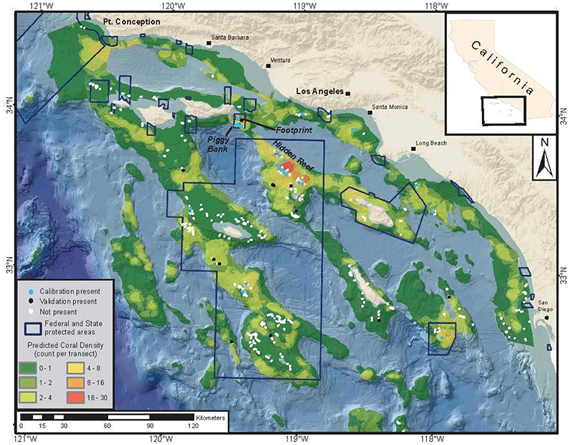
Figure 4. Case Study 2: Southern California Bight. This map depicts coral density (coral colonies per transect group) estimated from a generalized additive model, presence and absence from a calibration dataset and from an independent dataset for Christmas tree corals, along with the boundaries of areas closed to fishing. Mean transect area = 740 m². Figure reproduced with permission from Huff et al. (2013).

These SDMs are extremely valuable to fisheries managers mandated to conserve and manage marine fisheries and their associated habitats, and recent evidence from the SCB has provided further support that multiple species of DSCS are important habitat for demersal fish. Structure-forming DSCS can play an important role in deep-sea benthic communities (D'Onghia, 2019), providing increased prey density (Quattrini et al., 2012) and nursery habitat (Stone, 2006; Baillon et al., 2012). A recent study (Henderson et al., in revision) in the SCB used various spatially explicit analytical methods to identify 8 DSCS taxa that increased the probability of presence for commercially important Sebastes species (S. rufus and S. paucipinis) as well as young-of-year Sebastes, even after accounting for depth and seafloor relief. These results support the classification of these DSCS as essential fish habitat.

The key lessons from this case study are that: (1) it is important to analyze, and geo-reference, all collected data so researchers are not restricted to using presence-only methods; (2) geo-referencing both the fish and DSCS data can provide sufficient data to investigate whether DSCS taxa serve as essential fish habitat within the survey area; and (3) quantifying the area surveyed allows estimation of the density of any DSCS taxa of interest, which provides more management-relevant information than presence-absence estimates. Based on our good practices, we recommend that researchers implement a field-sampling program to validate results from these DSCS SDMs.

Louisville Seamount Chain

The Louisville Seamount Chain is comprised of over 80 seamounts spanning a distance of more than 4,000 km across the South Pacific Ocean. These seamounts are historical and current targets for commercial bottom-trawling fisheries, dominated by the catch of orange roughy (Hoplostethus atlanticus) by New Zealand and Australian flagged vessels (Clark et al., 2016b). These fisheries pose a considerable threat to Vulnerable Marine Ecosystems (VMEs), ecosystems that are particularly susceptible to anthropogenic disturbance as determined by the fragility, functional significance, rarity, and life history traits of their components (FAO (Food and Agriculture Organization of the United Nations), 2009). The seamount chain lies outside of national jurisdiction, and fisheries management is conducted by the South Pacific Regional Fisheries Management Organization (SPRFMO), an intergovernmental agency mandated by the United Nations to protect VMEs while also ensuring the future of sustainable fisheries [UNGA (United Nations General Assembly), 2006]. SPRFMO has implemented two primary interim measures to protect VMEs. First, a move-on rule that requires vessels to cease fishing within 5 nautical miles of an encountered VME, usually triggered by the bycatch of a VME indicator taxon. Indicator taxa are those that are vulnerable to fishing gear, functionally significant (e.g., habitat creators), rare or endemic, or low productivity species (e.g., slow growth rate, low fecundity) (Parker et al., 2009). Second, SPRFMO enacted a series of large (20 arc-min) closures in areas with a historically low fishing impact. However, the underlying effectiveness and real-world implementation of these interim measures has been questioned (Penney and Guinotte, 2013), and SPRFMO is actively pursuing long-term replacement measures with a focus on more effective spatial closures.

Rowden et al. (2017) used a variety of habitat suitability modeling techniques to map the distribution of VMEs across the Louisville Seamount Chain in order to support the improved spatial management of the region's fisheries (Figure 5). The authors built on a series of broad-scale regional models that generally highlighted the seamount chain as being highly suitable for a variety of VME taxa (Anderson et al., 2016a,b; Georgian et al., 2019). Three VME indicator taxa were modeled at a high spatial resolution (25 m) on seven seamounts: the stony coral Solenosmilia variabilis, sea stars (Brisingida), and crinoids (Crinoidea). Biological data were collected during a cruise designed to ground-truth the regional models using a random-stratified survey. Environmental data (backscatter and a large suite of multi-scale terrain metrics) were derived from high-resolution multibeam surveys conducted during the cruise. Both presence-absence and abundance ensemble models were constructed using the performance-weighted average of BRT, GAM, and RF models. Model performance was assessed using a 70–30 cross-validation approach and by bootstrapping the input presence-absence and abundance data to estimate model uncertainty (CV) (sensu Anderson et al., 2016b). To reduce the effect of spatial autocorrelation on model performance, the residual autocovariate was calculated from the residuals of preliminary models (Crase et al., 2012).

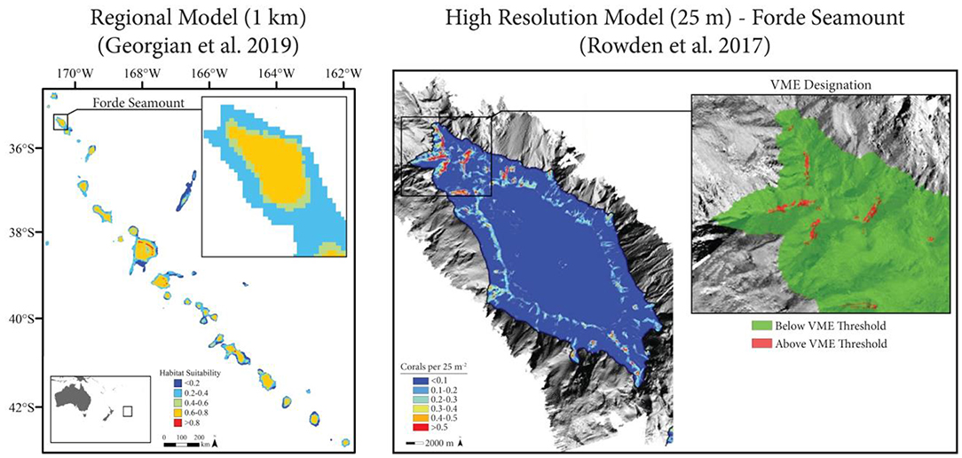
Figure 5. Case Study 3: Louisville Seamount Chain (Rowden et al., 2017). Left: Regional habitat suitability models (1 km, adapted from Georgian et al., 2019) indicated high suitability for the stony coral Solenosmilia variabilis throughout the Louisville Seamount Chain. Right: High resolution models (25 m, adapted from Rowden et al., 2017) were constructed for six individual seamounts (Forde Seamount shown), and Vulnerable Marine Ecosystems (VMEs) were identified based on a threshold applied to S. variabilis abundance models.

Ultimately, Rowden et al. (2017) demonstrated that the modeled seamounts constituted less suitable habitat than previously predicted by broader scale regional models. However, small sections of each seamount (<0.1% of the modeled area) contained highly suitable habitat for one or more VME indicator taxa. These results suggest that an optimal management solution that prioritizes VME protection while simultaneously allowing fishery access to less suitable areas may exist for the Louisville Seamount Chain. The modeling approach used provides several useful lessons for future modeling studies, particularly when resource management is the eventual goal: (1) it is imperative to revise and improve models when new or better data become available; (2) high resolution models continue to be important tools that capture spatial patterns that may differ from broad scale models and have the potential to significantly alter spatial management plans (e.g., Dolan et al., 2008); (3) true presence-absence and abundance models should be used when the data allow, given their generally improved performance and easier ecological interpretation (see Yackulic et al., 2013); (4) sampling bias and spatial autocorrelation, although frequently ignored in modeling studies (see Dormann, 2007), should be accounted for using either statistical approaches (e.g., Georgian et al., 2019) or an appropriate survey structure (e.g., Rowden et al., 2017); (5) ensemble models are powerful tools that avoid overreliance on the underlying structure and assumptions of different modeling techniques (Robert et al., 2016); and (6) calculating a spatial measure of model uncertainty allows decision makers to prioritize management measures based on both the suitability of a given area as well as the confidence of the model at that site (Anderson et al., 2016a,b).

Conclusion

The geographic scale of potential human impacts on DSCS combined with the localized nature of available information about the spatial distributions of these species necessitates the use of SDMs by managers looking to assess and mitigate these impacts. Here we have described some good practices for developing such models and making use of them in management decision-making (Table 1). In particular, we recommend that SDMs move beyond presence-only models to include measurements of DSCS presence-absence, abundance, and height; these predictions are easier to validate and/or test in subsequent targeted field-sampling programs and are more easily understood by managers and stakeholders. Model predictions should be presented with associated measures of uncertainty, where this uncertainty is used to weight predictions from different models within an ensemble of SDMs. We strongly encourage consideration of scale in DSCS SDMs used in management decision-making, including spatial (e.g., large marine ecosystem or management region, or more localized marine protected area or ecologically sensitive location) and temporal (e.g., short-term response to specific impacts or long-term) scale (Lecours et al., 2015). We recognize the logistical challenges and expense of collecting data on DSCS and appreciate that it may be impractical to implement all of these good practices in every situation. Indeed, the case studies presented here sometimes required significant financial resources, and they did not necessarily incorporate every one of our good practices. Nevertheless, we hope that these good practices provide useful guidance for future DSCS data collections and SDMs, especially models that will be used to inform management of human activities in the deep sea.

Author Contributions

All authors listed have made a substantial, direct and intellectual contribution to the work, and approved it for publication.

Funding

This manuscript is based on the conclusions of a workshop funded by the NOAA Deep Sea Coral Research and Technology Program as part of their West Coast Deep-Sea Coral Initiative (WCDSCI). Support for AW was provided by CSS, Inc. under NOAA contract EA-133C-14-NC-1384.

Conflict of Interest

AW and MP were employed by the company CSS, Inc.

The remaining authors declare that the research was conducted in the absence of any commercial or financial relationships that could be construed as a potential conflict of interest.

Acknowledgments

We thank C. Caldow, MC, and the rest of the Initiative Steering Committee for supporting the workshop, and G. Hoff and A. O. Shelton for contributions during the workshop. C. Caldow, L. Gilbane, G. Hoff, C. Menza, M. Mueller, and three reviewers provided helpful comments that improved upon an earlier version of the manuscript. Support for AW and MP was provided by CSS, Inc. under NOAA contract EA-133C-14-NC-1384. The Alaska research presented as Case Study 1 was funded by NOAA's DSCRTP, NOAA's Alaska Fisheries Science Center's Habitat and Ecological Processes Research Program, and NOAA's Cooperative Research Program. The Southern California Bight (SCB) research presented as Case Study 2 was partially drawn from an article co-authored by M. M. Yoklavich, M. S. Love, D. L. Watters, F. Chai, and S. T. Lindley. Supplemental funds for the SCB research were provided through grants from NOAA's DSCRTP. The South Pacific research presented as Case Study 3 was first published by Rowden et al. (2017) and Georgian et al. (2019) and was funded by the New Zealand Ministry for Business, Innovation, and Employment, and by the New Zealand Ministry for Primary Industries (MPI). The scientific results and conclusions, as well as any views or opinions expressed herein, are those of the authors and do not necessarily reflect those of the U.S. Government. Any use of trade, firm, or product names is for descriptive purposes only and does not imply endorsement by the U.S. Government.

Supplementary Material

The Supplementary Material for this article can be found online at: https://www.frontiersin.org/articles/10.3389/fmars.2020.00303/full#supplementary-material

Footnotes

References

Allouche, O., Tsoar, A., and Kadmon, R. (2006). Assessing the accuracy of species distribution models: prevalence, kappa and the true skill statistic (TSS). J. Appl. Ecol. 43, 1223–1232. doi: 10.1111/j.1365-2664.2006.01214.x
Anderson, O. F., Guinotte, J. M., Rowden, A. A., Clark, M. R., Mormede, S., Davies, A. J., et al. (2016a). Field validation of habitat suitability models for vulnerable marine ecosystems in the South Pacific Ocean: implications for the use of broad-scale models in fisheries management. Ocean Coast. Manag. 120, 110–126. doi: 10.1016/j.ocecoaman.2015.11.025
Anderson, O. F., Guinotte, J. M., Rowden, A. A., Tracey, D. M., Mackay, K. A., and Clark, M. R. (2016b). Habitat suitability models for predicting the occurrence of vulnerable marine ecosystems in the seas around New Zealand. Deep Sea Res. I 115, 265–292. doi: 10.1016/j.dsr.2016.07.006
Auster, P. J. (2005). “Are deep-water corals important habitats for fishes?,” in Cold-water Corals and Ecosystems, eds A. Freiwald, J. M. Roberts (Berlin: Springer), 747–760. doi: 10.1007/3-540-27673-4_39
Baillon, S., Hamel, J.-F., Wareham, V. E., and Mercier, A. (2012). Deep cold-water corals as nurseries for fish larvae. Front. Ecol. Environ. 10, 351–356. doi: 10.1890/120022
Bargain, A., Foglini, F., Pairaud, I., Bonaldo, D., Carniel, S., Angeletti, L., et al. (2018). Predictive habitat modeling in two Mediterranean canyons including hydrodynamic variables. Progr. Oceanogr. 169, 151–168. doi: 10.1016/j.pocean.2018.02.015
Bauer, L., Poti, M., Costa, B., Wagner, D., Parrish, F., Donovan, M., and Kinlan, B. (2016). “Benthic habitats and corals,” in Marine biogeographic assessment of the Main Hawaiian Islands, Bureau of Ocean Energy Management and National Oceanic and Atmospheric Administration. OCS Study BOEM 2016-035 and NOAA Technical Memorandum NOS NCCOS 214, eds B. M. Costa, M. S. Kendall (Silver Spring, MD: National Ocean Service), 57–136.
Brown, C. J., Smith, S. J., Lawton, P., and Anderson, J. T. (2011). Benthic habitat mapping: a review of progress towards improved understanding of the spatial ecology of the seafloor using acoustic techniques. Estuar. Coast. Shelf Sci. 92, 502–520. doi: 10.1016/j.ecss.2011.02.007
Buhl-Mortensen, L., Buhl-Mortensen, P., Dolan, M. F. J., Dannheim, J., Bellec, V., and Holte, B. (2012). Habitat complexity and bottom fauna composition at different scales on the continental shelf and slope of northern Norway. Hydrobiologia 685, 191–219. doi: 10.1007/s10750-011-0988-6
Buhl-Mortensen, L., Vanreusel, A., Gooday, A. J., Levin, L. A., Priede, I. G., Buhl-Mortensen, P., et al. (2010). Biological structures as a source of habitat heterogeneity and biodiversity on the deep ocean margins. Mar. Ecol. 31, 21–50. doi: 10.1111/j.1439-0485.2010.00359.x
Bunnefeld, N., Hoshino, E., and Milner-Gulland, E. J. (2011). Management strategy evaluation: a powerful tool for conservation? Trends Ecol. Evol. 26, 441–447. doi: 10.1016/j.tree.2011.05.003
Cathalot, C., Van Oevelen, D., Cox, T. J. S., Kutti, T., Lavaleye, M., Duineveld, G., et al. (2015). Cold-water coral reefs and adjacent sponge grounds: hotspots of benthic respiration and organic carbon cycling in the deep sea. Front. Mar. Sci. 2:37. doi: 10.3389/fmars.2015.00037
Clark, M. R., Althaus, F., Schlacher, T. A., Williams, A., Bowden, D. A., and Rowden, A. A. (2016a). The impacts of deep-sea fisheries on benthic communities: a review. ICES J. Mar. Sci. 73(Suppl.1), i51–i69. doi: 10.1093/icesjms/fsv123
Clark, M. R., McMillan, P. J., Anderson, O. F., and Roux, M.-J. (2016b). Stock Management Areas for Orange Roughy (Hoplostethus atlanticus) in the Tasman Sea and Western South Pacific Ocean. Wellington: New Zealand Fisheries Assessment Report 2016/19.
Conrath, C. L., Rooper, C. N., Wilborn, R. E., Knoth, B. A., and Jones, D. T. (2019). Seasonal habitat use and community structure of rockfishes in the Gulf of Alaska. Fish. Res. 219:105331. doi: 10.1016/j.fishres.2019.105331
Convention on Biological Diversity (CBD) (2010). Report of the Expert Workshop on Scientific and Technical Guidance on the Use of Biogeographic Classification Systems and Identification of Marine Areas Beyond National Jurisdiction in Need of Protection. UNEP/CBD/SBSTTA/14/INF/4. Available online at: https://www.cbd.int/doc/meetings/sbstta/sbstta-14/information/sbstta-14-inf-04-en.pdf
Crase, B., Liedloff, A. C., and Wintle, B. A. (2012). A new method for dealing with residual spatial autocorrelation in species distribution models. Ecography 35, 879–888. doi: 10.1111/j.1600-0587.2011.07138.x
Davies, A. J., and Guinotte, J. M. (2011). Global habitat suitability for framework-forming cold-water corals. PLoS ONE 6:e18483. doi: 10.1371/journal.pone.0018483
Dolan, M. F. J., Grehan, A. J., Guinan, J. C., and Brown, C. (2008). Modelling the local distribution of cold-water corals in relation to bathymetric variables: adding spatial context to deep-sea video data. Deep Sea Res. I 55, 1564–1579. doi: 10.1016/j.dsr.2008.06.010
D'Onghia, G. (2019). “Cold-water corals as shelter, feeding and life-history critical habitats for fish species: Ecological interactions and fishing impact,” in Mediterranean cold-water corals: Past, present and future. Coral reefs of the world, Vol. 9, eds C. Orejas, C. Jiménez (Cham: Springer). 335–356. doi: 10.1007/978-3-319-91608-8_30
D'Onghia, G., Calculli, C., Capezzuto, F., Carlucci, R., Carluccio, A., Maiorano, P., et al. (2016). New records of cold-water coral sites and fish fauna characterization of a potential network existing in the Mediterranean Sea. Mar. Ecol. 37,1398–1422. doi: 10.1111/maec.12356
Dormann, C. F. (2007). Effects of incorporating spatial autocorrelation into the analysis of species distribution data. Glob. Ecol. Biogeogr. 16, 129–138. doi: 10.1111/j.1466-8238.2006.00279.x
Dormann, C. F., McPherson, J. M., Araújo, M. B., Bivand, R., Bolliger, J., Carl, G., et al. (2007). Methods to account for spatial autocorrelation in the analysis of species distributional data: a review. Ecography 30, 609–628. doi: 10.1111/j.2007.0906-7590.05171.x
Dove, D., Weijerman, M., Grüss, A., Acoba, T., and Smith, J. R. (2020). “Substrate mapping to inform ecosystem science and marine spatial planning around the Main Hawaiian Islands,” in Seafloor Geomorphology as Benthic Habitat: GeoHab Atlas of Seafloor Geomorphic Features and Benthic Habitat, 2nd Edn, eds P. Harris and E. Baker (London: Elsevier). 619–640. doi: 10.1016/B978-0-12-814960-7.00037-3
Du Preez, C., and Tunnicliffe, V. (2011). Shortspine thornyhead and rockfish (Scorpaenidae) distribution in response to substratum, biogenic structures and trawling. Mar. Ecol. Prog. Ser. 425, 217–231. doi: 10.3354/meps09005
El-Gabbas, A., and Dormann, C. F. (2018). Improved species-occurrence predictions in data-poor regions: using large-scale data and bias correction with down-weighted Poisson regression and Maxent. Ecography 41, 1161–1172. doi: 10.1111/ecog.03149
Elith, J., Phillips, S. J., Hastie, T., Dudík, M., Chee, Y. E., and Yates, C. J. (2011). A statistical explanation of MaxEnt for ecologists. Diversity Distrib. 17, 43–57. doi: 10.1111/j.1472-4642.2010.00725.x
Etnoyer, P. J., Wagner, D., Fowle, H. A., Poti, M., Kinlan, B., Georgian, S. E., et al. (2018). Models of habitat suitability, size, and age-class structure for the deep-sea black coral Leiopathes glaberrima in the Gulf of Mexico. Deep Sea Res. II 150, 218–228. doi: 10.1016/j.dsr2.2017.10.008
FAO (Food Agriculture Organization of the United Nations) (2009). International Guidelines for the Management of Deep-Sea Fisheries in the High-Seas. Available online at: http://www.fao.org/fishery/topic/166308/en
Fiechter, J., Edwards, C. A., and Moore, A. M. (2018). Wind, circulation, and topographic effects on alongshore phytoplankton variability in the California Current. Geophys. Res. Lett. 45, 3238–3245. doi: 10.1002/2017GL076839
Fithian, W., Elith, J., Hastie, T., and Keith, D. A. (2015). Bias correction in species distribution models: pooling survey and collection data for multiple species. Methods Ecol. Evol. 6, 424–438. doi: 10.1111/2041-210X.12242
Fletcher, R. J. Jr., Hefley, T. J., Robertson, E. P., Zuckerberg, B., McCleery, R. A., and Dorazio, R.M. (2019). A practical guide for combining data to model species distributions. Ecology 100:e02710. doi: 10.1002/ecy.2710
GEBCO (General Bathymetric Chart of the Oceans) Compilation Group (2019). GEBCO_2019 Grid. doi: 10.5285/836f016a-33be-6ddc-e053-6c86abc0788e
Georgian, S. E., Anderson, O. F., and Rowden, A. A. (2019). Ensemble habitat suitability modeling of vulnerable marine ecosystem indicator taxa to inform deep-sea fisheries management in the South Pacific Ocean. Fish. Res. 211, 256–274. doi: 10.1016/j.fishres.2018.11.020
Georgian, S. E., Shedd, W., and Cordes, E. E. (2014). High-resolution ecological niche modelling of the cold-water coral Lophelia pertusa in the Gulf of Mexico. Mar. Ecol. Prog. Ser. 506, 145–161. doi: 10.3354/meps10816
Grüss, A., Drexler, M. D., Chancellor, E., Ainsworth, C. H., Gleason, J. S., Tirpak, J. M., et al. (2019). Representing species distributions in spatially-explicit ecosystem models from presence-only data. Fish. Res. 210, 89–105. doi: 10.1016/j.fishres.2018.10.011
Grüss, A., Perryman, H. A., Babcock, E. A., Sagarese, S. R., Thorson, J. T., Ainsworth, C. H., et al. (2018). Monitoring programs of the US Gulf of Mexico: inventory, development and use of a large monitoring database to map fish and invertebrate spatial distributions. Rev. Fish Biol. Fish. 28, 667–691. doi: 10.1007/s11160-018-9525-2
Grüss, A., and Thorson, J. (2019). Developing spatio-temporal models using multiple data types for evaluating population trends and habitat usage. ICES J. Mar. Sci. 76, 1748–1761. doi: 10.1093/icesjms/fsz075
Guinotte, J. M., Georgian, S., Kinlan, B. P., Poti, M., and Davies, A. J. (2017). “Predictive habitat modeling for deep-sea corals in U.S. waters,” in The State of Deep-Sea Coral and Sponge Ecosystems of the United States. NOAA Technical Memorandum NMFS-OHC-4, eds T. F. Hourigan, P. J. Etnoyer, and S. D. Cairns (Silver Spring, MD: National Marine Fisheries Service). 213–235.
Guisan, A., Thuiller, W., and Zimmermann, N. (2017). Habitat suitability and distribution models: With Applications in R. Cambridge, U.K: Cambridge University Press. doi: 10.1017/9781139028271
Hermann, A., Ladd, C., Cheng, W., Curchitser, E., and Hedstrom, K. (2016). A model-based examination of multivariate physical modes in the Gulf of Alaska. Deep Sea Res. II 132, 68–89. doi: 10.1016/j.dsr2.2016.04.005
Hirzel, A., and Guisan, A. (2002). Which is the optimal sampling strategy for habitat suitability modelling. Ecol. Model. 157, 331–341. doi: 10.1016/S0304-3800(02)00203-X
Hogg, M. M., Tendal, O. S., Conway, K. W., Pomponi, S. A., van Soest, R. W. M., Gutt, J., et al. (2010). Deep-Sea Sponge Grounds: Reservoirs of biodiversity. UNEPWCMC Biodiversity Series no. 32. UNEP-WCMC, Cambridge.
Hourigan, T. F. (2014). “A strategic approach to address fisheries impacts on deep-sea coral ecosystems” in Interrelationships Between Corals and Fisheries, ed S. A. Bortone (Boca Raton, FL: CRC Press) 127–145. doi: 10.1201/b17159-9
Hourigan, T. F., Etnoyer, P. J., and Cairns, S. D., (eds.). (2017). “The state of deep-sea coral and sponge ecosystems of the United States,” NOAA Technical Memorandum NMFS-OHC-4. (Silver Spring, MD: National Marine Fisheries Service), p. 467.
Huff, D. D., Yoklavich, M. M., Love, M. S., Watters, D. L., Chai, F., and Lindley, S. T. (2013). Environmental factors that influence the distribution, size, and biotic relationships of the Christmas tree coral Antipathes dendrochristos in the Southern California Bight. Mar. Ecol. Prog. Ser. 494, 159–177. doi: 10.3354/meps10591
Hughes Clarke, J. E. (2015). Multispectral acoustic backscatter from multibeam, improved classification potential. Proceedings of United States Hydrographic Conference, National Harbor, Maryland, March 16–19.
Isaac, N. J., van Strien, A. J., August, T. A., de Zeeuw, M. P., and Roy, D. B. (2014). Statistics for citizen science: extracting signals of change from noisy ecological data. Method. Ecol. Evol. 5, 1052–1060. doi: 10.1111/2041-210X.12254
Jakobsson, M., Mayer, L., Coakley, B., Dowdeswell, J. A., Forbes, S., Fridman, B., et al. (2012). The International Bathymetric Chart of the Arctic Ocean (IBCAO) Version 3.0. Geophys. Res. Lett. 39:L12609. doi: 10.1029/2012GL052219
Jimenez-Valverde, A. (2012). Insights into the area under the receiver operating characteristic curve (AUC) as a discrimination measure in species distribution modelling. Glob. Ecol. Biogeogr. 21, 498–507. doi: 10.1111/j.1466-8238.2011.00683.x
Kenchington, E., Power, D., and Koen-Alonso, M. (2013). Associations of demersal fish with sponge grounds on the continental slopes of the northwest Atlantic. Mar. Ecol. Prog. Ser. 477, 217–230. doi: 10.3354/meps10127
Kinlan, B. P., Poti, M., Drohan, A. F., Packer, D. B., Dorfman, D. S., and Nizinski, M. S. (2020). Predictive modeling of suitable habitat for deep-sea corals offshore the northeast United States. Deep Sea Res. I 158:103229. doi: 10.1016/j.dsr.2020.103229
Kuhn, M., and Johnson, K. (2013). Applied predictive modeling. Springer Science and Business Media, New York, NY.
Laman, N., Kotwicki, S., and Rooper, C. N. (2015). Sponge and coral morphology influences the distribution of Pacific ocean perch life stages. Fish. Bull. 113, 270–289. doi: 10.7755/FB.113.3.4
Lecours, V., Devillers, R., Schneider, D. C., Lucieer, V. L., Brown, C. J., and Edinger, E. N. (2015). Spatial scale and geographic context in benthic habitat mapping: review and future directions. Mar. Ecol. Prog. Ser. 535, 259–284. doi: 10.3354/meps11378
Legendre, P. (1993). Spatial autocorrelation: trouble or new paradigm? Ecology 74, 1659–1673. doi: 10.2307/1939924
Levin, P. S., Fogarty, M. J., Murawski, S. A., and Fluharty, D. (2009). Integrated ecosystem assessments: Developing the scientific basis for ecosystem-based management of the ocean. PLOS Biol. 7:e1000014. doi: 10.1371/journal.pbio.1000014
Liu, C., Berry, P. M., Dawson, T. P., and Pearson, R. G. (2005). Selecting thresholds of occurrence in the prediction of species distributions. Ecography 28, 385–393. doi: 10.1111/j.0906-7590.2005.03957.x
Lo Iacono, C., Robert, K., Gonzalez-Villanueva, R., Gori, A., Gili, J.-M., and Orejas, C. (2018). Predicting cold-water coral distribution in the Cap de Creus Canyon (NW Mediterranean): Implications for marine conservation planning. Progr. Oceanogr. 169, 169–180. doi: 10.1016/j.pocean.2018.02.012
Lobo, J. M., Jiménez-Valverde, A., and Real, R. (2008). AUC: a misleading measure of the performance of predictive distribution models. Glob. Ecol. Biogeogr. 17, 145–151. doi: 10.1111/j.1466-8238.2007.00358.x
Love, M. S., Yoklavich, M., and Schroeder, D. M. (2009). Demersal fish assemblages in the Southern California Bight based on visual surveys in deep water. Environ. Biol. Fishes 84, 55–68. doi: 10.1007/s10641-008-9389-8
Lurton, X., and Lamarche, G., (eds.). (2015). Backscatter Measurements by Seafloor-Mapping Sonars. Guidelines and Recommendations. GeoHab Backscatter Working Group.
MacLean, S. A., Rooper, C. N., and Sigler, M. F. (2017). Corals, canyons, and conservation: science based fisheries management decisions in the Eastern Bering Sea. Front. Mar. Sci. 4:142. doi: 10.3389/fmars.2017.00142
Maldonado, M., Aguilar, R., Bannister, R. J., Bell, J. J., Conway, K. W., Dayton, P. K., et al. (2017). “Sponge grounds as key marine habitats: a synthetic review of types, structure, functional roles, and conservation concerns,” in Marine Animal forests: The ecology of benthic biodiversity hotspots, eds S. Rossi, L. Bramanti, A. Gori, C. Orejas Saco del Valle (Switzerland: Springer International Publishing). 145–183.
Malecha, P. W., Stone, R. P., and Heifetz, J. (2005). “Living substrate in Alaska: distribution, abundance, and species associations,” in Benthic Habitats and the Effects of Fishing, eds P.W. Barnes and J. P. Thomas (41, Bethesda, Maryland: Am. Fish. Soc. Symp.). 289–299.
Merow, C., Allen, J. M., Aiello-Lammens, M., and Silander, J. A. Jr. (2016). Improving niche and range estimates with Maxent and point process models by integrating spatially explicit information. Global Ecol. Biogeogr. 25, 1022–1036. doi: 10.1111/geb.12453
Miller, D. A. W., Pacifici, K., Sanderlin, J. S., and Reich, B. J. (2019). The recent past and promising future for data integration methods to estimate species' distributions. Method. Ecol. Evol. 10, 22–37. doi: 10.1111/2041-210X.13110
Ovaskainen, O., Tikhonov, G., Norberg, A., Guillaume Blanchet, F., Duan, L., Dunson, D., et al. (2017). How to make more out of community data? A conceptual framework and its implementation as models and software. Ecol. Lett. 20, 561–576. doi: 10.1111/ele.12757
Parker, S., Penney, A., and Clark, M. (2009). Detection criteria for managing trawl impacts on vulnerable marine ecosystems in high seas fisheries of the South Pacific Ocean. Mar. Ecol. Prog. Ser. 397, 309–317. doi: 10.3354/meps08115
Peel, S. L., Hill, N. A., Foster, S. D., Wotherspoon, S. J., Ghiglione, C., and Schiaparelli, S. (2019). Reliable species distributions are obtainable with sparse, patchy and biased data by leveraging over species and data types. Methods Ecol. Evol. 10, 1002–1014. doi: 10.1111/2041-210X.13196
Penney, A. J., and Guinotte, J. M. (2013). Evaluation of New Zealand's high-seas bottom trawl closures using predictive habitat models and quantitative risk assessment. PLoS ONE 8:e82273. doi: 10.1371/journal.pone.0082273
Pirtle, J. L., Shotwell, S. K., Zimmermann, M., Reid, J. A., and Golden, N. (2019). Habitat suitability models for groundfish in the Gulf of Alaska. Deep Sea Res. II 165, 303–321. doi: 10.1016/j.dsr2.2017.12.005
Pirtle, J. L., Weber, T. C., Wilson, C. D., and Rooper, C. N. (2015). Assessment of trawlable and untrawlable seafloor using multibeam-derived metrics. Method. Oceanogr. 12, 18–35. doi: 10.1016/j.mio.2015.06.001
Quattrini, A. M., Ross, S. W., Carlson, M. C., and Nizinski, M. S. (2012). Megafaunal-habitat associations at a deep-sea coral mound off North Carolina, USA. Mar. Biol. 159, 1079–1094. doi: 10.1007/s00227-012-1888-7
Renner, I. W., Elith, J., Baddeley, A., Fithian, W., Hastie, T., Phillips, S. J., et al. (2015). Point process models for presence-only analysis. Methods Ecol. Evol. 6, 366–379. doi: 10.1111/2041-210X.12352
Robert, K., Jones, D. O. B., Roberts, J. M., and Huvenne, V. A. I. (2016). Improving predictive mapping of deep-water habitats: Considering multiple model outputs and ensemble techniques. Deep Sea Res. I 113, 80–89. doi: 10.1016/j.dsr.2016.04.008
Roberts, J. M., Wheeler, A., Freiwald, A., and Cairns, S. (2009). Cold-Water Corals: the Biology and Geology of Deep-Sea Coral Habitats. Cambridge: Cambridge University Press. doi: 10.1017/CBO9780511581588
Rooper, C. N., Etnoyer, P. J., Stierhoff, K. L., and Olson, J. V. (2017b). “Effects of fishing gear on deep-sea corals and sponges in U.S. waters,” in The State of Deep-Sea Coral and Sponge Ecosystems of the United States. NOAA Technical Memorandum NMFS-OHC-4, eds T. F. Hourigan, P. J. Etnoyer and S. D. Cairns (Silver Spring, MD), 93–111.
Rooper, C. N., Hoff, G. R., Stevenson, D. E., Orr, J. W., and Spies, I. B. (2019). Skate egg nursery habitat in the eastern Bering Sea: a predictive model. Mar. Ecol. Prog. Ser. 609, 163–178. doi: 10.3354/meps12809
Rooper, C. N., Sigler, M. F., Goddard, P., Malecha, P., Towler, R., Williams, K., et al. (2016). Validation and improvement of species distribution models for structure-forming invertebrates in the eastern Bering Sea with an independent survey. Mar. Ecol. Prog. Ser. 551, 117–130. doi: 10.3354/meps11703
Rooper, C. N., Wilborn, R., Goddard, P., Williams, K., Towler, R., and Hoff, G. R. (2018). Validation of deep-sea coral and sponge distribution models in the Aleutian Islands, Alaska. ICES J. Mar. Sci. 75, 199–209. doi: 10.1093/icesjms/fsx087
Rooper, C. N., Zimmermann, M., and Prescott, M. M. (2017a). Comparison of modeling methods to predict the spatial distribution of deep-sea coral and sponge in the Gulf of Alaska. Deep Sea Res. I 126, 148–161. doi: 10.1016/j.dsr.2017.07.002
Rooper, C. N., Zimmermann, M., Prescott, M. M., and Hermann, A. J. (2014). Predictive models of coral and sponge distribution, abundance and diversity in bottom trawl surveys of the Aleutian Islands, Alaska. Mar. Ecol. Prog. Ser. 503, 157–176. doi: 10.3354/meps10710
Rossi, S., Bramanti, L., Gori, A., and Orejas, C. (2017). “An overview of the animal forests of the world,” in Marine animal forests: the ecology of benthic biodiversity hotspots, eds S. Rossi, L. Bramanti, A. Gori, and C. Orejas (Switzerland: Springer International Publishing). 1–26. doi: 10.1007/978-3-319-17001-5_1-1
Rowden, A. A., Anderson, O. F., Georgian, S. E., Bowden, D. A., Clark, M. R., Pallentin, A., et al. (2017). High-resolution habitat suitability models for the conservation and management of vulnerable marine ecosystems on the Louisville Seamount Chain, South Pacific Ocean. Front. Mar. Sci. 4:335. doi: 10.3389/fmars.2017.00335
Salgado, E. J., Nehasil, S. E., and Etnoyer, P. J. (2018). Distribution of deep-water corals, sponges, and demersal fisheries landings in Southern California, USA: implications for conservation priorities. PeerJ 6:e5697. doi: 10.7717/peerj.5697
Shelton, A. O., Thorson, J. T., Ward, E. J., and Feist, B. E. (2014). Spatial semiparametric models improve estimates of species abundance and distribution. Can. J. Fish. Aquat. Sci. 71, 1655–1666. doi: 10.1139/cjfas-2013-0508
Sigler, M. F., Rooper, C. N., Hoff, G. R., Stone, R. P., McConnaughey, R. A., and Wilderbuer, T. K. (2015). Faunal features of submarine canyons on the eastern Bering Sea slope. Mar. Ecol. Prog. Ser. 526, 21–40. doi: 10.3354/meps11201
Stone, R. P. (2006). Coral habitat in the Aleutian Islands of Alaska: depth distribution, fine-scale species associations, and fisheries interactions. Coral Reefs 25, 229–238. doi: 10.1007/s00338-006-0091-z
Stone, R. P. (2014). The ecology of deep-sea coral and sponge habitats of the central Aleutian Islands of Alaska. U.S. Department of Commerce, NOAA Professional Paper NMFS 16. 52. doi: 10.7755/PP.16
Thorson, J. T., and Barnett, L. A. (2017). Comparing estimates of abundance trends and distribution shifts using single-and multispecies models of fishes and biogenic habitat. ICES J. Mar. Sci. 74, 1311–1321. doi: 10.1093/icesjms/fsw193
Tissot, B. N., Yoklavich, M. M., Love, S., York, K., and Amend, M. (2006). Benthic invertebrates that form habitat structures on deep banks off southern California, with special reference to deep sea coral. Fish. Bull. 104, 167–181.
UNGA (United Nations General Assembly) (2006). Resolution 61/105. Sustainable Fisheries, Including Through the 1995. Agreement for the Implementation of the Provisions of the United Nations Convention on the Law of the Sea of 10 December 1982. Relating to the Conservation and Management of Straddling Fish Stocks and Highly Migratory Fish Stocks, and Related Instruments.
Valavi, R., Elith, J., Lahoz-Monfort, J. J., and Guillera-Arroita, G. (2019). blockCV: an R package for generating spatially or environmentally separated folds for k-fold cross-validation of species distribution models. Method. Ecol. Evol. 10, 225–232. doi: 10.1111/2041-210X.13107
Vierod, A. D., Guinotte, J. M., and Davies, A. J. (2014). Predicting the distribution of vulnerable marine ecosystems in the deep sea using presence-background models. Deep Sea Res. II 99, 6–18. doi: 10.1016/j.dsr2.2013.06.010
Weber, T. C., Rooper, C., Butler, J., Jones, D., and Wilson, C. (2013). Seabed classification for trawlability determined with a multibeam echo sounder on Snakehead Bank in the Gulf of Alaska. Fish. Bull. 111, 68–77. doi: 10.7755/FB.111.1.6
Weijerman, M., Grüss, A., Dove, D., Asher, J., Williams, I. D., Kelley, C., et al. (2019). Shining a light on the composition and distribution patterns of mesophotic and subphotic fish communities in Hawai'i. Mar. Ecol. Prog. Ser. 630, 161–182. doi: 10.3354/meps13135
Williams, B. K., and Brown, E. D. (2019). Sampling and analysis frameworks for inference in ecology. Method. Ecol. Evol. 10, 1832–1842. doi: 10.1111/2041-210X.13279
Williams, K., Rooper, C. N., and Towler, R. (2010). Use of stereo camera systems for assessment of rockfish abundance in untrawlable areas and for recording pollock behavior during midwater trawls. Fish. Bull. 108, 352–362.
Wilson, M. F. J., O'Connell, B., Brown, C., Guinan, J. C., and Grehan, A. J. (2007). Multiscale terrain analysis of multibeam bathymetry data for habitat mapping on the continental slope. Marine Geodesy 30, 3–35. doi: 10.1080/01490410701295962
Woolley, S. N. C., McCallum, A. W., Wilson, R., O'Hara, T. D., and Dunstan, P. K. (2013). Fathom out: biogeographical subdivision across the Western Australian continental margin - a multispecies modelling approach. Diversity Distrib. 19, 1506–1517. doi: 10.1111/ddi.12119
Yackulic, C. B., Chandler, R., Zipkin, E. F., Royle, J. A., Nichols, J. D., Campbell Grant, E. H., et al. (2013). Presence-only modelling using MAXENT: when can we trust the inferences? Method. Ecol. Evol. 4, 236–243. doi: 10.1111/2041-210x.12004
Yoklavich, M. M., Laidig, T., Krigsman, L., Taylor, A., Watters, D., Love, M., et al. (2011). A characterization of the coral and sponge community on Piggy Bank seamount in southern California from a survey using a remotely operated vehicle. A report to NOAA Deep-sea Coral Research and Technology Program. 63p.
Keywords: corals, deep sea, good practices, management, species distribution models, sponges
Citation: Winship AJ, Thorson JT, Clarke ME, Coleman HM, Costa B, Georgian SE, Gillett D, Grüss A, Henderson MJ, Hourigan TF, Huff DD, Kreidler N, Pirtle JL, Olson JV, Poti M, Rooper CN, Sigler MF, Viehman S and Whitmire CE (2020) Good Practices for Species Distribution Modeling of Deep-Sea Corals and Sponges for Resource Management: Data Collection, Analysis, Validation, and Communication. Front. Mar. Sci. 7:303. doi: 10.3389/fmars.2020.00303
Received: 09 January 2020; Accepted: 15 April 2020;
Published: 12 May 2020.
Edited by:
Santiago Herrera, Lehigh University, United StatesReviewed by:
Lorenzo Angeletti, Institute of Marine Science, (CNR), ItalyAndrew J. Davies, University of Rhode Island, United States
David A. Bowden, National Institute of Water & Atmospheric Research, Auckland, New Zealand
Copyright © 2020 Winship, Thorson, Clarke, Coleman, Costa, Georgian, Gillett, Grüss, Henderson, Hourigan, Huff, Kreidler, Pirtle, Olson, Poti, Rooper, Sigler, Viehman and Whitmire. This is an open-access article distributed under the terms of the Creative Commons Attribution License (CC BY). The use, distribution or reproduction in other forums is permitted, provided the original author(s) and the copyright owner(s) are credited and that the original publication in this journal is cited, in accordance with accepted academic practice. No use, distribution or reproduction is permitted which does not comply with these terms.
*Correspondence: Arliss J. Winship, arliss.winship@noaa.gov