Patterns and Predictors of Phytoplankton Assemblage Structure in a Coastal Lagoon: Species-Specific Analysis Needed to Disentangle Anthropogenic Pressures from Ocean Processes

Abstract

Phytoplankton are dominant primary producers and key indicators in aquatic ecosystems. Understanding the controlling factors on the structure of phytoplankton assemblages is fundamental, but particularly challenging at the land–ocean interface. To identify the patterns and predictors of phytoplankton assemblage structure in the Ria Formosa coastal lagoon (south Portugal), this study combined phytoplankton abundance along a transect between the discharge point of a wastewater treatment plant and a lagoon inlet, over two years, with physico-chemical, hydrographic, and meteo-oceanographic variables. Our study identified 147 operational taxonomic units (OTUs), and planktonic diatoms (60–74%) and cryptophyceans (17–25%) dominated the phytoplankton in terms of abundance. Despite strong lagoon hydrodynamics, and the lack of spatial differences in the phytoplankton abundance and most diversity metrics, the multivariate analysis revealed differences in the assemblage structure between stations (p < 0.001) and seasons (p < 0.01). Indicator analysis identified cryptophyceans as lagoon generalists, and 11 station-specific specialist OTUs, including Kryptoperidinium foliaceum and Oscillatoriales (innermost stations) and potentially toxigenic species (Pseudo-nitzschia and Dinophysis; outer lagoon station, p < 0.05). Water temperature, pH, and nutrients emerged as the variables that best explained the changes in the phytoplankton assemblage structure (p < 0.001). Our findings provide insight into the relevance of local anthropogenic and natural forcings on the phytoplankton assemblage structure and can be used to support the management of RF and other coastal lagoons.

1. Introduction

Phytoplankton are the dominant primary producers in marine ecosystems, responsible for nearly half of Earth’s net primary production [1], and are key regulators of ecosystem functioning, the ocean’s biological carbon pump, and the global climate [2]. Overall, as the base of marine food webs, phytoplankton directly and/or indirectly support the biological productivity of most marine consumers, including biological resources. However, phytoplankton integrate different functional types and species, with variable functional traits and niche preferences (reviewed in [3,4]), including those responsible for harmful algal blooms (see review by [5]). Thus, changes in phytoplankton abundance and assemblage structure can have notable impacts on biogeochemical processes and food web dynamics [6,7,8]. Due to their rapid response to environmental variability, phytoplankton are also considered relevant indicators of environmental status and change [9,10], and are a valuable tool for marine ecosystem management [11,12]. Hence, understanding the environmental determinants that shape phytoplankton dynamics and assemblage structure is fundamental not only for ecological studies but also for environmental management programs [13].

Coastal lagoons are shallow, semi-confined transitional ecosystems, located at the interface between the land and the ocean, occupying approximately 13% of the world’s coastline. Coastal lagoons represent one of the most productive ecosystems on Earth [14], and provide a wide range of ecosystem services with high ecological and economic value (see [15,16]). However, their proximity to terrestrial ecosystems, reduced depth, and limited exchange with the ocean, make coastal lagoons particularly vulnerable to local anthropogenic stressors and climate change pressures [14,16,17]. Negative direct anthropogenic impacts on coastal lagoons, in some cases exacerbated by climate change, include eutrophication and harmful algal blooms (HABs). These impacts have been reported worldwide, for lagoons along the coasts of Africa (e.g., [18]), Asia (e.g., [19,20]), Australia [21], Europe (e.g., [22,23,24]), North America [25,26,27,28], and South America (e.g., [29]). Coastal lagoons, as important areas for the production and harvesting of wild and farmed shellfish and finfish species, are highly vulnerable to the adverse effects of HABs on biological resources, human health, and ecosystem functioning and services (e.g., [15,30]).

Phytoplankton variability and assemblage structure are modulated by the interplay of bottom-up and top-down controls. The former include resources (e.g., light and inorganic nutrients) and other abiotic variables (e.g., temperature, salinity, turbulence) that shape instantaneous growth rates, while the latter involve mortality (e.g., grazing and lysis) and transport-related advective processes (see [13,31]). In coastal lagoons, the combination of local and regional anthropogenic and natural forcings, land–ocean connectivity, strong benthic–pelagic coupling, relative confinement, complex hydrodynamics, and high habitat diversity increases the intricacy of the forces acting on phytoplankton assemblages [16,32]. This intrinsic complexity of coastal lagoons promotes variable patterns of phytoplankton change over time [33,34,35] and high spatial heterogeneity, both across [36,37,38] and within lagoons [10,21,39,40,41].

The Ria Formosa coastal lagoon (RF; south Portugal) is a shallow multi-inlet mesotidal system located along the south coast of Portugal. The eastern sector of RF is influenced by the Gilão River, the main permanent freshwater input into the lagoon, and the outer lagoon areas, near the inlets, are affected by regular upwelling events in the adjacent coastal ocean [42,43,44]. This productive ecosystem accounts for about 90% of the Portuguese shellfish production and has high ecological and socio-economic importance (e.g., [15]). However, RF is exposed to various anthropogenic stressors [45,46], including discharges from wastewater treatment plants [30,47,48], and is located in an area particularly vulnerable to climate change [49]. Previous studies of phytoplankton in the RF lagoon, focusing on the western sector of the lagoon, have addressed the spatial–temporal dynamics of chlorophyll-a (e.g., [42,50,51]), assemblage structure [30,52,53,54,55,56], production [57,58], specific HAB-forming taxa [59,60,61], and the effects of physico-chemical variables (temperature, light, CO₂, nutrients, ultraviolet radiation) on phytoplankton growth and composition (e.g., [62,63,64,65,66,67]). However, no information on phytoplankton is currently available for the eastern sector of the lagoon, which is more affected by freshwater discharges [47] and where water quality is worst [46,51].

In this context, our study aims to assess the spatial–temporal variability patterns of phytoplankton assemblages in the eastern sector of the RF lagoon, covering three sites exposed to different anthropogenic and oceanic influences. The phytoplankton abundance and composition, along with concurrent hydrological, meteorological, oceanographic, and physicochemical data, were assessed monthly, over a 2-year period (2018–2020). This dataset was used to address the following specific objectives and questions: (i) How do phytoplankton abundance, composition, diversity, and assemblage structure vary along an environmental transect between an area affected by effluents from a wastewater treatment plant (WWTP) and the vicinity of a lagoon inlet? (ii) What are the differences in the intra-annual variability patterns of the phytoplankton between sites? and (iii) What are the physico-chemical conditions most closely associated with the spatial–temporal variability in the phytoplankton assemblage structure? Based on previous studies (e.g., [3,30,56,68]), we hypothesized that the phytoplankton assemblage structure varied between sites, with a higher prevalence of chlorophytes and lower taxonomic diversity at the site closest to the WWTP. We also expected to find strong intra-annual patterns, but variable between sites, that could be interpreted in terms of the underlying environmental conditions. At the site closest to the lagoon inlet, diatoms were expected to be favored under upwelling conditions, and dinoflagellates under upwelling relaxation or downwelling conditions. Our study contributed to a more comprehensive understanding of the phytoplankton dynamics in the RF lagoon, particularly in its eastern sector, and provided insights into the relationships between local anthropogenic and natural forces and the phytoplankton assemblage structure in confined coastal ecosystems.

2. Materials and Methods

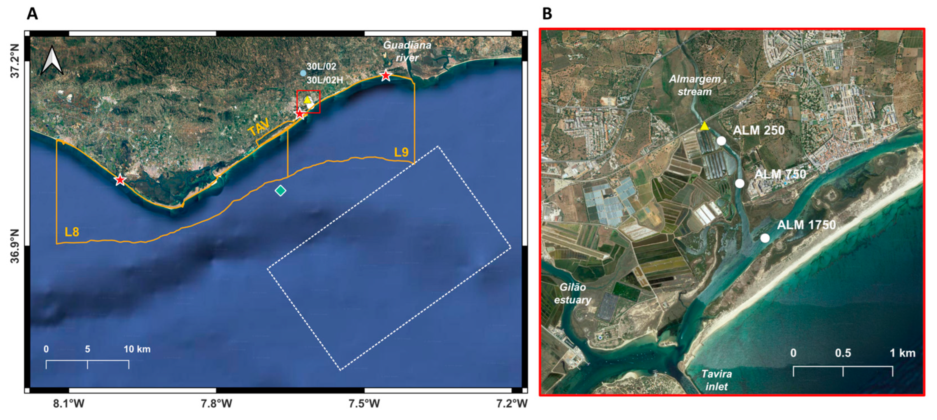
2.1. Study Area

Ria Formosa (RF) is a shallow coastal lagoon system (mean depth: 2 m) that extends along the south coast of Portugal, east and west of Cape Santa Maria (CSM), separated from the Atlantic Ocean by a barrier island system, but connected with the ocean through six inlets (Figure 1). RF is exposed to a semi-diurnal mesotidal regime, with a large fraction of the lagoon water volume (ca. 50–75%) exchanged with the ocean on a daily basis, and the water column is well-mixed, with no significant thermal or haline stratification [69]. However, water residence time is incremented, by more than two weeks, at inner lagoon areas [48,69]. The lagoon is mostly euryhaline, and the main permanent freshwater source is the Gilão River (mean annual discharge: 2.44 m³ s⁻¹; see [70]), which mainly affects the eastern sector of the lagoon [46,47,51]. The adjacent coastal area is affected by regular upwelling events, associated with strong westerly winds, which are more frequent during the spring–summer period, and the effects of which can extend up to ca. 6 km upstream of the lagoon inlets [43]. Despite its transitional nature, the RF lagoon has been classified under the Water Framework Directive as ‘sheltered coastal waters’ rather than ‘transitional waters’, due to the lack of salinity gradients [46]. This ecosystem is subjected to a Mediterranean climate, with hot, dry summers, and mild winters, and located in a region extremely vulnerable to climate change [49].

The study area, located in the eastern sector of the lagoon, is influenced by a natural freshwater source, the non-permanent Almargem stream (mean annual discharge: 0.11 m³ s⁻¹; see [70]), as well as exchange with the adjacent ocean through the Tavira inlet (Figure 1B). In addition, the study area is affected by one of the four main WWTPs discharging into the lagoon, the Almargem (ALM) WWTP, located on the left bank of the Almargem stream, next to the city of Tavira (see Figure 1B). Wastewater treatment includes primary physical treatment, followed by secondary biological treatment using activated sludge, and, finally, ultraviolet disinfection [71], and effluents are discharged into the Almargem stream (see Figure 1). In the study area, shellfish farming grounds, mainly for oysters (Crassostrea spp.) and clams (Ruditapes decussatus), are located west of the lower Gilão estuary.

2.2. Sampling Strategy

Water sampling was conducted along a longitudinal transect of the effluent dispersion from the ALM WWTP. Water physico-chemical variables, chlorophyll-a (Chl-a) concentration, and phytoplankton abundance and species composition were analyzed at three stations located at 250 m (ALM 250), 750 m (ALM 750), and 1750 m (ALM 1750) from the WWTP discharge point (Figure 1B). Water physico-chemical variables and chlorophyll-a concentration were also measured at three additional stations located at 500 m, 1000 m, and 1500 m from the ALM WWTP discharge point (Figure 1). The furthest station from the discharge point (ALM 1750) is located at ca. 1.5 km from the Tavira inlet. The three stations used in our study were selected based on previous studies in Ria Formosa, which reported the WWTP influence up to 750 m from the discharge points, followed by reference lagoon conditions for the furthest stations [30,47,56]. The distance between stations increased from those closer to the discharge point (500 m, ALM 250–ALM 750) to the outer stations (1000 m, ALM 750–ALM 1750) due to the occurrence of stronger water quality gradients in areas closer to the WWTP discharge points [30,47,56]. Thus, ALM 250 and ALM 750 were selected to represent different areas of influence of the WWTP, while ALM 1750 was selected as representative of the reference conditions for the outer lagoon main channels, capable of capturing the influence of adjacent coastal waters.

Sampling was undertaken monthly, over a 2-year period (September 2018–September 2020), during neap low tide. This tidal stage is referred to as representative of the poorest water quality in the RF lagoon, due to minimal tidal flushing and longer water residence time, allowing for a better evaluation of the effects of the WWTP effluent discharge (see [30]). No information is available for four months, due to logistic issues (January 2019, December 2019) or pandemic restrictions (February 2020, April 2020), thus under-representing these specific months and associated seasons. Water physico-chemical variables were measured in situ, and surface water samples (ca. 20–30 cm) were collected for the analysis of dissolved inorganic macro-nutrients, suspended solids, chlorophyll-a (Chl-a), and phytoplankton abundance and species composition.

2.3. Physico-Chemical, Meteorological, and Hydrographic Variables

Water temperature, salinity, dissolved oxygen, and pH were measured in situ using a YSI EXO2 multi-parameter probe (YSI Xylem Inc., Yellow Springs, OH, USA), with sensor specifications as described in [44]. For nutrient analysis, water samples were filtered through 0.45 µm membrane filters, and frozen at −20 °C until analysis. Ammonium, nitrate, nitrite, phosphate, and silicate concentrations were analyzed using spectrophotometric methods and calibration curves, with an Evolution 200 Thermo Scientific spectrophotometer (Thermo Fisher Scientific, Lisboa, Portugal), according to [72]. The Marine Nutrient Standards Kit (OSIL, Havant, UK) was used as reference material to ensure accuracy; precision ranged from ca. 1% for silicate, nitrite, and phosphate, to 2% for nitrate and ammonium. The detection limits were 0.1 µM for nitrate and ammonium, 0.05 µM for silicate, 0.03 µM for phosphate, and 0.02 µM for nitrite.

Daily rainfall precipitation (mm), measured at the closest land-based meteorological station to the study area (Station 2, Tavira; latitude: 37°06′53.9″; longitude: 07°39′20.7″), was extracted from Direção Regional de Agricultura e Pescas do Algarve (DRAPALG; Faro, Portugal; [73]). Water quality data for the Almargem stream, measured at Curral Boieiros water quality station (30L/02; Tavira, Portugal; see Figure 1A), was retrieved from the Portuguese Environmental Agency (APA) public database, when available [74]. No information on natural freshwater discharges into the eastern sector of the RF lagoon (Gilão River and Almargem stream) was available for the entire study period (September 2018–September 2020), thus limiting our evaluation of the relative importance of natural freshwater sources of nutrients. Daily Almargem stream discharge, measured at Curral de Boieiros hydrometric station (30L/02H; see Figure 1A) during the period July 2019–September 2020, was retrieved from the APA public database [74]. Further attempts to derive freshwater discharge for the entire study period, from area-specific empirical relationships between freshwater discharge, precipitation (hydrometric stations: Curral de Boieiros and Bodega; see [42]), and aquifer piezometric levels were unsuccessful. Thus, the Guadiana river discharge, measured daily at Pulo do Lobo hydrometric station (27L/01H; Mértola, Portugal), retrieved from the APA public database [74], was used as a proxy for the potential freshwater influence on the study area. Mean monthly data on the WWTP effluent discharge rate, total nitrogen load, and total phosphorus load during the study period were provided by the water supply company, Águas do Algarve (AdA; Faro, Portugal).

2.4. Oceanographic Setting at the Adjacent Coastal Area

Due to the lack of in situ observations, satellite remote sensing was used to characterize general oceanographic conditions in the adjacent coastal waters during the study period. This dataset complements the lagoon in situ measurements and was used to evaluate the potential stimulatory effects of upwelling events on phytoplankton, more expectable at the outer lagoon station. Level 3, 8-day composites of sea surface temperature (SST) data were retrieved from MODerate resolution Imaging Spectroradiometer, onboard the Aqua satellite (MODISA), available from NASA’s Oceancolor database [75]. SST data, at 4 km resolution, were limited to nighttime passes, to avoid diurnal solar heating effects [76], and to high quality data (AVHRR quality flags 6 and 7, and MODISA quality flag 0). SST data were averaged over a coastal area off Tavira inlet, covering domains east and west of the inlet (Figure 1A).

Upwelling intensity was estimated using a wind-based index, the cross-shore Ekman transport (CSET), which represents the magnitude of the offshore component of Ekman transport, comparable to the amount of water upwelled from the base of the Ekman layer [77]. Daily sea surface zonal (U) and meridional (V) wind fields, at 0.25° spatial resolution, were obtained from the Blended Sea Winds (BSW) dataset, available at NCEI-NOAA [78]. BSW is based on a combination of multiple scatterometers, standardized across platforms, resulting in high-quality ocean wind vectors [79]. CSET was computed for a single site, located ~11 km off the southern coast of Portugal (see Figure 1A), and values represent the average of a 0.75° × 0.75° box centred on the target location. As the southern Portuguese coast is zonally (west–east) oriented, CSET was estimated from the meridional component of the Ekman transport, induced by the zonal component of wind stress (for details see [80]). Negative values of the upwelling index indicate offshore Ekman transport and upwelling-favourable periods, whereas positive values represent onshore transport and downwelling-favourable periods.

2.5. Phytoplankton Data

2.5.1. Chlorophyll-a Concentration

Lagoon water samples for the analysis of Chl-a concentration, used as a proxy for total phytoplankton biomass, were filtered through GF/F glass fibre filters (nominal pore size = 0.7 µm) and frozen at −20 °C until analysis. Pigments were extracted, overnight, in cold 90% acetone and analyzed spectrophotometrically [81].

Satellite remote sensing was used to characterize Chl-a variability patterns in the adjacent coastal area, during the study period. Level 3, 8-day composites of surface Chl-a, at 4 km resolution, were retrieved from the European Space Agency (ESA)’s Ocean Colour Climate Change Initiative Group, OC-CCI [82]. This product combines information from multiple sensors (Sea-viewing Wide Field of View Sensor, MODISA, Medium Resolution Imaging Spectrometer, and Visible Infrared Imaging Radiometer Suite), allowing for increased spatial–temporal resolution [83]. Chl-a data were averaged over a coastal area off the Tavira inlet, covering domains east and west of the inlet (see Figure 1A), but avoiding optically complex near-shore water masses (see [84]). However, the use of remote sensing and a 4 km spatial resolution limited Chl-a analysis to the upper ocean surface, and precluded the observation of smaller-scale distribution patterns.

2.5.2. Phytoplankton Abundance and Composition

Water samples for phytoplankton abundance and species composition were preserved in Lugol’s solution immediately after collection, settled in sedimentation chambers (10 mL, 25 mL, and 50 mL), and observed using inversion microscopy (Zeiss Axio Observer A1; ZEISS, Lisboa, Portugal), according to [85]. The analysis comprised only plastidic cells, either strictly autotrophic or mixotrophic taxa, including microphytoplankton (>20 μm) and morphologically conspicuous nanophytoplankton (ca. 2–20 μm). A minimum of 400 cells were enumerated per sample and, assuming a random distribution of cells in the chamber, the counting precision was 10% [86]. Thus, this study only included the Utermöhl fraction of phytoplankton, which is an underestimate of total phytoplankton abundance, considering the high contribution of picophytoplankton in the RF lagoon (cyanobacteria and eukaryotes <2 μm; [54,63,64,65]).

Phytoplankton cells were identified to the lowest taxonomic level possible, typically genus and species, using morphological characteristics and taxonomic reference literature for marine [87,88,89] and freshwater phytoplankton [90,91]. Taxa difficult to discriminate at the species or genus level using inverted microscopy were aggregated into multi-taxa, broader taxonomic units (e.g., Pseudo-nitzschia seriata-group; athecate dinoflagellates; cryptophyceans; Heterocapsa/Azadinium; Pleurosigma/Gyrosigma; unidentified nanoflagellates), in some cases separated into different size classes. Taxonomic and nomenclatural information was updated according to the AlgaeBase database [92]. The classification of phytoplankton taxa as potentially harmful was based on the IOC-UNESCO Taxonomic Reference List of Harmful Micro Algae [93], AlgaeBase [92], and other references [5,89].

Our phytoplankton dataset was complemented with information on the abundance of two Pseudo-nitzschia groups (delicatissima and seriata) and Dynophysis spp., potentially toxigenic taxa frequently reported along the southern Portuguese coast, and responsible for the amnesic and diarrhetic shellfish poisoning syndromes (ASP and DSP, respectively) in humans [94]. Abundances of HAB taxa, measured approximately weekly, in classified lagoonal (‘Tavira’) and coastal (L8 and L9) shellfish production areas (see Figure 1A) were retrieved from the Portuguese Institute of the Sea and Atmosphere (IPMA) public database [95]. HAB abundances reported in this database as below the limit of detection (LOD) or not detected (ND) were considered as zero. The number of samples available for ASP- and DSP-producers were 99, 26, and 105 at Tavira, L8, and L9 shellfish production areas, respectively. For further details on the use of the IPMA database, see [94].

2.6. Data and Statistical Analysis

Basic assumptions for parametric analyses, including data normality and variance homogeneity, were tested using the Shapiro–Wilk and Fligner-Killeen tests, respectively, and non-parametric methods were used as appropriate. All statistical analyses were considered at a 0.05 significance level. Statistical analysis and data visualization were performed using R version 4.0.3 [96] and specific R packages.

2.6.1. Univariate Analysis of Phytoplankton and Environmental Data

Different phytoplankton groups, identified to the lowest taxonomic level possible but at different taxonomic levels, were treated as operational taxonomic units (OTUs). All OTUs were later binned into broader taxonomic groups, including functional types (planktonic diatoms and benthic diatoms) or specific phyla. For each sample, the phytoplankton assemblage structure was characterized using several univariate descriptors, including abundance (expressed as cells per litre), and alpha diversity metrics. These included the observed OTU richness, estimated OTU richness based on Chao1 diversity estimator [97], Hulburt’s dominance index (see [9]), Shannon–Wiener diversity index, and Pielou evenness index [98], and were calculated using the R packages vegan (v2.6.2; [99]) and BiodiversityR (v2.14.4; [100]).

Differences in phytoplankton diversity metrics between lagoon stations and seasons were tested using the KruskalWallis test, a one-way analysis of variance by ranks, followed by Dunn’s post-hoc test. Differences in physico-chemical variables, Chl-a concentration, and phytoplankton abundances between lagoon sampling stations or shellfish production areas were tested using Durbin’s rank test, a Friedman-type test for balanced incomplete block designs, followed by multiple pairwise comparisons of rank sums using the post-hoc Durbin test [101].

2.6.2. Multivariate Analysis of Phytoplankton and Environmental Data

The multivariate analysis included the use of two ordination techniques, and an exploratory and an interpretative technique. All physico-chemical environmental data (water temperature, salinity, dissolved oxygen, pH, suspended solids, and ammonium, nitrate, nitrite, phosphate, and silicate) were converted to z-scores, i.e., standardized to zero mean and unit variance, to eliminate scale dependence in subsequent analyses (e.g., [102]). For phytoplankton, OTUs detected in less than 5% of the samples were excluded from all multivariate analyses, to reduce the influence of rare taxa (e.g., [103]), and the Bray–Curtis dissimilarity measure was used to compute phytoplankton distance matrices. Multivariate analyses were computed using the following R packages: vegan (v2.6.2; [99]), goeveg (v0.5.1; [104]), pairwiseAdonis (v0.4; [105]), and indicspecies (v1.7.12; [106]).

Non-metric multidimensional scaling (NMDS), an exploratory unconstrained ordination analysis, was used to identify spatial–temporal patterns in phytoplankton assemblage structure. NMDS is commonly considered as the most robust unconstrained ordination method in community ecology, showing a good performance on non-normal discontinuous data [107,108]. Phytoplankton abundance data were log(x + 1) transformed prior to analysis, to account for non-normal data distribution and reduce the disproportionate influence of dominant OTUs (e.g., [103]). The analyses were run several times, to obtain the best NMDS ordination. The goodness of fit of NMDS ordinations was assessed using the stress value, and the lowest stress value possible was selected, considering a 0.2 threshold value [103,109]. The number of NMDS axes was defined using stress plot analyses, and a Shepard diagram was used to assess the representativeness of the best ordination.

Differences in the structure of phytoplankton assemblages between study sites and seasons were tested using permutational multivariate analysis of variance (PERMANOVA; [110]), based on a Bray–Curtis similarity matrix. Study site (3 levels) and season (4 levels) were used as fixed factors. A conventional division of seasons was considered: winter (January–March), spring (April–June), summer (July–September), and autumn (October–December). Differences between seasons, randomly nested in site, were also tested. Significant effects were tested using post hoc pairwise comparisons with PERMANOVA F-statistic and 999 permutations, using the R pairwiseAdonis function ‘pairwise.adonis’. Similarity Percentage Analysis (SIMPER) was used to assess the percentage contribution of each OTU to the average dissimilarity between factor levels [111], based on the R vegan function ‘simper’, allowing for the identification of potentially discriminating OTUs.

Indicator species analysis was also used to identify potential indicator OTUs that could typify specific sampling stations or seasons (e.g., [10,41]). This analysis was based on the Indicator Value (IV) index [106,112], computed by the R indicspecies function ‘multipatt’. The higher the mean abundance and relative frequency of occurrence of each OTU, the higher the IV. OTUs with IV >30% and p-value < 0.05 were considered as reliable indicators [10]. The significance of the indicator values for each OTU was tested using a Monte Carlo permutation test, with 999 random permutations. The classification of OTUs into generalists and specialists, at the station or season level, was based on the criteria defined by [41,113]. OTUs with IV >30%, similar for all stations or seasons were considered generalists. OTUs with IV >30% for at least one station or season, but statistically different between them, were considered specialists. When permutation-based p-values were not available, OTUs with IV >30% were not classified as indicators [106].

The R vegan function ‘envfit’ was applied to determine which individual environmental variables best explained spatial–temporal patterns in phytoplankton assemblage structure detected in the NMDS ordination. The variance explained (r²) by regressing each environmental variable onto the phytoplankton ordination axis and its p-values were used to assess the significance of these relationships [99]. Biota-Environment Stepwise Analysis (BIOENV) was also used to determine which combination of environmental variables best explained the phytoplankton assemblage patterns, based on the R vegan function ‘bioenv’ [114]). Significance was measured by the value of the Spearman correlation coefficient (r_S), and associated p-value, using the Mantel test (R vegan function ‘mantel’).

In addition, Canonical Correspondence Analysis (CCA), an interpretative constrained ordination analysis, was used to assess the relationships between abiotic environmental variables and specific phytoplankton OTUs. CCA assumes a unimodal relationship between species and environmental variables, and allows for the study of long environmental gradients, creating the best synthetic environmental gradients that maximally separate species niches (see reviews [107,115]). Abundance data of phytoplankton OTUs detected in more than 95% of the samples were square root transformed, prior to analysis. A stepwise procedure, starting with a model including all environmental variables, was used to select only those that significantly contributed to the CCA model. Collinear environmental variables, with variance inflation factors (VIF) higher than 10, were excluded using the R ‘vif.cca’ function. Monte Carlo permutation tests (999 permutations) were used to assess the significance of each variable and CCA axis [116]. The location of each species in respect to the environmental vectors is usually considered as indicative of the niche optima conditions. However, this interpretation should be considered cautiously due to the underlying assumptions (species distribution under environmental control, unimodal distribution for each variable, implying relatively long gradients; see [108]).

3. Results

3.1. Abiotic Environmental Setting

This study evaluated a series of abiotic environmental variables representative of the external natural and anthropogenic forcings acting on the RF lagoon, including meteorological, hydrological (precipitation, Guadiana River discharge, WWTP effluent discharge) and oceanographic variables (SST and CSET), as well as the physico-chemical conditions of the lagoon water. The basic statistical information for these variables (e.g., mean, standard deviation, minimum and maximum values) and differences between stations are summarised in the Supplementary Materials (Tables S1 and S2).

3.1.1. External Forcings: Meteorological, Hydrological, and Oceanographic Variables

During the study period (September 2018–September 2020), daily rainfall precipitation averaged 0.9 ± 3.3 mm, with high precipitation events (20–30 mm) occurring during the autumn–winter period (e.g., November 2018, December 2019) and spring 2020 (Figure S1). Higher Guadiana River discharge was generally associated with stronger rainfall events, namely in December 2019 and in January and April 2020, indicating a potentially greater influence of natural freshwater sources in the study area (Figure S1). The daily discharge of the Almargem stream, measured 4.7 km upstream of the WWTP discharge point only during the period July 2019–September 2020, averaged 0.00025 m³ s⁻¹ (i.e., 21.5 m³ d⁻¹; see Table S1), and was above zero on only three days (15–17 April 2020, 0.01–0.05 m³ s⁻¹, 3-day period average: 3456 m³ d⁻¹). The statistical information (mean ± SD) of the water quality of the Almargem stream, available only for the period 1994–2018 (n = 28–78), were the following: dissolved oxygen saturation: 95.7 ± 12.74%; nitrate: 37.8 ± 43.93 μM; ammonium: 1.44 ± 1.78 μM; phosphate: 0.38 ± 0.24 μM; and total suspended solids: 10.36 ± 43.84 mg L⁻¹.

The effluent discharge rate of the ALM WWTP averaged ca. 4093 m³ day⁻¹, with a mean total nitrogen load two times higher than the total phosphorus load (Table S1). The mean effluent discharge was ca. 2-fold lower than the historical discharge of the Almargem stream (9863 m³ day⁻¹, [117]), but almost 200 times higher than the mean stream discharge measured at Curral de Boieiros hydrometric station during the period July 2019–September 2020 (ca. 22 m³ day⁻¹).

Over the adjacent coastal waters, the SST showed minimum values during December-February, and the maxima during July–September (Figure S2A). The upwelling intensity, estimated using the wind-based index CSET, averaged −97.4 ± 962.4 m³ s⁻¹ km⁻¹ coastline. Upwelling-favourable conditions were detected more regularly during the spring–summer period, namely, in 2019, but were also observed during other periods, such as January 2019 and October–December 2019 (Table S1 and Figure S2A).

3.1.2. Physico-Chemical Conditions in the Ria Formosa Lagoon

Water temperature, salinity, dissolved oxygen, and total suspended solids averaged 21.4 °C, 31.9, 9.4 mg O₂ L⁻¹ (129.6% O₂ saturation), and 10.3 mg L⁻¹, respectively (Table S2). The mean concentrations of dissolved macronutrients were as follows: 6.2 μM N-NO₃⁻ (nitrate), 14.4 μM N-NH₄⁺ (ammonium), 6.6 μM P-PO₄³⁻ (phosphate), and 22.5 μM Si-SiO₄⁴⁻ (silicate) (Table S2). Salinity progressively increased along the longitudinal transect from the WWTP discharge point, while nutrient concentrations decreased. Compared to other stations, the mean concentration of dissolved oxygen was higher at ALM 250, and total suspended solids at ALM 250 and ALM 750 (see Table S2).

Most physico-chemical variables showed clear intra-annual variability patterns, which were stronger at stations closer to the WWTP discharge point (Figure 2). Water temperature and salinity exhibited lower values in winter and higher values from summer to late autumn, at all stations and for both years (Figure 2A,B). Atypical salinity minima values (ca. 9 and 20 at ALM 250 and ALM 750, respectively) were detected in spring 2020, during a period of high rainfall and freshwater discharge, coinciding with the maxima silicate concentrations for these two stations (ca. 65 μM and 100 μM; Figure 2A,H). Dissolved oxygen saturation showed higher values during summer (up to ca. 300%), namely at ALM 250 and ALM 750 (Figure 2C). Intra-annual variability patterns of the nutrient concentrations differed between the sampling stations and years (Figure 2E–H). At ALM 250 and ALM 750, the ammonium, nitrate, and phosphate concentrations were generally higher in autumn 2018 (after intense rainfall period; Figure S1), and late summer, namely, during 2019 (Figure 2E–G). At ALM 1750, except for phosphate, nutrients mostly showed higher concentrations between winter and early spring, with steep declines thereafter and minima in summer. Episodes of high ammonium and nitrate concentrations were also detected in August 2019 and November 2019, respectively (Figure 2E–H).

3.2. Phytoplankton Assemblage Structure

The basic statistical information on the phytoplankton metrics (Chl-a, abundance, and diversity) for the three sampling stations is summarized in

Table 1. Statistical information, including mean, standard deviation (SD), minimum (Min) and maximum (Max) values, number of observations (N), for chlorophyll-a concentration, the abundance of specific phytoplankton operational taxonomic units (OTUs), and diversity metrics, for the three lagoon stations (ALM 250, ALM 750, and ALM 1750). The mean annual relative contribution (%) of different phytoplankton groups to ‘total’ abundance, at each station, is also included (in brackets, after mean ± SD). Significant differences between stations (DbS) are also included. Asterisk symbols: *, **, and *** indicate p-values < 0.05, <0.01, and <0.001, respectively. bd: below detection limit; na: not available; ns: not significant.

Variable	Station (ALM)	Mean ± SD [% Contr.]	Min–Max	N	DbS
Chlorophyll-a concentration and phytoplankton abundance
Chlorophyll-a (µg L−1)	250	8.5 ± 25.4	0.5–115.2	20	250 > 1750 ** and 750 > 1750 *
	750	9.0 ± 28.6	0.4–126.5	19
	1750	1.5 ± 1.1	0.2–4.5	19
Total Abundance (×103 cells L−1)	250	8.131 ± 21.826	0.147–98.733	20	ns
	750	4.767 ± 8.805	0.132–38.151	19
	1750	2.148 ± 2.180	0.130–7.600	19
Planktonic Diatoms (×103 cells L−1)	250	5.052 ± 17.522 [73.7]	bd–78.432	20	ns
	750	2.626 ± 7.718 [63.6]	bd–33.580	19
	1750	1.19 ± 1.87 [60.4]	bd–5.922	19
Pseudo-nitzschia spp. (×103 cells L−1)	250	0.011 ± 0.026 [0.2]	bd–0.089	20	250 < 1750 *** and 750 < 1750 * and 250 < 750 *
	750	0.056 ± 0.182 [1.3]	bd–0.801	19
	1750	0.173 ± 0.416 [7.7]	bd–1.782	19
Cryptophyceans (×103 cells L−1)	250	1.092 ± 1.281 [16.8]	0.069–4.566	20	ns
	750	0.978 ± 1.033 [24.5]	0.032–4.04	19
	1750	0.579 ± 0.678 [25.1]	0.016–3.049	19
Plastidic Dinoflagellates (×103 cells L−1)	250	0.184 ± 0.286 [2.7]	0.008–1.132	20	ns
	750	0.152 ± 0.254 [3.7]	0.004–0.981	19
	1750	0.057 ± 0.090 [2.7]	0.0002–0.376	19
Kryptoperidinium foliaceum (×103 cells L−1)	250	0.075 ± 0.136 [1.1]	bd–0.410	20	250 > 1750 *** and 750 > 1750 ***
	750	0.089 ± 0.187 [2.1]	bd–0.711	19
	1750	0.0002 ± 0.001 [0.01]	bd–0.005	19
Benthic Diatoms (×103 cells L−1)	250	0.18 ± 0.26 [2.7]	0.003–0.92	20	ns
	750	0.12 ± 0.15 [2.8]	0.009–0.39	19
	1750	0.06 ± 0.07 [3.5]	0.002–0.260	19
Cyanobacteria (×103 cells L−1)	250	0.197 ± 0.24 [2.8]	bd–0.8190	20	ns
	750	0.081 ± 0.1384 [1.9]	bd–0.5341	19
	1750	0.0078 ± 0.0167 [0.5]	bd–0.0585	19
Phytoplankton diversity metrics
Estimated species richness (Observed Species richness)	250	136.2 (93)	na	21	na
	750	132.7 (90)	na	20
	1750	152.6 (120)	na	21
Average observed species richness	250	19.9 ± 6.4	8–34	21	250 < 1750 ** and 750 < 1750 *
	750	20.7 ± 6.1	10–32	20
	1750	27.1 ± 8.9	11–41	21
Species dominance (Hulburt index)	250	69.3 ± 14.7	39.9–95.5	21	ns
	750	66.2 ± 13.7	40.1–92.3	20
	1750	63.6 ± 14.0	37.3–90.3	21
Species diversity (Shannon–Wiener index)	250	1.6 ± 0.4	0.6–2.2	21	ns
	750	1.6 ± 0.4	0.6–24	20
	1750	1.7 ± 0.4	0.8–2.5	21
Species evenness (Pielou index)	250	0.5 ± 0.2	0.2–0.8	21	ns
	750	0.5 ± 0.1	0.2–0.8	20
	1750	0.5 ± 0.1	0.2–0.8	21

. Considering only morphologically distinct nanoplankton and microplankton cells, a total of 147 phytoplankton OTUs were observed (including species and broader taxonomic units), of which 57 OTUs were present in all stations (see Table S3). A total of 47 OTUs (32%) were present at only one station, 10 OTUs at ALM 250, 7 OTUs at ALM 750, and 30 OTUs at ALM 1750. OTUs included 27 benthic taxa (dominated by diatoms), 11 OTUs generally associated with freshwater systems (dominated by chlorophytes), and several potentially harmful taxa (e.g., Dinophysis acuminata complex, Pseudo-nitzschia spp., Kryptoperidinium foliaceum, Heterosigma akashiwo) (see Table S3).

Overall, the 147 OTUs detected were assigned to the following nine phyla: 68 Heterokontophyta (including 67 diatoms and 1 silicoflagellate), 52 Dinoflagellata, 10 Chlorophyta, 7 Cyanobacteriota, 3 Euglenophyta, 3 Ochrophyta, 2 Cryptista, 1 Charophyta, and 1 Haptophyta. Diatoms and dinoflagellates thus represented ca. 46% and 34% of the total OTU richness (see Table S3). Considering each sampling station individually, the observed OTU richness (90–120, see Table S3) was higher at ALM 1750, and lower than the estimated richness (Chao1: 132.7–152.6; see Table 1).

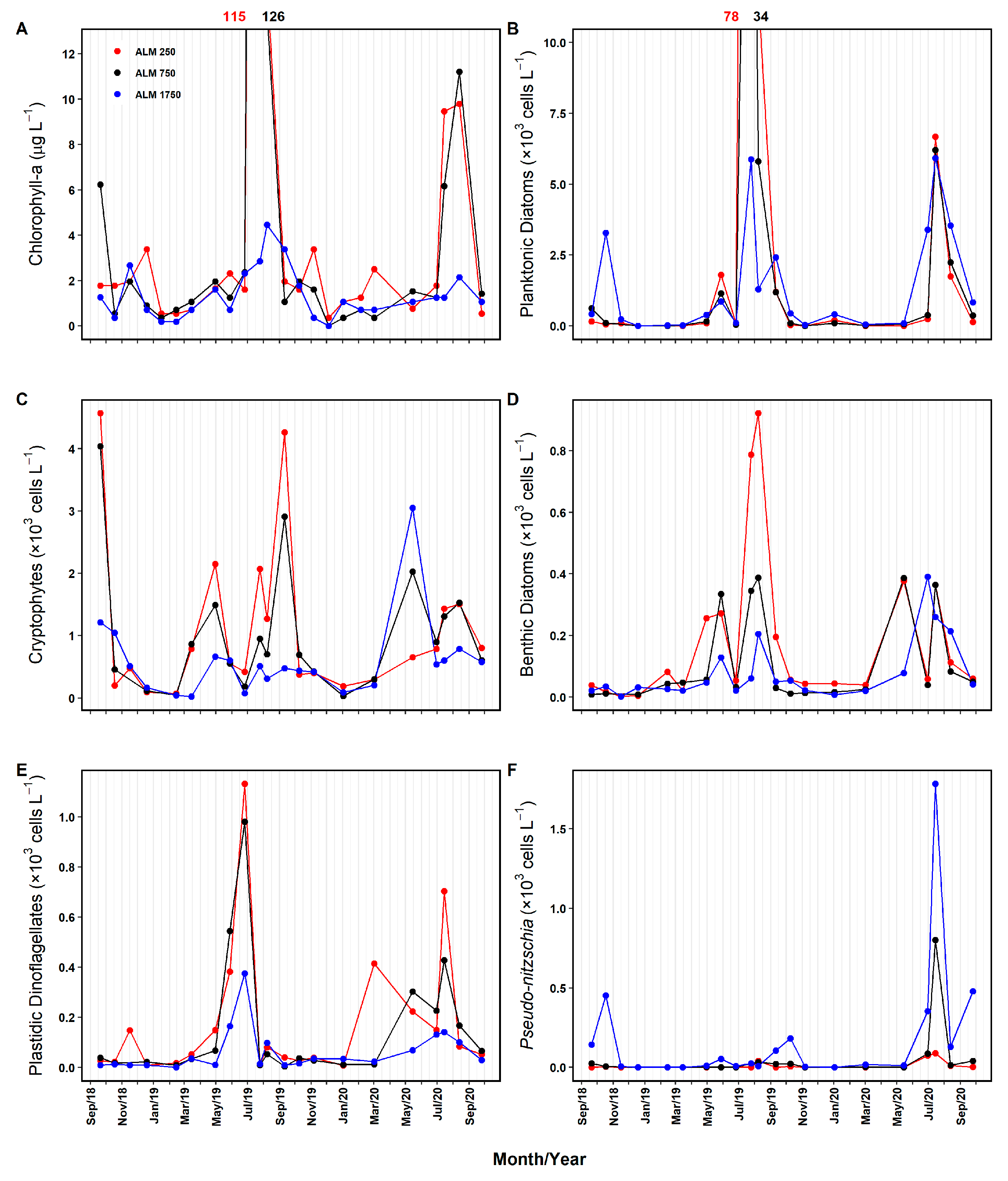
3.2.1. Phytoplankton Biomass, Abundance, and Diversity

Chl-a concentration (0.2–126.5 μg L⁻¹), used as a proxy for the phytoplankton biomass, was, on average, ca. 6-fold lower at ALM 1750 compared to other stations (Table 1). In terms of abundance, the phytoplankton assemblages were globally dominated by planktonic diatoms (2976.5 ± 10,801.6 cells L⁻¹) and cryptophyceans (899.8 ± 1011.3 cells L⁻¹), with minor contributions from plastidic dinoflagellates (131.5 ± 222.8 cells L⁻¹), benthic diatoms (126.5 ± 181.3 cells L⁻¹), and cyanobacteria (92.7 ± 173.9 cells L⁻¹). Considering each sampling station individually, planktonic diatoms, cryptophyceans, plastidic dinoflagellates, benthic diatoms, and cyanobacteria represented, on average, 60–74%, 17–25%, 3–4%, 3–4%, and 1–3% of ‘total’ phytoplankton abundance, respectively (Table 1). Although the mean abundances of the whole phytoplankton assemblage or the main functional groups decreased from ALM 250 to ALM 1750, no significant differences were detected between the stations. However, differences between the stations were observed for specific groups, including potentially harmful taxa. Kryptoperidinium foliaceum was more abundant in the innermost lagoon stations, closer to the WWTP discharge point (ALM 250 and ALM 750, p < 0.001). For Pseudo-nitzschia spp., the abundance increased progressively from ALM 250 to ALM 1750, closer to the Tavira inlet (p < 0.05; Table 1). For the latter (ASP-producers), significantly higher abundances were observed in the lagoonal (‘Tavira’, p < 0.001) and coastal shellfish production areas (L8 and L9, p < 0.001) in respect to ALM stations (see Figure S3). Higher abundances of Dinophysis spp. (DSP producer) were also observed in coastal shellfish production areas in respect to the lagoonal stations (p < 0.001; see Figure S3).

In terms of the diversity metrics that aggregate abundance and composition, the phytoplankton dominance (δ), diversity (H′), and evenness (J′) ranged between 37.3 and 95.5%, 0.6–2.5, and 0.2–0.8, respectively. No differences between stations were detected for the diversity metrics, except for the mean OTU richness, which was higher at ALM 1750 compared to the other stations (p < 0.05; Table 1).

Regarding the temporal variability, Chl-a concentration showed similar intra-annual patterns at all stations, with lower values detected during the autumn–winter period, and higher values during summer, for both years. In July 2019, the notoriously high Chl-a values detected at the ALM 250 and ALM 750 stations (115.2–126.5 μg L⁻¹; see Figure 3A) coincided with extreme silicate minima (0.4–0.5 μM) and oxygen saturation maxima (300.0–363.9%; Figure 2C,H). In the adjacent coastal region, strongly connected with ALM 1750, the Chl-a increases started earlier (November) for both years, reaching peak values during winter, which were anticipated and more intense in 2020 (Figure S2B), after strong autumn upwelling activity (Figure S2A). Relative increases were also observed in late spring/summer, which were more sustained in 2019, under a stronger, more persistent summer upwelling intensity (see Figure S2A,B).

Planktonic diatoms paralleled the Chl-a variability patterns at all stations, with the maxima abundance in summer, namely, in July 2019, at the stations ALM 250 and ALM 750 (Figure 3B). The other major functional groups, cryptophyceans, benthic diatoms, and plastidic dinoflagellates, and the potentially harmful Pseudo-nitzschia spp. generally showed higher abundances during the spring–summer period, for both years (Figure 3C,D), but the increase in the cryptophyceans abundance started in spring, earlier than that of diatoms (Figure 3B,C). Considering the phytoplankton diversity metrics, no differences in the average OTU richness, diversity, and dominance indices were detected between seasons. However, the evenness index was lower in summer compared to the other seasons (p < 0.05; see Table S4).

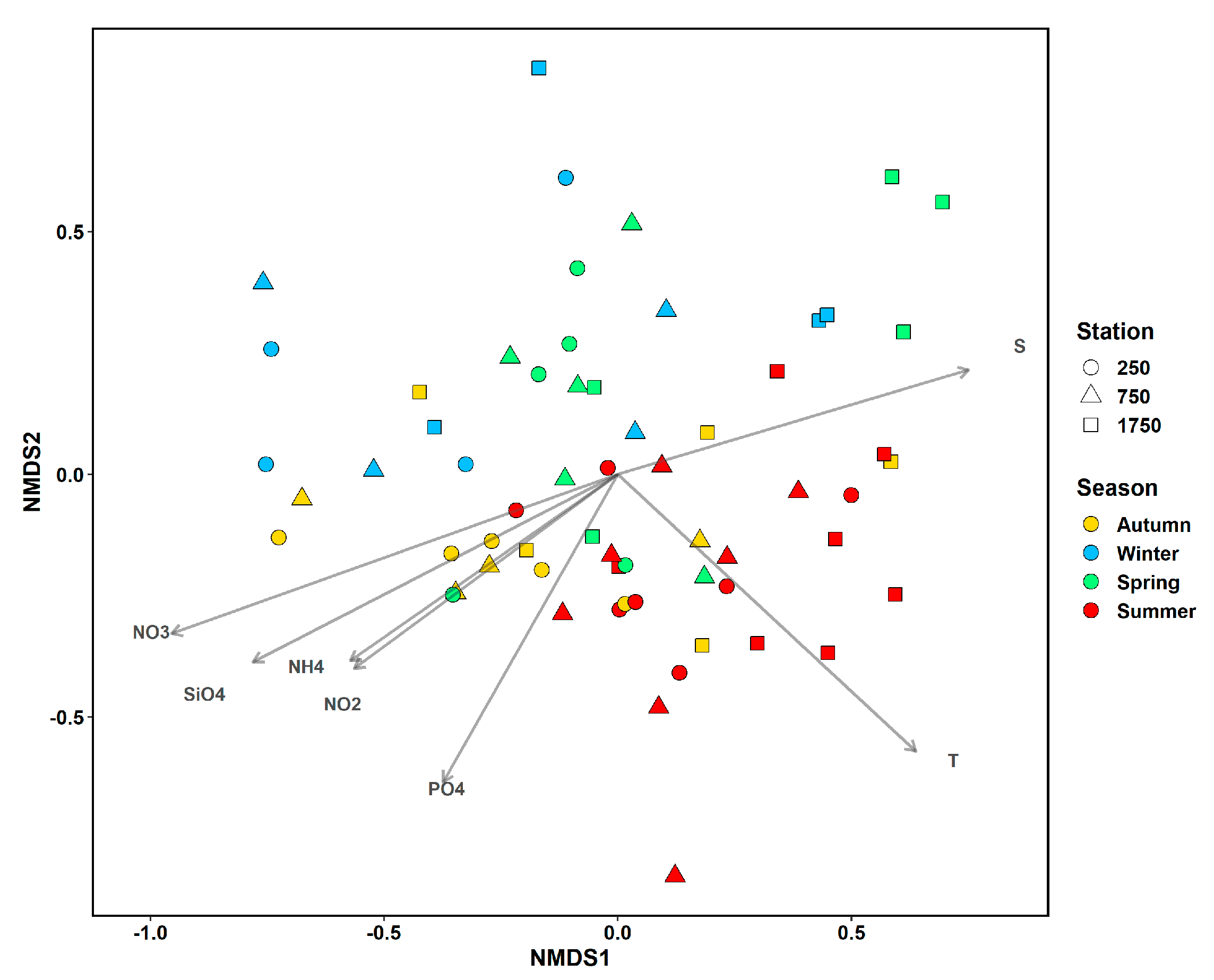
3.2.2. Phytoplankton Assemblage Structure and Main Taxa Contributing to Dissimilarity

The distance matrices used to explore the spatial–temporal patterns in the phytoplankton assemblage structure were composed of 62 samples (3 sampling sites × 21 sampling dates) and 81 OTUs (detected in more than 5% of the samples, out of the 147 OTUs). The NMDS analyses resulted in a four-dimensional ordination with a stress value of 0.14, and the ordination plot arranged the samples according to the site and season (Figure 4). The location of samples from the stations ALM 250 and ALM 1750 were mostly concentrated in the left and right plot areas, respectively. Furthermore, the summer samples were mostly plotted in the lower right plot area, and the winter samples in the upper plot area (Figure 4). These patterns were further supported by the PERMANOVA analysis, which revealed highly significant differences in the structure of the phytoplankton assemblages between the stations and seasons (p < 0.001). Pairwise comparisons showed significant differences between ALM 1750 and the other stations, stronger for the station closest to the WWTP discharge point (ALM 250, p < 0.001), and similar phytoplankton assemblage structures at the two innermost stations, ALM 250 and ALM 750 (Table S5). Significant differences were also detected between all seasons, being weaker between autumn and winter (p < 0.01, Table S5).

SIMPER analysis ranked the phytoplankton OTUs according to their contribution to the overall dissimilarity in the assemblage structure between stations and seasons. In terms of the spatial variability, the average dissimilarity between ALM 1750 and the other two stations varied between 58 and 59% (Tables S6 and S7) and was explained by a large number of discriminating OTUs with low individual contributions to the overall dissimilarity (≤5%). A total of 27 OTUs accounted for 70% of the cumulative dissimilarity, all of which were present at all stations but at different abundances (Tables S6 and S7). The most influential discriminating OTUs (individual contributions >3%) included Chaetoceros spp., Pseudo-nitzschia delicatissima group, unidentified chlorophytes (more abundant at station ALM 1750), Thalassiosira sp. (more abundant at station ALM 750), Kryptoperidinium foliaceum, cryptophyceans <10 μm, unidentified Oscillatoriales, Eutreptiella sp. (more abundant at stations ALM 250 and ALM 750), and benthic pennate diatoms <10 μm (more abundant at station ALM 250). Considering seasonal variability (54–66% dissimilarity), higher dissimilarities were detected for winter compared to spring (61%) and summer (66%) assemblages (Tables S8–S13). A total of 31 OTUs accounted for 70% of the cumulative dissimilarity. The most influential OTUs included the nine OTUs referred to above, plus unidentified Gymnodiniales <20 μm, pennate diatoms >10 μm, unidentified coccolithophores, Cylindrotheca closterium, Sundstroemia setigera/S. pungens, Cyclotella sp. and Skeletonema sp. (Tables S8–S13). Most of the OTUs were generally more abundant during summer, in respect with the other seasons, but some of the OTUs showed higher abundances during other seasons (Tables S8–S13).

Indicator species analysis, applied to 81 phytoplankton OTUs, highlighted a total of 29 OTUs with IV >30%, potentially of value as indicators. These included only one generalist OTU, cryptophyceans <10 μm (IV >30% for all stations), and 19 specialist OTUs, with 8 season specialists and 11 station specialists (

Table 2. List of phytoplankton operational taxonomic units (OTUs), and corresponding taxonomic divisions, that emerged as indicators of the structure of phytoplankton assemblages in the lagoon, in the whole study area (generalists) or at specific sampling stations (specialists). Sampling stations: ALM 250, ALM 750, and ALM 1750. Indicator OTUs, with indicator value index (IV) above 30%, are listed in alphabetical order. Generalist (p-value > 0.05) and specialist OTU indicators (p-value < 0.05) are highlighted in bold. Asterisk symbols * and ** indicate p-value < 0.05 and ≤0.01, respectively. ns: not significant. Symbols next to each taxa represent different phytoplankton groups, including diatoms or specific phyla: ▼—Chlorophyta; +—Cryptista; □—Cyanobacteriota; ∆—Diatoms; ○—Dinoflagellata; ˆ—Euglenophyta; ●—Haptophyta.

Phytoplankton OTUs	IV (%)			p-Val.
	250	750	1750
Chaetoceros spp. ∆	14.2	22.5	36.8
Unidentified Chlorophyte 1 ▼	27.9	25.7	33.6
Unidentified Coccolithophores ●	31.6	29.1	17.8
Unidentified Cryptophyceae >10 μm +	28.3	33.4	31.8
Unidentified Cryptophyceae <10 μm +	33.3	31.4	30.4	ns
Dinophysis acuminata complex ○	0	0	38.1	**
Eutreptiella spp. ˆ	25.8	34.3	15.7
Unidentified Gymnodiniales <20 μm ○	36.6	25.6	19.4
Heterocapsa spp. ○	5.2	2.0	40.2	*
Kryptoperidinium foliaceum ○	47.4	41.1	0.5	**
Unidentified Oscillatoriales □	31.0	22.4	2.4	**
Unidentified Pennales >10 μm ∆	34.9	30.4	23.6
Prorocentrum cf. scutellum  ○	0.1	0	37.1	**
Prorocentrum micans ○	0.8	0.2	52.4	**
Prorocentrum spp. ○	0.1	0	37.7	**
Prorocentrum triestinum ○	0	0.02	33.2	**
Pseudo-nitzschia delicatissima group ∆	7.8	21.1	35.3
Pseudo-nitzschia seriata group ∆	0.9	6.9	48.1	**
Scrippsiella spp. ○	1.7	2.2	55.8	**
Tripos fusus ○	0.1	0	37.2	**

and

Table 3. List of phytoplankton operational taxonomic units (OTUs), and corresponding taxonomic divisions, that emerged as indicators of the structure of phytoplankton assemblages in the lagoon, at specific seasons. Indicator OTUs (all specialists), with indicator value index (IV) above 30% (p-value < 0.05), are listed in alphabetical order, and highlighted in bold. Asterisk symbols * and ** indicate p-value < 0.05 and ≤0.01, respectively. ns: not significant. Symbols next to each taxa represent different phytoplankton groups, including diatoms or specific phyla: ●—Charophyta; ▼—Chlorophyta; +—Cryptista; ∆—Diatoms; ○—Dinoflagellata; and ˆ—Euglenophyta.

Phytoplankton OTUs	IV (%)				p-Val.
	Autumn	Winter	Spring	Summer
Akashiwo cf. sanguinea ○	33.1	0	0	1.0	**
Chaetoceros spp. ∆	6.5	3.6	30.4	39.1	**
Unidentified Chlorophyte 1 ▼	21.9	6.2	20.8	41.8
Closterium sp. ●	0	41.7	0	0	**
Unidentified Cryptophyceae <10 μm +	21.1	13.5	29.5	31.6
Cylindrotheca closterium ∆	7.8	21.4	18.4	36.1
Eutreptiella spp. ˆ	37.1	2.9	14.4	27.8	**
Unidentified Gymnodiniales <20 μm ○	13.9	6.7	38.4	26.3
Kryptoperidinium foliaceum ○	7.9	13.9	45.7	8.7
Navicula spp. ∆	1.1	9.2	30.3	5.6	ns
Unidentified Pennales >10 μm ∆	11.2	16.8	35.2	27.6
Unidentified Pennales <10 μm ∆	2.9	9.3	15.7	40.8	**
Pseudo-nitzschia delicatissima group ∆	14.1	1.4	7.0	48.7	*
Sundstroemia setigera/S. pungens ∆	1.0	0.2	0	65.8	**
Thalassiosira sp. ∆	0.2	1.7	1.1	50.2	**
Unidentified thecate dinoflagellates >20 μm ○	0.4	2.3	30.5	11.2	ns

). Most specialists (13 OTUs) were present at all stations but at different abundances (Table S3). The station specialists included unidentified Oscillatoriales (ALM 250), Kryptoperidinium foliaceum (ALM 250 and ALM 750), and a group of eight dinoflagellates and one diatom for ALM 1750. At the latter station, the specialist OTUs included Scrippsiella spp., Prorocentrum micans, Heterocapsa spp., Dinophysis acuminata complex, Prorocentrum spp., Tripos fusus, Prorocentrum scutellum, Prorocentrum triestinum, and Pseudo-nitzschia seriata complex (Table 2).

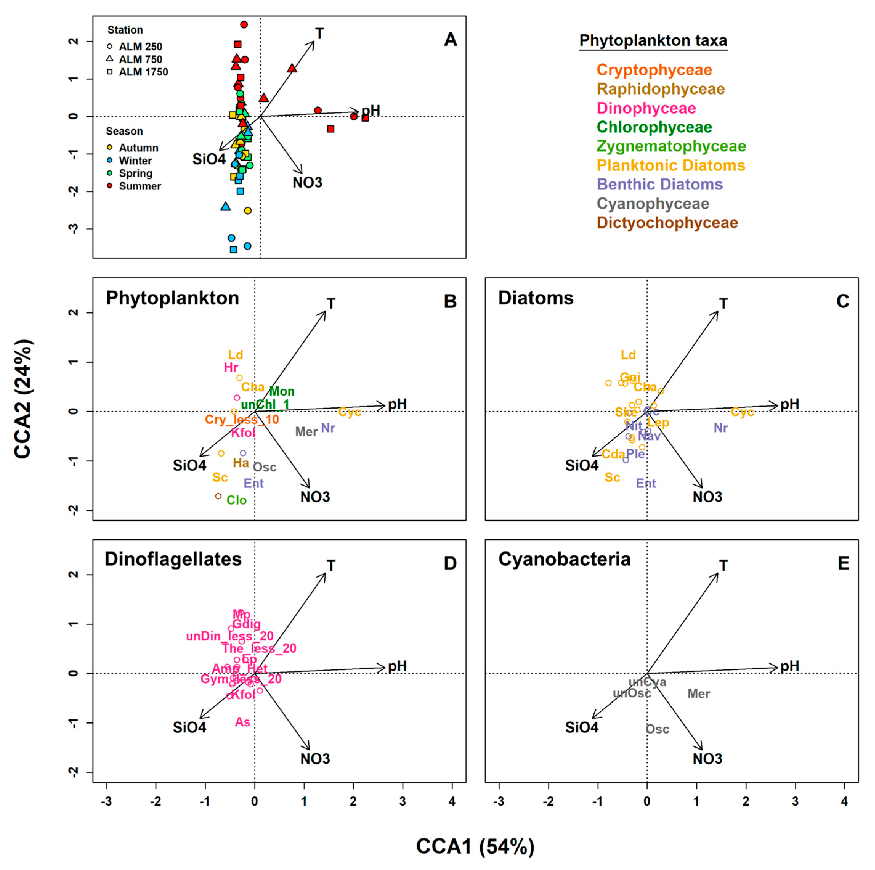
3.3. Linkages between Phytoplankton Assemblage Structure and Abiotic Environmental Variables

The spatial–temporal patterns in the structure of phytoplankton assemblages during our study, identified by NMDS analysis, were significantly correlated with changes in some abiotic environmental variables. The R ‘envfit’ function identified seven highly significant variables, superimposed on the NMDS ordination plot (see Figure 4): water temperature (p < 0.01), salinity (p < 0.001), and concentrations of nitrate, silicate, phosphate, ammonium, and nitrite (p < 0.01). According to the BIOENV analysis, water temperature, the most significant variable identified by the ‘envfit’ function, and nitrate concentration represented the combination of abiotic environmental variables that best explained the changes in the phytoplankton assemblage structure (r_S = 0.38, p = 0.01).

CCA analysis showed that four abiotic environmental variables, the water temperature, pH, and nitrate and silicate concentrations, significantly explained the total variance in the phytoplankton assemblage structure (23% of total variance explained, F = 4.2, and p = 0.001; Figure 5). Except for pH, these also emerged as influential abiotic variables in the ‘envfit’ and BIOENV analysis. The eigenvalues for the first two canonical axes (CCA 1: 0.379; and CCA 2: 0.165) explained 78% of the constrained variance in the phytoplankton structure (phytoplankton–environment relationship) with the CCA 1 and CCA 2 accounting for 54% and 24%, respectively. The first axis was positively correlated with pH (canonical coefficient, r = 0.71), nitrate (r = 0.41), and temperature (r = 0.17), and negatively with silicate (r = −0.24). The second axis was positively related with temperature (r = 1.00), and negatively related with silicate (r = −0.47) and nitrate (r = −0.29). Overall, the CCA analysis extracted two synthetic environmental gradients: a strong gradient, characterized by increases in pH, nitrate, and temperature, with concomitant decreases in silicate, and a secondary gradient characterized by increases in temperature with concurrent decreases in the silicate and nitrate concentrations. The projection of the samples onto the CCA plot showed that seasonal changes in the phytoplankton assemblages occurred, predominantly, along the second environmental gradient (summer and winter located at the lower and upper plot areas, respectively), while changes during summer were additionally associated with the first environmental gradient (see Figure 5A).

The projection of the phytoplankton taxa onto the first and second CCA axes revealed the distribution of the major OTUs along these environmental gradients. OTUs near (distant) on the plot are expected to have similar (dissimilar) distributions, with the samples near the OTU symbols tending to have higher abundances than the samples far from the OTUs (Figure 5A versus Figure 5B–E). For planktonic diatoms, a dominant phytoplankton group, some species were associated with lower than average temperatures and higher nitrate and/or silicate concentrations (e.g., Skeletonema costatum, Chaetoceros danicus, Leptocylindrus sp., Guinardia delicatula) while others were apparently favoured by higher temperatures and lower nitrate and/or silicate concentrations (e.g., Leptocylindrus danicus, Guinardia sp., Chaetoceros sp., Hemiaulus sp., Cyclotella sp.), mostly associated with the summer samples (Figure 5B,C). Cyclotella was also associated with very high pH values, compared to other OTUs (Figure 5B,C). Benthic diatoms were mostly associated with above average nitrate and silicate concentrations, low temperature, and average to low pH (e.g., Entomoneis sp., Navicula spp., Nitzschia sp., Pleurosigma/Gyrosigma). However, Nitzschia reversa was apparently favoured by higher pH and temperature, and Cylindrotheca closterium by quasi-average conditions (Figure 5B,C). Unidentified cryptophyceans (<10 μm) were associated with a slightly lower than average temperature and pH, and slightly higher nutrient concentrations (Figure 5B). For plastidic dinoflagellates (Figure 5B,D), some species were associated with above average temperatures, lower nitrate concentration, and a low to average pH and silicate concentration (e.g., Heterocapsa rotundata, Margalefidinium polykrikoides, Gonyaulax digitalis, Lingulodinium polyedra). Others, namely, Akashiwo cf. sanguinea and Kryptoperidinium foliaceum, were apparently favoured by a below-average temperature and pH, and higher nitrate and silicate concentrations (Figure 5B,D). For cyanobacteria, unidentified Oscillatoriales were associated with a below average temperature and pH and slightly higher nutrient concentrations (Figure 5E). Merismopedia spp. appeared to be favored by an above average pH, temperature, and nitrate concentration, and Oscillatoria/Planktothrix by a higher nitrate concentration but a lower temperature (Figure 5E). The raphidophycean Heterosigma akashiwo, the dictyophycean Dictyocha sp., and the freshwater desmid (zygnematophycean) Closterium sp., were associated with a below average temperature and pH, and higher nutrient concentrations, especially for the last two OTUs (Figure 5B). Monoraphidium sp., a freshwater chlorophyte, was apparently favored by an above average temperature and pH, average nitrate, and below average silicate concentrations (Figure 5B).

4. Discussion

This study represents the first analysis of the phytoplankton assemblage structure for the RF eastern sector, the lagoon area more influenced by freshwater and with a lower water quality [46,51]. Our methodological approach used in situ observations and satellite remote sensing to retrieve information on multiple abiotic variables, indicative of natural processes and anthropogenic pressures, and phytoplankton data in the RF lagoon and adjacent coastal waters. This dataset was explored using univariate and multivariate statistical techniques, providing a holistic perspective on the spatial–temporal patterns of the phytoplankton assemblage structure and underlying environmental predictors. This strategy has never been applied for the RF lagoon, and is not frequently used for other lagoon systems. The phytoplankton biomass and assemblage structure exhibited significant spatial differences along the 1.5 km environmental gradient between a WWTP discharge point and an outer lagoon location, in the vicinity of an inlet, as well as pronounced intra-annual variability patterns, as previously hypothesized. However, the main taxa contributing to the spatial heterogeneity and the group-specific temporal patterns, discussed below, were not consistent with our specific working hypotheses.

4.1. Abiotic Environmental Setting

Our study evaluated a longitudinal transect exposed to different anthropogenic and oceanic influences. Overall, the progressive increase in nutrient concentrations and decrease in salinity from the outermost station (ALM 1750) to the innermost station (ALM 250) reflected the influence of the WWTP effluent discharges, as reported for lagoons ([117]) and other coastal systems receiving wastewater discharges (see [30]). In the RF lagoon, the intensity and spatial extent of the wastewater influence are controlled by the effluent discharge rates and loads, but are strongly shaped by the local hydrodynamics and tidal stage [30,48]. The relatively restricted hydrodynamics over the two innermost stations [48], together with sampling during neap low tides (see [30]), can explain this water quality gradient. The distribution of the microbial indicators of faecal contamination assessed concurrently with our study also showed a reduction along the 1.5 km longitudinal transect, with a strong dilution effect during high tide [118]. However, regardless of the WWTP influence, increased agricultural nutrient runoff, confinement, shallowness, sediment resuspension, and biological activity could partially justify the higher nutrient concentrations in the inner compared to outer coastal lagoon areas (e.g., [42,46]).

In addition to the local anthropogenic freshwater source (WWTP’s effluent), the study area is also affected by the Almargem stream. Yet, considering the high-quality water status reported for this stream (unpolluted–slightly polluted; [119]), and the water quality data and low average discharge during the study period (likely underestimated), the influence of this non-permanent stream was probably minimal compared to that of the WWTP. However, a more sustained perception of the relevance of the Almargem stream as a nutrient source would require the improved availability of freshwater discharge, a variable that should be included in future studies. The influence of natural freshwater sources was evident during the period April–May 2020, when strong persistent rainfall and an episodic increase in the Almargem stream discharge were associated with the lowest salinity (9) and highest silicate concentration (100 μM) detected throughout the study. The influence of natural freshwater sources, probably minimized during our study, under low mean annual precipitation (ca. 330 mm, i.e., 65% of the region climatological average, see [30]), could be probably incremented under increased rainfall patterns [42,46,120].

At the furthest station from the WWTP discharge point (ALM 1750), the water physico-chemical conditions were close to those generally reported for the main channels of the RF lagoon, under less anthropogenic influence [30,42,51]. Despite its exposure to oceanic influence [48], the increased and sustained coastal upwelling activity detected during the spring–summer period, as usually reported for the southern Portuguese coast (e.g., [94]), and in autumn 2019, did not show clear effects on the abiotic variables at ALM 1750.

4.2. Composition of Phytoplankton Assemblages

The use of inverted microscopy precluded the analysis of picophytoplankton and morphologically inconspicuous nanophytoplankton, resulting in an underestimation of the total phytoplankton abundance. Picophytoplankton is a key functional group in lagoonal systems, usually promoted by regenerated nutrients and dissolved organic matter, and sometimes associated with harmful, ecosystem-disruptive blooms (e.g., [24,27,121]). Indeed, in the western sector of the RF lagoon, Synechococcus-like picocyanobacteria and picoeukaryotes numerically dominate phytoplankton [54,67], but represent a more modest contribution to the total phytoplankton biomass (ca. 7–14%; [54]), as reported for other coastal lagoons (e.g., [122]).

During our study, the phytoplankton abundance was dominated by two functional groups, small chain-forming euplanktonic diatoms and cryptophyceans (average contributions: 60–74% and 17–25%, respectively), also reported as the dominant nano- and microphytoplankton groups in the western RF lagoon [30,53,54,55] and other lagoonal systems worldwide [10,37,41,122,123]. Numerically dominant planktonic diatoms (were ubiquitous opportunistic marine taxa (Cyclotella, Chaetoceros spp., Thalassiosira sp., Skeletonema spp. and Pseudo-nitzschia delicatissima group), considered r-ecological strategists, were favored by strong vertical mixing and high nutrient availability (e.g., [3]). Further, the high mean Si:N ratios in the RF lagoon (2.3 ± 3.3 and 3.8 ± 6.4 at ALM 250 and ALM 750, respectively), and the short water residence times in the RF lagoon, that favor faster-growing diatoms (e.g., [39]), may also explain the prevalence of these diatoms in the RF lagoon. In the case of cryptophyceans, identified as the only generalist OTU in the study area, functional traits such as highly efficient green light-harvesting phycobiliproteins, the ability to use dissolved organic carbon or live prey as a supplement to photosynthesis (see [124,125]), and dimorphic sexual life cycles [126], may explain their persistence and success under variable environmental conditions, including low light and nutrients. The dominant phytoplankton groups, small diatoms and cryptophyceans, could thus be considered C- and R-strategists, adapted to high nutrient and variable light availability (sensu [127]).

Although with a lower average contribution (3–4%), the presence of benthic/tychoplanktonic pennate diatoms (26 OTUs, ca. 18% of OTU richness), resuspended from the lagoon sediments (e.g., Cylindrotheca closterium species complex, Navicula), indicated the intense benthic–pelagic coupling within the RF lagoon, as reported for this [128] and commonly to other coastal lagoons (e.g., [25,41,129,130,131]). The small average contribution of plastidic dinoflagellates (3–4%) likely reflected their generally low tolerance to high turbulence [132], and high ammonium concentrations [133], especially at the innermost stations. The dominant OTUs included Type I and Type II small dinoflagellate morphotypes (Kryptoperidinium foliaceum, unidentified gymnodinoids, Heterocapsa, and Scrippsiella), adapted to relatively high turbulence and nutrient availability. These forms are favored in shallow, well-mixed, nearshore systems (see [134]), including estuarine and coastal lagoon systems (e.g., [133,135]).

Larger planktonic diatoms (Sundstroemia setigera/S. pungens, Pseudo-nitzschia seriata group, Guinardia delicatula, G. striata, G. flaccida, Proboscia alata), mostly k-ecologically selected forms with improved buoyancy regulation and nutrient storage [127,136], and dinoflagellates (see below), R- and S-strategists favored under resource-limiting conditions (sensu [127]), were minor contributors to phytoplankton abundance. The low contributions of these groups have also been reported for lagoonal systems with low freshwater inputs (e.g., [18,41,129,137]) or short residence times [39], conditions prevalent in the RF lagoon. The low average contributions of cyanobacteria, chlorophytes, and euglenophytes, phytoplankton indicator groups of increased freshwater influence in coastal lagoon systems [19,26,29,41], globally reflected the euryhaline nature of the RF lagoon.

4.3. Spatial–Temporal Variability in Phytoplankton Biomass and Abundance

The mean phytoplankton biomass, inferred from Chl-a concentration, was ca. 6-fold higher at the two innermost stations (8.5–9.0 μg L⁻¹) compared to ALM 1750 (1.5 μg L⁻¹). At the outer station, the values were within the range of previous reports, whereas the mean values at the innermost stations were clearly higher than those typically reported for inner RF lagoon locations, including urban-impacted areas (see [42,51,58]). Notably, these high mean values were strongly driven by episodic summer blooms, and the Chl-a exceeded the reference Chl-a value for southern Portuguese coastal lagoons (5.3 μg L⁻¹; [59]) in only 13% of the samples. High Chl-a values near the WWTP discharge points were also referred for the western RF lagoon (up to 352.4 μg L⁻¹; [30,47,56]) and other lagoon systems [138].

The higher Chl-a at the innermost stations can be explained by higher nutrient concentrations, also associated with WWTP discharges, higher mean light intensity in the turbid but shallower water column [139], lower advective losses at these stations compared to the outer station, and even direct importation of phytoplankton from the WWTP effluent or Almargem stream. At ALM 1750, the intense exchange with coastal waters, with the Chl-a generally below 1 μg L⁻¹, further contributed to the dilution of the phytoplankton biomass. These factors can also explain the generally higher, but not statistically different, abundances of most phytoplankton functional groups at the two innermost stations. A higher phytoplankton biomass, abundance, and/or production in the innermost lagoon regions have been reported for the RF western sector [42,58] and other coastal lagoonal systems, and are usually attributed to bottom-up controls, tidal flushing [18,26,41,140,141,142], and riverine flushing [142]. However, relative phytoplankton declines in inner lagoon areas have been also referred to as a result of light limitation [143] and intensified grazing by planktonic and benthic filter feeders [129,144,145]. These conditions also act as environmental filters (sensu [146]) that modulate the effects of nutrient loading on the phytoplankton biomass and HABs [147,148]. Furthermore, the importation of phytoplankton biomass into coastal lagoons during bloom events in adjacent coastal waters, which is more likely for lagoons adjacent to upwelling coasts (e.g., [149]), may episodically switch the spatial gradients between the inner and outer lagoon regions in the RF [43,61] and other lagoon systems [13,39,150].

The unimodal annual cycles detected for both Chl-a and most phytoplankton functional groups, with late spring to summer maxima, probably reflected the higher light availability and temperature during this period. Recently, warming has been proposed as a significant disturbance factor that disrupts predator–prey interactions, and triggers phytoplankton blooms in shallow coastal waters [122]. Despite the large variability in annual cycles in nearshore ecosystems [33], unimodal cycles with spring–summer maxima have been frequently reported for shallow confined systems with relatively high nutrient availability throughout the year (see [35,151]), including the western RF [42,55,58], and other coastal lagoons worldwide [13,29,37,132,141,152]. However, earlier or later blooms have been also reported for these ecosystems, associated with phytoplankton stimulation by rainfall events and riverine nutrient runoff (e.g., [129,153]) and/or strong grazing pressure by benthic filter feeders [13,154] and mesozooplankton [37].

The relative increases in cryptophyceans during spring followed by planktonic diatoms in summer, detected at all stations, together with the picophytoplankton maxima, represent the annual phytoplankton succession pattern previously reported for the western sector of the RF lagoon, unaffected by WWTP discharges [30,54,67]. The biomass of cryptophytes is top-down controlled by microzooplankton grazing, whereas diatoms appear to be controlled by metazooplankton and/or benthic filter feeders (see [54,66]). The in situ growth rates of cryptophyceans and diatoms in the RF lagoon are limited by light availability and/or temperature during the autumn–winter period (see [54,64,66]). However, nitrogen and/or phosphorus limitation has also been observed during the autumn–summer period, especially for diatoms [63,64,65,67], although not with sufficient severity to cause a reduction in Chl-a and diatoms during summer. The classical diatom–dinoflagellate succession, reported for some lagoons (e.g., [117,155,156]), was not observed in the RF lagoon, probably due to high vertical mixing and relatively high nutrient availability (see Section 4.2).

Due to its close hydrodynamic connectivity with the ocean, we expected to detect the influence of upwelling patterns and phytoplankton dynamics from the adjacent ocean at station ALM 1750 [80,84,94]. Differences in upwelling patterns during the study period apparently shaped phytoplankton variability in the coastal area, promoting a secondary summer bloom in 2019, and an earlier intense late winter bloom in 2020 (see Figure S2). However, although the influence of coastal upwelling events can extend up to ca. 6 km upstream of the RF lagoon inlets, due to the importation of nutrients and/or phytoplankton into the lagoon [43,54,63], no clear evidence of upwelling activity was detected at ALM 1750. The dominant diatoms during the summer blooms at ALM 1750 (Chaetoceros spp., Thalassiosira sp., Leptocylindrus danicus, Pseudo-nitzschia spp.), different to those dominating these events at the innermost stations (Cyclotella), are common bloom-forming taxa [35], but also typical of the early upwelling stages [157]. Although the influence of upwelling cannot be completely disregarded to explain the summer diatom blooms at ALM 1750, detecting the effects of coastal upwelling events in the RF lagoon would require a higher-frequency sampling strategy (e.g., [43,143]).

4.4. Spatial–Temporal Variability in the Structure of Phytoplankton Assemblages

Despite strong hydrodynamic connectivity between the RF lagoon and the adjacent ocean, which tends to promote passive species dispersal (‘mass effect’) with respect to species sorting [41,158], and similarity between stations for most biodiversity metrics and the abundance of major phytoplankton groups, the heterogeneity in the environmental conditions along the 1.5 km longitudinal transect led to the differentiation in phytoplankton assemblage structure. Several lines of evidence, including NMDS, PERMANOVA, SYMPER, and indicator species analyses, revealed a dissimilarity in the structure of phytoplankton assemblages between the two innermost stations (ALM 250–ALM 750) and the outermost station (ALM 1750). At ALM 1750, a higher proportion of station-exclusive OTUs (25%) compared to the innermost stations (8–11%), dominated by dinoflagellates, and significantly higher mean OTU richness generally reflected the greater influence of oceanic conditions. Higher phytoplankton diversity or species richness in outer lagoon areas [19,41], and spatial differences in the structure of phytoplankton assemblages have also been reported for both microtidal lagoons with moderate dispersal rates (e.g., [41,159]), and mesotidal lagoons [160]. However, spatially homogeneous phytoplankton assemblages have been also observed in Mediterranean microtidal lagoons [132,141], and small and/or strongly flushed lagoon systems (e.g., [36,131]), including the western sector of the RF lagoon [55].

Contrary to our specific hypothesis, no significant differences in the phytoplankton alpha diversity were detected between stations, and chlorophytes were not apparently promoted under the increased influence of the WWTP discharge. Lower diversity or species richness have been reported for lagoonal areas near wastewater discharges (e.g., [130]), including in the western sector of the RF lagoon [30]. In our study, the similar phytoplankton alpha diversity across stations may be related with the importation of freshwater species, and the less pronounced influence of the WWTP effluent. Chlorophytes, with high maximum growth rates and high affinity to ammonium uptake [161], are usually adapted to brackish hypereutrophic lagoons, in some cases impacted by wastewater discharges [162,163,164]. Recent studies in the western RF lagoon identified freshwater chlorophytes, specifically the organic pollution-tolerant genus Scenedesmus, as indicators of the influence of discharges from WWTPs, with a clear effluent footprint up to 750 m from the discharge points [30,56]. Compared to these studies, the non-significant contribution of chlorophytes could be related to the lower discharge rate of the ALM WWTP [56] and/or the stronger flushing at our study area, supported by higher salinity (usually >25) near the WWTP discharge point [30]. Yet, although at low mean abundances (<0.02%), the presence of several freshwater genera only at the innermost stations (ALM 250-ALM 750), including filamentous benthic cyanobacteria (Komvophoron and Phormidium; [165]), chlorophytes (Closteriopsis, Pediastrum and Scenedesmus), and the desmid zygnematophycean Closterium, indicated a higher freshwater influence at these stations, from the Almargem stream and/or the ALM WWTP.

The most influential discriminating phytoplankton OTUs representing the two innermost stations included unidentified Oscillatoriales and Eutreptiella (generally associated with freshwater influence; [19]), cryptophyceans <10 μm, benthic diatoms <10 μm (indicative of higher resuspension at shallow stations), and Kryptoperidinium foliaceum. Cryptophyceans are considered a typical lagoonal group, usually more abundant in the inner RF areas, during low tide [54]. Kryptoperidinium foliaceum, a euryhaline harmful dinoflagellate associated with dense blooms in lagoonal and estuarine systems (e.g., [36,135,166]), appears to be favored in intermediate areas of the western sector of the RF lagoon (see [30]). Interestingly, Kryptoperidinium foliaceum (ALM 250 and ALM 750) and unidentified Oscillatoriales (ALM 250) also emerged as the only inner lagoon specialist OTUs from the indicator species analysis (p < 0.01), reinforcing their value as environmental indicators. Some indicator OTUs reported as lagoon specialists in Venice Lagoon [41] were identified as RF lagoon generalists (cryptophyceans <10 μm), and season-specific specialists (benthic pennate diatoms). Numerically dominant centric diatoms (e.g., Cyclotella, Thalassiosira, Leptocylindrus danicus), also reported as Venice lagoon specialists [41], were associated with episodic intense blooms and, therefore, not classified as indicator species in our study. Overall, our results show that the use of chlorophytes as quality elements in multi-metric indices of wastewater influence, as proposed by [30], cannot be generalized to the entire RF lagoon system.

The most influential discriminating phytoplankton OTUs representative of the outer station (ALM 1750) were ubiquitous marine diatoms, Chaetoceros sp., and the Pseudo-nitzschia delicatissima group. In addition, Pseudo-nitzschia seriata group and eight dinoflagellate groups emerged as indicator, station specialist OTUs. These included a combination of Type II (Prorocentrum spp., P. micans, P. triestinum, P. scutellum, Scrippsiella, and Heterocapsa) and Type III (Tripos fusus) dinoflagellate lifeforms, common in coastal and shelf waters with high to medium nutrient availability, and Type VII (Dinophysis acuminata complex), a transitional lifeform along the onshore–offshore mixing nutrient gradient [134]. Active motility, allelopathic interactions, and mixotrophy probably explain the relevance of these OTUs as indicators under a higher oceanic influence (see reviews by [4,167]), close to the lagoon inlets. The emergence of potentially toxigenic taxa, including ASP producers (Pseudo-nitzschia spp.) and DSP producers (Dinophysis spp.) as outer lagoon specialists emphasizes their potential importation into the RF lagoon from adjacent coastal waters, as also reported for other coastal lagoons [39,168]. Thus, most HAB events in the RF lagoon [59,61] should not be attributed to local anthropogenic pressures (e.g., WWTPs), but to broader-scale coastal processes (see [94]), which should be considered for ecosystem management [158].

During our study, the phytoplankton assemblage structure exhibited significant seasonal differences, across all seasons, but was maximized between winter and summer, periods with contrasting conditions for most of the abiotic variables evaluated. Significant seasonal changes in assemblage structure have also been reported for the western sector of the RF lagoon [53,55], and other temperate [41,131,156] and tropical lagoonal systems [19,137,169]. Although the majority of the discriminating OTUs and/or indicator season specialists were associated with the spring–summer period, probably due to a higher temperature and light intensity (see Section 4.3), some OTUs emerged as autumn–winter representatives, possibly reflecting different environmental preferences and/or a variable balance between bottom-up and top-down controls (e.g., [13]; see Section 4.5).

4.5. Linkages between the Structure of Phytoplankton Assemblages and Environmental Variables

The use of different multivariate analyses identified a set of abiotic variables that best explained the spatial–temporal variability patterns in the structure of phytoplankton assemblages in the RF lagoon. Water temperature and nitrate concentration were identified by all statistical approaches, whereas other variables emerged from a single statistical approach (e.g., pH and silicate concentration, CCA). These, and other variables indirectly related to the availability of phytoplankton resources, such as wind speed, rainfall, river discharge, and water column stability and salinity, have been identified as influential in structuring phytoplankton assemblages in coastal lagoonal systems from different spatial domains (see

Table 4. Summary of environmental variables that best describe variability in the structure of phytoplankton assemblages in coastal lagoon systems, and associated methods and references. Coastal lagoons are organized into different marine domains (I–IV). For each domain, the lagoons are listed alphabetically and, for each lagoon, according to the reference publication date. Multivariate statistical methods used to identify influential variables: Principal Component Analysis (PCA), Redundancy Analysis (RDA), Non-metric Multidimensional Scaling with environmental fitting (NMDS-envfit), BIOENV test, Canonical Correlation Analysis (CCoA), Canonical Correspondence Analysis (CCA), Generalized Additive Models (GAMs), and Hierarchical Modelling of Species Communities (HMSC). Abbreviations used for environmental variables—Chla: chlorophyll-a; DIN: total dissolved inorganic nitrogen (ammonium, nitrite, nitrate); DIN/P: ratio of total dissolved inorganic nitrogen to total dissolved inorganic phosphorus; DO: dissolved oxygen; K_d: light extinction coefficient; N: total nitrogen; NH₃: ammonia; NH₄: ammonium; NO₂: nitrite; NO₃: nitrate; P: total dissolved inorganic phosphorus; S: salinity; Si: dissolved inorganic silica; Si/N: ratio of dissolved inorganic silica to total nitrogen; Si/P: ratio of dissolved inorganic silica to total dissolved inorganic phosphorus; T: water temperature; and UI: upwelling index.

Lagoonal System (Country)	Environmental Variables	Methods	Reference
I—Mediterranean Sea
Cabras (Italy)	DIN, DIN/P, P, S	CCA	[172]
	P, S	RDA	[173]
Calich, Santa Giusta and Corru S’Ittiri (Italy)	DIN, P, S, Secchi depth, Si, T	RDA	[174]
Diana and Urbino (France)	Rainfall, S, T, turbidity	CCA	[156]
Mar Menor (Spain)	Chla, Secchi depth, turbidity	PCA	[175]
	NO3, S, Si, T	CCA	[24]
	Chla, DIN, DIN/P, Kd, P, Si, Si/P, T	NMDS-envfit	[141]
Thau (France)	NO3, P, wind	PCA	[122]
	Depth, light, pressure, S, Si, T, turbidity, wind	NMDS-envfit	[152]
Ulu, Uzun, Tatlı, Gıcı, Liman, Cernek, and Karaboğaz (Turkey)	Light, NO3, pH, P, S, Si, T	RDA	[176]
Venice (Italy)	T	NMDS, CCA	[177]
II—Atlantic Ocean
Florida Bay (USA)	Light, T, waves	NMDS, CCA	[169]
Patos lagoon estuary (Brazil)	Freshwater discharge, NH4, P, S, Secchi depth, T	CCA	[29]
	Chla, DIN, P, S, Si, T	CCA	[163]
Rodrigo de Freitas (Brazil)	NH4, NO3, P, pH, precipitation, S, Secchi depth, Si, T, water stability	CCA	[170]
Sontecomapan (Mexico)	pH, S, Si, T	CCA	[178]
Tampa Bay (USA)	N, DIN/DIP, P, pH, S, Si, Si/N, T, visibility	PCA, NMDS, CCA	[179]
Wadden Sea (Denmark, Germany and The Netherlands)	DIN, DIN/P, P	PCA	[180]
Ria Formosa (Portugal)	T, pH, NO3, Si	NMDS-envfit, BIOENV, CCA	This study
III—Pacific Ocean
Bahia Magdalena (Mexico)	Chla, DO, NH3, NO2, NO3, P, S, Si, T, UI	CCoA, GAMs	[160]
Carretas-Pereyra and Chantuto-Panzacola (Mexico)	NH4, NO2, S, Si, T	PCA, CCA	[137]
IV—Indian Ocean
Chilika (India)	DO, light, N, P, pH, S, Si, T, transparency, turbidity	NMDS, CCA	[159]
	DIN, DO, pH, S, T, transparency	GAMs, HMSC	[19]
Coorong (South Australia)	DIN/P, DO, freshwater discharge, N, NH3, S, T, turbidity	RDA, BIOENV	[21]

). The relationships between environmental variables and the phytoplankton assemblage structure are usually interpreted using a biased bottom-up approach. Yet, since each environmental variable can affect phytoplankton in multiple, sometimes opposing ways, acting on both growth and mortality rates (e.g., water temperature [66,122]; river discharge [29,103]; rainfall [170]; flushing time [171]), their interpretation requires a cautious, integrative approach.

The two synthetic environmental gradients (canonical axes 1 and 2) that best explained the spatial–temporal patterns in the phytoplankton assemblage structure in our study reflect the influence of anthropogenic forcing (as putative drivers of nitrate concentration and pH) and natural forcing, including biogeochemical processes and meteo-oceanographic processes (as drivers of water temperature, nitrate, silicate, and pH). Phytoplankton OTUs responded differently to these environmental gradients, likely reflecting their specific physiological and ecological requirements (e.g., [7]). For example, compared to other cyanobacteria, Oscillatoria/Planktothrix were associated with high nutrient concentrations, as reported for other coastal lagoons [172]. The freshwater desmid Closterium appeared to be favored by very low temperatures and pH, probably due to its acidophilic character [181]. Cryptophyceans <10 μm were associated with quasi-average environmental conditions, but due to their persistence throughout the study period, this clearly reflected the centroid of a broad ecological niche [108]. Interestingly, diatoms showed a high within-group variability, reflecting variable ecological niches: benthic diatoms were mostly associated with high nitrate and silicate availability, as expected for indicators of sediment resuspension [128]; some planktonic species, associated with high temperature and low nutrient concentrations, mostly integrated summer bloom assemblages at the innermost (Cyclotella) and outer stations (Leptocylindrus danicus, Chaetoceros); and other planktonic species were apparently favored under contrasting conditions (Skeletonema costatum, Chaetoceros danicus). Despite its broad environmental tolerance, S. costatum is usually reported as a common component during winter and/or spring blooms in coastal systems, including coastal lagoons (e.g., [156,182]). This ecological niche is usually interpreted as the successful outcome of competitive interactions under bottom-up controls [129]. However, in the RF lagoon, the high in situ growth rate of this diatom species, together with its low average contribution to phytoplankton abundance, clearly demonstrates the need to include top-down controls when interpreting the dynamics of phytoplankton assemblages [54].

The associations between abiotic variables and the phytoplankton assemblage structure that emerged in our study should be interpreted as indicative/predictive of the environmental conditions (ecological niches) associated with the presence of specific phytoplankton OTUs, and not as inherently implying causality [107], or representing (mechanistic) environmental drivers (see [94]). In our study, for example, the strong association between high pH values and some summer samples at the innermost stations (see canonical axis 1) probably reflected the consequence of the intense photosynthetic uptake of CO₂ and relative diurnal water basification during summer blooms, and not an effect of pH on the phytoplankton growth rate (e.g., [19]). Conversely, considering the experimentally determined effects of changes in temperature and nutrient availability on the phytoplankton growth rate in the RF lagoon [65,66,67], associations with these abiotic variables may imply a higher degree of causality. Regardless of their causes, the significant associations detected between phytoplankton assemblage structure, temperature, and nutrient concentrations may have practical implications for environmental management in this and other confined coastal systems affected by WWTP disposal. These relationships may also be useful to predict the effects of environmental variability in the RF lagoon. Considering the effects of warming on picophytoplankton in the RF lagoon [54,66], the influence of freshwater inputs on nutrient availability in the RF [42,47,120], and the effects of nutrient reduction on phytoplankton composition (e.g., [22,183]), the anticipated warming and rainfall reduction over southern Europe (see [184]), exacerbated in shallow confined lagoonal systems, may have profound effects on phytoplankton assemblages. These conditions have been reported to favor smaller and mixotrophic phytoplankton groups, eventually HAB-forming taxa, intensified microbial interactions, and less efficient food webs in coastal lagoonal systems [129,152,185]. However, other putative parallel environmental changes, such as extreme climatic events, sea level rise, increasing human population density, WWTP discharges [184,186], and WWTP efficiency, shifts in the sources of freshwater used for human consumption (surface, groundwater, and marine), and changes in shellfish production, may offset this scenario.

In our study, both the BIOENV and CCA analyses explained a relatively small proportion of the variance in the structure of phytoplankton assemblage patterns, suggesting that variables not measured in this study are likely to have a significant impact. Although these results are an inherent feature of complex ecological data [115], the inclusion of other abiotic (e.g., mean light intensity in the mixed layer, turbulence, current speed) and biotic environmental variables (e.g., prey used by mixotrophic taxa, phytoplankton grazers, viruses, eukaryotic parasites) may reduce the unexplained variance. Further studies should also include all phytoplankton size classes (pico- to microphytoplankton), a high sampling spatiotemporal resolution [170], and molecular approaches that can unravel intra-specific polymorphism, complex life cycles [126], and cryptic species [177,187]. In addition, the integration of descriptive field studies and empirically derived associations between phytoplankton and environmental variables, ideally based on long time series, with dedicated manipulative experimental approaches, is required to disentangle the connections between specific environmental variables and the phytoplankton assemblage structure.

5. Conclusions

Our study represents the first evaluation of the phytoplankton assemblage structure in the eastern sector of the RF coastal lagoon, along an environmental gradient associated with anthropogenic (WWTP discharge) and natural forcings. Of the 147 OTUs detected, diatoms (67 OTUs) and dinoflagellates (52 OTUs) were the major contributors to the species richness, but the phytoplankton abundance was dominated by planktonic diatoms (60–74%) and cryptophyceans (17–25%). Most phytoplankton functional groups exhibited unimodal annual cycles, with late spring–summer maxima, probably reflecting higher light intensity and/or temperature. Yet, the amplitude of the annual variability was higher at the innermost stations, probably a result of increased nutrient concentrations (driven by WWTP discharges) and light intensity, and lower advective losses. Contrary to our hypothesis, the influence of upwelling on phytoplankton was not clearly discernible at the outermost station, probably due to the relatively low sampling frequency with respect to the upwelling variability patterns.

Despite the strong lagoon hydrodynamics, and the lack of spatial differences in the mean abundance of phytoplankton functional groups and most alpha diversity metrics (except for higher mean species richness at the outer station), significant differences in the assemblage structure were detected between the two innermost stations and the outermost station, as well as between seasons. Indicator species analysis identified cryptophyceans as lagoon generalists, along with 8 season-specific specialist and 11 station-specific specialist OTUs. Kryptoperidinium foliaceum and unidentified Oscillatoriales were identified as inner lagoon specialist OTUs, but chlorophytes were not relevant indicators of the influence of WWTP discharges, as previously expected. Potentially toxigenic species, including Pseudo-nitzschia spp. and Dinophysis spp., emerged as outer lagoon specialist OTUs, reflecting their potential importation into the lagoon from adjacent coastal waters. Water temperature, pH, silicate, and nitrate concentrations emerged as the variables that best explained the variability in the phytoplankton assemblage structure, although not inherently implying causality. However, phytoplankton OTUs responded differently to these environmental gradients, likely due to specific physiological requirements. Future studies should include all phytoplankton size classes, molecular methods for identification, a higher sampling spatio-temporal resolution, and other abiotic and biotic controls to enable the detection of species-specific predictors. This study contributed to a better understanding of the spatio-temporal variability in the phytoplankton assemblage structure and underlying environmental controls and predictors, including local anthropogenic and natural forcings, and can support the design of effective management programs for the RF lagoon and other confined coastal systems.

References

1. Field, C.B.; Behrenfeld, M.J.; Randerson, J.T.; Falkowski, P. Primary Production of the Biosphere: Integrating Terrestrial and Oceanic Components. Science 1998, 281, 237–240. [Google Scholar] [CrossRef] [PubMed]
2. Boyd, P.W.; Claustre, H.; Levy, M.; Siegel, D.A.; Weber, T. Multi-Faceted Particle Pumps Drive Carbon Sequestration in the Ocean. Nature 2019, 568, 327–335. [Google Scholar] [CrossRef] [PubMed]
3. Glibert, P.M. Margalef Revisited: A New Phytoplankton Mandala Incorporating Twelve Dimensions, Including Nutritional Physiology. Harmful Algae 2016, 55, 25–30. [Google Scholar] [CrossRef] [PubMed]
4. Weithoff, G.; Beisner, B.E. Measures and Approaches in Trait-Based Phytoplankton Community Ecology—From Freshwater to Marine Ecosystems. Front. Mar. Sci. 2019, 6, 40. [Google Scholar] [CrossRef]
5. Shumway, S.E.; Burkholder, J.M.; Morton, S.L. Harmful Algal Blooms: A Compendium Desk Reference, 1st ed.; Shumway, S.E., Burkholder, J.M., Morton, S.L., Eds.; Wiley-Blackwell: Hoboken, NJ, USA, 2018; ISBN 9781118994658. [Google Scholar]
6. Legendre, L.; Rassoulzadegan, F. Plankton and Nutrient Dynamics in Marine Waters. Ophelia 1995, 41, 153–172. [Google Scholar] [CrossRef]
7. Cloern, J.E.; Dufford, R. Phytoplankton Community Ecology: Principles Applied in San Francisco Bay. Mar. Ecol. Prog. Ser. 2005, 285, 11–28. [Google Scholar] [CrossRef]
8. Romagnan, J.-B.; Legendre, L.; Guidi, L.; Jamet, J.-L.; Jamet, D.; Mousseau, L.; Pedrotti, M.-L.; Picheral, M.; Gorsky, G.; Sardet, C.; et al. Comprehensive Model of Annual Plankton Succession Based on the Whole-Plankton Time Series Approach. PLoS ONE 2015, 10, e0119219. [Google Scholar] [CrossRef]
9. Facca, C.; Aubry, F.B.; Socal, G.; Ponis, E.; Acri, F.; Bianchi, F.; Giovanardi, F.; Sfriso, A. Description of a Multimetric Phytoplankton Index (MPI) for the Assessment of Transitional Waters. Mar. Pollut. Bull. 2014, 79, 145–154. [Google Scholar] [CrossRef]
10. Hemraj, D.A.; Hossain, M.A.; Ye, Q.; Qin, J.G.; Leterme, S.C. Plankton Bioindicators of Environmental Conditions in Coastal Lagoons. Estuar. Coast. Shelf Sci. 2017, 184, 102–114. [Google Scholar] [CrossRef]
11. McQuatters-Gollop, A.; Johns, D.G.; Bresnan, E.; Skinner, J.; Rombouts, I.; Stern, R.; Aubert, A.; Johansen, M.; Bedford, J.; Knights, A. From Microscope to Management: The Critical Value of Plankton Taxonomy to Marine Policy and Biodiversity Conservation. Mar. Policy 2017, 83, 1–10. [Google Scholar] [CrossRef]
12. Tweddle, J.F.; Gubbins, M.; Scott, B.E. Should Phytoplankton Be a Key Consideration for Marine Management? Mar. Policy 2018, 97, 1–9. [Google Scholar] [CrossRef]
13. Dix, N.; Phlips, E.; Suscy, P. Factors Controlling Phytoplankton Biomass in a Subtropical Coastal Lagoon: Relative Scales of Influence. Estuaries Coasts 2013, 36, 981–996. [Google Scholar] [CrossRef]
14. Kennish, M.J.; Paerl, H.W. Coastal Lagoons: Critical Habitats of Environmental Change, 1st ed.; Kennish, M.J., Paerl, H.W., Eds.; CRC Press: Boca Raton, FL, USA, 2010; ISBN 9780429143595. [Google Scholar]
15. Newton, A.; Brito, A.C.; Icely, J.D.; Derolez, V.; Clara, I.; Angus, S.; Schernewski, G.; Inácio, M.; Lillebø, A.I.; Sousa, A.I.; et al. Assessing, Quantifying and Valuing the Ecosystem Services of Coastal Lagoons. J. Nat. Conserv. 2018, 44, 50–65. [Google Scholar] [CrossRef]
16. Pérez-Ruzafa, A.; Pérez-Ruzafa, I.M.; Newton, A.; Marcos, C. Coastal Lagoons: Environmental Variability, Ecosystem Complexity, and Goods and Services Uniformity. In Coasts and Estuaries: The Future; Wolanski, E., Day, J.W., Elliott, M., Ramachandran, R., Eds.; Elsevier Inc.: Amsterdam, The Netherlands, 2019; pp. 253–276. ISBN 9780128140048. [Google Scholar]
17. Newton, A.; Icely, J.; Cristina, S.; Perillo, G.M.E.; Turner, R.E.; Ashan, D.; Cragg, S.; Luo, Y.; Tu, C.; Li, Y.; et al. Anthropogenic, Direct Pressures on Coastal Wetlands. Front. Ecol. Evol. 2020, 8, 144. [Google Scholar] [CrossRef]
18. Ramdani, M.; Elkhiati, N.; Flower, R.J.; Thompson, J.R.; Chouba, L.; Kraiem, M.M.; Ayache, F.; Ahmed, M.H. Environmental Influences on the Qualitative and Quantitative Composition of Phytoplankton and Zooplankton in North African Coastal Lagoons. Hydrobiologia 2009, 622, 113–131. [Google Scholar] [CrossRef]
19. Tarafdar, L.; Kim, J.Y.; Srichandan, S.; Mohapatra, M.; Muduli, P.R.; Kumar, A.; Mishra, D.R.; Rastogi, G. Responses of Phytoplankton Community Structure and Association to Variability in Environmental Drivers in a Tropical Coastal Lagoon. Sci. Total Environ. 2021, 783, 146873. [Google Scholar] [CrossRef]
20. Law, I.K.; Hii, K.S.; Lau, W.L.S.; Leaw, C.P.; Lim, P.T. Coastal Micro-Phytoplankton Community Changes during the Toxigenic Alexandrium Minutum Blooms in a Semi-Enclosed Tropical Coastal Lagoon (Malaysia, South China Sea). Reg. Stud. Mar. Sci. 2023, 57, 102733. [Google Scholar] [CrossRef]
21. Hemraj, D.A.; Hossain, A.; Ye, Q.; Qin, J.G.; Leterme, S.C. Anthropogenic Shift of Planktonic Food Web Structure in a Coastal Lagoon by Freshwater Flow Regulation. Sci. Rep. 2017, 7, 44441. [Google Scholar] [CrossRef]
22. Collos, Y.; Bec, B.; Jauzein, C.; Abadie, E.; Laugier, T.; Lautier, J.; Pastoureaud, A.; Souchu, P.; Vaquer, A. Oligotrophication and Emergence of Picocyanobacteria and a Toxic Dinoflagellate in Thau Lagoon, Southern France. J. Sea Res. 2009, 61, 68–75. [Google Scholar] [CrossRef]
23. Collos, Y.; Jauzein, C.; Ratmaya, W.; Souchu, P.; Abadie, E.; Vaquer, A. Comparing Diatom and Alexandrium Catenella/Tamarense Blooms in Thau Lagoon: Importance of Dissolved Organic Nitrogen in Seasonally N-Limited Systems. Harmful Algae 2014, 37, 84–91. [Google Scholar] [CrossRef]
24. Mercado, J.M.; Cortés, D.; Gómez-Jakobsen, F.; García-Gómez, C.; Ouaissa, S.; Yebra, L.; Ferrera, I.; Valcárcel-Pérez, N.; López, M.; García-Muñoz, R.; et al. Role of Small-Sized Phytoplankton in Triggering an Ecosystem Disruptive Algal Bloom in a Mediterranean Hypersaline Coastal Lagoon. Mar. Pollut. Bull. 2021, 164, 111989. [Google Scholar] [CrossRef] [PubMed]
25. Poot-Delgado, C.A.; Okolodkov, Y.B.; Aké-Castillo, J.A.; Rendón-von Osten, J. Annual Cycle of Phytoplankton with Emphasis on Potentially Harmful Species in Oyster Beds of Términos Lagoon, Southeastern Gulf of Mexico. Rev. Biol. Mar. Oceanogr. 2015, 50, 465–477. [Google Scholar] [CrossRef]
26. Fantasia, R.L.; Bricelj, V.M.; Ren, L. Phytoplankton Community Structure Based on Photopigment Markers in a Mid-Atlantic U.S. Coastal Lagoon: Significance for Hard-Clam Production. J. Coast. Res. 2017, 78, 106–126. [Google Scholar] [CrossRef]
27. Phlips, E.J.; Badylak, S.; Lasi, M.A.; Chamberlain, R.; Green, W.C.; Hall, L.M.; Hart, J.A.; Lockwood, J.C.; Miller, J.D.; Morris, L.J.; et al. From Red Tides to Green and Brown Tides: Bloom Dynamics in a Restricted Subtropical Lagoon Under Shifting Climatic Conditions. Estuaries Coasts 2015, 38, 886–904. [Google Scholar] [CrossRef]
28. Phlips, E.J.; Badylak, S.; Nelson, N.G.; Havens, K.E. Hurricanes, El Niño and Harmful Algal Blooms in Two Sub-Tropical Florida Estuaries: Direct and Indirect Impacts. Sci. Rep. 2020, 10, 1910. [Google Scholar] [CrossRef]
29. Haraguchi, L.; Carstensen, J.; Abreu, P.C.; Odebrecht, C. Long-Term Changes of the Phytoplankton Community and Biomass in the Subtropical Shallow Patos Lagoon Estuary, Brazil. Estuar. Coast. Shelf Sci. 2015, 162, 76–87. [Google Scholar] [CrossRef]
30. Cravo, A.; Barbosa, A.B.; Correia, C.; Matos, A.; Caetano, S.; Lima, M.J.; Jacob, J. Unravelling the Effects of Treated Wastewater Discharges on the Water Quality in a Coastal Lagoon System (Ria Formosa, South Portugal): Relevance of Hydrodynamic Conditions. Mar. Pollut. Bull. 2022, 174, 113296. [Google Scholar] [CrossRef]
31. Barbosa, A.B.; Chícharo, M.A. Hydrology and Biota Interactions as Driving Forces for Ecosystem Functioning. In Treatise on Estuarine and Coastal Science; Wolanski, E., McLusky, D.S., Eds.; Elsevier Inc.: Amsterdam, The Netherlands, 2011; Volume 10, pp. 7–47. ISBN 9780080878850. [Google Scholar]
32. Pérez-Ruzafa, A.; Marcos, C.; Pérez-Ruzafa, I.M.; Pérez-Marcos, M. Coastal Lagoons: “Transitional Ecosystems” between Transitional and Coastal Waters. J. Coast. Conserv. 2011, 15, 369–392. [Google Scholar] [CrossRef]
33. Cloern, J.E.; Jassby, A.D. Complex Seasonal Patterns of Primary Producers at the Land-Sea Interface. Ecol. Lett. 2008, 11, 1294–1303. [Google Scholar] [CrossRef]
34. Cloern, J.E.; Jassby, A.D. Patterns and Scales of Phytoplankton Variability in Estuarine-Coastal Ecosystems. Estuaries Coasts 2010, 33, 230–241. [Google Scholar] [CrossRef]
35. Carstensen, J.; Klais, R.; Cloern, J.E. Phytoplankton Blooms in Estuarine and Coastal Waters: Seasonal Patterns and Key Species. Estuar. Coast. Shelf Sci. 2015, 162, 98–109. [Google Scholar] [CrossRef]
36. Ligorini, V.; Crayol, E.; Huneau, F.; Garel, E.; Malet, N.; Garrido, M.; Simon, L.; Cecchi, P.; Pasqualini, V. Small Mediterranean Coastal Lagoons Under Threat: Hydro-Ecological Disturbances and Local Anthropogenic Pressures (Size Matters). Estuaries Coasts 2023, 46, 2220–2243. [Google Scholar] [CrossRef] [PubMed]
37. Oseji, O.F.; Chigbu, P.; Oghenekaro, E.; Waguespack, Y.; Chen, N. Spatiotemporal Patterns of Phytoplankton Composition and Abundance in the Maryland Coastal Bays: The Influence of Freshwater Discharge and Anthropogenic Activities. Estuar. Coast. Shelf Sci. 2018, 207, 119–131. [Google Scholar] [CrossRef]
38. Stefanidou, N.; Katsiapi, M.; Tsianis, D.; Demertzioglou, M.; Michaloudi, E.; Moustaka-Gouni, M. Patterns in Alpha and Beta Phytoplankton Diversity along a Conductivity Gradient in Coastal Mediterranean Lagoons. Diversity 2020, 12, 38. [Google Scholar] [CrossRef]
39. Hart, J.A.; Phlips, E.J.; Badylak, S.; Dix, N.; Petrinec, K.; Mathews, A.L.; Green, W.; Srifa, A. Phytoplankton Biomass and Composition in a Well-Flushed, Sub-Tropical Estuary: The Contrasting Effects of Hydrology, Nutrient Loads and Allochthonous Influences. Mar. Environ. Res. 2015, 112, 9–20. [Google Scholar] [CrossRef] [PubMed]
40. Abreu, P.C.; Marangoni, J.; Odebrecht, C. So Close, so Far: Differences in Long-Term Chlorophyll a Variability in Three Nearby Estuarine-Coastal Stations. Mar. Biol. Res. 2017, 13, 9–21. [Google Scholar] [CrossRef]
41. Aubry, F.B.; Acri, F.; Bastianini, M.; Finotto, S.; Pugnetti, A. Differences and Similarities in the Phytoplankton Communities of Two Coupled Transitional and Marine Ecosystems (the Lagoon of Venice and the Gulf of Venice—Northern Adriatic Sea). Front. Mar. Sci. 2022, 9, 974967. [Google Scholar] [CrossRef]
42. Barbosa, A.B. Seasonal and Interannual Variability of Planktonic Microbes in a Mesotidal Coastal Lagoon (Ria Formosa, SE Portugal): Impact of Climatic Changes and Local Human Influences. In Coastal Lagoons: Critical Habitats of Environmental Change; Kennish, M.J., Paerl, H.W., Eds.; CRC Press: Boca Raton, FL, USA; Taylor & Francis Group: Oxfordshire, UK, 2010; pp. 335–366. ISBN 978-1-4200-8830-4. [Google Scholar]
43. Cravo, A.; Cardeira, S.; Pereira, C.; Rosa, M.; Alcântara, P.; Madureira, M.; Rita, F.; Luis, J.; Jacob, J. Exchanges of Nutrients and Chlorophyll a through Two Inlets of Ria Formosa, South of Portugal, during Coastal Upwelling Events. J. Sea Res. 2014, 93, 63–74. [Google Scholar] [CrossRef]
44. Cravo, A.; Rosa, A.; Jacob, J.; Correia, C. Dissolved Oxygen Dynamics in Ria Formosa Lagoon (South Portugal)—A Real Time Monitoring Station Observatory. Mar. Chem. 2020, 223, 103806. [Google Scholar] [CrossRef]
45. Newton, A.; Icely, J.; Cristina, S.; Brito, A.; Cardoso, A.C.; Colijn, F.; Riva, S.D.; Gertz, F.; Hansen, J.W.; Holmer, M.; et al. An Overview of Ecological Status, Vulnerability and Future Perspectives of European Large Shallow, Semi-Enclosed Coastal Systems, Lagoons and Transitional Waters. Estuar. Coast. Shelf Sci. 2014, 140, 95–122. [Google Scholar] [CrossRef]
46. Newton, A.; Cañedo-Argüelles, M.; March, D.; Goela, P.; Cristina, S.; Zacarias, M.; Icely, J. Assessing the Effectiveness of Management Measures in the Ria Formosa Coastal Lagoon, Portugal. Front. Ecol. Evol. 2022, 10, 508218. [Google Scholar] [CrossRef]
47. Cravo, A.; Fernandes, D.; Damião, T.; Pereira, C.; Reis, M.P. Determining the Footprint of Sewage Discharges in a Coastal Lagoon in South-Western Europe. Mar. Pollut. Bull. 2015, 96, 197–209. [Google Scholar] [CrossRef] [PubMed]
48. Veríssimo, F.; Martins, F.; Janeiro, J. The Role of Ria Formosa as a Waste Water Receiver. In Ria Formosa: Challenges of a Coastal Lagoon in a Changing Environment; Aníbal, J., Gomes, A., Mendes, I., Moura, D., Eds.; Universidade do Algarve Editora: Faro, Portugal, 2019; pp. 47–66. [Google Scholar]
49. Arias, P.A.; Bellouin, N.; Coppola, E.; Jones, R.G.; Krinner, G.; Marotzke, J.; Naik, V.; Palmer, M.D.; Plattner, G.-K.; Rogelj, J.; et al. Technical Summary. In Climate Change 2021: The Physical Science Basis. Contribution of Working Group I to the Sixth Assessment Report of the Intergovernmental Panel on Climate Change; Masson-Delmotte, V., Zhai, P., Pirani, A., Connors, S.L., Péan, C., Berger, S., Caud, N., Chen, Y., Goldfarb, L., Gomis, M.I., et al., Eds.; Cambridge University Press: Cambridge, UK, 2021; pp. 33–144. ISBN 9781009157896. [Google Scholar]
50. Cravo, A.; Cardeira, S.; Pereira, C.; Rosa, M.; Alcântara, P.; Madureira, M.; Rita, F.; Correia, C.; Rosa, A.; Jacob, J. Nutrients and Chlorophyll-a Exchanges through an Inlet of the Ria Formosa Lagoon, SW Iberia during the Productive Season—Unravelling the Role of the Driving Forces. J. Sea Res. 2019, 144, 133–141. [Google Scholar] [CrossRef]
51. Rosa, A.; Cravo, A.; Jacob, J.; Correia, C. Water Quality of a Southwest Iberian Coastal Lagoon: Spatial and Temporal Variability. Cont. Shelf Res. 2022, 245, 104804. [Google Scholar] [CrossRef]
52. Morais, P.; Chícharo, M.A.; Barbosa, A. Phytoplankton Dynamics in a Coastal Saline Lake (SE-Portugal). Acta Oecologica 2003, 24, 87–96. [Google Scholar] [CrossRef]
53. Loureiro, S.; Newton, A.; Icely, J. Boundary Conditions for the European Water Framework Directive in the Ria Formosa Lagoon, Portugal (Physico-Chemical and Phytoplankton Quality Elements). Estuar. Coast. Shelf Sci. 2006, 67, 382–398. [Google Scholar] [CrossRef]
54. Barbosa, A.B. Estrutura e Dinâmica Da Teia Alimentar Microbiana Na Ria Formosa; University of Algarve: Faro, Portugal, 2006. [Google Scholar]
55. Pereira, M.G.; Icely, J.; Mudge, S.; Newton, A.; Pereira, M.G.; Icely, J.; Mudge, S.; Newton, A.; Icely, J.; Mudge, S.; et al. Temporal and Spatial Variation of Phytoplankton Pigments in the Western Part of Ria Formosa Lagoon, Southern Portugal. Environ. Forensics 2007, 8, 205–220. [Google Scholar] [CrossRef]
56. Jacob, J.; Correia, C.; Torres, A.F.; Xufre, G.; Matos, A.; Ferreira, C.; Reis, M.P.; Caetano, S.; Freitas, C.S.; Barbosa, A.B.; et al. Impacts of Decommissioning and Upgrading Urban Wastewater Treatment Plants on the Water Quality in a Shellfish Farming Coastal Lagoon (Ria Formosa, South Portugal). J. Coast. Res. 2020, 95, 45–50. [Google Scholar] [CrossRef]
57. Loureiro, S.; Newton, A.; Icely, J. Effects of Nutrient Enrichments on Primary Production in the Ria Formosa Coastal Lagoon (Southern Portugal). Hydrobiologia 2005, 550, 29–45. [Google Scholar] [CrossRef]
58. Domingues, R.B. Seasonal and Spatial Variability of Phytoplankton Primary Production in a Shallow Temperate Coastal Lagoon (Ria Formosa, Portugal). Plants 2022, 11, 3511. [Google Scholar] [CrossRef]
59. Brito, A.C.; Quental, T.; Coutinho, T.P.; Branco, M.A.C.; Falcão, M.; Newton, A.; Icely, J.; Moita, T. Phytoplankton Dynamics in Southern Portuguese Coastal Lagoons during a Discontinuous Period of 40 Years: An Overview. Estuar. Coast. Shelf Sci. 2012, 110, 147–156. [Google Scholar] [CrossRef]
60. Lage, S.; Costa, P.R.; Moita, T.; Eriksson, J.; Rasmussen, U.; Rydberg, S.J. BMAA in Shellfish from Two Portuguese Transitional Water Bodies Suggests the Marine Dinoflagellate Gymnodinium Catenatum as a Potential BMAA Source. Aquat. Toxicol. 2014, 152, 131–138. [Google Scholar] [CrossRef] [PubMed]
61. Domingues, R.B.; Lima, M.J. Unusual Red Tide of the Dinoflagellate Lingulodinium Polyedra during an Upwelling Event off the Algarve Coast (SW Iberia). Reg. Stud. Mar. Sci. 2023, 63, 102998. [Google Scholar] [CrossRef]
62. Domingues, R.B.; Guerra, C.C.; Barbosa, A.B.; Brotas, V.; Galvão, H.M. Effects of Ultraviolet Radiation and CO2 Increase on Winter Phytoplankton Assemblages in a Temperate Coastal Lagoon. J. Plankton Res. 2014, 36, 672–684. [Google Scholar] [CrossRef]
63. Domingues, R.B.; Guerra, C.C.; Barbosa, A.B.; Galvão, H.M. Are Nutrients and Light Limiting Summer Phytoplankton in a Temperate Coastal Lagoon? Aquat. Ecol. 2015, 49, 127–146. [Google Scholar] [CrossRef]
64. Domingues, R.B.; Guerra, C.C.; Galvão, H.M.; Brotas, V.; Barbosa, A.B. Short-Term Interactive Effects of Ultraviolet Radiation, Carbon Dioxide and Nutrient Enrichment on Phytoplankton in a Shallow Coastal Lagoon. Aquat. Ecol. 2017, 51, 91–105. [Google Scholar] [CrossRef]
65. Domingues, R.B.; Guerra, C.C.; Barbosa, A.B.; Galvão, H.M. Will Nutrient and Light Limitation Prevent Eutrophication in an Anthropogenically-Impacted Coastal Lagoon? Cont. Shelf Res. 2017, 141, 11–25. [Google Scholar] [CrossRef]
66. Domingues, R.B.; Barreto, M.; Brotas, V.; Galvão, H.M.; Barbosa, A.B. Short-Term Effects of Winter Warming and Acidification on Phytoplankton Growth and Mortality: More Losers than Winners in a Temperate Coastal Lagoon. Hydrobiologia 2021, 848, 4763–4785. [Google Scholar] [CrossRef]
67. Domingues, R.B.; Nogueira, P.; Barbosa, A.B. Co-Limitation of Phytoplankton by N and P in a Shallow Coastal Lagoon (Ria Formosa): Implications for Eutrophication Evaluation. Estuaries Coasts 2023, 46, 1557–1572. [Google Scholar] [CrossRef]
68. Smayda, T.J.; Trainer, V.L. Dinoflagellate Blooms in Upwelling Systems: Seeding, Variability, and Contrasts with Diatom Bloom Behaviour. Prog. Oceanogr. 2010, 85, 92–107. [Google Scholar] [CrossRef]
69. Mudge, S.M.; Icely, J.D.; Newton, A. Residence Times in a Hypersaline Lagoon: Using Salinity as a Tracer. Estuar. Coast. Shelf Sci. 2008, 77, 278–284. [Google Scholar] [CrossRef]
70. Serpa, D.; Jesus, D.; Falcão, M.; da Fonseca, L.C. Ria Formosa Ecosystem: Socioeconomic Approach; IPIMAR: Matosinhos, Portugal, 2005; Volume 28. [Google Scholar]
71. Pólvora, S.; Aníbal, J.; Martins, A. Saline Intrusions at Almargem Waste Water Treatment Plant in Different Tidal Cycles. In INCREaSE 2019; Springer: Berlin/Heidelberg, Germany, 2020; pp. 786–798. [Google Scholar] [CrossRef]
72. Grasshoff, K.; Kremling, K.; Ehrhardt, M. Determination of Nutrients. In Methods of Seawater Analysis; Wiley Blackwell: Hoboken, NJ, USA, 1999; pp. 159–228. ISBN 9783527613984. [Google Scholar]
73. Direção Regional de Agricultura e Pescas Do Algarve. Available online: https://www.drapalgarve.gov.pt/pt/servicos-e-produtos/servicos/fitossanidade/avisos-agricolas (accessed on 5 November 2022).
74. Sistema Nacional de Informação de Recursos Hídricos. Available online: http://snirh.apambiente.pt/ (accessed on 7 November 2022).
75. NASA Ocean Color. Available online: http://oceancolor.gsfc.nasa.gov/ (accessed on 20 September 2022).
76. Robinson, I.S. Discovering the Ocean from Space: The Unique Applications of Satellite Oceanography; Springer: Berlin/Heidelberg, Germany, 2010; ISBN 978-3-540-24430-1. [Google Scholar]
77. Bograd, S.J.; Schroeder, I.; Sarkar, N.; Qiu, X.; Sydeman, W.J.; Schwing, F.B. Phenology of Coastal Upwelling in the California Current. Geophys. Res. Lett. 2009, 36, 1–5. [Google Scholar] [CrossRef]
78. Blended Sea Winds. Available online: https://www.ncei.noaa.gov/products/blended-sea-winds (accessed on 20 September 2022).
79. Zhang, H.M.; Bates, J.J.; Reynolds, R.W. Assessment of Composite Global Sampling: Sea Surface Wind Speed. Geophys. Res. Lett. 2006, 33, 17714. [Google Scholar] [CrossRef]
80. Krug, L.A.; Platt, T.; Sathyendranath, S.; Barbosa, A.B. Unravelling Region-Specific Environmental Drivers of Phytoplankton across a Complex Marine Domain (off SW Iberia). Remote Sens. Environ. 2017, 203, 162–184. [Google Scholar] [CrossRef]
81. Lorenzen, C.J. Determination of chlorophyll and pheo-pigments: Spectrophotometric equations. Limnol. Oceanogr. 1967, 12, 343–346. [Google Scholar] [CrossRef]
82. OceanColour-CCI. Available online: https://www.oceancolour.org/ (accessed on 20 September 2022).
83. Sathyendranath, S.; Brewin, R.J.W.; Brockmann, C.; Brotas, V.; Calton, B.; Chuprin, A.; Cipollini, P.; Couto, A.B.; Dingle, J.; Doerffer, R.; et al. An Ocean-Colour Time Series for Use in Climate Studies: The Experience of the Ocean-Colour Climate Change Initiative (OC-CCI). Sensors 2019, 19, 4285. [Google Scholar] [CrossRef]
84. Krug, L.A.; Platt, T.; Sathyendranath, S.; Barbosa, A.B. Patterns and Drivers of Phytoplankton Phenology off SW Iberia: A Phenoregion Based Perspective. Prog. Oceanogr. 2018, 165, 233–256. [Google Scholar] [CrossRef]
85. Utermöhl, H. Zur Vervollkommnung Der Quantitativen Phytoplankton-Methodik. SIL Commun. 1958, 9, 1–38. [Google Scholar] [CrossRef]
86. Andersen, P.; Thröndsen, J. Estimating Cell Numbers. In Manual on Harmful Marine Microalgae; Hallegraeff, G.M., Anderson, D.M., Cembella, A.D., Eds.; UNESCO Publishing: Paris, France, 2004; pp. 99–130. [Google Scholar]
87. Dodge, J.D.; Hart-Jones, B. Marine Dinoflagellates of the British Isles; H.M. Stationery Office: London, UK, 1982. [Google Scholar]
88. Tomas, C.R. Identifying Marine Phytoplankton; Academic Press: Miami, FL, USA, 1997. [Google Scholar]
89. Kraberg, A.; Baumann, M.E.M.; Dürselen, C.D. Coastal Phytoplankton: Photo Guide for Northern European Seas; Wiltshire, K.H., Boersma, M., Eds.; Pfeil Verlag: Munich, Germany, 2010. [Google Scholar]
90. John, D.M.; Whitton, B.A.; Brook, A.J. The Freshwater Algal Flora of the British Isles. An Identification Guide to Freshwater and Terrestrial Algae, 2nd ed.; Cambridge University Press: London, UK, 2011; ISBN 9781108478007. [Google Scholar]
91. Wehr, J.; Sheath, R.; Kociolek, J.P. Freshreshwater Algae of North America: Ecology and Classification, 2nd ed.; Academic Press: San Diego, CA, USA, 2014. [Google Scholar]
92. Guiry, M.D.; Guiry, G.M. AlgaeBase. Available online: https://www.algaebase.org (accessed on 15 March 2023).
93. Lundholm, N.; Churro, C.; Escalera, L.; Fraga, S.; Hoppenrath, M.; Iwataki, M.; Larsen, J.; Mertens, K.; Moestrup, Ø.; Tillmann, U.; et al. IOC-UNESCO Taxonomic Reference List of Harmful Micro Algae. Available online: https://www.marinespecies.org/hab (accessed on 17 March 2023).
94. Lima, M.J.; Relvas, P.; Barbosa, A.B. Variability Patterns and Phenology of Harmful Phytoplankton Blooms off Southern Portugal: Looking for Region-Specific Environmental Drivers and Predictors. Harmful Algae 2022, 116, 102254. [Google Scholar] [CrossRef]
95. Instituto Português Do Mar e Da Atmosfera. Available online: http://www.ipma.pt/pt/index.html/ (accessed on 2 February 2023).
96. R Core Team. R: A Language and Environment for Statistical Computing, Version 4.0.3; R Foundation for Statistical Computing: Vienna, Austria, 2020. [Google Scholar]
97. Chao, A. Nonparametric Estimation of the Number of Classes in a Population. Scand. J. Stat. 1984, 11, 265–270. [Google Scholar]
98. Magurran, A.E. Measuring Biological Diversity; Blackwell Publishing: Oxford, UK, 2004; ISBN 0-632-05633-9. [Google Scholar]
99. Oksanen, J.; Simpson, G.L.; Blanchet, F.G.; Kindt, R.; Legendre, P.; Minchin, P.R.; O’Hara, R.B.; Solymos, P.; Stevens, M.H.H.; Szoecs, E.; et al. Vegan: Community Ecology Package, Version 2.6-4. 2022. Available online: https://github.com/vegandevs/vegan (accessed on 5 October 2022).
100. Kindt, R.; Coe, R. Tree Diversity Analysis. A Manual and Software for Common Statistical Methods for Ecological and Biodiversity Studies; World Agroforestry Centre: Nairobi, Kenya, 2005. [Google Scholar]
101. Durbin, J. Incomplete Blocks in Ranking Experiments. Br. J. Psychol. Stat. Sect. 1951, 4, 85–90. [Google Scholar] [CrossRef]
102. Cisneros, K.O.; Smit, A.J.; Laudien, J.; Schoeman, D.S. Complex, Dynamic Combination of Physical, Chemical and Nutritional Variables Controls Spatio-Temporal Variation of Sandy Beach Community Structure. PLoS ONE 2011, 6, e23724. [Google Scholar] [CrossRef]
103. Rose, V.; Rollwagen-Bollens, G.; Bollens, S.M.; Zimmerman, J. Seasonal and Interannual Variation in Lower Columbia River Phytoplankton (2005–2018): Environmental Variability and a Decline in Large Bloom-Forming Diatoms. Aquat. Microb. Ecol. 2021, 87, 29–46. [Google Scholar] [CrossRef]
104. Goral, F.; Schellenberg, J. Goeveg: Functions for Community Data and Ordinations, Version 0.6.5. 2021. Available online: https://github.com/fvlampe/goeveg/ (accessed on 5 October 2022).
105. Arbizu, P.M. PairwiseAdonis: Pairwise Multilevel Comparison Using Adonis, version 0.4. 2020. Available online: https://github.com/pmartinezarbizu/pairwiseAdonis (accessed on 5 October 2022).
106. De Cáceres, M.; Legendre, P. Associations between Species and Groups of Sites: Indices and Statistical Inference. Ecology 2009, 90, 3566–3574. [Google Scholar] [CrossRef] [PubMed]
107. Paliy, O.; Shankar, V. Application of Multivariate Statistical Techniques in Microbial Ecology. Mol. Ecol. 2016, 25, 1032–1057. [Google Scholar] [CrossRef]
108. Legendre, P.; Legendre, L. Numerical Ecology, 3rd ed.; Elsevier: Amsterdam, The Netherlands, 2012. [Google Scholar]
109. Clarke, K.R. Non-Parametric Multivariate Analyses of Changes in Community Structure. Aust. J. Ecol. 1993, 18, 117–143. [Google Scholar] [CrossRef]
110. Anderson, M.J. Permutation Tests for Univariate or Multivariate Analysis of Variance and Regression. Can. J. Fish. Aquat. Sci. 2001, 58, 626–639. [Google Scholar] [CrossRef]
111. Clarke, K.R.; Gorley, R.N. PRIMER v6: User Manual/Tutorial; PRIMER-E, Ltd.: Plymouth, UK, 2006. [Google Scholar]
112. Dufrêne, M.; Legendre, P. Species assemblages and indicator species: The need for a flexible asymmetrical approach. Ecol. Monogr. 1997, 67, 345–366. [Google Scholar] [CrossRef]
113. Aubry, F.B.; Acri, F.; Finotto, S.; Pugnetti, A. Phytoplankton Dynamics and Water Quality in the Venice Lagoon. Water 2021, 13, 2780. [Google Scholar] [CrossRef]
114. Clarke, K.R.; Ainsworth, M. A Method of Linking Multivariate Community Structure to Environmental Variables. Mar. Ecol. Prog. Ser. 1993, 92, 205–219. [Google Scholar] [CrossRef]
115. ter Braak, C.J.F.; Verdonschot, P.F.M. Canonical Correspondence Analysis and Related Multivariate Methods in Aquatic Ecology. Aquat. Sci. 1995, 57, 255–289. [Google Scholar] [CrossRef]
116. Zuur, A.F.; Ieno, E.N.; Walker, N.; Saveliev, A.A.; Smith, G.M. Mixed Effects Models and Extensions in Ecology with R, 1st ed.; Springer: New York, NY, USA, 2009; ISBN 978-0-387-87457-9. [Google Scholar]
117. Roselli, L.; Fabbrocini, A.; Manzo, C.; D’Adamo, R. Hydrological Heterogeneity, Nutrient Dynamics and Water Quality of a Non-Tidal Lentic Ecosystem (Lesina Lagoon, Italy). Estuar. Coast. Shelf Sci. 2009, 84, 539–552. [Google Scholar] [CrossRef]
118. Caetano, S.; Correia, C.; Vidal, A.F.T.; Matos, A.; Ferreira, C.; Cravo, A. Fate of Microbial Contamination in a South European Coastal Lagoon (Ria Formosa) under the Influence of Treated Effluents Dispersal. J. Appl. Microbiol. 2023, 134, lxad166. [Google Scholar] [CrossRef]
119. CCDRA. Plano Regional de Ordenamento Do Território. Anexo H—Recursos Hídricos, Planeamento e Gestão Do Recurso Água; CCDRA: San Diego, CA, USA, 2004. [Google Scholar]
120. Malta, E.; Stigter, T.Y.; Pacheco, A.; Dill, A.C.; Tavares, D.; Santos, R. Effects of External Nutrient Sources and Extreme Weather Events on the Nutrient Budget of a Southern European Coastal Lagoon. Estuaries Coasts 2017, 40, 419–436. [Google Scholar] [CrossRef]
121. Phlips, E.J.; Badylak, S.; Nelson, N.G.; Hall, L.M.; Jacoby, C.A.; Lasi, M.A.; Lockwood, J.C.; Miller, J.D. Cyclical Patterns and a Regime Shift in the Character of Phytoplankton Blooms in a Restricted Sub-Tropical Lagoon, Indian River Lagoon, Florida, United States. Front. Mar. Sci. 2021, 8, 730934. [Google Scholar] [CrossRef]
122. Trombetta, T.; Vidussi, F.; Mas, S.; Parin, D.; Simier, M.; Mostajir, B. Water Temperature Drives Phytoplankton Blooms in Coastal Waters. PLoS ONE 2019, 14, e0214933. [Google Scholar] [CrossRef]
123. Gilabert, J. Seasonal Plankton Dynamics in a Mediterranean Hypersaline Coastal Lagoon: The Mar Menor. J. Plankton Res. 2001, 23, 207–218. [Google Scholar] [CrossRef]
124. Klaveness, D. Biology and Ecology of the Cryptophyceae: Status and Challenges. Biol. Oceanogr. 1989, 6, 257–270. [Google Scholar]
125. Johnson, M.D.; Beaudoin, D.J.; Frada, M.J.; Brownlee, E.F.; Stoecker, D.K. High Grazing Rates on Cryptophyte Algae in Chesapeake Bay. Front. Mar. Sci. 2018, 5, 89–101. [Google Scholar] [CrossRef]
126. Altenburger, A.; Blossom, H.E.; Garcia-Cuetos, L.; Jakobsen, H.H.; Carstensen, J.; Lundholm, N.; Hansen, P.J.; Moestrup; Haraguchi, L. Dimorphism in Cryptophytes—The Case of Teleaulax Amphioxeia/Plagioselmis Prolonga and Its Ecological Implications. Sci. Adv. 2020, 6, eabb1611. [Google Scholar] [CrossRef]
127. Reynolds, C.S. Ecology of Phytoplankton: Ecology, Biodiversity and Conservation; Cambridge University Press: Cambridge, UK, 2006; ISBN 9780511542145. [Google Scholar]
128. Brito, A.C.; Fernandes, T.F.; Newton, A.; Facca, C.; Tett, P. Does Microphytobenthos Resuspension Influence Phytoplankton in Shallow Systems? A Comparison through a Fourier Series Analysis. Estuar. Coast. Shelf Sci. 2012, 110, 77–84. [Google Scholar] [CrossRef]
129. Derolez, V.; Soudant, D.; Malet, N.; Chiantella, C.; Richard, M.; Abadie, E.; Aliaume, C.; Bec, B. Two Decades of Oligotrophication: Evidence for a Phytoplankton Community Shift in the Coastal Lagoon of Thau (Mediterranean Sea, France). Estuar. Coast. Shelf Sci. 2020, 241, 106810. [Google Scholar] [CrossRef]
130. Martínez-López, A.; Escobedo-Urías, D.; Reyes-Salinas, A.; Hernández-Real, M.T. Phytoplankton Response to Nutrient Runoff in a Large Lagoon System in the Gulf of California. Hidrobiológica 2007, 17, 101–112. [Google Scholar]
131. Su, H.-M.; Lin, H.-J.; Hung, J.-J. Effects of Tidal Flushing on Phytoplankton in a Eutrophic Tropical Lagoon in Taiwan. Estuar. Coast. Shelf Sci. 2004, 61, 739–750. [Google Scholar] [CrossRef]
132. Bernardi Aubry, F.; Acri, F.; Bianchi, F.; Pugnetti, A. Looking for Patterns in the Phytoplankton Community of the Mediterranean Microtidal Venice Lagoon: Evidence from Ten Years of Observations. Sci. Mar. 2013, 77, 47–60. [Google Scholar] [CrossRef]
133. Leruste, A.; Pasqualini, V.; Garrido, M.; Malet, N.; De Wit, R.; Bec, B. Physiological and Behavioral Responses of Phytoplankton Communities to Nutrient Availability in a Disturbed Mediterranean Coastal Lagoon. Estuar. Coast. Shelf Sci. 2019, 219, 176–188. [Google Scholar] [CrossRef]
134. Smayda, T.J.; Reynolds, C.S. Community Assembly in Marine Phytoplankton: Application of Recent Models to Harmful Dinoflagellate Blooms. J. Plankton Res. 2001, 23, 447–461. [Google Scholar] [CrossRef]
135. Phlips, E.J.; Badylak, S.; Christman, M.; Wolny, J.; Brame, J.; Garland, J.; Hall, L.; Hart, J.; Landsberg, J.; Lasi, M.; et al. Scales of Temporal and Spatial Variability in the Distribution of Harmful Algae Species in the Indian River Lagoon, Florida, USA. Harmful Algae 2011, 10, 277–290. [Google Scholar] [CrossRef]
136. Kemp, A.E.S.; Villareal, T.A. The Case of the Diatoms and the Muddled Mandalas: Time to Recognize Diatom Adaptations to Stratified Waters. Prog. Oceanogr. 2018, 167, 138–149. [Google Scholar] [CrossRef]
137. Varona-Cordero, F.; Gutiérrez-Mendieta, F.J.; Meave Del Castillo, M.E. Phytoplankton Assemblages in Two Compartmentalized Coastal Tropical Lagoons (Carretas-Pereyra and Chantuto-Panzacola, Mexico). J. Plankton Res. 2010, 32, 1283–1299. [Google Scholar] [CrossRef]
138. Socal, G.; Bianchi, F.; Alberighi, L. Effects of Thermal Pollution and Nutrient Discharges on a Spring Phytoplankton Bloom in the Industrial Area of the Lagoon of Venice. Vie Milieu/Life Environ. 1999, 49, 19–31. [Google Scholar]
139. Domingues, R.B.; Barbosa, A.B. Evaluating Underwater Light Availability for Phytoplankton: Mean Light Intensity in the Mixed Layer versus Attenuation Coefficient. Water 2023, 15, 2966. [Google Scholar] [CrossRef]
140. Acri, F.; Aubry, F.B.; Berton, A.; Bianchi, F.; Boldrin, A.; Camatti, E.; Comaschi, A.; Rabitti, S.; Socal, G. Plankton Communities and Nutrients in the Venice Lagoon: Comparison between Current and Old Data. J. Mar. Syst. 2004, 51, 321–329. [Google Scholar] [CrossRef]
141. Ouaissa, S.; Gómez-Jakobsen, F.; Yebra, L.; Ferrera, I.; Moreno-Ostos, E.; Belando, M.D.; Ruiz, J.M.; Mercado, J.M. Phytoplankton Dynamics in the Mar Menor, a Mediterranean Coastal Lagoon Strongly Impacted by Eutrophication. Mar. Pollut. Bull. 2023, 192, 115074. [Google Scholar] [CrossRef] [PubMed]
142. Odebrecht, C.; Abreu, P.C.; Carstensen, J. Retention Time Generates Short-Term Phytoplankton Blooms in a Shallow Microtidal Subtropical Estuary. Estuar. Coast. Shelf Sci. 2015, 162, 35–44. [Google Scholar] [CrossRef]
143. Millan-Nuñez, R.; Alvarez-Borrego, S.; Nelson, D.M. Effects of Physical Phenomena on the Distribution of Nutrients and Phytoplankton Productivity in a Coastal Lagoon. Estuar. Coast. Shelf Sci. 1982, 15, 317–335. [Google Scholar] [CrossRef]
144. Souchu, P.; Vaquer, A.; Collos, Y.; Landrein, S.; Deslous-Paoli, J.M.; Bibent, B. Influence of Shellfish Farming Activities on the Biogeochemical Composition of the Water Column in Thau Lagoon. Mar. Ecol. Prog. Ser. 2001, 218, 141–152. [Google Scholar] [CrossRef]
145. Pérez-Ruzafa, A.; Campillo, S.; Fernández-Palacios, J.M.; García-Lacunza, A.; García-Oliva, M.; Ibañez, H.; Navarro-Martínez, P.C.; Pérez-Marcos, M.; Pérez-Ruzafa, I.M.; Quispe-Becerra, J.I.; et al. Long-Term Dynamic in Nutrients, Chlorophyll a, and Water Quality Parameters in a Coastal Lagoon During a Process of Eutrophication for Decades, a Sudden Break and a Relatively Rapid Recovery. Front. Mar. Sci. 2019, 6, 26. [Google Scholar] [CrossRef]
146. Cloern, J.E. Our Evolving Conceptual Model of the Coastal Eutrophication Problem. Mar. Ecol. Prog. Ser. 2001, 210, 223–253. [Google Scholar] [CrossRef]
147. Smayda, T.J. Complexity in the Eutrophication–Harmful Algal Bloom Relationship, with Comment on the Importance of Grazing. Harmful Algae 2008, 8, 140–151. [Google Scholar] [CrossRef]
148. Cloern, J.E.; Jassby, A.D. Drivers of Change in Estuarine-Coastal Ecosystems: Discoveries from Four Decades of Study in San Francisco Bay. Rev. Geophys. 2012, 50, 1–33. [Google Scholar] [CrossRef]
149. Lara-Lara, J.R.; Alvarez-Borrego, S.; Small, L.F. Variability and Tidal Exchange of Ecological Properties in a Coastal Lagoon. Estuar. Coast. Mar. Sci. 1980, 11, 613–637. [Google Scholar] [CrossRef]
150. Bernardi Aubry, F.; Acri, F. Phytoplankton Seasonality and Exchange at the Inlets of the Lagoon of Venice (July 2001–June 2002). J. Mar. Syst. 2004, 51, 65–76. [Google Scholar] [CrossRef]
151. Cebrián, J.; Valiela, I. Seasonal Patterns in Phytoplankton Biomass in Coastal Ecosystems. J. Plankton Res. 1999, 21, 429–444. [Google Scholar] [CrossRef]
152. Trombetta, T.; Vidussi, F.; Roques, C.; Mas, S.; Scotti, M.; Mostajir, B. Co-Occurrence Networks Reveal the Central Role of Temperature in Structuring the Plankton Community of the Thau Lagoon. Sci. Rep. 2021, 11, 17675. [Google Scholar] [CrossRef] [PubMed]
153. Rissik, D.; Shon, E.H.; Newell, B.; Baird, M.E.; Suthers, I.M. Plankton Dynamics Due to Rainfall, Eutrophication, Dilution, Grazing and Assimilation in an Urbanized Coastal Lagoon. Estuar. Coast. Shelf Sci. 2009, 84, 99–107. [Google Scholar] [CrossRef]
154. Cadée, G.C.; Hegeman, J. Primary Production of Phytoplankton in the Dutch Wadden Sea. Neth. J. Sea Res. 1974, 8, 240–259. [Google Scholar] [CrossRef]
155. Bec, B.; Collos, Y.; Souchu, P.; Vaquer, A.; Lautier, J.; Fiandrino, A.; Benau, L.; Orsoni, V.; Laugier, T. Distribution of Picophytoplankton and Nanophytoplankton along an Anthropogenic Eutrophication Gradient in French Mediterranean Coastal Lagoons. Aquat. Microb. Ecol. 2011, 63, 29–45. [Google Scholar] [CrossRef]
156. Ligorini, V.; Malet, N.; Garrido, M.; Derolez, V.; Amand, M.; Bec, B.; Cecchi, P.; Pasqualini, V. Phytoplankton Dynamics and Bloom Events in Oligotrophic Mediterranean Lagoons: Seasonal Patterns but Hazardous Trends. Hydrobiologia 2022, 849, 2353–2375. [Google Scholar] [CrossRef]
157. Vidal, T.; Calado, A.J.; Moita, M.T.; Cunha, M.R. Phytoplankton Dynamics in Relation to Seasonal Variability and Upwelling and Relaxation Patterns at the Mouth of Ria de Aveiro (West Iberian Margin) over a Four-Year Period. PLoS ONE 2017, 12, e0177237. [Google Scholar] [CrossRef]
158. Spatharis, S.; Lamprinou, V.; Meziti, A.; Kormas, K.A.; Danielidis, D.D.; Smeti, E.; Roelke, D.L.; Mancy, R.; Tsirtsis, G. Everything Is Not Everywhere: Can Marine Compartments Shape Phytoplankton Assemblages? Proc. R. Soc. B 2019, 286, 20191890. [Google Scholar] [CrossRef] [PubMed]
159. Srichandan, S.; Kim, J.Y.; Bhadury, P.; Barik, S.K.; Muduli, P.R.; Samal, R.N.; Pattnaik, A.K.; Rastogi, G. Spatiotemporal Distribution and Composition of Phytoplankton Assemblages in a Coastal Tropical Lagoon: Chilika, India. Environ. Monit. Assess. 2015, 187, 47. [Google Scholar] [CrossRef] [PubMed]
160. del Jiménez-Quiroz, M.C.; Cervantes-Duarte, R.; Funes-Rodríguez, R.; Barón-Campis, S.A.; de García-Romero, F.J.; Hernández-Trujillo, S.; Hernández-Becerril, D.U.; González-Armas, R.; Martell-Dubois, R.; Cerdeira-Estrada, S.; et al. Impact of “The Blob” and “El Niño” in the SW Baja California Peninsula: Plankton and Environmental Variability of Bahia Magdalena. Front. Mar. Sci. 2019, 6, 25. [Google Scholar] [CrossRef]
161. Litchman, E.; Klausmeier, C.A.; Schofield, O.M.; Falkowski, P.G. The Role of Functional Traits and Trade-Offs in Structuring Phytoplankton Communities: Scaling from Cellular to Ecosystem Level. Ecol. Lett. 2007, 10, 1170–1181. [Google Scholar] [CrossRef] [PubMed]
162. Leruste, A.; Guilhaumon, F.; De Wit, R.; Malet, N.; Collos, Y.; Bec, B. Phytoplankton Strategies to Exploit Nutrients in Coastal Lagoons with Different Eutrophication Status during Re-Oligotrophication. Aquat. Microb. Ecol. 2019, 83, 131–146. [Google Scholar] [CrossRef]
163. Mendes, C.R.B.; Odebrecht, C.; Tavano, V.M.; Abreu, P.C. Pigment-Based Chemotaxonomy of Phytoplankton in the Patos Lagoon Estuary (Brazil) and Adjacent Coast. Mar. Biol. Res. 2016, 13, 22–35. [Google Scholar] [CrossRef]
164. Vybernaite-Lubiene, I.; Zilius, M.; Giordani, G.; Petkuviene, J.; Vaiciute, D.; Bukaveckas, P.A.; Bartoli, M. Effect of Algal Blooms on Retention of N, Si and P in Europe’s Largest Coastal Lagoon. Estuar. Coast. Shelf Sci. 2017, 194, 217–228. [Google Scholar] [CrossRef]
165. Catherine, Q.; Susanna, W.; Isidora, E.-S.; Mark, H.; Aurélie, V.; Jean-François, H. A Review of Current Knowledge on Toxic Benthic Freshwater Cyanobacteria—Ecology, Toxin Production and Risk Management. Water Res. 2013, 47, 5464–5479. [Google Scholar] [CrossRef]
166. Kempton, J.W.; Wolny, J.; Tengs, T.; Rizzo, P.; Morris, R.; Tunnell, J.; Scott, P.; Steidinger, K.; Hymel, S.N.; Lewitus, A.J. Kryptoperidinium Foliaceum Blooms in South Carolina: A Multi-Analytical Approach to Identification. Harmful Algae 2002, 1, 383–392. [Google Scholar] [CrossRef]
167. Smayda, T.J. Turbulence, Watermass Stratification and Harmful Algal Blooms: An Alternative View and Frontal Zones as “Pelagic Seed Banks”. Harmful Algae 2002, 1, 95–112. [Google Scholar] [CrossRef]
168. Facca, C.; Bilaničovà, D.; Pojana, G.; Sfriso, A.; Marcomini, A. Harmful Algae Records in Venice Lagoon and in Po River Delta (Northern Adriatic Sea, Italy). Sci. World J. 2014, 2014, 806032. [Google Scholar] [CrossRef] [PubMed]
169. Stanca, E.; Parsons, M.L. Phytoplankton Diversity along Spatial and Temporal Gradients in the Florida Keys. J. Plankton Res. 2017, 39, 531–549. [Google Scholar] [CrossRef]
170. Alves-de-Souza, C.; Benevides, T.S.; Santos, J.B.O.; Von Dassow, P.; Guillou, L.; Menezes, M. Does Environmental Heterogeneity Explain Temporal β Diversity of Small Eukaryotic Phytoplankton? Example from a Tropical Eutrophic Coastal Lagoon. J. Plankton Res. 2017, 39, 698–714. [Google Scholar] [CrossRef]
171. Paerl, H.W.; Hall, N.S.; Peierls, B.L.; Rossignol, K.L.; Joyner, A.R. Hydrologic Variability and Its Control of Phytoplankton Community Structure and Function in Two Shallow, Coastal, Lagoonal Ecosystems: The Neuse and New River Estuaries, North Carolina, USA. Estuaries Coasts 2014, 37, 31–45. [Google Scholar] [CrossRef]
172. Pulina, S.; Padedda, B.M.; Nicola, S.; Lugliè, A. The Dominance of Cyanobacteria in Mediterranean Hypereutrophic Lagoons: A Case Study of Cabras Lagoon (Sardinia, Italy). Sci. Mar. 2011, 75, 111–120. [Google Scholar] [CrossRef]
173. Pulina, S.; Suikkanen, S.; Satta, C.T.; Mariani, M.A.; Padedda, B.M.; Virdis, T.; Caddeo, T.; Sechi, N.; Lugliè, A. Multiannual Phytoplankton Trends in Relation to Environmental Changes across Aquatic Domains: A Case Study from Sardinia (Mediterranean Sea). Off. J. Soc. Bot. Ital. 2016, 150, 660–670. [Google Scholar] [CrossRef]
174. Pulina, S.; Satta, C.T.; Padedda, B.M.; Sechi, N.; Lugliè, A. Seasonal Variations of Phytoplankton Size Structure in Relation to Environmental Variables in Three Mediterranean Shallow Coastal Lagoons. Estuar. Coast. Shelf Sci. 2018, 212, 95–104. [Google Scholar] [CrossRef]
175. Soria, J.; Caniego, G.; Hernández-Sáez, N.; Dominguez-Gomez, J.A.; Erena, M. Phytoplankton Distribution in Mar Menor Coastal Lagoon (SE Spain) during 2017. J. Mar. Sci. Eng. 2020, 8, 600. [Google Scholar] [CrossRef]
176. Güzel, U.; Ongun Sevindik, T.; Uzun, A. The Spatiotemporal Responses of Phytoplankton to Environmental Variables in 7 Coastal Lagoons of Kızılırmak Delta (Samsun, Türkiye). Aquat. Sci. 2023, 85, 73. [Google Scholar] [CrossRef]
177. Minicante, S.A.; Piredda, R.; Quero, G.M.; Finotto, S.; Bernardi Aubry, F.; Bastianini, M.; Pugnetti, A.; Zingone, A. Habitat Heterogeneity and Connectivity: Effects on the Planktonic Protist Community Structure at Two Adjacent Coastal Sites (the Lagoon and the Gulf of Venice, Northern Adriatic Sea, Italy) Revealed by Metabarcoding. Front. Microbiol. 2019, 10, 2736. [Google Scholar] [CrossRef]
178. Aké-Castillo, J.A.; Vázquez, G. Phytoplankton Variation and Its Relation to Nutrients and Allochthonous Organic Matter in a Coastal Lagoon on the Gulf of Mexico. Estuar. Coast. Shelf Sci. 2008, 78, 705–714. [Google Scholar] [CrossRef]
179. Corcoran, A.A.; Wolny, J.; Leone, E.; Ivey, J.; Murasko, S. Drivers of Phytoplankton Dynamics in Old Tampa Bay, FL (USA), a Subestuary Lagging in Ecosystem Recovery. Estuar. Coast. Shelf Sci. 2017, 185, 130–140. [Google Scholar] [CrossRef]
180. Philippart, C.J.M.; Cadée, G.C.; van Raaphorst, W.; Riegman, R. Long-Term Phytoplankton-Nutrient Interactions in a Shallow Coastal Sea: Algal Community Structure, Nutrient Budgets, and Denitrification Potential. Limnol. Oceanogr. 2000, 45, 131–144. [Google Scholar] [CrossRef]
181. Coesel, P.F.M. Poor Physiological Adaptation to Alkaline Culture Conditions in Closterium Acutum Var. Variabile, a Planktonic Desmid from Eutrophic Waters. Eur. J. Phycol. 1993, 28, 53–57. [Google Scholar] [CrossRef]
182. Bernardi Aubry, F.; Berton, A.; Bastianini, M.; Socal, G.; Acri, F. Phytoplankton Succession in a Coastal Area of the NW Adriatic, over a 10-Year Sampling Period (1990–1999). Cont. Shelf Res. 2004, 24, 97–115. [Google Scholar] [CrossRef]
183. Glibert, P.M.; Allen, J.I.; Bouwman, A.F.; Brown, C.W.; Flynn, K.J.; Lewitus, A.J.; Madden, C.J. Modeling of HABs and Eutrophication: Status, Advances, Challenges. J. Mar. Syst. 2010, 83, 262–275. [Google Scholar] [CrossRef]
184. Rodrigues, M.; Rosa, A.; Cravo, A.; Jacob, J.; Fortunato, A.B. Effects of Climate Change and Anthropogenic Pressures in the Water Quality of a Coastal Lagoon (Ria Formosa, Portugal). Sci. Total Environ. 2021, 780, 146311. [Google Scholar] [CrossRef]
185. Trombetta, T.; Vidussi, F.; Roques, C.; Scotti, M.; Mostajir, B. Marine Microbial Food Web Networks During Phytoplankton Bloom and Non-Bloom Periods: Warming Favors Smaller Organism Interactions and Intensifies Trophic Cascade. Front. Microbiol. 2020, 11, 502336. [Google Scholar] [CrossRef]
186. Cereja, R.; Brotas, V.; Brito, A.C.; Rodrigues, M. Effects of Droughts, Sea Level Rise, and Increase in Outfall Discharges on Phytoplankton in a Temperate Estuary (Tagus Estuary, Portugal). Reg. Environ. Chang. 2023, 23, 111. [Google Scholar] [CrossRef]
187. Lopez, C.B.; Tilney, C.L.; Muhlbach, E.; Bouchard, J.N.; Villac, M.C.; Henschen, K.L.; Markley, L.R.; Abbe, S.K.; Shankar, S.; Shea, C.P.; et al. High-Resolution Spatiotemporal Dynamics of Harmful Algae in the Indian River Lagoon (Florida)—A Case Study of Aureoumbra Lagunensis, Pyrodinium Bahamense, and Pseudo-Nitzschia. Front. Mar. Sci. 2021, 8, 769877. [Google Scholar] [CrossRef]
Figure 1. Map of (A) the Ria Formosa coastal lagoon and adjacent coastal area, and (B) approximate location of the three sampling stations and main freshwater sources. Stations (ALM 250, ALM 750, and ALM 1750) are identified by white circles, with numbers representing the distance (in metres) from the discharge point of the Almargem wastewater treatment plant, which is represented by a yellow triangle. In panel (A), the green diamond represents the approximate position of the site used for the calculation of the wind-based upwelling index, and the white dashed polygon represents the coastal area used to derive sea surface temperature and chlorophyll-a concentration. 30L/02 and 30L/02H depict the location of the water quality and hydrometric stations, respectively. Red stars represent approximate positions of the stations used for the analysis of toxigenic phytoplankton, integrated in classified lagoonal (TAV) and coastal shellfish production areas (L8 and L9) monitored by the Portuguese Institute of the Sea and Atmosphere.
Water 15 04238 g001
Figure 2. Monthly variability of water physico-chemical variables for different lagoon stations, located at 250 m (ALM 250), 750 m (ALM 750), and 1750 m (ALM 1750) from the discharge point of the Almargem wastewater treatment plant during the study period. (A) Temperature; (B) salinity; (C) dissolved oxygen saturation; and concentration of (D) total suspended solids; (E) ammonium (NH4+); (F) nitrate (NO3); (G) phosphate (PO43−); and (H) silicate (SiO44−). For some variables, note differences in scale between ALM 1750 and other sampling stations.
Water 15 04238 g002
Figure 3. Monthly variability of phytoplankton biomass and abundance of representative functional groups of phytoplankton or taxa for the different lagoon stations (ALM 250, ALM 750, and ALM 1750), during the study period. (A) Chlorophyll-a (Chl-a) concentration (proxy for phytoplankton biomass); and abundance of (B) planktonic diatoms; (C) Cryptophyceans; (D) benthic diatoms; (E) Plastidic dinoflagellates; and (F) Pseudo-nitzschia spp. Numbers associated with Chl-a peaks correspond to extreme out-of-scale observations, colored according to the station where the peak was observed. For some variables, note differences in scale between ALM 1750 and other sampling stations.
Water 15 04238 g003
Figure 4. Non-metric multidimensional scaling (NMDS) ordination of phytoplankton assemblage structure in the three lagoon stations (ALM 2250, ALM 750, and ALM 1750; 62 samples × 81 operational taxonomic units; stress value = 0.14). Different symbol shapes represent different sampling stations, and symbol colours represent seasons. The vectors superimposed on the NMDS ordination represent the direction and strength for gradients of abiotic environmental variables significantly correlated with phytoplankton assemblage ordination (p < 0.01): T—temperature; NO3—nitrate; SiO4—silicate; S—salinity; PO4—phosphate; NH4—ammonium; and NO2—nitrite.
Water 15 04238 g004
Figure 5. Canonical Correspondence Analysis (CCA) biplots (first and second axis, and % of constrained variance explained) showing the most influential abiotic environmental variables (as vectors/arrows), and samples (symbols, see panel A) or selected phytoplankton operational taxonomic units, OTUs (as abbreviations or open circles, see panels (BE)) in the lagoon. Abbreviations and circles representing each OTU are color coded according to the functional group or taxonomic unit in which they are integrated. Only dominant OTUs, considering mean abundance, are represented; from those, less abundant OTUs are displayed as circles. Vectors (arrows) represent statistically significant (p < 0.05) environmental variables, and the origin (0,0) indicates the mean of each variable. Abiotic environmental variables: water temperature (T), pH, and concentration of nitrate (NO3) and silicate (SiO4). OTU abbreviations organized by alphabetical order: Amp_Het: unidentified Amphidomataceae/Heterocapsa sp.; As: Akashiwo cf. sanguinea; Cc: Cylindrotheca closterium; Cda: Chaetoceros danicus; Cha: Chaetoceros spp.; Clo: Closterium sp.; Cry_less_10: unidentified Cryptophyceaeans <10 μm; Cyc: Cyclotella sp.; Ent: Entomoneis sp.; Gdig: Gonyaulax digitalis; Gui: Guinardia spp.; Gym_less_20: unidentified Gymnodiniales <20 μm; Ha: cf. Heterosigma akashiwo; Hr: Heterocapsa rotundata; Kfol: Kryptoperidinium foliaceum; Ld: Leptocylindrus danicus; Lep: Leptocylindrus sp.; Lp: Lingulodinium polyedra; Mer: Merismopedia spp.; Mon: Monoraphidium sp.; Mp: cf. Margalefidinium polykrikoides; Nav: Navicula spp.; Nit: Nitzschia spp.; Nr: Nitzschia reversa; Osc: Oscillatoria spp./Planktothrix spp.; Ple: Pleurosigma spp./Gyrosigma spp.; Sc: Skeletonema costatum; Ske: Skeletonema sp.; The_less_20: unidentified thecate dinoflagellates <20 μm; unChl_1: unidentified Chlorophyte I; unCya: unidentified Cyanophyceae; unDin_less_20: unidentified dinoflagellates <20 μm; unOsc: unidentified Oscillatoriales. Note the difference in scale between panel A and other panels.
Water 15 04238 g005