A Comparative Analysis of Machine Learning Techniques for National Glacier Mapping: Evaluating Performance through Spatial Cross-Validation in Perú

Abstract

Accurate glacier mapping is crucial for assessing future water security in Andean ecosystems. Traditional accuracy assessment may be biased due to overlooking spatial autocorrelation during map validation. In recent years, spatial cross-validation (CV) strategies have been proposed in environmental and ecological modeling to reduce bias in predictive accuracy. In this study, we demonstrate the influence of spatial autocorrelation on the accuracy assessment of glacier surface predictive models. This is achieved by comparing the performance of several widely used machine learning algorithms including the gradient-boosting machines (GBM), k-nearest neighbors (KNN), random forest (RF), and logistic regression (LR) for mapping nine main Peruvian glacier regions. Spatial and non-spatial cross-validation methods were used to evaluate the model’s classification errors in terms of the Matthews correlation coefficient. Performance differences of up to 18% were found between bias-reduced (spatial) and overoptimistic (non-spatial) cross-validation results. Regarding only spatial CV, the k-nearest neighbors were the overall best model across Huallanca (0.90), Huayhuasha (0.78), Huaytapallana (0.96), Raura (0.93), Urubamba (0.96), Vilcabamba (0.93), and Vilcanota (0.92) regions, consistently demonstrating the highest performance followed by logistic regression at Blanca (0.95) and Central (0.97) regions. Our validation approach, accounting for spatial characteristics, provides valuable insights for glacier mapping studies and future efforts on glacier retreat monitoring. Incorporating this approach improves the reliability of glacier mapping, guiding future national-level initiatives.

1. Introduction

Tropical glaciers are sensitive indicators of climate change [1] and essential dry-season water sources for drinking, agriculture, and the livelihoods of many dependent communities [2]. Tropical Andean glaciers are among the fastest shrinking and largest contributors to the sea level rise on Earth. Over the period from 1975 to 2020, the Southern Peruvian Andes have receded by ∼32% and are now at less than half their original size [3,4]. Recent studies indicate a glacier recession in the Cordillera Blanca of approximately 46% from 1930 to 2016 [5]. This has brought effects in spatiotemporal alterations in both the quantity and quality of mountain water resources [2,6,7] especially since this reliance increases sharply during drought conditions [8].

Accurate extraction of glacier areas and continuous monitoring of glacier morphology are fundamental prerequisites for glacier research, as they provide crucial information for assessing hydrologic risks and facilitating climate change mitigation efforts [9]. Recent studies on hydrologic modeling in the tropical Andes used multi-temporal glacier area estimates from remote sensing data to depict the impact of glacier change on water resources in this region [10,11].

Due to the arduous, time-consuming, and subjective nature of manually delineating glacier boundaries, numerous techniques have been devised to automatically delineate glacier outlines using primarily multispectral imagery [1]; this technique has been proven to generate equivalent accuracy compared to manual digitization techniques when a large sample of glaciers is analyzed [12]. Several studies have been carried out to map glaciated areas on a local and regional scale in Peru using remote sensing techniques [1,6,11,13]. The prevailing and currently operational technique employed for delineating debris-free glaciers in the Peruvian Andes relies on the utilization of a normalized difference snow index (NDSI) threshold [12,14]. However, it is important to note that different threshold values can yield varying results [15]. Although the threshold limit may need to be adjusted for specific regions [10,13], it is commonly kept constant at approximately 0.35 to 0.55 in the literature [1] and results are usually validated using multi-spectral optical satellite data for glacier mapping, an independent validation sample is usually not used, and maps are validated either manually [5,16,17] or through a comparison with high-resolution satellite images [18,19]. Machine learning (ML) methods have been used for spatial predictions in environmental and hydrological contexts [18,20,21,22]. Particularly, ML has been used for glacier extent mapping [18,19,22,23]. For example, the KNN is a common classification algorithm used in remote sensing data mining applications and it has been widely used for mapping glacier surfaces [18,24], while [25,26] employed random forest (RF) is currently the most common machine learning method used in diverse geoscientific problems [21,23,26,27,28,29,30,31,32]. Other studies like [23] tested different machine learning approaches (i.e., random forest, support vector machines, and neural networks) for glacier delineation in Switzerland, and the accuracy estimates were 99.8, 98.7, and 98.0, respectively. However, it is still unclear which machine learning method is the most suitable for glacier mapping across different climatic and geographic zones in Peru.

In environmental sciences, observations are often spatially dependent [33,34]. Subsequently, they are affected by underlying spatial autocorrelation by a varying magnitude. Although cross-validation (CV) is a particularly well-established approach for the model assessment of supervised ML models [16,17,19,35]. There is a consensus that most machine learning methods in spatial applications often neglect relative location and neighborhood features. Instead, they tend to analyze pixels without considering their surroundings [36]. Hence, applying machine learning directly to geospatial data without considering potential spatial autocorrelation may result in biased outcomes. It is clear from many studies that unattended spatial autocorrelation poses challenges, leading to issues like an overly optimistic model fit. This occurs due to the similarity between training and test data in a non-spatial partitioning setup when employing any form of cross-validation for tuning or validation purposes. Refs. [37,38] have investigated this over-optimistic accuracy estimation, for example [39] found that a spatial validation approach provided robust estimates of map accuracy across different scenarios while non-spatial validation worked only in certain situations; [37,40,41] found similar results. Thus, it is recommended to utilize CV approaches to tackle this issue in any performance evaluation involving spatial data [39,42]. However, these principles have not yet been applied in any glacier delimitation study in Peru; therefore, it is possible that current glacier inventory validation results could be overly optimistic.

In essence, the aim of this work is (1) to compare the predictive performance of machine learning algorithms in glacier mapping in different geographic zones in Peru, and (2) to evaluate the impact of spatial and non-spatial cross-validation methods on classification algorithms’ accuracy.

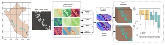
2. Materials and Methods

2.1. Study Area

Peru has the world’s largest concentration of tropical glaciers, covering an estimated area of 1602.96 km² [43]. According to [44], the glacierized areas of the Peruvian Andes can be divided into three subregions based on their temperature, precipitation, and humidity characteristics:

• The sub-region situated in the northern wet outer tropics experiences a high mean annual humidity of 71%, minimal temperature seasonality, and a total annual precipitation of 815 mm. Sub-region 1 includes the Cordillera Blanca, Central, Huallanca, Huayhuash, Huaytapallana, and Raura. Sub-region 2, located in the southern wet outer tropics, has a moderate mean annual humidity of 59%, annual variability of the mean monthly temperature of approximately 4 °C, and a total annual precipitation of 723 mm. Sub-region 2 includes the Cordillera Vilcabamba, Urubamba, and Vilcanota. Sub-region 3 is characterized by a low mean annual humidity of 50%, a mean annual temperature of −4.0 °C, and a minimal total annual precipitation of 287 mm. The three subregions experience a dry season from May to September, coinciding with the austral winter, and a wet season from October to April, corresponding to the austral summer [44]. During the wet season, the glaciers predominantly accumulate mass, while the lower portions of the glaciers experience ablation consistently throughout the year.

This study focuses on sub-regions 1 and 2 (Figure 1). Nevertheless, to ensure the broad applicability of our findings, we carefully select Cordilleras that provide a comprehensive representation of the glacier distribution in Peru, particularly all the selected study areas span proximally 90% of the glaciated surface of the Cordilleras of Perú [9,43]. Blanca (40.20%), Central (3.80%), Huallanca (0.47%), Huayhuash (4.75%), Huaytapallana (1.92%), Raura (2.29%), Urubamba (2.11%), Vilcabamba (9.05%), and Vilcanota (22.96%).

Additionally, the majority of the selected glaciers have been studied in terms of hydrology, ablation, and dynamics, especially the Cordillera Blanca and Cordillera Vilcanota have been intensely studied in recent years [3,11,43,45,46].

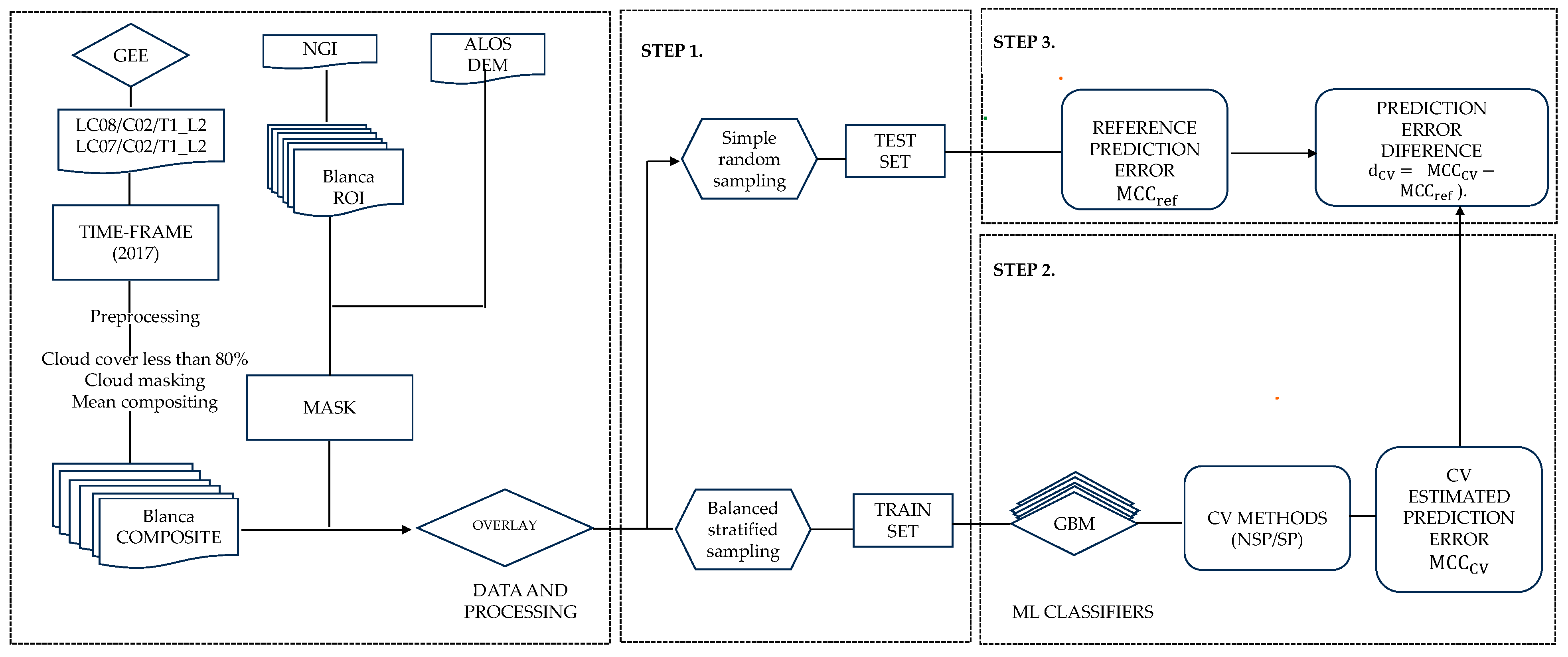
2.2. Data Acquisition

2.2.1. Glacier Inventory

The analysis was conducted using the National Glacier Inventory (NGI) dataset provided by [47] as the reference data. This dataset consisted of polygonal vector data representing glacier areas delineated using mostly Sentinel 2 and Landsat data and high-resolution Google Earth images with field survey studies.

The NGI is a shape file of the 2017–2018 glacier outlines for the main glaciated mountain regions in the Peruvian Andes, covering the entirety of Peru with information concerning their code name, date of acquisition, and remote sensing sensor used for delineation. To prepare the data for classification, the glacier outlines from the NGI were used to generate a binary raster mask with values 0/1 corresponding to non-glacier/glacier pixels.

2.2.2. Landsat Data and Processing

The Landsat data for the period 2017–2018 were acquired from Landsat Collection 2 Level 2 and Tier 1 surface reflectance (SR) products [48] at: https://www.usgs.gov/landsat-missions/landsat-collection-2-surface-reflectance (accessed on 1 July 2023). The Landsat collections were acquired and handled using the Google Earth Engine (GEE) platform [49]. For each selected glacier sub-region, a monthly composite was created using atmospherically corrected and topographic calibrated Landsat 8 OLI reflectance data imagery from the Tier 1 LANDSAT/LC08/C02/T1_L2 collection [49].

All the available images from 2017 with a cloud cover of less than 80% during the dry season (May and September) were filtered. This period corresponds to the end of the ablation period, minimizing the potential confusion caused by transient snow cover, which could degrade the quality of the data and hinder accurate glacier discrimination [11,50]. For the cloud masking, we used the Band Quality Assessment (QA_PIXEL) information available in the Landsat Collection 2 Level 2 and Tier 1 surface reflectance (SR) images. Then we applied a spectral transformation by scale and offset parameters based on [51]. Overall, all the Landsat mosaic composite images cover a total area of 42,135 km² (

Table 1. Properties of each glaciated region.

Cordillera	LS8-7 1 Composite Total Area (km2)	Path/Row	Available Scenes 2
Cordillera Blanca	13,963.1	8, 66 8, 67	30
Cordillera Central	5957.4	7, 68	53
Cordillera Huallanca	271.9	8, 67	21
Cordillera Huayhuash	344.5	8, 67	34
Cordillera Huaytapallana	2489.8	6, 68	9
Cordillera Raura	322.3	7, 67	34
Cordillera Urubamba	1818	4, 69	9
Cordillera Vilcabamba	4221.3	5, 69 4, 69	40
Cordillera Vilcanota	6179.7	3, 69 3, 70	52
Total	42,135

Notes: ¹ Landsat 8 and Landsat 7. ² Scenes that meet filtering criteria.

).

2.2.3. Digital Elevation Model (DEM)

The significance of the topographic characteristics in glacier classification has been demonstrated, as the distinction between debris-covered and non-covered glaciers based solely on reflectance properties is practically impossible [12,29,52]. Accordingly, 10 topographic parameters including elevation, slope, aspect, profile curvature, plan curvature, longitudinal curvature, cross-sectional curvature, maximum curvature, and minimum curvature were generated using SAGA GIS [53] using the 30-m resolution JAXA’S ALOS WORLD 3D DEM downloaded from https://opentopography.org/ (accessed on 2 November 2023) through the R package elevator each glacier region under study.

2.3. Data Overlay

Finally, the spectral and DEM covariates and labels were harmonized to UTM Zone 18S and UTM Zone 19S within sub-regions 1 and 2, respectively. This was done before cropping, resampling to 30 meters, and stacking. With this harmonized dataset, each glacier area was processed one by one in the main workflow, allowing the implementation of modeling methods for individual study areas.

2.4. Machine Learning Classifiers

Like previous cross-validation comparison studies [35,37,40], we selected just a small amount of ML methods for our experiments: random forest, gradient-boosted machines, weighted k-nearest neighbors, and logistic regression. A detailed explanation of each model is outside of the scope of this study, but a summary is given for each model with relevant references for each.

2.4.1. Logistic Regression

Logistic regression (LR) involves a dependent variable represented in binary data, indicating presence (1) and absence (0), and establishes a linear relationship with the independent variable(s) [54]. Through an exponential function (sigmoid function), it computes the classification probability for each input sample. The formulation for multinomial binary logistic regression is as follows:

$$Z=\mathrm{a}+{\sum }_{i=1}^n{b}_i{x}_i$$

(1)

$$P(Z)=\frac{1}{1+e^{-Z}},$$

(2)

where P(Z) is the probability, Z is a parameter, $\mathrm{a}$ is the intercept, $b_i$’s are the coefficients for independent variables $x_i$’s, and the i index is for each covariate. Usually, a probability value of 0.5 serves as a classification threshold, aiding in the computation of classification metrics, such as accuracy.

2.4.2. K-Nearest Neighbors

The weighted k-nearest neighbors (KNN) algorithm is supervised learning that classifies data points by relying on the nearest k samples in the feature space. Using the k-means algorithm provides significant advantages, such as easy interpretation, high flexibility, and computational efficiency [36]. In this research, we implemented KNN using the knnn package for R (https://github.com/KlausVigo/kknn) (accessed on 2 November 2023).

2.4.3. Random Forest

Random forest (RF) belongs to the group of ensemble learners, which builds upon a large number of basic model structures called decision trees (DT) that are trained in parallel. The RF integrates the outcomes of these decision trees (DT) to attain a more accurate and stable prediction compared to a single DT [55]. Currently, the RF is the most common machine learning method used for geospatial predictions [39,56,57,58,59,60,61,62,63].

To train an RF model, some hyper-parameters should be selected, among others, the number of individual decision trees (ntree) and the number of features selected at each split of the trees (mtry). In this study, ntree is kept at a moderate size of 100 to 500. This balance ensures both efficiency and stability [64].

2.4.4. Gradient-Boosting Machines

Gradient-boosting machines (GBM) were first presented in [65], which is another type of model based on ensemble learners. To generate the final prediction results, the GBM could use weak learners in a sequential learning process, in the form of an ensemble of weak predictions such as the DT. Unlike the RF, in the GBM, decision tree learners (DT) are trained sequentially.

All the models were trained using either default hyperparameter values and/or recommendations from the literature that were specifically tailored to our case data. A detailed summary of the models and hyperparameters is shown in

Table 2. Selected hyperparameter data types and chosen values for each algorithm. Notations of hyperparameters from the respective R packages were used.

Algorithm	Reference	Hyperparameter	Type	Default
Gradient-Boosting Machines (GBM) 1	[65]	n.trees	Integer	100
		n.minobsinnode	Integer	10
		shrinkage	Numeric	0.1
		distribution	Nominal	bernoulli
Random Forest (RF)	[55]	num.trees	Integer	500
		mtry	Integer	Sqrt(p)
		min.node.size	Integer	1
		max.depth	Integer	0
Weighted K-Nearest Neighbors (KKN)	https://github.com/KlausVigo/kknn (accessed on 2 November 2023)	k	Integer	10
		distance	Integer	2
		kernel	Nominal	gaussian
Logistic Regression (LR)		family	Nominal	binomial

Notes: ¹ Algorithm symbols used on result’s analysis.

.

2.5. Normalized Difference Snow Index (NDSI)

The normalized difference snow index (NDSI) is widely used to distinguish snow from other land coverages, making it valuable for identifying glacier coverage as well. Subsequently, the NDSI has been extensively used for glacier mapping [6,9,10,11,29]. We computed the NDSI values from each reflectance composite using Equation (3):

$$\mathrm{NDSI}=({\mathsf{\rho }}_{\mathrm{Green}}-{\mathsf{\rho }}_{\mathrm{SWIR}})/({\mathsf{\rho }}_{\mathrm{Green}}+{\mathsf{\rho }}_{\mathrm{SWIR}})$$

(3)

where ${\mathsf{\rho }}_{\mathrm{Green}}$ is the surface reflectance in the green band and ${\mathsf{\rho }}_{\mathrm{SWIR}}$ is the surface reflectance in the SWIR band. The use of the NDSI as the only means of glacier detection is a common approach in glacier mapping generally with acceptable results [50,66,67]. In this work, we utilized the NDSI both as a covariate for machine learning models and as an independent method for delineating glacier outlines for comparison.

2.6. Model Evaluation Metrics

2.6.1. Matthews Correlation Coefficient (MCC)

Assessing binary classifications is a crucial task in statistics and machine learning as it can impact decisions across various domains. To evaluate the accuracy of the models in binary classification problems, we employ the MCC, Equation (4), as an established and robust error measurement metric [68]. The MCC is derived from Cramér’s V and is applied to a 2 × 2 standard confusion matrix, consisting of true positives (TP), true negatives (TN), false negatives (FN), and false positives (FP):

$$\mathrm{CC}=\frac{\mathit{TP}\times \mathit{TN}-\mathit{FP}\times \mathit{FN}}{\sqrt{\left(\mathit{TP}+\mathit{FN}\right)\times \left(\mathit{TP}+\mathit{FN}\right)\times \left(\mathit{TN}+\mathit{FP}\right)\times \left(\mathit{TN}+\mathit{FN}\right)}}$$

(4)

Given the number of experiments we ran in each glacier region, we focused solely on the MCC for sequent comparative analysis because this was proved to be a balanced, more reliable summary of binary classification error than accuracy, F1 score, and Kappa [68,69]. We choose not to use the Kappa coefficient as it has proven not to be a reliable measure of accurate classification and is difficult to interpret [70].

2.6.2. Moran’s I

It is traditionally acknowledged that when applying the standard ML models in a spatial prediction setting, errors could remain dependent in space due to not considering spatial dependency or heterogeneity in crucial explanatory variables [61,71,72]. Preferably the spatial autocorrelation of errors should be minimized or even eliminated [39,40].

Correspondences between predicted and label class data were indicator coded. If the class of the test sampled pixel matched with that of the prediction class, an indicator code 1 was assigned to that sample pixel. In contrast, a code of 0 was assigned to pixels where the predicted class differed from the test class. These values were identified as classification errors and obtained through the 50 repeated 5-fold either spatial or non-spatial cross-validation and then aggregated through a simple majority vote approach for all repetitions. Following that, we explored the spatial autocorrelation of the indicator-coded data using Moran’s I (MI). In all instances, Moran’s I was assessed through the Monte Carlo simulation and calculated from spatial weights matrices based on k = 5 nearest neighbors using the R library spdep [28].

2.6.3. Indicator Variograms

Although cross-validation is a well-established approach for model assessment of supervised machine learning models [16,17,19,35] a particular issue is that spatial autocorrelation in the data can invalidate model validation approaches [39,40]. Therefore, when machine learning models are directly applied to spatial data we need to consider if spatial autocorrelation is present and to what extent [37].

To better understand the effect of spatial autocorrelation in our validation approaches, we test for spatial autocorrelation on class labels using indicator variogram analysis (Equation (5)). The indicator semivariogram ${\gamma }_I$ can be inferred from [27,30,31,32,73]:

$${\gamma }_I\left(U_k;\mathit{h}\right)=\frac{1}{2n\left(h\right)}\sum _{i=i}^{n\left(\mathit{h}\right)}{\left[i\left(U_k;\mathit{x}\right)-i\left(U_k;\mathit{x}+\mathit{h}\pm ∆\mathit{h}\right)\right]}^2;k=1,\dots ,m-1$$

(5)

where $\left\{U_1,\dots ,U_m\right\}$ possible classes exist (in our case two classes for glacier and non-glacier surface, i.e., m = 2), $n\left(\mathit{h}\right)$ is the number of pairs of indicator data that are a distance $\mathit{h}\pm ∆\mathit{h}$ apart, and finally the indicator random function or indicator transform $i\left(U_k;\mathit{x}\right)$ of N ($\mathit{x}$) is defined using Equation (6):

$$I\left(U_k;\mathit{h}\right)=\left\{\begin{array}{c}1 \mathit{if} \mathrm{N}\left(\mathit{x}\right)\in \left\{U_1,\dots ,U_k\right\}\\ 0 \mathit{if} \mathrm{N}\left(\mathit{x}\right)\in \left\{U_{k+1},\dots ,U_m\right\}\end{array}\right.;k=1,\dots ,m-1.$$

(6)

where $\mathrm{N}\left(\mathit{x}\right)$ denotes the value of the random variable at pixel $\mathit{x}$, since we already have binary class labels.

To model the indicator semivariograms for each glacier dataset, we employed various model specifications including the exponential, spherical, Gaussian, and Matern functions. Variograms were fitted by weighted least squares using $N_j/h_j^2$ as weights, where $N_j$ denotes the number of points pairs in the j-th lag and $h_j^2$ is the corresponding lag distance. The model that yielded the smallest residual sum of squares when compared to the sample variogram was selected as the final model. The variogram models were implemented using the gstat package for R [74,75].

2.7. Model Validation

2.7.1. K-Fold Cross-Validation

While the best method is simply using a completely independent test sample, this is not always feasible [76,77]. K-fold cross-validation is a resampling-based technique for the estimation of a model’s predictive performance [78]. The fundamental concept behind K-CV is to divide an existing dataset into training and test sets using a user-defined number of partitions. Initially, the dataset is split into k partitions or folds. The training set comprises k − 1 partitions, and the test set comprises the remaining partitions. A model is trained on the training set and assessed on the test partition, each partition serving as a test set once. In this work, K-fold cross-validation is depicted as non-spatial cross-validation (NSP-CV).

2.7.2. K-Fold Spatial Cross-Validation

The second strategy, known as spatial K-fold CV (SP-CV), differs from NSP-CV by considering the spatial dependence of the data when partitioning observations into subsets. The objective is to group observations into spatially homogeneous clusters beyond the spatial autocorrelation range, thereby achieving independence between cross-validation folds. In this work, we adopted the spatial cross-validation approach proposed by [38] and utilized by [35] which utilizes k-means clustering to mitigate the influence of spatial autocorrelation. In contrast to non-spatial cross-validation, spatial cross-validation partitions the data into spatially disjoint subsets, reducing the impact of spatial autocorrelation. As an example, [39,40] employed k-means clustering to divide samples into five folds according to the locations of sample data. The validity of this procedure was empirically tested by [35,39,79,80]. They found that the SP-CV better approximates the error obtained when predicting species distribution and above-ground forest biomass (AGB).

2.8. Experimental Benchmark

2.8.1. Step 1: Independent Data Test Prediction Error

To evaluate the accuracy of various CV methods, it is crucial to include an unbiased reference prediction error in the benchmarks. Thus, direct implementation of CV methods on the entire dataset is not viable, the initial stage of the experiments involves the creation of training and test datasets for each Cordillera [80] (Figure 2).

For the test data, we employed simple random sampling to generate 1000 independent sampled pixels for each glacier region being investigated, which served as the prediction locations. In contrast, the training samples were selected using a stratified sampling approach to ensure a balanced distribution of the two classes [76,81]. This was done because it has been proven that class imbalances in machine learning models can produce highly biased results [82]. Using randomly independent prediction locations directly as the test set ensures that the calculated value of the reference prediction error, ${\mathrm{MCC}}_{\mathrm{ref}}$, fully captures all unbiased performances of the models [34,77].

2.8.2. Step 2: Compute the Prediction Error for Each CV Method

In this stage, we employed two cross-validation strategies to assess the predictive power of our models and generate the prediction error (${\mathrm{MCC}}_{\mathrm{CV}}$). The first strategy involved NSP-CV. The second cross-validation strategy was SP-CV, in this method, spatial partitions of the sample are created by k-means (k = 5) clustering based on the spatial coordinates, explained in more detail in [35]. The predicted class labels (glacier and non-glacier) were used to calculate the MCC in each case.

In all experiments, k was fixed at 5. Both 10 and 5 represent the most frequently employed values when implementing CV [37]. Then, each CV loop was repeated 50 times (i.e., 50 repeated five-fold partitioning setting was chosen for performance estimation of ${\mathrm{MCC}}_{\mathrm{CV}}$ for each model). Thus, 250 models were fitted and tested at each glacier region and the average ${\mathrm{MCC}}_{\mathrm{CV}}$ was derived to account for random errors [37]. SP-CV also known as blocked spatial cross-validation was implemented using Brennings’ sperrorest package [38].

2.8.3. Step 3: Compute Differences in CV Prediction Errors

Upon completing steps 1 and 2, we acquire the reference prediction error ${\mathrm{MCC}}_{\mathrm{ref}}$ and the prediction error of every model through our two CV methods (${\mathrm{MCC}}_{\mathrm{CV}}$). By comparing them, we can find out which CV method produces overoptimistic classification errors. To achieve this, we employ the CV method’s prediction error difference (${\mathrm{d}}_{\mathrm{CV}}=\left|{\mathrm{MCC}}_{\mathrm{CV}}-{\mathrm{MCC}}_{\mathrm{ref}}\right|$) as a quantitative metric. A value closer to zero suggests that the CV method produces error metrics resembling the actual independent error [80].

2.9. Satistical Comparison of Model Results

To determine the influence of the two different validation scenarios on model performance, a paired t-test was carried out to see if there were significant differences in the results between models. The analysis was based on a modified paired t-test [83] considering as a factor the model and validation strategy used and as a dependent variable the classification performance measure (i.e., MCC). The null hypothesis establishes that average differences between models’ results (i.e., MCC) are negligible, and then both cross-validation approaches behave equally. To analyze the results, we examined the p-values. Before applying the t-test, a Shapiro–Wilk test was conducted to confirm the normal distribution of the experimental results, as required by the test as in [84].

2.10. Software

All modeling analyses were conducted using the R programming language version 4.1.0, an open-source statistical software [85]. The algorithm implementations from several packages were employed, including the gbm (https://github.com/harrysouthworth/gbm (accessed on 2 November 2023) for the boosted regression trees [65], kknn [86] for the weighted k-nearest neighbors classification, ranger [87] for the random forest [55] modeling.

3. Results and Discussion

3.1. Classification Performance

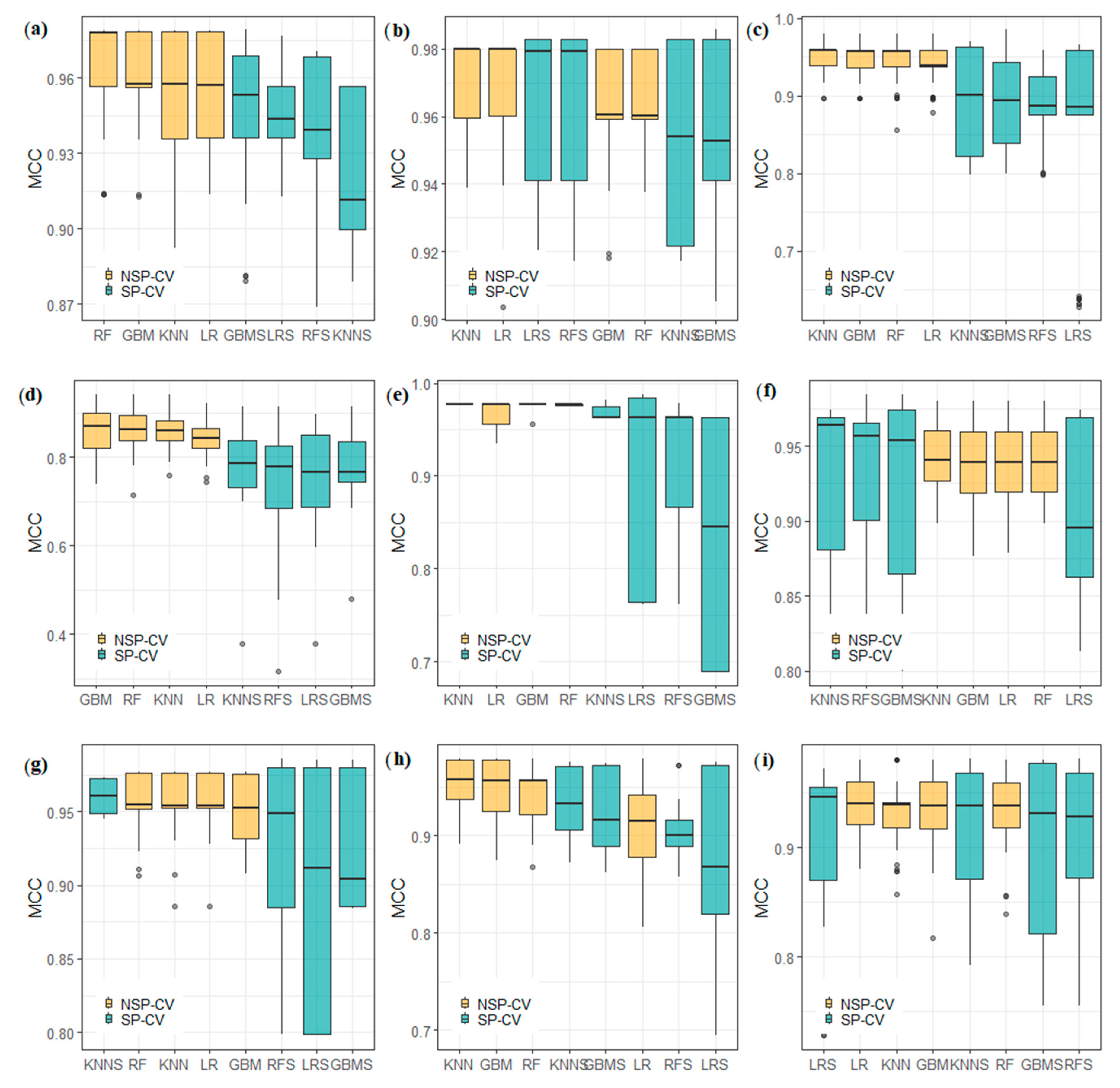
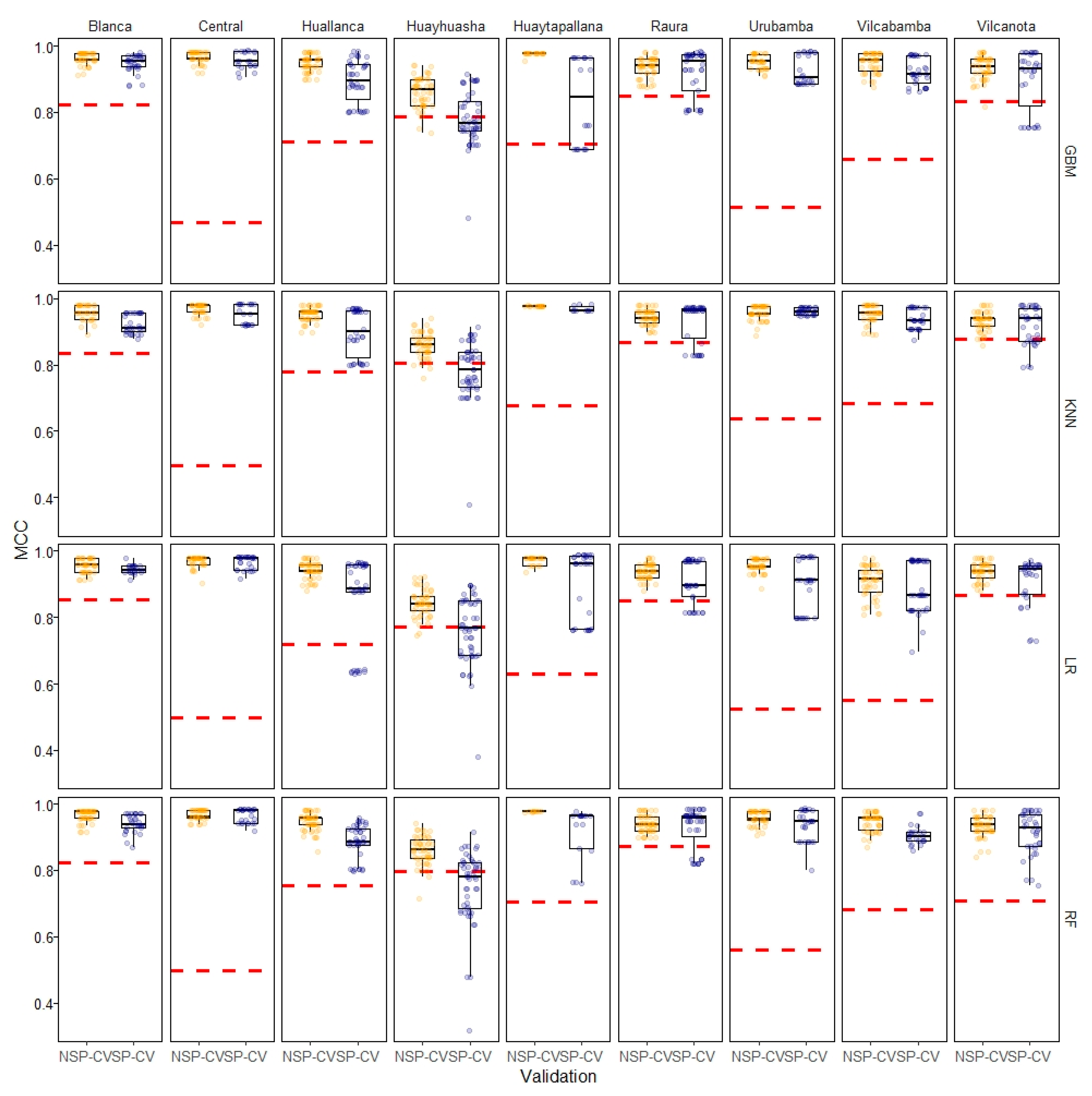
3.1.1. Which Models Showed the Best Performance?

Figure 3 shows the results of our experimental benchmark. It is possible to identify the models that exhibit superior and inferior performance in both scenarios. In the NSP-CV settings, the KNN consistently showed the best performance in all regions, followed by the LR and RF. The SP-CV setting generally shows lower MCC values, the KNN remained as the overall best model in almost all regions, followed by the GBM and LR in the Cordillera Blanca and Central, respectively. Some studies have found that the KNN shows the best predictive performance in spatial settings [86,88] although this is generally not the case [35,89,90,91].

Although the SP-CV generally shows lower MCC results than the NSP-CV, this is not always the case, especially in Cordillera Central, Raura, Urubamba, and Vilcanota. We hypothesize that these results are connected with the degree of spatial autocorrelation/clustering of the glacier class in these specific Cordilleras. For example, the Cordilleras Central and Urubamba present almost a pure nugget effect, which could have generated the mixed response of the MCC to both validation approaches. Hence, it is impossible to distinguish the effect of the SP-CV from the NSP-CV in the presence of weak spatial autocorrelation.

Surprisingly, the LR demonstrates good performance in some cases without clear evidence of being surpassed by models such as the RF and GBM in some cases, as commonly acknowledged in other geospatial contexts [35,56,63]. This outcome emphasizes the significance of traditional parametric approaches in spatial modeling, making this algorithm a reasonable choice, especially when the differences in predictive accuracy compared to the black-box models are minimal.

Concerning the poor performance of the RF, the literature generally agrees upon its general applicability in geospatial contexts as a “go-to” model [35,56,63,66,92]. Since RF uses “bagging”, as spatial data is correlated, this resampling violates the assumption of independence [93] provided evidence that these limitations could lead to inferior prediction performance of the RF under spatial dependence, and this could be the reason for the observed performance of the RF.

3.1.2. Effect of Spatial and Non-spatial Cross-Validation

There were significant differences in the estimated the MCC between the SP-CV and NSP-CV approaches (i.e., ${\mathrm{MCC}}_{\mathrm{SP}-\mathrm{CV}}$ and ${\mathrm{MCC}}_{\mathrm{NSP}-\mathrm{CV}}$). Figure 4 shows the results for both CV methods for each glacier region under study along the reference error $\mathit{refine}$ in red dotted horizontal lines.

First and foremost, it can be seen that almost in all cases the SP-CV and NSP-CV methods produced quite different results in terms of MCC, it’s worth noting that the proposed SP-CV, taking into account the clustered nature of the data, consistently yields evaluation results closer to the reference prediction MCC than the NPS-CV in nearly all cases. This suggests that the SP-CV may produce bias-reduced spatial predictions when using ML models for glacier mapping, especially when training locations are scarce and highly clustered as is usual in glacier monitoring and mapping. As expected, the SP-CV results showed high variances for all models.

Upon careful examination of Figure 4, Cordillera Central, Urubamba, and Vilcabamba, can be found quite high differences between the CV-MCCs and the test MCC (dotted red lines in Figure 4), regardless of the validation approach. It seems that, in those particular cases, both the CV methods are incapable of estimating the true error of the models. This indicates the presence of biased results, even when employing the spatial cross-validation approach suggested in this study. Although there could be multiple reasons to explain these results, we hypothesize that they are due to possible overfitting of the models in those specific areas.

A more detailed analysis can be found in

Table 3. Mean Matthew Correlation Coefficients grouped by Cordillera and CV method.

Glacier Region	SP-CV 1 MCC	NSP-CV 2 MCC
Cordillera Blanca	0.928 (0.0845) 3	0.949 (0.1054)
Cordillera Central	0.937 (0.446)	0.954 (0.4624)
Cordillera Huallanca	0.877 (0.1201)	0.937 (0.1800)
Cordillera Huayhuash	0.753 (0.0196)	0.830 (0.0576)
Cordillera Huaytapallana	0.904 (0.1979)	0.968 (0.2617)
Cordillera Raura	0.915 (0.0532)	0.931 (0.0699)
Cordillera Urubamba	0.906 (0.3082)	0.930 (0.3317)
Cordillera Vilcabamba	0.891 (0.2067)	0.917 (0.2326)
Cordillera Vilcanota	0.906 (0.0618)	0.929 (0.0847)

Notes: ¹ SP-CV: spatial cross-validation, ²: NSP-CV: non-spatial cross-validation, ³: difference regard to the test reference MCC (${\mathrm{MCC}}_{\mathrm{C}}-{\mathrm{MCC}}_{\mathrm{ref}}$) in parenthesis.

which shows the mean MCC grouped by Cordillera and CV method as well the difference regarding the test reference MCC (in parenthesis). For example, Cordillera Blanca’s mean MCC for NSP-CV models is 0.949, while the mean MCC for the SP-CV models is 0.928, and their difference concerning the reference independent test (i.e., ${\mathrm{MCC}}_{\mathrm{ref}}$ 0.844) are 0.1054 and 0.0845, respectively.

Overall, the SP-CV led to a slight decline in the model’s MCC (i.e., about—4%) concerning the NSP-CV method. Likewise, the SP-CV yields a sharp decline in biases ($d_{\mathit{CV}}$). compared to the reference MCC evaluated at the test sets (i.e., about—18%). Moreover, the evaluation results of the SP-CV were significantly closer to the reference prediction error than the results of the NSP-CV for all glacier regions under study. This illustrates that the proposed method, taking into account the spatial structure of the data in the evaluation of the model could indeed provide a reasonable unbiased result. To further strengthen this observation, it is important to analyze the individual model’s discrepancy between the SP-CV and NSP-CV MCC estimates obtained in the benchmark’s settings, which will be explored in the subsequent section.

3.1.3. Statistical Comparison of Model Results

We conducted a comparative statistical analysis of the results.

Table 4. Modified paired t-test, t-statistics, and the p-values (in parenthesis) of paired t-test comparison for the MCC obtained after the 50-repeated 5-fold CV using two types of cross-validation for each glacier region.

Glacier Region	LR	RF	GBM	KNN
Cordillera Blanca	0.05971 (0.4763)	1.155 (0.1267)	1.678 (0.04711) 1	2.061 (0.02229) 1
Cordillera Central	0.2374 (0.4066)	0.8284 (0.2057)	0.6774 (0.2506)	1.391 (0.08516)
Cordillera Huallanca	1.202 (0.1174)	1.9135 (0.03076) 1	1.4590 (0.07545)	1.366 (0.08895)
Cordillera Huayhuash	1.44537 (0.07735)	1.6833 (0.04933) 1	1.64397 (0.05329)	1.64590 (0.0530)
Cordillera Huaytapallana	1.3271 (0.09530)	1.5579 (0.06284)	1.910303 (0.03092) 1	253.484 (-)
Cordillera Raura	0.76974 (0.2225)	0.34939 (0.3641)	0.4885 (0.3136)	0.3651 (0.3582)
Cordillera Urubamba	1.59805 (0.04823) 1	0.93018 (0.1784)	1.2942 (0.1008)	0.0655 (0.4739)
Cordillera Vilcabamba	0.20655 (0.4186)	1.61089 (0.04681) 1	0.9120 (0.1831)	1.3423 (0.09283)
Cordillera Vilcanota	0.84632 (0.2007)	0.62994 (0.2658)	0.7284 (0.2348)	0.48702 (0.3142)

Notes: ¹ Modified paired t-test significance statistical difference between cross-validated MCC results (p-value < 0.05).

shows the t-statistics and the p-values (in parenthesis) of paired t-test comparison for the MCC results obtained after the 50-repeated 5-fold CV using the two types of cross-validation for each glacier region (p-values < 0.05 means that there is a significance statistical difference between cross-validated MCC results and p-value > 0.05 means that both cross-validation approaches yield equal results).

Based on the statistical analysis, considering the results of the paired t-test, it is not definitively conclusive to assert that SP-CV yields significantly different MCC estimates compared to NPS-CV in most cases with the exception of remarkable cases that need further clarification:

For the Cordillera Blanca, only the GBM and KNN models showed significant differences (p-value < 0.05). For Cordillera Huallanca, Huayhuash, and Vilcabamba the RF was the only model that showed significant differences. For Cordillera Huaytapallana, only the GBM showed significant differences. For Cordillera Urubamba, only the LR showed significant differences.

Some algorithms showed no sensitivity to the cross-validation method (i.e., KNN and LR). Since the KNN is the best model overall in all cases regardless of the CV method, this suggests that the KNN can produce more reliable estimates of error and at the same time the best-performing predictions. On the other hand, some algorithms were quite sensible to the cross-validation method. The RF showed significant differences between the SP-CV MCC’s and NP-CV MCC’s. In all those cases, the null hypothesis establishes that average differences between error models (i.e., MCC) are non-negligible. Therefore, this difference can be linked to an overly optimistic bias in nonspatial cross-validation estimates due to spatial autocorrelation [35,37,61,63,80].

However, it should be noted that these results may slightly vary depending on the data distribution within each fold and the randomization in each repetition, which can impact the comparison tests [35]. Nonetheless, given the considerable number of repetitions in the experiments, these results are generally robust.

While our results align with previous studies, such as those by [35,40,94] suggesting that non-spatial performance estimates tend to be significantly “superior” to spatial performance estimates, it is important to note that our experiments do not allow for such a definitive statement in all cases. The observed differences in performance between the spatial and non-spatial estimates in our study may not be as pronounced or statistically significant regardless of the classification algorithm.

3.2. Spatial Autocorrelation Assessment

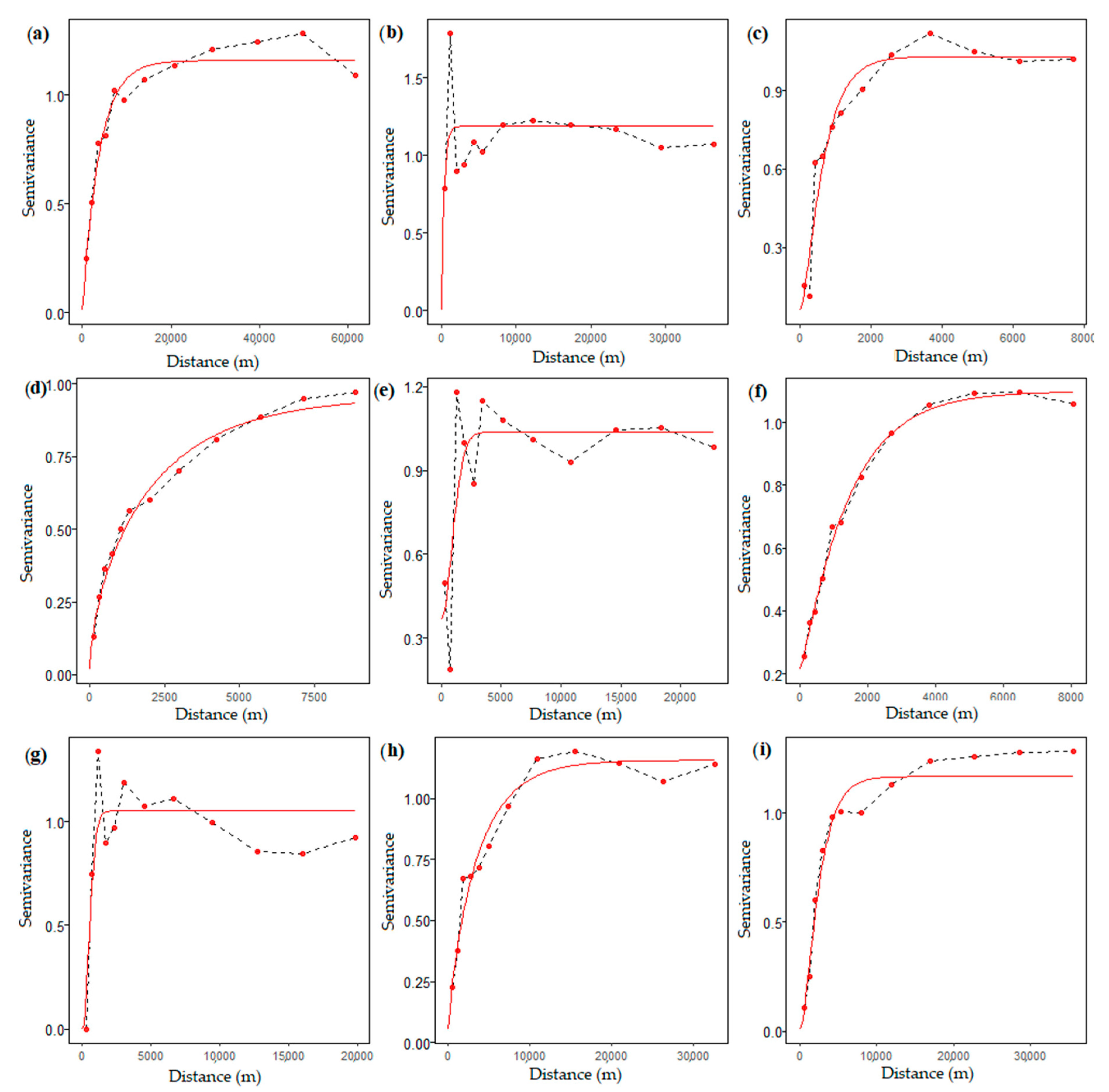
3.2.1. Spatial Autocorrelation of Classes

Semivariograms were calculated for the glacier class indicator variable for each glacier region to confirm the presence of spatial autocorrelation in the datasets.

Figure 5 shows the experimental and fitted indicator variograms for each glacier data set, the variograms were rescaled to enable comparison across datasets. The parameters of the variogram models are given in

Table 5. Rescaled Indicator Variogram Parameters Across glacier regions.

Cordillera	Model 1	Range (m)	C0 2	C 3	Mat-κ 4
Cordillera Blanca	Mat	5428.204	3.57 × 10−4	0.0355	0.5
Cordillera Central	Exp	371.4613	0	0.00475	-
Cordillera Huallanca	Mat	874.5616	1.14 × 10−3	0.0184	1
Cordillera Huayhuash	Mat	3160.411	2.54 × 10−3	0.1477	0.3
Cordillera Huaytapallana	Mat	1320.108	2.21 × 10−3	0.004013	10
Cordillera Raura	Mat	1999.836	1.68 × 10−2	0.07002	0.6
Cordillera Urubamba	Mat	684.1284	0	0.00736	10
Cordillera Vilcabamba	Mat	5326.374	1.30 × 10−3	0.0264	0.4
Cordillera Vilcanota	Mat	3288.231	3.19 × 10−4	0.03816	1.2

Notes: ¹: Mat: Matern, M. Stein’s parameterization; Exp: exponential model. ²: C₀: Nugget effect, and ³ Sill. ⁴: κ (kappa) is a range parameter of the Matern parametrization.

.

In general, the glacier class presents a significant spatial correlation, the smallest range of spatial dependence was found for Cordilleras Central, Urubamba, and Huallanca with ranges from 0.37, 0.68, and 0.87 km, respectively, and the largest range was found for Cordillera Blanca (5.42 km).

For some glacier regions, the variograms exhibit a substantial nugget effect and a structure with a short range. (i.e., Central, Huaytapallana, and Urubamba), as well as bigger kappa parameters, indicating a fairly constant spatial process in those cases. But in general, relatively larger ranges and smaller nugget effects occur for the majority of other regions. For instance, in the Cordillera Blanca case, the indicator variogram shows that at a 30 m resolution km spatial resolution, the glacier class presents a significant spatial correlation up to 5.42 km (Figure 5). This spatial autocorrelation is notably observable in nearly all cases, where clusters of homogeneous glacier class values are present. The Cordillera Blanca region exhibited a larger range due to its considerably larger area (13,963 km²). The absence of similar range behavior in other areas can be attributed to the substantial differences in the overall size and extent of each region because glaciers assume a size and flow rate that are in balance with the local climate [15].

Given the relatively high sampling intensity (and resulting proximity) of glacier class pixels selected for this work, and the long range of spatial autocorrelation in the data, it’s evident that any randomly selected test pixel will not be independent from its neighboring pixels, this circumstance violates the fundamental hypothesis of model validation, specifically, the assumption of independence between training and test sets. This result probably doesn’t hold for the regions for which variograms revealed poor spatial structure like Central, Huaytapallana, and Urubamba Cordilleras. This suggests that a spatial cross-validation method could be useful in this context [37].

It is worth noting that no stationarity assumptions are needed since the indicator variograms are simply used as a means to describe the spatial structure of the data, rather than to perform a model-based inferential spatial prediction of a spatial process.

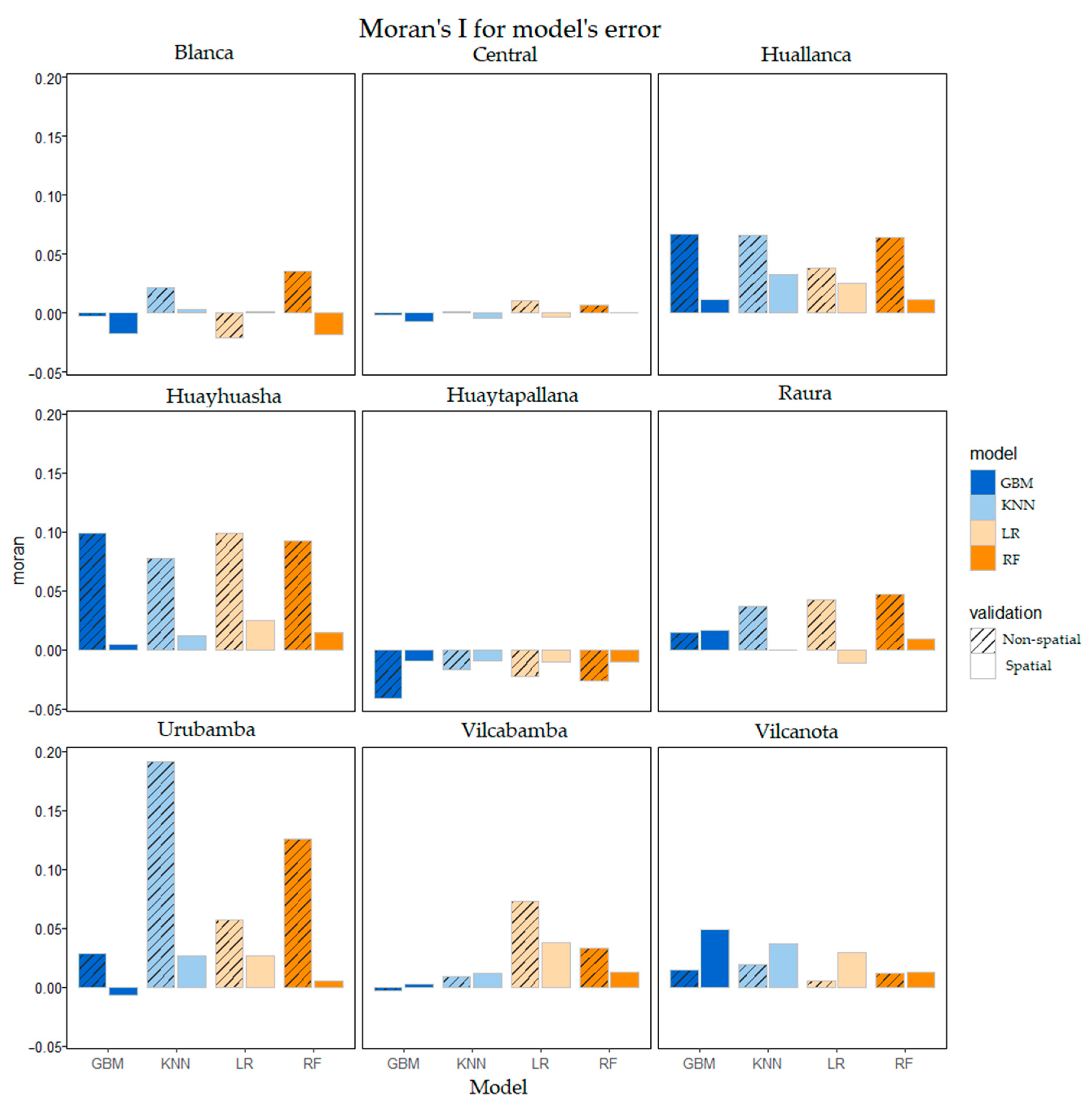
3.2.2. Spatial Autocorrelation of Errors

Figure 6 shows that regardless of the type of modeling algorithm, there were low MI values with statistically non-significant p-values, (i.e., p-values greater than 0.05). At first, it seems that the SP-CV could reduce the spatial dependence of errors compared to the NSP-CV which shows generally higher MI values (i.e., spatially correlated errors). This, suggests that in our SP-CV validation method, the spatial structure of errors is eliminated in all glacier regions but not in the NSP-CV. However, a closer inspection of p-values (not shown in the figure) suggests that the Null hypothesis should not be rejected, and the spatial error patterns are almost random in both cross-validation scenarios.

Urubamba was the only exception in terms of significant MI p-values, especially when the KNN model was applied, indicating the occurrence of spatially correlated errors. Overall, after either the SP-CV or NSP-CV methods, the errors’ spatial structure was completely absorbed by almost all the models in all the glacier regions (statistically non-significant p-values) regardless of the CV approach.

These results suggest that our expectation, wherein the incorporation of spatial information in the SP-CV method is expected to better capture the spatial autocorrelation of errors than the NSP-CV does not hold for glacier classification errors in the Tropical Andes using machine learning algorithms.

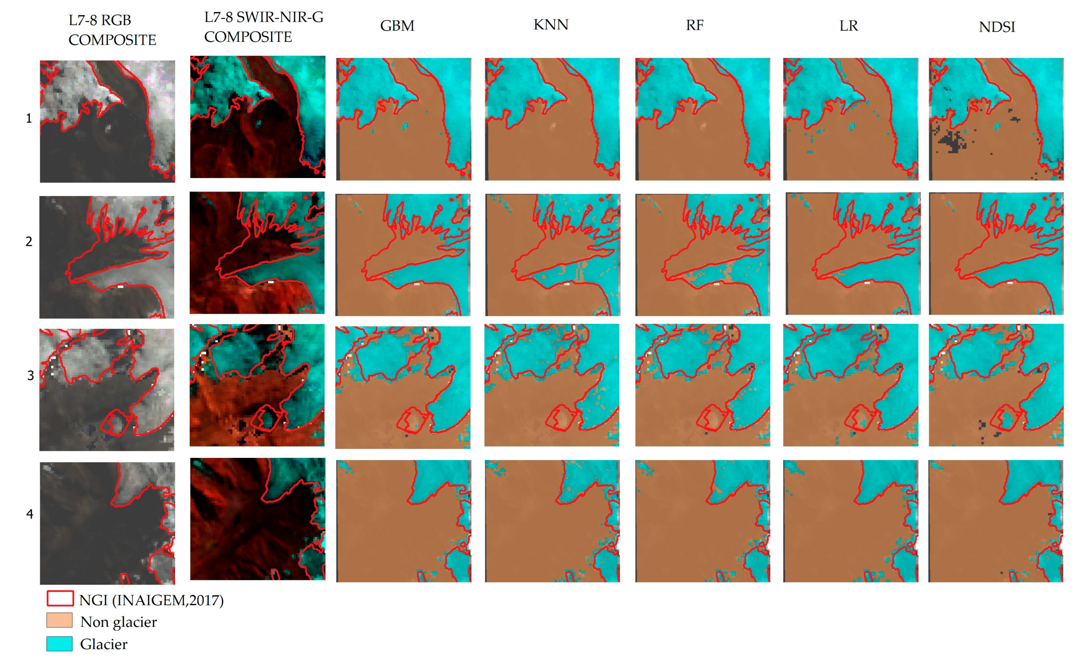
3.3. Spatial Predictions

Finally, we generated glacier outline maps over all studied regions to visually inspect and compare the predictions. For predicting glacier class we took the approach of [95] described in [40]. We used all available pixels of each area to fit the final prediction models. This approach prioritizes the overall quality of the final predictions rather than achieving perfect accuracy in error estimates. The advantage lies in utilizing all available data potentially making it the best predictor, especially for smaller datasets. It has the drawback that the cross-validated errors no longer apply to the predictions, as they were made with different datasets. In this case, as the error estimates will be over-optimistic, the estimated error derived from the SP-CV should be used as the reference error.

To analyze the predictions in greater detail we show a set of predictions on four small areas within the Cordillera Blanca (Figure 7). Overall, the spatial distribution of the model predictions is quite similar. Here, the KNN is not clearly the best predictor all around, as all the outlined maps exhibit a strong agreement with the NGI outline. There are, however, certain areas showing overestimation and underestimation of glacier surfaces. Notably, overestimation is noticeable, particularly near the glacier periphery of the NGI in row 3. In row 2 we observe some areas of underestimation, where glacier areas were misclassified as non-glacier, especially in the case of the KNN and RF algorithms.

These classification errors could be attributed, to some extent, to the compositing and cloud filtering of Landsat 8 images in GEE. This filtering process might lead to the improper detection of transient snow areas, which are then mistaken for glaciers. Importantly, this phenomenon is not observed in other prediction areas. This highlights the significance of the cloud filtering algorithm, as snow pixels can seriously undermine the performance of machine learning models of glacier classification. Additionally, the spatial resolution of Landsat imagery used in this study can introduce a substantial number of mixed pixels—pixels that encompass both the glacier and the surrounding terrain. To address the former issue, a series of recommended algorithms has been previously suggested [50].

The debris-free outline map generated using the NDSI exhibits a high degree of similarity with the NGI outlines, although not perfect, probably due to the NDSI being the current operational method for glacier mapping in Perú [11,47]. Although highly similar, differences exist because our approach uses Landsat 8 imagery, whereas the NGI uses Sentinel 2 and Landsat 8 as well.

Prior studies have already concluded that debris-free ice can be accurately mapped using simple methods, such as the band ratio of the Red/NIR bands of Landsat or S2 data [18,19,20,45,96]. While our primary objective was to compare the predictive classification errors of machine learning algorithms using spatially distributed glacier class data, it’s important to note that the NDSI and band ratio approaches remain robust and widely used methods in remote sensing-based glacier monitoring. As this research demonstrates, these methods should not be dismissed. Nevertheless, evaluating the classification errors of glacier mapping using these approaches requires a proper assessment, typically involving a comparison with high-resolution satellite images [52,96], a procedure that is highly manual and inefficient. Therefore, we hope that a statistically sound approach could enhance current national glacier mapping efforts.

4. Conclusions

In this study, we compared the predictive performance of machine learning algorithms in glacier mapping. We tested k-nearest neighbors, random forests, gradient-boosting machines, and logistic regression in different geographic zones in Peru. Spatial and non-spatial cross-validation methods were used to evaluate the model’s classification errors in terms of the Matthews correlation coefficient (MCC). Performance differences of up to 18% were found between bias-reduced (spatial) and overoptimistic (non-spatial) cross-validation results. Regarding only spatial CV, the k-nearest neighbors (KNN) was the overall best model across Huallanca (0.90), Huayhuasha (0.78), Huaytapallana (0.96), Raura (0.93), Urubamba (0.96), Vilcabamba, (0.93) and Vilcanota (0.92) regions, consistently demonstrating the highest performance followed by logistic regression at Blanca (0.95) and Central (0.97) regions. Although the differences in predictive performance are not statistically significant in all studied regions, we would recommend using spatial CV instead of non-spatial CV for estimating the prediction performance of machine models when mapping glacier landcover, as only this ensures the assessment of bias-reduced predictive performance results, this is especially important when the corresponding results form the basis of policy making.

References

1. Veettil, B.K.; Kamp, U. Remote Sensing of Glaciers in the Tropical Andes: A Review. Int. J. Remote Sens. 2017, 38, 7101–7137. [Google Scholar] [CrossRef]
2. Drenkhan, F.; Carey, M.; Huggel, C.; Seidel, J.; Oré, M.T. The Changing Water Cycle: Climatic and Socioeconomic Drivers of Water-related Changes in the Andes of Peru. WIREs Water 2015, 2, 715–733. [Google Scholar] [CrossRef]
3. Salzmann, N.; Huggel, C.; Rohrer, M.; Silverio, W.; Mark, B.G.; Burns, P.; Portocarrero, C. Glacier Changes and Climate Trends Derived from Multiple Sources in the Data Scarce Cordillera Vilcanota Region, Southern Peruvian Andes. Cryosphere 2013, 7, 103–118. [Google Scholar] [CrossRef]
4. Taylor, L.S.; Quincey, D.J.; Smith, M.W.; Potter, E.R.; Castro, J.; Fyffe, C.L. Multi-Decadal Glacier Area and Mass Balance Change in the Southern Peruvian Andes. Front. Earth Sci. 2022, 10, 863933. [Google Scholar] [CrossRef]
5. Silverio, W.; Jaquet, J.-M. Glacial Cover Mapping (1987–1996) of the Cordillera Blanca (Peru) Using Satellite Imagery. Remote Sens. Environ. 2005, 95, 342–350. [Google Scholar] [CrossRef]
6. Durán-Alarcón, C.; Gevaert, C.M.; Mattar, C.; Jiménez-Muñoz, J.C.; Pasapera-Gonzales, J.J.; Sobrino, J.A.; Silvia-Vidal, Y.; Fashé-Raymundo, O.; Chavez-Espiritu, T.W.; Santillan-Portilla, N. Recent Trends on Glacier Area Retreat over the Group of Nevados Caullaraju-Pastoruri (Cordillera Blanca, Peru) Using Landsat Imagery. J. S. Am. Earth Sci. 2015, 59, 19–26. [Google Scholar] [CrossRef]
7. Juen, I.; Kaser, G.; Georges, C. Modelling Observed and Future Runoff from a Glacierized Tropical Catchment (Cordillera Blanca, Perú). Glob. Planet. Chang. 2007, 59, 37–48. [Google Scholar] [CrossRef]
8. Buytaert, W.; Moulds, S.; Acosta, L.; De Bièvre, B.; Olmos, C.; Villacis, M.; Tovar, C.; Verbist, K.M.J. Glacial Melt Content of Water Use in the Tropical Andes. Environ. Res. Lett. 2017, 12, 114014. [Google Scholar] [CrossRef]
9. Turpo Cayo, E.Y.; Borja, M.O.; Espinoza-Villar, R.; Moreno, N.; Camargo, R.; Almeida, C.; Hopfgartner, K.; Yarleque, C.; Souza, C.M. Mapping Three Decades of Changes in the Tropical Andean Glaciers Using Landsat Data Processed in the Earth Engine. Remote Sens. 2022, 14, 1974. [Google Scholar] [CrossRef]
10. Muñoz, R.; Huggel, C.; Drenkhan, F.; Vis, M.; Viviroli, D. Comparing Model Complexity for Glacio-Hydrological Simulation in the Data-Scarce Peruvian Andes. J. Hydrol. Reg. Stud. 2021, 37, 100932. [Google Scholar] [CrossRef]
11. Veettil, B.K. Glacier Mapping in the Cordillera Blanca, Peru, Tropical Andes, Using Sentinel-2 and Landsat Data. Singap. J. Trop. Geogr. 2018, 39, 351–363. [Google Scholar] [CrossRef]
12. Paul, F.; Barrand, N.E.; Baumann, S.; Berthier, E.; Bolch, T.; Casey, K.; Frey, H.; Joshi, S.P.; Konovalov, V.; Bris, R.L.; et al. On the Accuracy of Glacier Outlines Derived from Remote-Sensing Data. Ann. Glaciol. 2013, 54, 171–182. [Google Scholar] [CrossRef]
13. López-Moreno, J.I.; Fontaneda, S.; Bazo, J.; Revuelto, J.; Azorin-Molina, C.; Valero-Garcés, B.; Morán-Tejeda, E.; Vicente-Serrano, S.M.; Zubieta, R.; Alejo-Cochachín, J. Recent Glacier Retreat and Climate Trends in Cordillera Huaytapallana, Peru. Glob. Planet. Chang. 2014, 112, 1–11. [Google Scholar] [CrossRef]
14. INAIGEM. Manual Metodológico de Inventario Nacional de Glaciares; Instituto Nacional de Investigación en Glaciaresy Ecosistemas de Montaña: Huaraz, Peru, 2017. [Google Scholar]
15. Raup, B.; Racoviteanu, A.; Khalsa, S.J.S.; Helm, C.; Armstrong, R.; Arnaud, Y. The GLIMS Geospatial Glacier Database: A New Tool for Studying Glacier Change. Glob. Planet. Chang. 2007, 56, 101–110. [Google Scholar] [CrossRef]
16. Hastie, T.; Tibshirani, R.; Friedman, J. The Elements of Statistical Learning; Springer Series in Statistics; Springer: New York, NY, USA, 2009; ISBN 978-0-387-84857-0. [Google Scholar]
17. Schratz, P.; Becker, M.; Lang, M.; Brenning, A. Mlr3spatiotempcv: Spatiotemporal Resampling Methods for Machine Learning in R. arXiv 2021, arXiv:2110.12674. [Google Scholar]
18. Alifu, H.; Vuillaume, J.-F.; Johnson, B.A.; Hirabayashi, Y. Machine-Learning Classification of Debris-Covered Glaciers Using a Combination of Sentinel-1/-2 (SAR/Optical), Landsat 8 (Thermal) and Digital Elevation Data. Geomorphology 2020, 369, 107365. [Google Scholar] [CrossRef]
19. Lu, Y.; Zhang, Z.; Shangguan, D.; Yang, J. Novel Machine Learning Method Integrating Ensemble Learning and Deep Learning for Mapping Debris-Covered Glaciers. Remote Sens. 2021, 13, 2595. [Google Scholar] [CrossRef]
20. Baraka, S.; Akera, B.; Aryal, B.; Sherpa, T.; Shresta, F.; Ortiz, A.; Sankaran, K.; Ferres, J.L.; Matin, M.; Bengio, Y. Machine Learning for Glacier Monitoring in the Hindu Kush Himalaya. arXiv 2020, arXiv:2012.05013. [Google Scholar]
21. Caro, A.; Condom, T.; Rabatel, A. Climatic and Morphometric Explanatory Variables of Glacier Changes in the Andes (8–55°S): New Insights From Machine Learning Approaches. Front. Earth Sci. 2021, 9, 713011. [Google Scholar] [CrossRef]
22. Li, X.; Wang, N.; Wu, Y. Automated Glacier Snow Line Altitude Calculation Method Using Landsat Series Images in the Google Earth Engine Platform. Remote Sens. 2022, 14, 2377. [Google Scholar] [CrossRef]
23. Prieur, C.; Rabatel, A.; Thomas, J.-B.; Farup, I.; Chanussot, J. Machine Learning Approaches to Automatically Detect Glacier Snow Lines on Multi-Spectral Satellite Images. Remote Sens. 2022, 14, 3868. [Google Scholar] [CrossRef]
24. Huang, Z. Extensions to the K-Means Algorithm for Clustering Large Data Sets with Categorical Values. Data Min. Knowl. Discov. 1998, 2, 283–304. [Google Scholar] [CrossRef]
25. Khan, A.A.; Jamil, A.; Hussain, D.; Taj, M.; Jabeen, G.; Malik, M.K. Machine-Learning Algorithms for Mapping Debris-Covered Glaciers: The Hunza Basin Case Study. IEEE Access 2020, 8, 12725–12734. [Google Scholar] [CrossRef]
26. Zhang, J.; Jia, L.; Menenti, M.; Hu, G. Glacier Facies Mapping Using a Machine-Learning Algorithm: The Parlung Zangbo Basin Case Study. Remote Sens. 2019, 11, 452. [Google Scholar] [CrossRef]
27. Bierkens, M.F.P.; Burrough, P.A. The Indicator Approach to Categorical Soil Data. J. Soil Sci. 1993, 44, 361–368. [Google Scholar] [CrossRef]
28. Bivand, R.S.; Pebesma, E.; Gómez-Rubio, V. Applied Spatial Data Analysis with R; Springer: New York, NY, USA, 2013; ISBN 978-1-4614-7617-7. [Google Scholar]
29. Burns, P.; Nolin, A. Using Atmospherically-Corrected Landsat Imagery to Measure Glacier Area Change in the Cordillera Blanca, Peru from 1987 to 2010—ScienceDirect. Remote Sens. Environ. 2014, 140, 165–178. [Google Scholar] [CrossRef]
30. Cressie, N.A.C. Statistics for Spatial Data, Revised Edition; John Wiley & Sons, Inc.: Hoboken, NJ, USA, 2015; ISBN 978-1-119-11517-5. [Google Scholar]
31. Easterling, W.; Apps, M. Assessing the Consequences of Climate Change for Food and Forest Resources: A View from the IPCC. In Increasing Climate Variability and Change; Salinger, J., Sivakumar, M.V.K., Motha, R.P., Eds.; Springer: Berlin/Heidelberg, Germany, 2005; pp. 165–189. ISBN 978-1-4020-3354-4. [Google Scholar]
32. Tsendbazar, N.-E.; De Bruin, S.; Fritz, S.; Herold, M. Spatial Accuracy Assessment and Integration of Global Land Cover Datasets. Remote Sens. 2015, 7, 15804–15821. [Google Scholar] [CrossRef]
33. Brenning, A. Spatial Prediction Models for Landslide Hazards: Review, Comparison and Evaluation. Nat. Hazards Earth Syst. Sci. 2005, 5, 853–862. [Google Scholar] [CrossRef]
34. De Bruin, S.; Brus, D.J.; Heuvelink, G.B.M.; Van Ebbenhorst Tengbergen, T.; Wadoux, A.M.J.-C. Dealing with Clustered Samples for Assessing Map Accuracy by Cross-Validation. Ecol. Inform. 2022, 69, 101665. [Google Scholar] [CrossRef]
35. Schratz, P.; Muenchow, J.; Iturritxa, E.; Richter, J.; Brenning, A. Hyperparameter Tuning and Performance Assessment of Statistical and Machine-Learning Algorithms Using Spatial Data. Ecol. Model. 2019, 406, 109–120. [Google Scholar] [CrossRef]
36. Kopczewska, K. Spatial Machine Learning: New Opportunities for Regional Science. Ann. Reg. Sci. 2022, 68, 713–755. [Google Scholar] [CrossRef]
37. Ploton, P.; Mortier, F.; Réjou-Méchain, M.; Barbier, N.; Picard, N.; Rossi, V.; Dormann, C.; Cornu, G.; Viennois, G.; Bayol, N.; et al. Spatial Validation Reveals Poor Predictive Performance of Large-Scale Ecological Mapping Models. Nat. Commun. 2020, 11, 4540. [Google Scholar] [CrossRef] [PubMed]
38. Brenning, A. Spatial Cross-Validation and Bootstrap for the Assessment of Prediction Rules in Remote Sensing: The R Package Sperrorest. In Proceedings of the 2012 IEEE International Geoscience and Remote Sensing Symposium, Munich, Germany, 22–27 July 2012; pp. 5372–5375. [Google Scholar]
39. Milà, C.; Mateu, J.; Pebesma, E.; Meyer, H. Nearest Neighbour Distance Matching Leave-One-Out Cross-Validation for Map Validation. Methods Ecol. Evol. 2022, 13, 1304–1316. [Google Scholar] [CrossRef]
40. Roberts, D.R.; Bahn, V.; Ciuti, S.; Boyce, M.S.; Elith, J.; Guillera-Arroita, G.; Hauenstein, S.; Lahoz-Monfort, J.J.; Schröder, B.; Thuiller, W.; et al. Cross-Validation Strategies for Data with Temporal, Spatial, Hierarchical, or Phylogenetic Structure. Ecography 2017, 40, 913–929. [Google Scholar] [CrossRef]
41. Rocha, A.; Groen, T.; Skidmore, A.; Darvishzadeh, R.; Willemen, L. Machine Learning Using Hyperspectral Data Inaccurately Predicts Plant Traits Under Spatial Dependency. Remote Sens. 2018, 10, 1263. [Google Scholar] [CrossRef]
42. Meyer, H.; Pebesma, E. Machine Learning-Based Global Maps of Ecological Variables and the Challenge of Assessing Them. Nat. Commun. 2022, 13, 2208. [Google Scholar] [CrossRef] [PubMed]
43. Seehaus, T.; Malz, P.; Sommer, C.; Lippl, S.; Cochachin, A.; Braun, M. Changes of the Tropical Glaciers throughout Peru between 2000 and 2016—Mass Balance and Area Fluctuations. Cryosphere 2019, 13, 2537–2556. [Google Scholar] [CrossRef]
44. Sagredo, E.A.; Lowell, T.V. Climatology of Andean Glaciers: A Framework to Understand Glacier Response to Climate Change. Glob. Planet. Chang. 2012, 86–87, 101–109. [Google Scholar] [CrossRef]
45. Drenkhan, F.; Guardamino, L.; Huggel, C.; Frey, H. Current and Future Glacier and Lake Assessment in the Deglaciating Vilcanota-Urubamba Basin, Peruvian Andes. Glob. Planet. Chang. 2018, 169, 105–118. [Google Scholar] [CrossRef]
46. Kozhikkodan Veettil, B.; de Souza, S.F. Study of 40-Year Glacier Retreat in the Northern Region of the Cordillera Vilcanota, Peru, Using Satellite Images: Preliminary Results. Remote Sens. Lett. 2017, 8, 78–85. [Google Scholar] [CrossRef]
47. INAIGEM. Inventario Nacional de Glaciares; Instituto Nacional de Investigación en Glaciaresy Ecosistemas de Montaña: Huaraz, Peru, 2018. [Google Scholar]
48. Vermote, E.; Justice, C.; Claverie, M.; Franch, B. Preliminary Analysis of the Performance of the Landsat 8/OLI Land Surface Reflectance Product. Remote Sens. Environ. 2016, 185, 46–56. [Google Scholar] [CrossRef] [PubMed]
49. Gorelick, N.; Hancher, M.; Dixon, M.; Ilyushchenko, S.; Thau, D.; Moore, R. Google Earth Engine: Planetary-Scale Geospatial Analysis for Everyone. Remote Sens. Environ. 2017, 202, 18–27. [Google Scholar] [CrossRef]
50. Paul, F.; Bolch, T.; Kääb, A.; Nagler, T.; Nuth, C.; Scharrer, K.; Shepherd, A.; Strozzi, T.; Ticconi, F.; Bhambri, R.; et al. The Glaciers Climate Change Initiative: Methods for Creating Glacier Area, Elevation Change and Velocity Products. Remote Sens. Environ. 2015, 162, 408–426. [Google Scholar] [CrossRef]
51. Roy, D.P.; Kovalskyy, V.; Zhang, H.K.; Vermote, E.F.; Yan, L.; Kumar, S.S.; Egorov, A. Characterization of Landsat-7 to Landsat-8 Reflective Wavelength and Normalized Difference Vegetation Index Continuity. Remote Sens. Environ. 2016, 185, 57–70. [Google Scholar] [CrossRef] [PubMed]
52. Paul, F.; Huggel, C.; Kääb, A. Combining Satellite Multispectral Image Data and a Digital Elevation Model for Mapping Debris-Covered Glaciers. Remote Sens. Environ. 2004, 89, 510–518. [Google Scholar] [CrossRef]
53. Conrad, O.; Bechtel, B.; Bock, M.; Dietrich, H.; Fischer, E.; Gerlitz, L.; Wehberg, J.; Wichmann, V.; Böhner, J. System for Automated Geoscientific Analyses (SAGA) v. 2.1.4. Geosci. Model Dev. 2015, 8, 1991–2007. [Google Scholar] [CrossRef]
54. Das, P.; Pandey, V. Use of Logistic Regression in Land-Cover Classification with Moderate-Resolution Multispectral Data. J. Indian Soc. Remote Sens. 2019, 47, 1443–1454. [Google Scholar] [CrossRef]
55. Breiman, L. Random Forests. Mach. Learn. 2001, 45, 5–32. [Google Scholar] [CrossRef]
56. Hengl, T.; Nussbaum, M.; Wright, M.N.; Heuvelink, G.B.M.; Gräler, B. Random Forest as a Generic Framework for Predictive Modeling of Spatial and Spatio-Temporal Variables. PeerJ 2018, 6, e5518. [Google Scholar] [CrossRef]
57. Meyer, H.; Reudenbach, C.; Wöllauer, S.; Nauss, T. Importance of Spatial Predictor Variable Selection in Machine Learning Applications—Moving from Data Reproduction to Spatial Prediction. Ecol. Model. 2019, 411, 108815. [Google Scholar] [CrossRef]
58. Gupta, S.; Papritz, A.; Lehmann, P.; Hengl, T.; Bonetti, S.; Or, D. Global Mapping of Soil Water Characteristics Parameters—Fusing Curated Data with Machine Learning and Environmental Covariates. Remote Sens. 2022, 14, 1947. [Google Scholar] [CrossRef]
59. Chen, Q.; Miao, F.; Wang, H.; Xu, Z.; Tang, Z.; Yang, L.; Qi, S. Downscaling of Satellite Remote Sensing Soil Moisture Products Over the Tibetan Plateau Based on the Random Forest Algorithm: Preliminary Results. Earth Space Sci. 2020, 7, e2020EA001265. [Google Scholar] [CrossRef]
60. de Graaf, I.E.M.; Sutanudjaja, E.H.; van Beek, L.P.H.; Bierkens, M.F.P. A High-Resolution Global-Scale Groundwater Model. Hydrol. Earth Syst. Sci. 2015, 19, 823–837. [Google Scholar] [CrossRef]
61. Georganos, S.; Grippa, T.; Niang Gadiaga, A.; Linard, C.; Lennert, M.; Vanhuysse, S.; Mboga, N.; Wolff, E.; Kalogirou, S. Geographical Random Forests: A Spatial Extension of the Random Forest Algorithm to Address Spatial Heterogeneity in Remote Sensing and Population Modelling. Geocarto Int. 2021, 36, 121–136. [Google Scholar] [CrossRef]
62. Hu, L.; Chun, Y.; Griffith, D.A. Incorporating Spatial Autocorrelation into House Sale Price Prediction Using Random Forest Model. Trans. GIS 2022, 26, 2123–2144. [Google Scholar] [CrossRef]
63. Sekulić, A.; Kilibarda, M.; Heuvelink, G.B.M.; Nikolić, M.; Bajat, B. Random Forest Spatial Interpolation. Remote Sens. 2020, 12, 1687. [Google Scholar] [CrossRef]
64. Probst, P.; Wright, M.N.; Boulesteix, A. Hyperparameters and Tuning Strategies for Random Forest. WIREs Data Min. Knowl. Discov. 2019, 9, e1301. [Google Scholar] [CrossRef]
65. Friedman, J.H. Stochastic Gradient Boosting. Comput. Stat. Data Anal. 2002, 38, 367–378. [Google Scholar] [CrossRef]
66. Wang, J.; Tang, Z.; Deng, G.; Hu, G.; You, Y.; Zhao, Y. Landsat Satellites Observed Dynamics of Snowline Altitude at the End of the Melting Season, Himalayas, 1991–2022. Remote Sens. 2023, 15, 2534. [Google Scholar] [CrossRef]
67. Wang, X.; Wang, J.; Che, T.; Huang, X.; Hao, X.; Li, H. Snow Cover Mapping for Complex Mountainous Forested Environments Based on a Multi-Index Technique. IEEE J. Sel. Top. Appl. Earth Obs. Remote Sens. 2018, 11, 1433–1441. [Google Scholar] [CrossRef]
68. Chicco, D.; Warrens, M.J.; Jurman, G. The Matthews Correlation Coefficient (MCC) Is More Informative Than Cohen’s Kappa and Brier Score in Binary Classification Assessment. IEEE Access 2021, 9, 78368–78381. [Google Scholar] [CrossRef]
69. Chicco, D.; Jurman, G. The Advantages of the Matthews Correlation Coefficient (MCC) over F1 Score and Accuracy in Binary Classification Evaluation. BMC Genom. 2020, 21, 6. [Google Scholar] [CrossRef] [PubMed]
70. Foody, G.M. Explaining the Unsuitability of the Kappa Coefficient in the Assessment and Comparison of the Accuracy of Thematic Maps Obtained by Image Classification. Remote Sens. Environ. 2020, 239, 111630. [Google Scholar] [CrossRef]
71. Jiang, Z. A Survey on Spatial Prediction Methods. IEEE Trans. Knowl. Data Eng. 2019, 31, 1645–1664. [Google Scholar] [CrossRef]
72. Liu, X.; Kounadi, O.; Zurita-Milla, R. Incorporating Spatial Autocorrelation in Machine Learning Models Using Spatial Lag and Eigenvector Spatial Filtering Features. ISPRS Int. J. Geo-Inf. 2022, 11, 242. [Google Scholar] [CrossRef]
73. Goovaerts, P. AUTO-IK: A 2D Indicator Kriging Program for the Automated Non-Parametric Modeling of Local Uncertainty in Earth Sciences. Comput. Geosci. 2009, 35, 1255–1270. [Google Scholar] [CrossRef]
74. Pebesma, E.; Bivand, R.S. Classes and Methods for Spatial Data: The Sp Package. R News 2005, 5, 9–13. [Google Scholar]
75. Gräler, B.; Pebesma, E.; Heuvelink, G. Spatio-Temporal Interpolation Using Gstat. R J. 2016, 8, 204. [Google Scholar] [CrossRef]
76. Brus, D.J.; Kempen, B.; Heuvelink, G.B.M. Sampling for Validation of Digital Soil Maps. Eur. J. Soil Sci. 2011, 62, 394–407. [Google Scholar] [CrossRef]
77. Wadoux, A.M.J.-C.; Heuvelink, G.B.M.; de Bruin, S.; Brus, D.J. Spatial Cross-Validation Is Not the Right Way to Evaluate Map Accuracy. Ecol. Model. 2021, 457, 109692. [Google Scholar] [CrossRef]
78. James, G.; Witten, D.; Hastie, T.; Tibshirani, R. An Introduction to Statistical Learning: With Applications in R.; Springer Texts in Statistics; Springer: New York, NY, USA, 2013; ISBN 978-1-4614-7137-0. [Google Scholar]
79. Gao, B.; Stein, A.; Wang, J. A Two-Point Machine Learning Method for the Spatial Prediction of Soil Pollution. Int. J. Appl. Earth Obs. Geoinf. 2022, 108, 102742. [Google Scholar] [CrossRef]
80. Wang, Y.; Khodadadzadeh, M.; Zurita-Milla, R. Spatial+: A New Cross-Validation Method to Evaluate Geospatial Machine Learning Models. Int. J. Appl. Earth Obs. Geoinf. 2023, 121, 103364. [Google Scholar] [CrossRef]
81. Walvoort, D.J.J.; Brus, D.J.; de Gruijter, J.J. An R Package for Spatial Coverage Sampling and Random Sampling from Compact Geographical Strata by K-Means. Comput. Geosci. 2010, 36, 1261–1267. [Google Scholar] [CrossRef]
82. Chabalala, Y.; Adam, E.; Ali, K.A. Exploring the Effect of Balanced and Imbalanced Multi-Class Distribution Data and Sampling Techniques on Fruit-Tree Crop Classification Using Different Machine Learning Classifiers. Geomatics 2023, 3, 70–92. [Google Scholar] [CrossRef]
83. Nadeau, C.; Bengio, Y. Inference for the Generalization Error. Mach. Learn. 2003, 52, 239–281. [Google Scholar] [CrossRef]
84. Guillén, A.; Martínez, J.; Carceller, J.M.; Herrera, L.J. A Comparative Analysis of Machine Learning Techniques for Muon Count in UHECR Extensive Air-Showers. Entropy 2020, 22, 1216. [Google Scholar] [CrossRef] [PubMed]
85. R Core Team. R: A Language and Environment for Statistical Computing; R Foundation for Statistical Computing: Vienna, Austria, 2013. [Google Scholar]
86. Uddin, S.; Haque, I.; Lu, H.; Moni, M.A.; Gide, E. Comparative Performance Analysis of K-Nearest Neighbour (KNN) Algorithm and Its Different Variants for Disease Prediction. Sci. Rep. 2022, 12, 6256. [Google Scholar] [CrossRef] [PubMed]
87. Wright, M.N.; Ziegler, A. Ranger: A Fast Implementation of Random Forests for High Dimensional Data. J. Stat. Soft. 2017, 77, 1–17. [Google Scholar] [CrossRef]
88. Pacheco, A.D.P.; Junior, J.A.D.S.; Ruiz-Armenteros, A.M.; Henriques, R.F.F. Assessment of K-Nearest Neighbor and Random Forest Classifiers for Mapping Forest Fire Areas in Central Portugal Using Landsat-8, Sentinel-2, and Terra Imagery. Remote Sens. 2021, 13, 1345. [Google Scholar] [CrossRef]
89. Bansal, M.; Goyal, A.; Choudhary, A. A Comparative Analysis of K-Nearest Neighbor, Genetic, Support Vector Machine, Decision Tree, and Long Short Term Memory Algorithms in Machine Learning. Decis. Anal. J. 2022, 3, 100071. [Google Scholar] [CrossRef]
90. Hoef, J.M.V.; Temesgen, H. A Comparison of the Spatial Linear Model to Nearest Neighbor (k-NN) Methods for Forestry Applications. PLoS ONE 2013, 8, e59129. [Google Scholar] [CrossRef]
91. Vega Isuhuaylas, L.A.; Hirata, Y.; Ventura Santos, L.C.; Serrudo Torobeo, N. Natural Forest Mapping in the Andes (Peru): A Comparison of the Performance of Machine-Learning Algorithms. Remote Sens. 2018, 10, 782. [Google Scholar] [CrossRef]
92. Behrens, T.; Viscarra Rossel, R.A. On the Interpretability of Predictors in Spatial Data Science: The Information Horizon. Sci. Rep. 2020, 10, 16737. [Google Scholar] [CrossRef]
93. Saha, A.; Basu, S.; Datta, A. Random Forests for Spatially Dependent Data. J. Am. Stat. Assoc. 2023, 118, 665–683. [Google Scholar] [CrossRef]
94. Meyer, H.; Reudenbach, C.; Hengl, T.; Katurji, M.; Nauss, T. Improving Performance of Spatio-Temporal Machine Learning Models Using Forward Feature Selection and Target-Oriented Validation. Environ. Model. Softw. 2018, 101, 1–9. [Google Scholar] [CrossRef]
95. Kuhn, M. Building Predictive Models in R Using the Caret Package. J. Stat. Soft. 2008, 28, 1–26. [Google Scholar] [CrossRef]
96. Kochtitzky, W.H.; Edwards, B.R.; Enderlin, E.M.; Marino, J.; Marinque, N. Improved Estimates of Glacier Change Rates at Nevado Coropuna Ice Cap, Peru. J. Glaciol. 2018, 64, 175–184. [Google Scholar] [CrossRef]
Figure 1. The geographical location of the selected study areas in this work, Perú. The background is a JAXA’S ALOS WORLD 3D DEM and references glacier surfaces from the National Inventory of Glaciers produced in 2017. All the plotting was done in QGIS 3.30.1-’s-Hertogenbosch.
Water 15 04214 g001
Figure 2. Flowchart of the Processing Steps Presented in This Study.
Water 15 04214 g002
Figure 3. The final results (Matthew correlation coefficient MCC CV ) of experimental benchmarks on the nine studied areas: (a) Blanca, (b) Central, (c) Huallanca, (d) Huayhuasha, (e) Huaytapallana, (f) Raura, (g) Urubamba, (h) Vilcabamba, and (i) Vilcanota. Dots are outliers that stay out of the interval [Q1 − 1.5 × IQR; Q3 + 1.5 × IQR].
Water 15 04214 g003
Figure 4. The final results (Matthew correlation coefficient MCC CV ) of experimental benchmarks were segregated by model type and study area. Reference error of each model MCC ref in red dotted horizontal lines are used for calculated d CV = MCC CV MCC ref .
Water 15 04214 g004
Figure 5. Experimental (points) and fitted rescaled indicator variograms (curves) for the data set with 1000 pixels. (a) Blanca, (b) Central, (c) Huallanca, (d) Huayhuasha, (e) Huaytapallana, (f) Raura, (g) Urubamba, (h) Vilcabamba, and (i) Vilcanota. Dots are experimental varioagrams and red lines are fitted model variograms.
Water 15 04214 g005
Figure 6. Moran’s I result of cross-validation error.
Water 15 04214 g006
Figure 7. Maps of the spatial predictions of compared models. NDSI is added as a comparison. Reference National Glacier Inventory in red contour is overlaid as a reference [14]. Numbers 1–4 represent 4 rectangular zones within Vilcanota region, for sake of visualization.
Water 15 04214 g007