
Landsat Satellites Observed Dynamics of Snowline Altitude at the End of the Melting Season, Himalayas, 1991–2022

1
National-Local Joint Engineering Laboratory of Geo-Spatial Information Technology, Hunan University of Science and Technology, Xiangtan 411201, China
2
School of Geography and Information Engineering, China University of Geosciences (Wuhan), Wuhan 430074, China
3
State Key Laboratory of Cryospheric Science, Northwest Institute of Eco-Environment and Resources, Chinese Academy of Sciences, Lanzhou 730000, China
4
School of Geography and Tourism, Anhui Normal University, Wuhu 241002, China
*
Author to whom correspondence should be addressed.
Remote Sens. 2023, 15(10), 2534; https://doi.org/10.3390/rs15102534
Submission received: 7 April 2023
/
Revised: 8 May 2023
/
Accepted: 9 May 2023
/
Published: 11 May 2023
(This article belongs to the Special Issue Monitoring Cold-Region Water Cycles Using Remote Sensing Big Data)
Abstract
:Studying the dynamics of snowline altitude at the end of the melting season (SLA-EMS) is beneficial in predicting future trends of glaciers and non-seasonal snow cover and in comprehending regional and global climate change. This study investigates the spatiotemporal variation characteristics of SLA-EMS in nine glacier areas of the Himalayas, utilizing Landsat images from 1991 to 2022. The potential correlations between SLA-EMS, alterations in temperature, and variations in precipitation across the Himalayas region glacier are also being analyzed. The results obtained are summarized below: (1) the Landsat-extracted SLA-EMS exhibits a strong agreement with the minimum snow coverage at the end of the melting season derived from Sentinel-2, achieving an overall accuracy (OA) of 92.6% and a kappa coefficient of 0.85. The SLA-EMS can be accurately obtained by using this model. (2) In the last 30 years, the SLA-EMS in the study areas showed an upward trend, with the rising rate ranging from 0.4 m·a−1 to 9.4 m·a−1. Among them, the SLA-EMS of Longbasaba rose fastest, and that of Namunani rose slowest. (3) The SLA-EMS in different regions of the Himalayas in a W-E direction have different sensitivity to precipitation and temperature. However, almost all of them show a positive correlation with temperature and a negative correlation with precipitation.
1. Introduction
Snow cover plays an important role in many ecological, climatic, and hydrological processes in mountain regions and high latitudes. Investigating the variations in snow cover holds immense significance in scrutinizing and preserving water management practices for eco-systemic processes and irrigation purposes, since more than one sixth of the world’s population depends on water sourced from mountainous snow melt [1,2,3]. The snowline serves as the boundary separating snow covered area from snow-free areas on the earth’s land surface [4], the snowline altitude (SLA), and its inter- and intra-annual fluctuations constitute crucial traits that reflect the temporal transformations in snow cover and the duration of snow melting [5]. In the middle latitudes, seasonal changes can cause the position of the snowline to rise or fall [6,7], this temporary boundary is also called the seasonal snowline (or the transient snowline) [8,9,10,11]. In the field of glaciology, the snowline refers specifically to the lower limit of snow cover at the end of the melting season, equivalent to the snowline altitude at the end of the melting season (SLA-EMS) [12,13,14]. The SLA-EMS serves as a reliable symbol of the equilibrium line altitude (ELA) on glaciers and is frequently utilized to signify the mass balance of glaciers [12,13,14,15,16,17]. The fall or rise of SLA-EMS directly reflects glaciers’ advance and retreat. As an important climate change indicator, the study of SLA-EMS helps predict the future trend of glaciers and non-seasonal snow cover and to understand regional and global climate change [18,19,20]. This research holds immense significance for managing water resources in the cryosphere and ensuring their sustainability.
The Himalayas host approximately 15,000 glaciers, many of which are proglacial and rapidly retreating [21]. The Himalayan region consists of a chain of mountains, valleys, and basins, with copious snow cover, representing an extremely vulnerable area that responds acutely to regional and global climate alterations. In general, the glaciers situated in the Himalayas have been in a state of recession since the year 1850 [22]. The loss of snow and ice in the Himalayas during the last century has exceeded the rates of change recorded anywhere else in the world over a comparable timeframe [23,24]. Perennial snow and ice melt from the three primary Himalayan River systems (i.e., the Brahmaputra, Indus, and Ganga) are utilized for various purposes such as irrigation, hydroelectric power generation, bio-resource production, and meeting local water demands in catchments and alluvial plains [25]. Monitoring changes in SLA in the Himalayas using remote sensing, and exploring their correlation with climate variables, can offer valuable insights into the effects of climate change on regional hydrology.
The employment of remote sensing technology has emerged as a significant approach for conducting cryosphere research [26,27,28,29,30]. Using satellite remote sensing, it is possible to extract and assess the snowline in regions that are challenging to reach due to their rugged topography and severe weather conditions [31,32]. MODIS snow cover products are extensively utilized for monitoring seasonal (or transient) snowline altitude over a large area due to their high temporal resolution [5,16,33,34,35,36]. However, the spatial resolution of MODIS snow cover products is limited, which makes it unsuitable for monitoring SLA-EMS in small areas [13]. In contrast, Landsat images provide long-term and high-resolution remote sensing data but have not been fully utilized due to challenges related to storage and processing [6,17,37,38]. The Google Earth Engine (GEE) is a cloud computing platform that facilitates access to powerful computing resources for analyzing large geospatial datasets [39,40]. The potential of GEE for snow mapping and monitoring of snowlines has been demonstrated in several studies [32,41,42]. Further research is necessary to develop an effective approach for estimating continuous spatial SLA-EMS using Landsat imagery over a long-term period. However, this may be challenging due to the influence of cloud cover and cloud shadows on surface snow cover information, which can compromise the accuracy of SLA extraction in optical remote sensing [26,43]. Therefore, combining the advantages of high-resolution remote sensing, and developing the SLA extraction model supported by GEE is an important way to accurately monitor the SLA-EMS.
This study used Landsat images to make long-term continuous observations of SLA-EMS on 9 glacial areas in the Himalayas. The purposes of this study are to (1) extract the SLA-EMS over the Himalayas during the end of snowmelt season (June to September) between 1991–2022, based on the Landsat image; (2) analyze the spatiotemporal variations of SLA-EMS; and (3) investigate the relationship between SLA-EMS and meteorological variables, such as precipitation and temperature.
2. Study Area and Data
2.1. Study Area
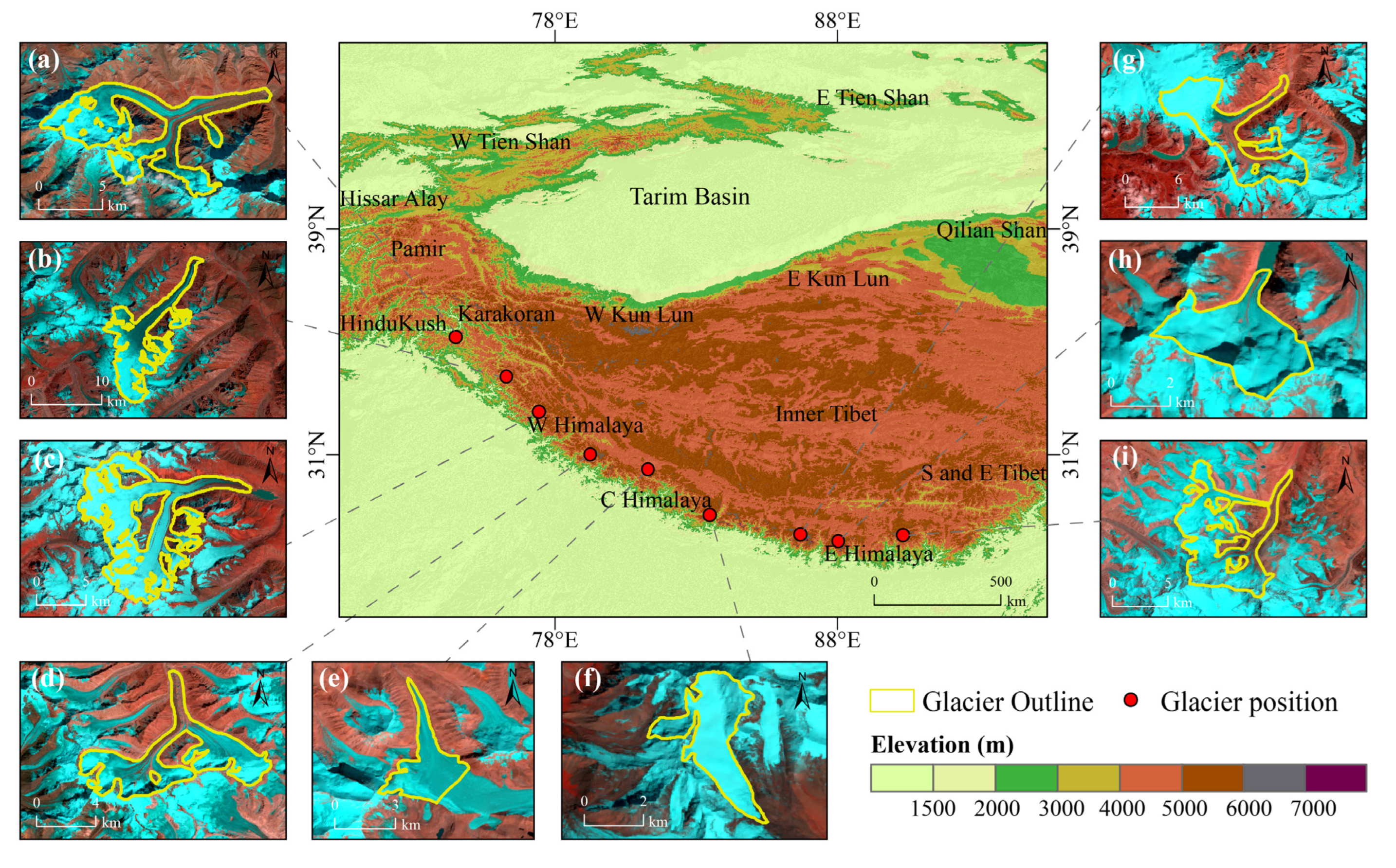
The Himalayas are situated on the southern periphery of the Tibet Plateau, featuring seven of the loftiest summits exceeding an altitude of 8000 m above sea level. This colossal mountain range spans across a distance of 2400 km, with a breadth varying between 150–400 km in an east–west direction. The water reserves stored in the Himalayas glaciers are estimated to be about 1012 m3 [44,45]. To assess the dynamics of mountainous SLA-EMS in the Himalayas, nine glaciers (Figure 1, Table 1) distributed across the west, central, and east Himalayas have been selected for this study. The retreating and thinning of these glaciers have significant implications for agricultural production and geological disasters downstream, and these glaciers’ meltwater is the source of several major rivers [46,47]. The meltwater of Gechongkang, Longbasaba, and Lianggang glacier eventually drain into the Brahmaputra. The Rikha Samba glacier meltwater drains into the Langtang River. The Toshain, Durung Drong, and Samudra Tapu glacier meltwater eventually drain into the Indus. The MaNa and Namunani glacier meltwater eventually drain into the Ganga.
2.2. Data
2.2.1. Landsat Data
This study utilized land surface reflectance data obtained from the Landsat series (TM/ETM+/OLI) during the period from June to September 1991 to 2022. This dataset has a spatial resolution of approximately 30 m and a revisit interval of approximately 16 days. All the land surface reflectance images were radiometrically corrected by the LaSRC [48] (OLI) or LEDAPS [49] (TM/ETM+) atmospheric correction method. That data includes a quality assessment (QA) band, which can identify high-confidence cloud pixels by using CFMask [50,51]. The study used green, near-infrared (NIR), shortwave infrared (SWIR), and QA bands from Landsat image data to extract snow cover, besides using the NIR band to distinguish snow from glaciers. This data can be directly processed and analyzed in GEE by code.
2.2.2. Sentinel-2 MSI
The European Space Agency (ESA) launched the Sentinel-2 satellite in 2017, a multispectral earth observation mission with high spatial and temporal resolutions. It features a high-resolution multi-spectral imager with 13 spectral bands, including 10 m, 20 m, and 60 m spatial resolution, covering a wide swath of 290 km. The satellite’s revisit time is 5 days with two satellites (2A and 2B) at midlatitudes, under cloud-free conditions, providing continuous observation of Earth. The combination of the wide swath and frequent revisit times offered by Sentinel-2 enables continuous monitoring of the Earth’s surface. To validate the SLA-EMS extraction results obtained from Landsat data, the study employed the Sentinel-2 Level-2A product, which is available from GEE.
2.2.3. SRTM DEM and ERA5-LAND Reanalysis
To extract SLA information, the study utilized the SRTM DEM NASA V3.0, acquired from the Shuttle Radar Topography Mission [52]. With a global vertical accuracy of approximately 16 m and a spatial resolution of 30 m, the SRTM DEM NASA V3.0 enabled the study to obtain reliable SLA data. The study also employed ERA5, which provides hourly estimates of atmospheric, land, and oceanic climate variables from 1979 onwards. Due to the complex and rugged topography of the study area, and limited field survey and meteorological data recorded at the meteorological stations, they are not sufficiently representative of the climatic conditions in the study area. We used precipitation/temperature from ERA5 to investigate the relationship between SLA-EMS and meteorology. In addition, compared with other climate reanalysis data, ERA5 has better applicability over the Tibetan Plateau [53,54]. SRTM DEM and ERA5-LAND are available from GEE.
2.2.4. Auxiliary Data
The 2022 Fluctuations of Glaciers database was obtained from the World Glacier Monitoring Service (WGMS, https://wgms.ch/, accessed on 10 December 2022), which collects standardized observations of glacier changes, such as variations in mass, volume, area, and length, over time. The WGMS employs the Fluctuations of Glaciers methodology for this purpose. In addition, the study used version 6.0 of the Randolph Glacier Inventory (RGI 6.0), which contains digital outlines of glaciers worldwide, sourced from the Global Land Ice Measurements from Space initiative [55]. To analyze the influence of the El Niño/Southern Oscillation on glacier fluctuations, the study employed the bi-monthly multivariate El Niño/Southern Oscillation (MEI.v2, https://psl.noaa.gov/enso/mei/, accessed on 10 February 2023) index [56,57]. The MEI.v2 is a time series of the dominant combined empirical orthogonal function of five variables, namely sea level pressure, sea surface temperature, zonal and meridional components of the surface wind, and outgoing longwave radiation, over the tropical Pacific basin.
3. Methods
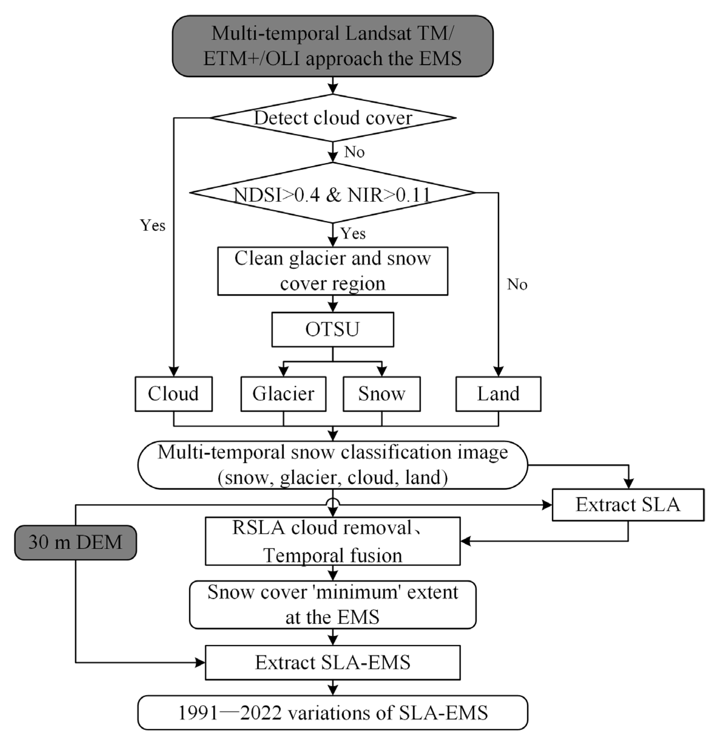
The complete flowchart outlining the process of extracting SLA-EMS is illustrated in Figure 2. The methodology can be categorized into three key phases: (1) SNOMAP and OTSU thresholding algorithm for snow classification map (snow, glacier, land, cloud), (2) minimize snow cover extraction at the end of the melting season, and (3) regional SLA extraction and accuracy verification.
3.1. Snow Mapping
The QA band was used to identify Landsat images data clouds and eliminate cloud pixels. After excluding cloud cover, the SNOMAP algorithm was employed in this study for snow classification, leveraging the pronounced spectral difference between the shortwave infrared (SWIR) and visible bands. This algorithm is the most commonly used in snow and glacier remote sensing [58,59]. We take advantage of these bands’ features to establish a computationally efficient method for mapping clean glacier and snow areas using the normalized difference snow index (NDSI). The NDSI is calculated according to the equation:
where ρGreen is the surface reflectance in the green band and ρSWIR is the surface reflectance in the SWIR band. Furthermore, in order to mitigate the effects of water and mountain shadows, this algorithm utilizes only the reflectance values of NIR greater than 0.11. The specific strategy is that a pixel with NDSI > 0.4 and NIR > 0.11 is identified as the clean glacier and snow pixels.
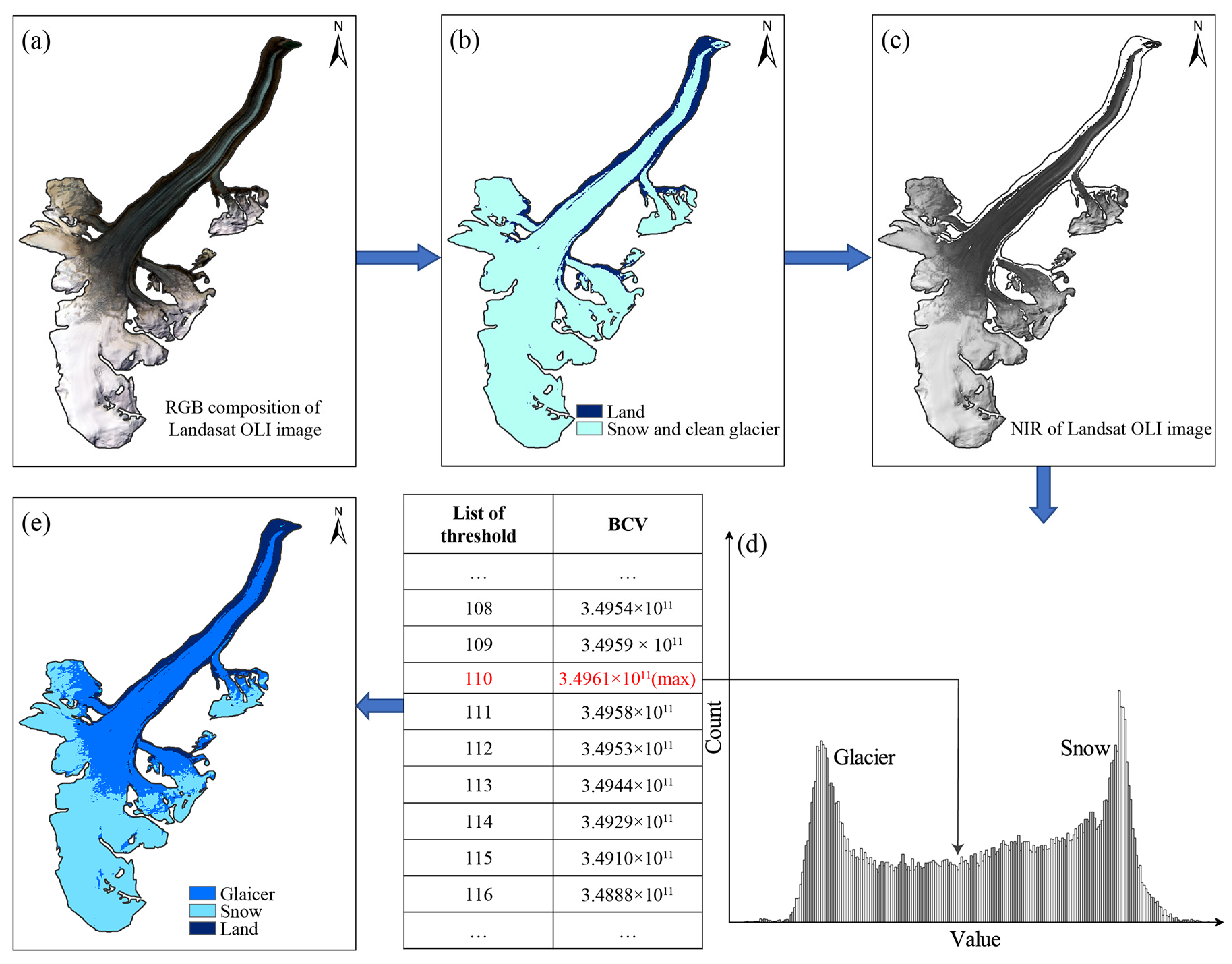
The OTSU thresholding method [60] is an adaptive technique used for image segmentation. In this study, it is used for distinguishing between ice and snow [61,62]. Moreover, this technique is well-suited for delimiting snowlines for a vast number of glaciers, in comparison to manual interpretation and semi-automated methods [63]. The method utilized in this study is based on the principle that the gray-level which maximizes the between-class variance (BCV) is chosen as the threshold, which maximizes the separability function between two classes. (Figure 3). In this study, we utilized the distinct NIR spectral reflection characteristics of the clean glacier and snow to apply threshold functions that enabled the separation of the two. The use of NIR in this way facilitated the differentiation of glaciers and snow in the imagery. Additionally, a snow classification image is obtained by combining the identified snow, glacier, land, and the identified cloud in the QA band.
3.2. Snow Cover Minimum Extent Extraction
The cloud removal and time series fusion are carried out through the transient SLA to reduce the impact of clouds and obtain the most appropriate minimum snow cover range at the end of the melting season.
3.2.1. Transient Snowline Altitude Cloud Removal
To determine the ratio of snow cover to cloud cover in the area, we judge that if the proportion of cloud cover and snow cover was less than 1, the transient regional SLA (Section 3.3) of the area would be extracted to remove the clouds. The strategy of transient SLA cloud removal: if the height of a pixel classified as a cloud was higher than the instantaneous SLA, it would be categorized as snow. Conversely, if it was lower than the instantaneous SLA, it would be categorized as land. When the proportion of cloud cover is too large, it is easy to have very few snow pixels or cloud cover all around the snow cover area, which results in a large deviation or unable to extract the transient SLA. To ensure the efficacy of the extracted transient SLA, this study sets that when the ratio of cloud to snow area is greater than 1, it will directly participate in the temporal fusion processing.
3.2.2. Time Series Fusion
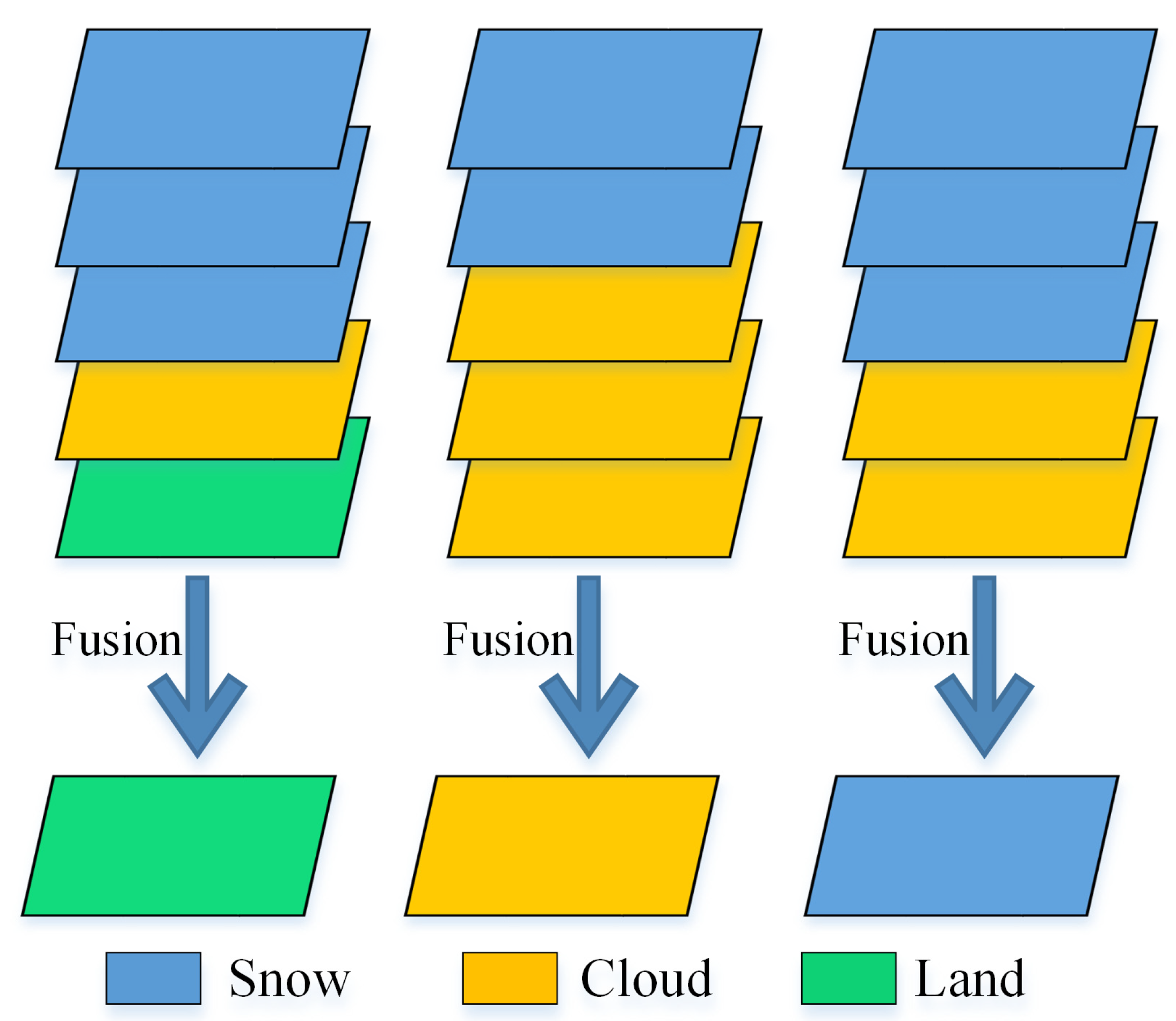
The time series fusion using multi-temporal snow classification images (including images after cloud removal of transient SLA) approaches the end of the snowmelt season. We obtain the map of the minimum snow cover that represents the end of the snowmelt season. The strategy of time series fusion is as follows: each pixel is classified as land if it is distinguished as land by any temporal phase. When over 50% of the pixel are identified as snow and other time series are classified as clouds, the pixel is labeled as snow. Conversely, when more than 50% of the pixel are identified as clouds and other time series are labeled as snow, the pixel is classified as clouds (Figure 4). The minimum snow coverage map representing the end of the snowmelt season obtained after fusion is used to extract the SLA-EMS.
3.3. Regional Snowline Altitude Extraction
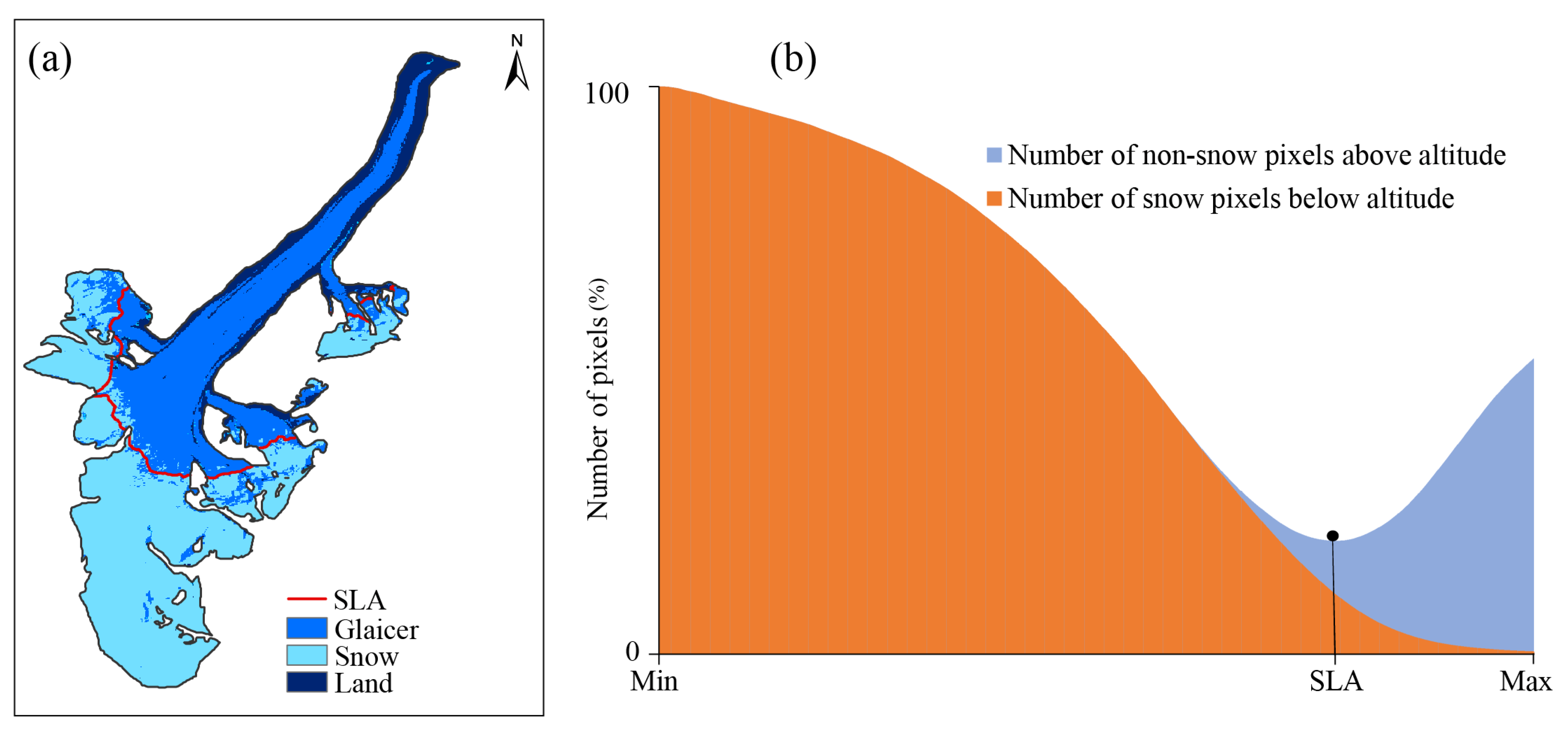
Our study presents a method for extracting regional SLA based on the approach developed by Krajčí et al. (2014) [5]. The proposed method is based on the principle of determining an altitude within the target region that minimizes the sum of non-snow pixels above the altitude and snow pixels below the altitude. The altitude corresponding to this condition is considered to represent the SLA in the region (Figure 5). The calculation of regional SLA is expressed as:
where sum is the total of the number of snow pixels below the altitude (Cbelow) and the number of non-snow pixels above the altitude (Cabove), elevmin is the minimum altitude in the region, and elevmax is the maximum altitude in the region.
The specific process starts from the minimum altitude of the region and calculates the total of the number of snow pixels below the target altitude and the number of non-snow pixels above the altitude. Then, the calculation is carried out once for every additional 1 m altitude to the maximum altitude in the region. Finally, find the minimum value sumSLA and the altitude corresponding to this value is the SLA in this region. This method can allow the existence of partial cloud coverage and is the optimal estimation of SLA in the target region. This method is used to extract transient SLA and SLA-EMS.
3.4. Accuracy Assessment
The Sentinel-2 image with higher spatial resolution and shorter revisit period is used to verify the accuracy of the Landsat data in extracting the SLA-EMS by extracting the minimum snow cover range at the end of the melting season. The specific verification method is as follows: for snow cover mapping using the visual interpretation method, multi-temporal Sentinel-2 remote sensing images of each scene, approaching the end of snowmelt season and with cloud cover less than 10% in the study area, from 2019 to 2022 have been utilized. Then, these images adopt the same time series fusion strategy with Landsat to obtain the minimum snow cover range at the end of the melting season extracted by Sentinel-2, and the image is taken as the true value. Finally, based on the minimum snow cover range map at the end of the melting season extracted by Sentinel-2, random sampling of verification samples is conducted near the snowline location, and combined with DEM data and the SLA-EMS extracted by Landsat, to calculate the overall accuracy (OA), precision (Pre), recall (Rec), and kappa coefficient of the SLA-EMS extraction model. The calculation is expressed as:
where A is the number of points above the SLA-EMS of the Landsat and identified as snow in the Sentinel-2 minimum snow coverage, B is the number of points above the SLA-EMS of the Landsat and identified as snow-free in the Sentinel-2 minimum snow coverage, C is the number of points below the SLA-EMS of the Landsat and identified as snow in the Sentinel-2 minimum snow coverage, and D is the number of points below the SLA-EMS of the Landsat and identified as snow-free in the Sentinel-2 minimum snow coverage. When the Pre > Rec, there is an overestimation of SLA, when the Pre < Rec, there is an underestimate of the SLA.
4. Results
4.1. Accuracy of SLA-EMS
The accuracy of the SLA-EMS extraction in the study areas based on Landsat was evaluated quantitatively by establishing a confusion matrix and calculating the OA, Pre, Rec, and Kappa coefficients (Table 2). The results show that the extraction of SLA-EMS in the study area has high accuracy. OA is 92.6%, and the Kappa coefficient is 0.85. However, the Pre in the study area is slightly lower than Rec, indicating that the SLA-EMS extracted by Landsat is slightly underestimated compared with the minimum snow cover range at the end of the melting season at Sentinel-2 with higher time resolution. The Pre of the study area is 90.9%, which means that the probability of being identified as snow-free cover in the minimum snow cover range extracted by Sentinel-2 above the SLA-EMS period extracted by Landsat is 9.1%. The Rec of the study area is 94.9%, which means that the probability of being identified as snow cover in the minimum snow cover range extracted by Sentinel-2 under the SLA-EMS extracted by Landsat is only 5.1%.
4.2. Regional SLA Dynamics during the Snowmelt Season
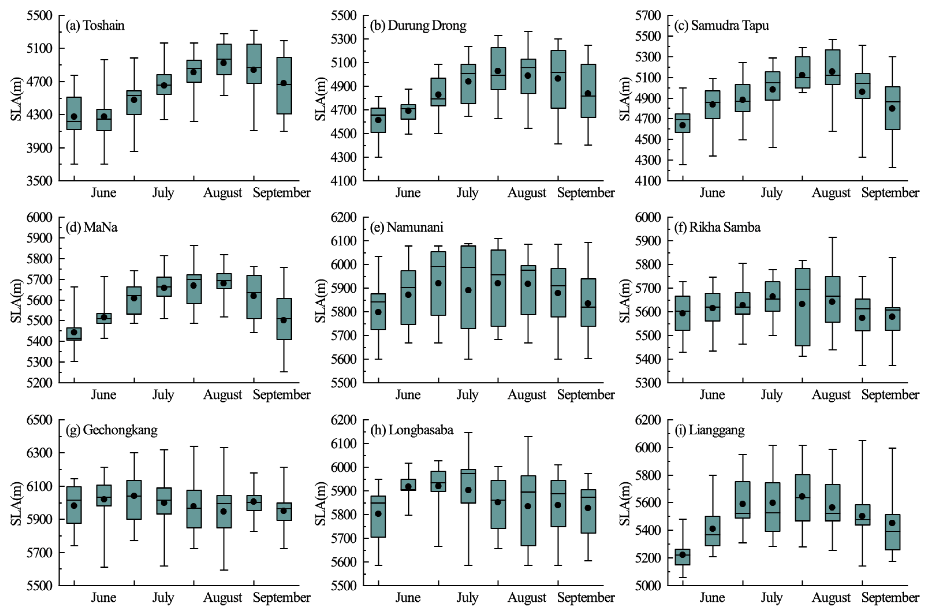
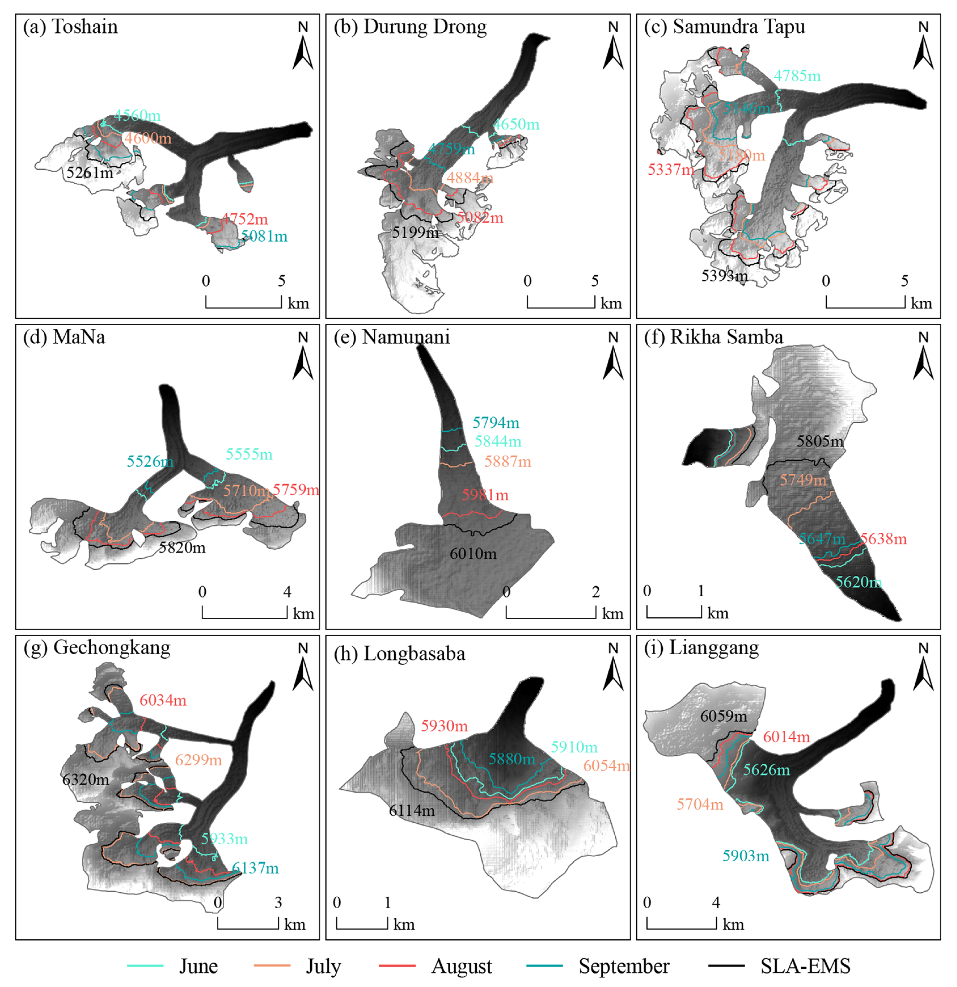
The time series of regional SLA for different glaciers from June to September at 16 days intervals are demonstrated in Figure 6. The regional SLA gradually increases from June onwards due to the snowpack melting, reaching its maximum in July or August, and subsequently decreasing thereafter. The regional SLA exhibits large interannual fluctuations, which differ in different glaciers. To further visualize the regional SLA dynamics during the snowmelt season, Figure 7 displays the spatial pattern of the regional SLA for different glaciers (the black line indicates the SLA-EMS). Overall, the glaciers located in the East Himalayas have the highest Regional SLA, while the West Himalayas has a lower regional SLA. The regional SLA during the snowmelt season and the SLA-EMS reflect well the snow cover state of retreat above the glacier area. Taking Durung Drong as an example, the regional SLA rises from 4650 m (June) to 5082 m (August) and declines to 4759 m (September). Additionally, the SLA-EMS (5199 m) is higher than all the regional SLAs during the snowmelt season, reaching the peak of snow cover retreat.
4.3. Interannual Variations of SLA-EMS
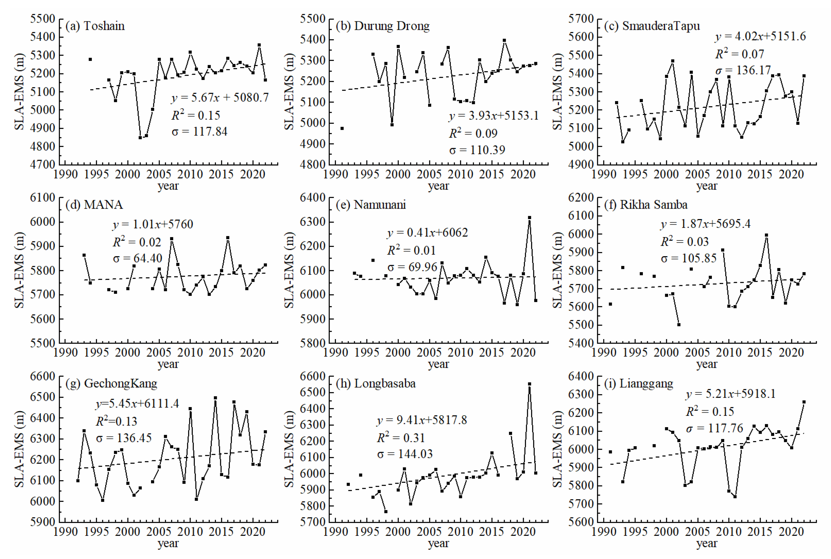
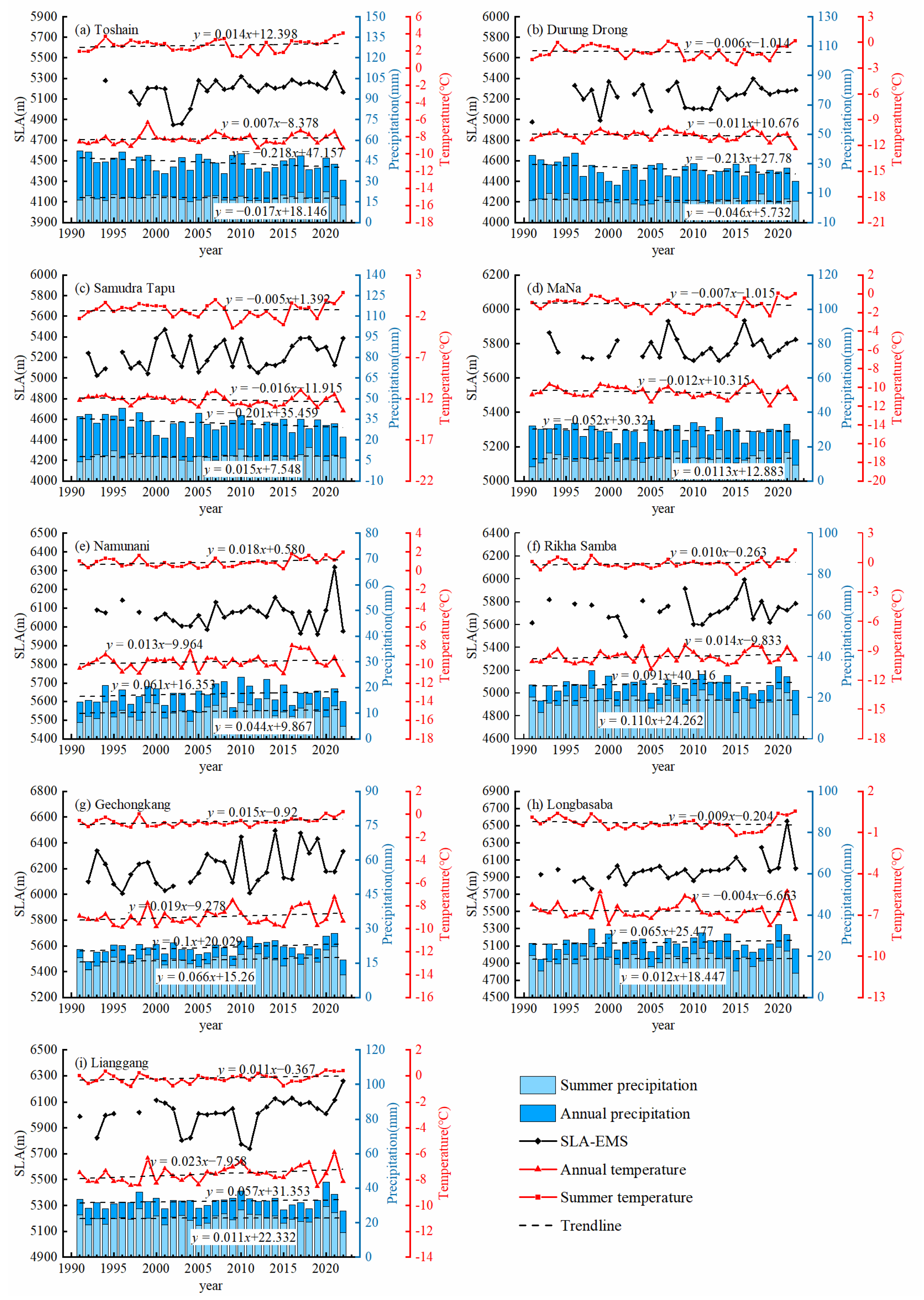
To illustrate the fluctuations of snow cover at the end of the melting season, the interannual variations of SLA-EMS are presented in Figure 8. Overall, the mean SLA-EMS gradually increases from the West Himalaya to the East Himalaya, from Toshain (5188 m) to GechongKang (6204 m). The SLA-EMS for all glaciers generally shows an increasing trend during 1991–2022, ranging from about 13 to 301 m. Specifically, the SLA-EMS of Longbasaba is the significantly fastest rising (linear trend = 9.41 m·a−1, p < 0.05), increasing by approximately 200.4 m. The SLA-EMS of Namunani is the slowest rising (linear trend = 0.4 m·a−1), increased by approximately 13 m. In addition, the standard deviation (σ) reflects the interannual fluctuations of SLA-EMS. It can be seen that MaNa shows a relatively low standard deviation of SLA-EMS (σ = 64.4 m) reflecting the small interannual variability. Longbasaba shows relatively high interannual variability of SLA-EMS (σ = 144.03 m), reflecting its unstable snow cover state.
4.4. The Influences of Climate Factors on SLA-EMS
Figure 9 shows the interannual variations of annual temperature/precipitation and summer temperature/precipitation. The annual temperature/precipitation refers to the mean temperature/total precipitation from the previous year October to the current year September and the summer temperature/precipitation refers to the mean temperature/total precipitation during the current year June–August. The temperatures of Durung Drong, Samudra Tapu, MaNa, and Longbasaba have exhibited a declining trend over the past three decades. Similarly, the yearly precipitation in the three glacial regions situated in the Western Himalayas Mountains has displayed a conspicuous downward trend. The Rikha Samba, GechongKang, Longbasaba, and Lianggang precipitation in the central and eastern Himalayas are mainly concentrated in summer, and the summer precipitation accounts for 70.2%, 75.4%, 70.2%, and 69.7% of the whole year, respectively. Toshain has the highest average summer temperature (2.6 °C), and Longbasaba has had the highest average annual temperature (−6.7 °C) over the past three decades. Samudra Tapu has had the lowest average summer (−1.3 °C) and annual (−12.2 °C) temperature over the past three decades. Figure 9 shows that some correlation between temperature and SLA-EMS. For instance, both the temperature and SLA-EMS of MaNa reached a maximum in 2008, reached a minimum in 2019.
Table 3 further displays the correlation of the SLA-EMS, annual temperature/precipitation, and summer temperature/precipitation for different glaciers. The correlation between SLA-EMS and temperature is typically positive, while it is negative with precipitation for almost all glaciers. This implies that SLA-EMS would increase with temperature rise or precipitation decline. More specifically, the SLA-EMS correlates more with precipitation than the temperature for Durung Drong, Samudra Tapu, Namunani, Rikha Samba, and Lianggang. Among them, the SLA-EMS is significantly affected by annual precipitation in Durung Drong (p < 0.05) and Samudra Tapu (p < 0.01), while it is significantly affected by summer precipitation in Lianggang (p < 0.01). The SLA-EMS correlates more with temperature than precipitation for Toshain, MaNa, Gechongkang, and Longbasaba. Among them, the SLA-EMS is significantly affected by annual temperature in MaNa (p < 0.01) and Longbasaba (p < 0.01), while it is significantly affected by summer temperature in Gechongkang (p < 0.05).
5. Discussion
5.1. Uncertainties and Limitations
In this study, we present a method approach to extract the SLA-EMS by utilizing long-term (1991–2022) continuous Landsat observations developed to track the dynamics of SLA-EMS in the Himalayas. The SLA-EMS extracted by this method can capture the snow cover state above the nine glacier areas with relatively high accuracy (Section 4.1 and Section 4.2). However, the uncertainties and limitations (including snow cover mapping and SLA-EMS extraction) may come from the following:
- (1)
- in mountainous regions, the accuracy of snow cover range extraction using optical remote sensing images can be influenced by topographic effects, such as mountain shadows caused by terrain fluctuations (topographic effect). The topographic effect had a significant impact on the progress of remote sensing in mountainous regions [64,65], and thus many researchers have developed topographic correction methods. For instance, the spectral reflectance of snow cover is reduced in mountainous areas under the shadow, as compared to the reflectance of soil or vegetation that is exposed to direct sunlight. The latest topographic correction methods may greatly eliminate the effect of topographic effect on mountain snow cover information identification [66,67,68]. In addition, for the SLA extraction at the pixel scale [4,35], the effect of microtopographic factors (e.g., slope gradients and aspect) on SLA should be considered. This study focuses on the SLA at the regional scale (e.g., a glacier area or a catchment) to obtain one comprehensive SLA value for a region. Therefore, this study does not consider the slight effect of the topographic effect and microtopographic factors for a while.
- (2)
- cloud and cloud shadow interferences have long been one of the most significant error sources of snow cover information extraction in optical remote sensing. In this study, a small amount of cloud cover can be removed by the regional SLA (when the proportion of cloud cover and snow cover is less than 1). However, when this ratio is greater than 1 (very large), the accuracy of the extracted regional SLA is greatly reduced, and then so is the accuracy of cloud removal. Moreover, the cloud information of Landsat is derived from the cloud flag based on the CFMask algorithm with an overall accuracy of 96.4% [69]. Selkowitz et al. [70] (2015) reported that the CFMask algorithm was susceptible to commission errors in regions of rocky, alpine terrain, and where a combination of snow, ice, and other land cover types were present. In this case, the revised CFmask approach developed by Selkowitz et al. (2015) can be adopted to improve the ability of cloud recognition based on Landsat data. Additionally, combining Sentinel-1 synthetic aperture radar (SAR) remote sensing data with Sentinel-2 optical remote sensing data can improve the ability to identify snow cover under cloud cover [71,72].
- (3)
- Landsat image has a long revisit period (16 days) and there are inevitable data gaps at a certain time, originating from cloud cover, sensor, orbital limitations, and other factors. In this case, the available snow cover maps during the snowmelt season are quite scarce, and thus the accuracy of SLA-EMS extraction will be affected.
5.2. Spatiotemporal Variation of SLA-EMS
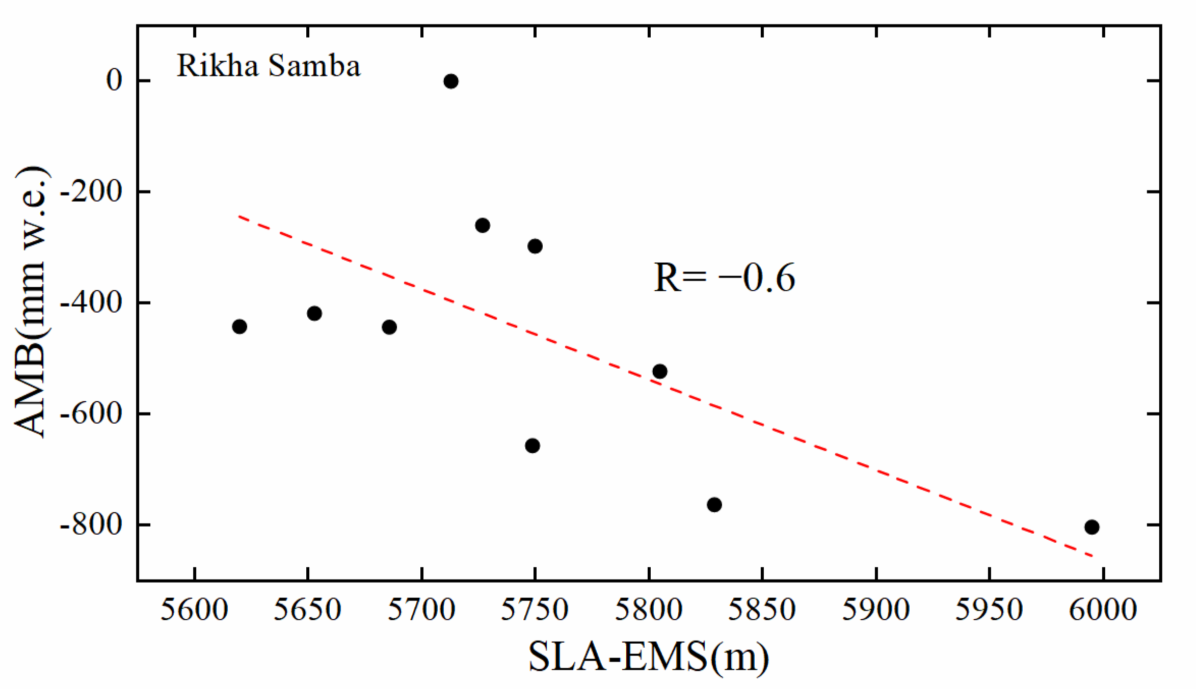
This study found that spatial interannual fluctuation of the SLA-EMS in the study areas had shown an upward trend in the past three decades (Figure 8), which is very in keep with the research conclusion that the material balance of Himalayas Mountain is in a negative balance state [21,25,73,74]. Previous studies, such as Maanya et al. (2016) [75] and Wei et al. (2021) [76], have documented the rapid retreat and fragmentation of Durung Drong and Longbasaba glaciers, which corresponds with the observed increase in SLA-EMS of both glaciers in our study. Furthermore, we conducted the correlation between the annual mass balance (AMB) of Rikha Samba in 11 years and its corresponding SLA-EMS was analyzed (as shown in Figure 10), revealing a considerable negative correlation between the two variables. The methodology developed in this study is anticipated to enhance the precision of assessing the annual mass balance of glaciers and offer essential data support for reconstructing long-term, large-scale annual mass balance.
The SLA-EMS in the western Himalayas is the lowest, and the SLA-EMS in the eastern Himalayas is the highest. The observed spatial pattern in the distribution of SLA could be explained by the fact that the Eastern Himalayas have higher elevations than the West Himalayas. The average altitude of the three study areas in the Eastern Himalayas is approximately 6067 m, while that of the West Himalayas is about 5212 m. The distribution pattern of SLA-EMS, which is influenced by topographic height, can be explained by the mass altitude effect. This effect is caused by the thermodynamic impact of mountainous masses [77]. Besides, we found that the overall SLA-EMS of Namunani on the northern slope is higher than that of Rikha Samba on the southern slope of the central Himalayas. Additionally, some studies have shown that the SLA of the Himalayas is low on the south slope and high on the north slope [78,79]. The reason is that the south slope of the Himalayas has a monsoon climate with high temperatures and distinct dry and rainy seasons. Precipitation increases in summer under the influence of the Indian monsoon. Precipitation decreases in winter while it decreases in the north slope in a high and cold climate. The terrain of the high Himalayas obstructs not only the cold air from the north to the southern slope but also the significant amount of water vapor carried by the Indian monsoon from the southern slope to the northern slope, resulting in a notable decrease in water vapor reaching the northern slope. This phenomenon leads to a significant difference in SLA between the southern and northern slopes, with the SLA on the southern slope being lower than that on the northern slope.
5.3. Effect of Climatic Factors and ENSO on SLA-EMS
As a kind of climate marker line, the altitude of the snowline is affected by climate factors and also reflects climate change. The existing research shows that under the influence of global warming, the glacier area is shrinking, and the SLA is increasing [4], which is consistent with the research in this paper. The study found that SLA-EMS in different regions of the Himalayas in a W-E direction have different sensitivity to precipitation and temperature. There exists a positive correlation between SLA and temperature, such that an increase in temperature leads to an increase in SLA. Conversely, there is a negative correlation between SLA and precipitation, such that increased precipitation results in a decrease in SLA.
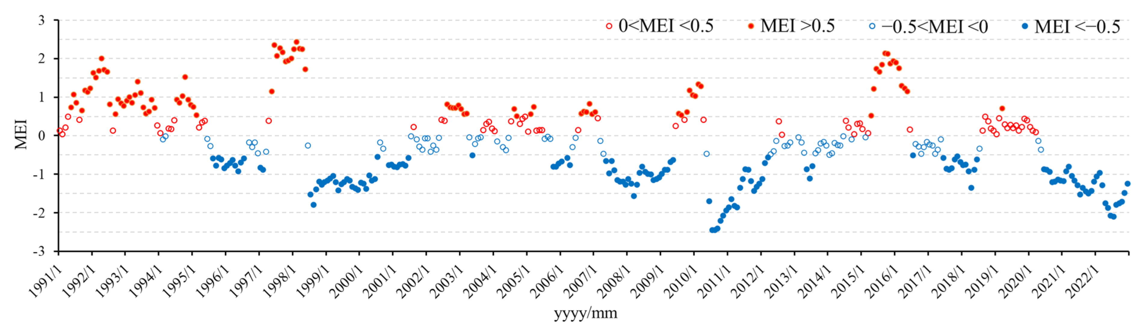
The variation of SLA is closely related to atmospheric circulation. When abnormal changes in atmospheric circulation occur, the extreme climate will occur and the SLA will be abnormal [80]. ENSO is the most typical strong signal of global air–sea interaction, which has a great influence on the interannual variation of SLA control [81]. Figure 11 shows the statistics of warm and cold periods in ENSO from 1991 to 2022. Obviously, the MEI from 2007 to early 2009 and from early 2010 to early 2012 continued to be less than 0, experiencing a long cold period, the SLA-EMS of Durung Drong, MaNa, Rikha Samba, Longbasaba, and Lianggang showed troughs during this period (Figure 8). Additionally, the MEI from 2015 to early 2016 was greater than 0, experiencing a warm period, the SLA-EMS in glaciers such as MaNa and Lianggang showed peaks during this period (Figure 8). Therefore, it is inferred that the abnormal SLA-EMS variation of the Himalayas glacier may be due to the action of La Niña and El Niño through global air–sea.
6. Conclusions
Comprehending the dynamics of SLA-EMS is crucial in signifying the impact of climate change. The main goal of this research is to establish a dataset of SLA-EMS (1991–2022) for nine glacier regions in the Himalayas, employing the newly developed method for extracting SLA-EMS. On this basis, the spatiotemporal dynamics of SLA-EMS and their relationship to meteorological factors (temperature/precipitation) are analyzed. The primary findings can be condensed as follows:
- (1)
- The developed method for extracting the spatiotemporal patterns of the snowline altitude at the end of the melting season (SLA-EMS) is efficient. Furthermore, the accuracy of the extracted SLA-EMS data was assessed using higher resolution Sentinel-2 data, resulting in an OA of 92.6% and a Kappa coefficient of 0.85.
- (2)
- The SLA-EMS in all glacier areas in the Himalayas exhibited a general increasing trend during the period from 1991 to 2022. The SLA-EMS of Longbasaba is the significantly fastest rising (9.41 m·a−1), and the SLA-EMS of Namunani is the slowest rising (0.4 m·a−1).
- (3)
- The results of the correlation analyses between the SLA-EMS and temperature/precipitation demonstrate that the sensitivity of temperature and precipitation to variations in SLA-EMS varies across the different glacier areas. However, annual temperature/precipitation has a more significant impact than summer temperature/precipitation in general. The atmospheric circulation might have also been associated with anomalous SLA-EMS.
- (4)
- The robust storage and computational capabilities of the GEE platform have significantly enhanced the efficiency of remote sensing-based SLA extraction and provided substantial computational resources for large-scale and long-term monitoring of SLA dynamics.
Author Contributions
Conceptualization, Z.T. and J.W.; writing—original draft preparation, J.W.; writing—review and editing, Z.T. and G.D.; supervision, Z.T.; validation, G.H., Y.Y. and Y.Z.; funding acquisition, Z.T. All authors have read and agreed to the published version of the manuscript.
Funding
This research was funded by the Science and Technology Innovation Program of Hunan Province, China (Grant No. 2022RC1240), the National Natural Science Foundation of China (Grant No. 41871058), and the State Key Laboratory of Cryospheric Science, Northwest Institute of Eco-Environment and Resources, Chinese Academy Sciences (Grant No. SKLCS-OP-2020-08).
Data Availability Statement
Data sharing is not applicable.
Acknowledgments
We thank the USGS and Google for the use of available satellite imagery. We would like to thank the editors and anonymous reviewers for their helpful comments and constructive suggestions.
Conflicts of Interest
The authors declare no conflict of interest.
References
- Barnett, T.P.; Adam, J.C.; Lettenmaier, D.P. Potential impacts of a warming climate on water availability in snow-dominated regions. Nature 2005, 438, 303–309. [Google Scholar] [CrossRef] [PubMed]
- Tang, Z.; Wang, X.; Wang, J.; Wang, X.; Li, H.; Jiang, Z. Spatiotemporal variation of snow cover in Tianshan Mountains, Central Asia, based on cloud-free MODIS fractional snow cover product, 2001–2015. Remote Sens. 2017, 9, 1045. [Google Scholar] [CrossRef]
- Bormann, K.J.; Brown, R.D.; Derksen, C.; Painter, T.H. Estimating snow-cover trends from space. Nat. Clim. Chang. 2018, 8, 924–928. [Google Scholar] [CrossRef]
- Deng, G.; Tang, Z.; Hu, G.; Wang, J.; Sang, G.; Li, J. Spatiotemporal dynamics of snowline altitude and their responses to climate change in the Tienshan Mountains, Central Asia, During 2001–2019. Sustainability 2021, 13, 3992. [Google Scholar] [CrossRef]
- Krajčí, P.; Holko, L.; Perdigão, R.A.; Parajka, J. Estimation of regional snowline elevation (RSLE) from MODIS images for seasonally snow covered mountain basins. J. Hydrol. 2014, 519, 1769–1778. [Google Scholar] [CrossRef]
- Girona-Mata, M.; Miles, E.S.; Ragettli, S.; Pellicciotti, F. High-resolution snowline delineation from Landsat imagery to infer snow cover controls in a Himalayan catchment. Water Resour. Res. 2019, 55, 6754–6772. [Google Scholar] [CrossRef]
- Lorrey, A.M.; Vargo, L.; Purdie, H.; Anderson, B.; Cullen, N.J.; Sirguey, P.; Mackintosh, A.; Willsman, A.; Macara, G.; Chinn, W. Southern Alps equilibrium line altitudes: Four decades of observations show coherent glacier–climate responses and a rising snowline trend. J. Glaciol. 2022, 68, 1127–1140. [Google Scholar] [CrossRef]
- Baum, S.K.; Crowley, T.J. Seasonal snowline instability in a climate model with realistic geography: Application to carboniferous (~300 MA) glaciation. Geophys. Res. Lett. 1991, 18, 1719–1722. [Google Scholar] [CrossRef]
- Mengel, J.; Short, D.; North, G. Seasonal snowline instability in an energy balance model. Clim. Dyn. 1988, 2, 127–131. [Google Scholar] [CrossRef]
- Østrem, G. The transient snowline and glacier mass balance in southern British Columbia and Alberta, Canada. Geogr. Ann. Ser. A Phys. Geogr. 1973, 55, 93–106. [Google Scholar] [CrossRef]
- Mernild, S.H.; Pelto, M.; Malmros, J.K.; Yde, J.C.; Knudsen, N.T.; Hanna, E. Identification of snow ablation rate, ELA, AAR and net mass balance using transient snowline variations on two Arctic glaciers. J. Glaciol. 2013, 59, 649–659. [Google Scholar] [CrossRef]
- Pandey, P.; Kulkarni, A.V.; Venkataraman, G. Remote sensing study of snowline altitude at the end of melting season, Chandra-Bhaga basin, Himachal Pradesh, 1980–2007. Geocarto Int. 2013, 28, 311–322. [Google Scholar] [CrossRef]
- Tang, Z.; Wang, X.; Deng, G.; Wang, X.; Jiang, Z.; Sang, G. Spatiotemporal variation of snowline altitude at the end of melting season across High Mountain Asia, using MODIS snow cover product. J. Appl. Remote Sens. 2020, 66, 2629–2645. [Google Scholar] [CrossRef]
- Qin, D.; Yao, T.; Ding, Y. Glossary of Cryospheric Science; China Meteorological Press: Beijing, China, 2014; pp. 158–159. [Google Scholar]
- Rabatel, A.; Bermejo, A.; Loarte, E.; Soruco, A.; Gomez, J.; Leonardini, G.; Vincent, C.; Sicart, J.E. Can the snowline be used as an indicator of the equilibrium line and mass balance for glaciers in the outer tropics? J. Glaciol. 2012, 58, 1027–1036. [Google Scholar] [CrossRef]
- Shea, J.; Menounos, B.; Moore, R.; Tennant, C. An approach to derive regional snow lines and glacier mass change from MODIS imagery, western North America. Cryosphere 2013, 7, 667–680. [Google Scholar] [CrossRef]
- Barandun, M.; Huss, M.; Usubaliev, R.; Azisov, E.; Berthier, E.; Kääb, A.; Bolch, T.; Hoelzle, M. Multi-decadal mass balance series of three Kyrgyz glaciers inferred from modelling constrained with repeated snow line observations. Cryosphere 2018, 12, 1899–1919. [Google Scholar] [CrossRef]
- McFadden, E.; Ramage, J.; Rodbell, D. Landsat TM and ETM+ derived snowline altitudes in the Cordillera Huayhuash and Cordillera Raura, Peru, 1986–2005. Cryosphere 2011, 5, 419–430. [Google Scholar] [CrossRef]
- You, Q.; Wu, T.; Shen, L.; Pepin, N.; Zhang, L.; Jiang, Z.; Wu, Z.; Kang, S.; AghaKouchak, A. Review of snow cover variation over the Tibetan Plateau and its influence on the broad climate system. Earth Sci. Rev. 2020, 201, 103043. [Google Scholar] [CrossRef]
- Tang, Z.; Ma, J.; Peng, H.; Wang, S.; Wei, J. Spatiotemporal changes of vegetation and their responses to temperature and precipitation in upper Shiyang river basin. Adv. Space Res. 2017, 60, 969–979. [Google Scholar] [CrossRef]
- Kehrwald, N.M.; Thompson, L.G.; Tandong, Y.; Mosley-Thompson, E.; Schotterer, U.; Alfimov, V.; Beer, J.; Eikenberg, J.; Davis, M.E. Mass loss on Himalayan glacier endangers water resources. Geophys. Res. Lett. 2008, 35, L22503. [Google Scholar] [CrossRef]
- Mayewski, P.A.; Jeschke, P.A. Himalayan and Trans-Himalayan glacier fluctuations since AD 1812. Arct. Alp. Res. 1979, 11, 267–287. [Google Scholar] [CrossRef]
- Bahuguna, I.; Rathore, B.; Brahmbhatt, R.; Sharma, M.; Dhar, S.; Randhawa, S.; Kumar, K.; Romshoo, S.; Shah, R.; Ganjoo, R. Are the Himalayan glaciers retreating? Curr. Sci. 2014, 106, 1008–1013. [Google Scholar]
- Lee, E.; Carrivick, J.L.; Quincey, D.J.; Cook, S.J.; James, W.H.; Brown, L.E. Accelerated mass loss of Himalayan glaciers since the Little Ice Age. Sci. Rep. 2021, 11, 24284. [Google Scholar] [CrossRef]
- Kulkarni, A.V.; Karyakarte, Y. Observed changes in Himalayan glaciers. Curr. Sci. 2014, 106, 237–244. [Google Scholar]
- Guo, H.; Li, X.; Qiu, Y. Comparison of global change at the Earth’s three poles using spaceborne Earth observation. Chin. Sci. Bull. 2020, 65, 1320–1323. [Google Scholar] [CrossRef]
- Gascoin, S.; Grizonnet, M.; Bouchet, M.; Salgues, G.; Hagolle, O. Theia Snow collection: High-resolution operational snow cover maps from Sentinel-2 and Landsat-8 data. Earth Syst. Sci. Data 2019, 11, 493–514. [Google Scholar] [CrossRef]
- Debnath, M.; Sharma, M.C.; Syiemlieh, H.J. Glacier dynamics in changme khangpu basin, sikkim himalaya, India, between 1975 and 2016. Geosciences 2019, 9, 259. [Google Scholar] [CrossRef]
- Ran, Y.; Li, X.; Cheng, G.; Nan, Z.; Che, J.; Sheng, Y.; Wu, Q.; Jin, H.; Luo, D.; Tang, Z. Mapping the permafrost stability on the Tibetan Plateau for 2005–2015. Sci. China Earth Sci. 2021, 64, 62–79. [Google Scholar] [CrossRef]
- Guo, W.; Liu, S.; Xu, J.; Wu, L.; Shangguan, D.; Yao, X.; Wei, J.; Bao, W.; Yu, P.; Liu, Q. The second Chinese glacier inventory: Data, methods and results. J. Glaciol. 2015, 61, 357–372. [Google Scholar] [CrossRef]
- Tang, Z.; Deng, G.; Hu, G.; Zhang, H.; Pan, H.; Sang, G. Satellite observed spatiotemporal variability of snow cover and snow phenology over high mountain Asia from 2002 to 2021. J. Hydrol. 2022, 613, 128438. [Google Scholar] [CrossRef]
- Choubin, B.; Alamdarloo, E.H.; Mosavi, A.; Hosseini, F.S.; Ahmad, S.; Goodarzi, M.; Shamshirband, S. Spatiotemporal dynamics assessment of snow cover to infer snowline elevation mobility in the mountainous regions. Cold Reg. Sci. Technol. 2019, 167, 102870. [Google Scholar] [CrossRef]
- Notarnicola, C. Hotspots of snow cover changes in global mountain regions over 2000–2018. Remote Sens. Environ. 2020, 243, 111781. [Google Scholar] [CrossRef]
- Verbyla, D.; Hegel, T.; Nolin, A.W.; Van de Kerk, M.; Kurkowski, T.A.; Prugh, L.R. Remote sensing of 2000–2016 alpine spring snowline elevation in dall sheep mountain ranges of Alaska and Western Canada. Remote Sens. 2017, 9, 1157. [Google Scholar] [CrossRef]
- Spiess, M.; Huintjes, E.; Schneider, C. Comparison of modelled-and remote sensing-derived daily snow line altitudes at Ulugh Muztagh, northern Tibetan Plateau. J. Mt. Sci. 2016, 13, 593–613. [Google Scholar] [CrossRef]
- Tang, Z.; Wang, J.; Li, H.; Liang, J.; Li, C.; Wang, X. Extraction and assessment of snowline altitude over the Tibetan plateau using MODIS fractional snow cover data (2001 to 2013). J. Appl. Remote Sens. 2014, 8, 084689. [Google Scholar] [CrossRef]
- Hu, Z.; Dietz, A.; Kuenzer, C. The potential of retrieving snow line dynamics from Landsat during the end of the ablation seasons between 1982 and 2017 in European mountains. Int. J. Appl. Earth Obs. Geoinf. 2019, 78, 138–148. [Google Scholar] [CrossRef]
- Guo, Z.; Wang, N.; Wu, H.; Wu, Y.; Wu, X.; Li, Q. Variations in firn line altitude and firn zone area on Qiyi Glacier, Qilian Mountains, over the period of 1990 to 2011. Arct. Antarct. Alp. Res. 2015, 47, 293–300. [Google Scholar] [CrossRef]
- Gorelick, N.; Hancher, M.; Dixon, M.; Ilyushchenko, S.; Thau, D.; Moore, R. Google Earth Engine: Planetary-scale geospatial analysis for everyone. Remote Sens. Environ. 2017, 202, 18–27. [Google Scholar] [CrossRef]
- Amani, M.; Ghorbanian, A.; Ahmadi, S.A.; Kakooei, M.; Moghimi, A.; Mirmazloumi, S.M.; Moghaddam, S.H.A.; Mahdavi, S.; Ghahremanloo, M.; Parsian, S. Google earth engine cloud computing platform for remote sensing big data applications: A comprehensive review. IEEE J. Sel. Top. Appl. Earth Obs. Remote Sens. 2020, 13, 5326–5350. [Google Scholar] [CrossRef]
- Wayand, N.E.; Marsh, C.B.; Shea, J.M.; Pomeroy, J.W. Globally scalable alpine snow metrics. Remote Sens. Environ. 2018, 213, 61–72. [Google Scholar] [CrossRef]
- Crumley, R.L.; Palomaki, R.T.; Nolin, A.W.; Sproles, E.A.; Mar, E.J. SnowCloudMetrics: Snow information for everyone. Remote Sens. 2020, 12, 3341. [Google Scholar] [CrossRef]
- Rastner, P.; Prinz, R.; Notarnicola, C.; Nicholson, L.; Sailer, R.; Schwaizer, G.; Paul, F. On the automated mapping of snow cover on glaciers and calculation of snow line altitudes from multi-temporal landsat data. Remote Sens. 2019, 11, 1410. [Google Scholar] [CrossRef]
- Thompson, M. Not seeing the people for the population: A cautionary tale from the Himalaya. In Environment and Security; Lowi, M.R., Shaw, B.R., Eds.; International Political Economy Series; Palgrave Macmillan: London, UK, 2000; pp. 192–206. [Google Scholar]
- Hasnain, S.I. Himalayan glaciers meltdown: Impact on South Asian Rivers. In FRI 2002–Regional Hydrology: Bridging the Gap between Research and Practice; International Association of Hydrological Sciences: Wallingford, UK, 2002; Volume 274, pp. 417–423. [Google Scholar]
- Chen, F.; Wang, J.; Li, B.; Yang, A.; Zhang, M. Spatial variability in melting on Himalayan debris-covered glaciers from 2000 to 2013. Remote Sens. Environ. 2023, 291, 113560. [Google Scholar] [CrossRef]
- Muhammad, S.; Tian, L.; Nüsser, M. No significant mass loss in the glaciers of Astore Basin (North-Western Himalaya), between 1999 and 2016. J. Glaciol. 2019, 65, 270–278. [Google Scholar] [CrossRef]
- Vermote, E.; Justice, C.; Claverie, M.; Franch, B. Preliminary analysis of the performance of the Landsat 8/OLI land surface reflectance product. Remote Sens. Environ. 2016, 185, 46–56. [Google Scholar] [CrossRef] [PubMed]
- Schmidt, G.L.; Jenkerson, C.; Masek, J.G.; Vermote, E.; Gao, F. Landsat ecosystem disturbance adaptive processing system (LEDAPS) algorithm description. In U.S. Geological Survey Open-File Report; USGS: Reston, VA, USA, 2013. [Google Scholar] [CrossRef]
- Foga, S.; Scaramuzza, P.L.; Guo, S.; Zhu, Z.; Dilley, R.D., Jr.; Beckmann, T.; Schmidt, G.L.; Dwyer, J.L.; Hughes, M.J.; Laue, B. Cloud detection algorithm comparison and validation for operational Landsat data products. Remote Sens. Environ. 2017, 194, 379–390. [Google Scholar] [CrossRef]
- Qiu, S.; Zhu, Z.; He, B. Fmask 4.0: Improved cloud and cloud shadow detection in Landsats 4–8 and Sentinel-2 imagery. Remote Sens. Environ. 2019, 231, 111205. [Google Scholar] [CrossRef]
- Farr, T.G.; Rosen, P.A.; Caro, E.; Crippen, R.; Duren, R.; Hensley, S.; Kobrick, M.; Paller, M.; Rodriguez, E.; Roth, L.; et al. The shuttle radar topography mission. Rev. Geophys. 2007, 45. [Google Scholar] [CrossRef]
- Huai, B.; Wang, J.; Sun, W.; Wang, Y.; Zhang, W. Evaluation of the near-surface climate of the recent global atmospheric reanalysis for Qilian Mountains, Qinghai-Tibet Plateau. Atmos. Res. 2021, 250, 105401. [Google Scholar] [CrossRef]
- Kraaijenbrink, P.D.; Stigter, E.E.; Yao, T.; Immerzeel, W.W. Climate change decisive for Asia’s snow meltwater supply. Nat. Clim. Change 2021, 11, 591–597. [Google Scholar] [CrossRef]
- Zhang, D.; Zhou, G.; Li, W.; Zhang, S.; Yao, X.; Wei, S. A new global dataset of mountain glacier centerlines and lengths. Earth Syst. Sci. Data 2022, 14, 3889–3913. [Google Scholar] [CrossRef]
- Wolter, K.; Timlin, M.S. El Niño/Southern Oscillation behaviour since 1871 as diagnosed in an extended multivariate ENSO index (MEI. ext). Int. J. Climatol. 2011, 31, 1074–1087. [Google Scholar] [CrossRef]
- Wolter, K.; Timlin, M.S. Measuring the strength of ENSO events: How does 1997/98 rank? Weather 1998, 53, 315–324. [Google Scholar] [CrossRef]
- Wang, X.; Wang, J.; Che, T.; Huang, X.; Hao, X.; Li, H. Snow cover mapping for complex mountainous forested environments based on a multi-index technique. IEEE J. Sel. Top. Appl. Earth Obs. Remote Sens. 2018, 11, 1433–1441. [Google Scholar] [CrossRef]
- Yuan, Y.; Li, B.; Gao, X.; Liu, W.; Li, Y.; Li, R. Validation of Cloud-Gap-Filled Snow Cover of MODIS Daily Cloud-Free Snow Cover Products on the Qinghai–Tibetan Plateau. Remote Sens. 2022, 14, 5642. [Google Scholar] [CrossRef]
- Otsu, N. A threshold selection method from gray-level histograms. IEEE Trans. Syst. Man Cybern. 1979, 9, 62–66. [Google Scholar] [CrossRef]
- Li, X.; Wang, N.; Wu, Y. Automated Glacier Snow Line Altitude Calculation Method Using Landsat Series Images in the Google Earth Engine Platform. Remote Sens. 2022, 14, 2377. [Google Scholar] [CrossRef]
- Liu, C.; Li, Z.; Zhang, P.; Tian, B.; Zhou, J.; Chen, Q. Variability of the snowline altitude in the eastern Tibetan Plateau from 1995 to 2016 using Google Earth Engine. J. Appl. Remote Sens. 2021, 15, 048505. [Google Scholar] [CrossRef]
- Gaddam, V.K.; Boddapati, R.; Kumar, T.; Kulkarni, A.V.; Bjornsson, H. Application of “OTSU”—An image segmentation method for differentiation of snow and ice regions of glaciers and assessment of mass budget in Chandra basin, Western Himalaya using Remote Sensing and GIS techniques. Environ. Monit. Assess. 2022, 194, 337. [Google Scholar] [CrossRef]
- Wen, J.; Liu, Q.; Xiao, Q.; Liu, Q.; Li, X. Modeling the land surface reflectance for optical remote sensing data in rugged terrain. Sci. China Ser. D Earth Sci. 2008, 51, 1169–1178. [Google Scholar] [CrossRef]
- Wang, R.; Ding, Y.; Shangguan, D.; Guo, W.; Zhao, Q.; Li, Y.; Song, M. Influence of Topographic Shading on the Mass Balance of the High Mountain Asia Glaciers. Remote Sens. 2022, 14, 1576. [Google Scholar] [CrossRef]
- Buchner, J.; Yin, H.; Frantz, D.; Kuemmerle, T.; Askerov, E.; Bakuradze, T.; Bleyhl, B.; Elizbarashvili, N.; Komarova, A.; Lewińska, K.E. Land-cover change in the Caucasus Mountains since 1987 based on the topographic correction of multi-temporal Landsat composites. Remote Sens. Environ. 2020, 248, 111967. [Google Scholar] [CrossRef]
- Yin, H.; Tan, B.; Frantz, D.; Radeloff, V.C. Integrated topographic corrections improve forest mapping using Landsat imagery. Int. J. Appl. Earth Obs. Geoinf. 2022, 108, 102716. [Google Scholar] [CrossRef]
- Wu, Q.; Jin, Y.; Fan, H. Evaluating and comparing performances of topographic correction methods based on multi-source DEMs and Landsat-8 OLI data. Int. J. Remote Sens. 2016, 37, 4712–4730. [Google Scholar] [CrossRef]
- Zhu, Z.; Woodcock, C.E. Object-based cloud and cloud shadow detection in Landsat imagery. Int. J. Remote Sens. 2012, 118, 83–94. [Google Scholar] [CrossRef]
- Selkowitz, D.J.; Forster, R.R. An automated approach for mapping persistent ice and snow cover over high latitude regions. Remote Sens. 2015, 8, 16. [Google Scholar] [CrossRef]
- Karbou, F.; Veyssière, G.; Coleou, C.; Dufour, A.; Gouttevin, I.; Durand, P.; Gascoin, S.; Grizonnet, M. Monitoring wet snow over an alpine region using sentinel-1 observations. Remote Sens. 2021, 13, 381. [Google Scholar] [CrossRef]
- Barella, R.; Callegari, M.; Marin, C.; Klug, C.; Galos, S.; Sailer, R.; Benetton, S.; Dinale, R.; Zebisch, M.; Notarnicola, C. Automatic glacier outlines extraction from Sentinel-1 and Sentinel-2 time series. In Proceedings of the EGU General Assembly, Online, 4–8 May 2020. [Google Scholar]
- Qiao, B.; Yi, C. Reconstruction of Little Ice Age glacier area and equilibrium line attitudes in the central and western Himalaya. Quat. Int. 2017, 444, 65–75. [Google Scholar] [CrossRef]
- Guo, Z.; Geng, L.; Shen, B.; Wu, Y.; Chen, A.; Wang, N. Spatiotemporal variability in the glacier snowline altitude across high mountain asia and potential driving factors. Remote Sens. 2021, 13, 425. [Google Scholar] [CrossRef]
- Maanya, U.; Kulkarni, A.V.; Tiwari, A.; Bhar, E.D.; Srinivasan, J. Identification of potential glacial lake sites and mapping maximum extent of existing glacier lakes in Drang Drung and Samudra Tapu glaciers, Indian Himalaya. Current Sci. 2016, 111, 553–560. [Google Scholar] [CrossRef]
- Wei, J.; Liu, S.; Wang, X.; Zhang, Y.; Jiang, Z.; Wu, K.; Zhang, Z.; Zhang, T. Longbasaba Glacier recession and contribution to its proglacial lake volume between 1988 and 2018. J. Glaciol. 2021, 67, 473–484. [Google Scholar] [CrossRef]
- Han, F.; Zhang, B.-p.; Zhao, F.; Guo, B.; Liang, T. Estimation of mass elevation effect and its annual variation based on MODIS and NECP data in the Tibetan Plateau. J. Mt. Sci. 2018, 15, 1510–1519. [Google Scholar] [CrossRef]
- Sigdel, M.; Ma, Y. Variability and trends in daily precipitation extremes on the northern and southern slopes of the central Himalaya. Theor. Appl. Climatol. 2017, 130, 571–581. [Google Scholar] [CrossRef]
- Kattel, D.B.; Yao, T.; Yang, W.; Gao, Y.; Tian, L. Comparison of temperature lapse rates from the northern to the southern slopes of the Himalayas. Int. J. Climatol. 2015, 35, 4431–4443. [Google Scholar] [CrossRef]
- Wang, T.; Peng, S.; Ottlé, C.; Ciais, P. Spring snow cover deficit controlled by intraseasonal variability of the surface energy fluxes. Environ. Res. Lett. 2015, 10, 024018. [Google Scholar] [CrossRef]
- Sobolowski, S.; Frei, A. Lagged relationships between North American snow mass and atmospheric teleconnection indices. Int. J. Climatol. 2007, 27, 221–231. [Google Scholar] [CrossRef]
Figure 1.
The location and topography of the study region as represented. Glacier images are Landsat series images (false-color composite in the SWIR, blue, and green bands) (a) Toshain; (b) Durung Drong; (c) Samudra Tapu; (d) MaNa; (e) Namunani; (f) Rikha Samba; (g) Gechongkang; (h) Longbasaba; and (i) Lianggang.

Figure 2.
Framework diagram of the SLA-EMS extraction and accuracy assessment from Landsat image and DEM data using Google Earth Engine.
Figure 2.
Framework diagram of the SLA-EMS extraction and accuracy assessment from Landsat image and DEM data using Google Earth Engine.

Figure 3.
Framework diagram of Otsu thresholding method. (a) RGB composition of Landsat OLI image. (b) Discriminate clean glaciers and snow from land by the SNOMAP method. (c)The NIR images that mask off land and cloud. (d) Histogram of NIR values. (e) To discriminate snow from glacier using Otsu thresholding method.

Figure 4.
Diagram of Time series fusion.

Figure 5.
(a) Maps of snow cover distribution and estimated regional SLA. (b) Estimation of region regional SLA from the histograms of the snow-covered pixels (depicted in blue) and land pixels (depicted in orange).
Figure 5.
(a) Maps of snow cover distribution and estimated regional SLA. (b) Estimation of region regional SLA from the histograms of the snow-covered pixels (depicted in blue) and land pixels (depicted in orange).

Figure 6.
Box-whisker plots representing max, min, median, and mean (black dots) as well as 25th and 75th percentiles of the SLAs from June to September at 16 days intervals between 1991–2022.
Figure 6.
Box-whisker plots representing max, min, median, and mean (black dots) as well as 25th and 75th percentiles of the SLAs from June to September at 16 days intervals between 1991–2022.

Figure 7.
Spatial pattern of the regional SLA during the snowmelt season for different glaciers in 2018.
Figure 7.
Spatial pattern of the regional SLA during the snowmelt season for different glaciers in 2018.

Figure 8.
Interannual variations of SLA-EMS for different glaciers during 1991–2022. (In some years, SLA-EMS cannot be extracted, due to cloud coverage and the lack of Landsat images).
Figure 8.
Interannual variations of SLA-EMS for different glaciers during 1991–2022. (In some years, SLA-EMS cannot be extracted, due to cloud coverage and the lack of Landsat images).

Figure 9.
Time series of the annual temperature/precipitation and summer temperature/precipitation for different glaciers during 1991–2022.
Figure 9.
Time series of the annual temperature/precipitation and summer temperature/precipitation for different glaciers during 1991–2022.

Figure 10.
Scatter plots between the annual mass balance (AMB) of glaciers and their respective SLA-EMS for the Rikha Samba.
Figure 10.
Scatter plots between the annual mass balance (AMB) of glaciers and their respective SLA-EMS for the Rikha Samba.

Figure 11.
Time series of the Multivariate ENSO Index (MEI). The red and blue solid dots represent the warm and cold periods, respectively, based on the MEI threshold of ±0.5 °C for El Niño and La Niña events.
Figure 11.
Time series of the Multivariate ENSO Index (MEI). The red and blue solid dots represent the warm and cold periods, respectively, based on the MEI threshold of ±0.5 °C for El Niño and La Niña events.


Table 1.
Detailed information relating to each glacier and Landsat image was used.
| Glacier | Latitude/Longitude | Location | Landsat Path/Row | Number of Used Images | Area/km2 |
|---|---|---|---|---|---|
| Toshain | 35.14°E/74.48°N | West Himalaya | 149/36, 150/36, 150/35 | 419 | 32.0949 |
| Durung Drong | 33.74°E/76.30°N | West Himalaya | 148/37, 148/36 | 317 | 81.7236 |
| Samudra Tapu | 32.47°E/77.44°N | West Himalaya | 147/37, 147/38 | 236 | 95.0904 |
| MaNa | 30.98°E/79.27°N | Central Himalaya | 146/38, 146/39 | 318 | 54.0945 |
| Namunani | 30.45°E/81.32°N | Central Himalaya | 144/39 | 169 | 8.5518 |
| Rikha Samba | 28.83°E/83.49°N | Central Himalaya | 142/40, 142/40 | 203 | 7.452 |
| Gechongkang | 28.15°E/86.72°N | East Himalaya | 140/40, 140/41 | 263 | 53.6319 |
| Longbasaba | 27.90°E/88.06°N | East Himalaya | 139/41 | 178 | 10.3356 |
| Lianggang | 28.12°E/90.37°N | East Himalaya | 138/40, 138/41 | 194 | 75.1473 |
Table 2.
Confusion matrix relating the Sentinel-2 minimum snow cover and the SLA-EMS derived from Landsat data.
Table 2.
Confusion matrix relating the Sentinel-2 minimum snow cover and the SLA-EMS derived from Landsat data.
| Sentinel-2 Snow | Sentinel-2 Snow-Free | ||
|---|---|---|---|
| Above Landsat SLA | 1219 | 121 | OA = 92.6% |
| Kappa = 0.85 | |||
| Below Landsat SLA | 66 | 1108 | Pre = 90.9% |
| Rec = 94.9% |
Table 3.
Pearson correlation coefficients between the SLA-EMS, annual temperature/precipitation, and summer temperature/precipitation for different glaciers.
Table 3.
Pearson correlation coefficients between the SLA-EMS, annual temperature/precipitation, and summer temperature/precipitation for different glaciers.
| Summer Temperature | Annual Temperature | Summer Precipitation | Annual Precipitation | |
|---|---|---|---|---|
| Toshain | 0.184 | 0.165 | −0.067 | −0.061 |
| Durung Drong | 0.236 | 0.031 | −0.242 | −0.364 * |
| Samudra Tapu | 0.271 | 0.160 | 0.077 | −0.488 ** |
| MaNa | 0.264 | 0.462 ** | −0.017 | 0.051 |
| Namunani | 0.106 | 0.027 | −0.089 | 0.164 |
| Rikha Samba | 0.103 | 0.130 | −0.288 | −0.267 |
| Gechongkang | 0.385 * | 0.185 | −0.092 | −0.050 |
| Longbasaba | 0.034 | 0.428 ** | −0.066 | −0.058 |
| Lianggang | 0.289 | 0.059 | −0.444 ** | −0.309 * |
Note: * and ** indicate statistical significance at the 0.05 and 0.01 level, respectively.
Disclaimer/Publisher’s Note: The statements, opinions and data contained in all publications are solely those of the individual author(s) and contributor(s) and not of MDPI and/or the editor(s). MDPI and/or the editor(s) disclaim responsibility for any injury to people or property resulting from any ideas, methods, instructions or products referred to in the content. |
© 2023 by the authors. Licensee MDPI, Basel, Switzerland. This article is an open access article distributed under the terms and conditions of the Creative Commons Attribution (CC BY) license (https://creativecommons.org/licenses/by/4.0/).
Share and Cite
MDPI and ACS Style
Wang, J.; Tang, Z.; Deng, G.; Hu, G.; You, Y.; Zhao, Y. Landsat Satellites Observed Dynamics of Snowline Altitude at the End of the Melting Season, Himalayas, 1991–2022. Remote Sens. 2023, 15, 2534. https://doi.org/10.3390/rs15102534
AMA Style
Wang J, Tang Z, Deng G, Hu G, You Y, Zhao Y. Landsat Satellites Observed Dynamics of Snowline Altitude at the End of the Melting Season, Himalayas, 1991–2022. Remote Sensing. 2023; 15(10):2534. https://doi.org/10.3390/rs15102534
Chicago/Turabian StyleWang, Jingwen, Zhiguang Tang, Gang Deng, Guojie Hu, Yuanhong You, and Yancheng Zhao. 2023. "Landsat Satellites Observed Dynamics of Snowline Altitude at the End of the Melting Season, Himalayas, 1991–2022" Remote Sensing 15, no. 10: 2534. https://doi.org/10.3390/rs15102534
Note that from the first issue of 2016, this journal uses article numbers instead of page numbers. See further details here.