
Advances in Frazil Ice Evolution Mechanisms and Numerical Modelling in Rivers and Channels in Cold Regions


1
State Key of Laboratory of Hydraulic Engineering Simulation and Safety, Tianjin University, Tianjin 300072, China
2
School of Civil Engineering, Tianjin University, Tianjin 300072, China
3
Institute of Ocean Energy and Intelligent Construction, Tianjin University of Technology, Tianjin 300382, China
4
Department of Civil and Environmental Engineering, Rutgers University, Piscataway, NJ 08854, USA
*
Author to whom correspondence should be addressed.
Water 2023, 15(14), 2582; https://doi.org/10.3390/w15142582
Submission received: 20 April 2023
/
Revised: 30 June 2023
/
Accepted: 12 July 2023
/
Published: 14 July 2023
(This article belongs to the Section Hydraulics and Hydrodynamics)
Abstract
:Frazil ice comprises millimeter-sized ice crystal particles or flocculations in water, and its generation and evolution primarily occur during the initial stage of the river ice process. Meanwhile, ice damage caused by frazil ice is common, so it is crucial to determine its generation and evolution mechanisms to develop a full understanding of the river ice processes, the prediction of ice development, and ice damage prevention. The recent developments in frazil ice research and modeling are summarized in this article. From the perspectives of field measurements and laboratory experiments, the techniques and methods for observing frazil ice are reviewed, including the flow generation, temperature control, and observation techniques necessary for laboratory observations of frazil ice, as well as the challenging observation techniques used for field measurements. Frazil ice’s evolution mechanisms (nucleation, thermal growth, secondary nucleation, collisional fragmentation, and flocculation) are affected by water temperature processes. Work on the movement and distribution of frazil ice is also presented. A review of the current numerical models used to assess frazil ice evolution is conducted. Moreover, the open issues and potential future research topics are suggested.
1. Introduction
Due to the cold temperatures in winter, rivers, lakes, and other natural surface waters and water conservancy projects such as channels in high latitudes are susceptible to varying degrees of ice-related problems [1]. These include ice jams, ice dams raising the water level, potentially cause floods to break through embankments or halt shipping [2], floating ice blocks hitting and damaging hydraulic buildings, and ice bloom accumulation blocking water intake interconnections [3], all of which have a direct or indirect impact on operations.
All of the ice problems mentioned above developed from the frazil ice. Frazil ice is typically found in the form of small discoid crystals or flocculation bodies dispersed in water at the millimeter scale [4]. Laboratory experiments on frazil ice growth in supercooled water show that it can take on a variety of shapes, including granular forms, thin discs, dendrite, hexagonal stars, or irregular shapes such as needle-like or serrated forms [5,6]. The particles coalesce into flocs with greater porosity after thermal growth, collision with water movements, fragmentation, or flocculation. At this point, they can overcome the effect of water entrainment and float to the water’s surface, eventually forming large floating ice and then an ice cover, etc. Thus, when studying the development process of ice in rivers and channels, the frazil ice present in the initial stage deserves attention. At the same time, ice damage caused directly by frazil ice is also worthy of attention, such as when frazil ice becomes attached to a barrage, causing the clogging of water intakes, gates, and other inlets, and the accumulation of ice plugs induced under the stable ice cover. The solution to these problems requires a detailed study of the evolution of frazil ice. It is clear that frazil ice plays a very important role in the formation of ice in rivers and channels.
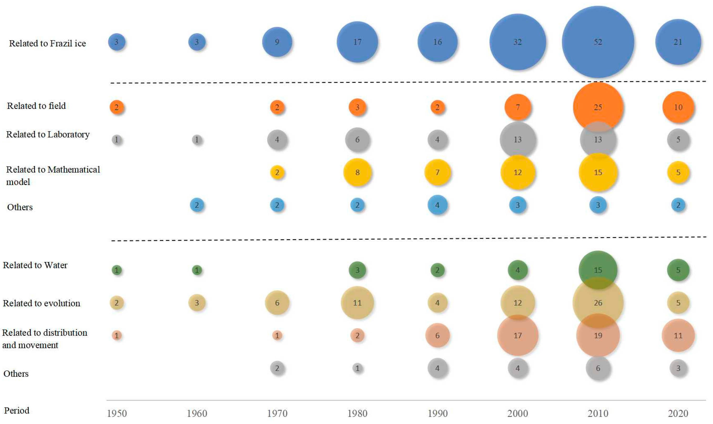
In order to quantify the progress of scholarly research on “frazil ice evolution”, a long time series of relevant articles was reviewed. Since this paper focuses on the evolution of frazil ice in freshwater rivers and channels, we searched the abstract and citation database Scopus with the string “frazil ice and evolution” and “not sea and not ocean” to identify 153 highly relevant papers; we present the chronological order of the publications in Figure 1. The papers counted include both journal papers and conference papers, and at least the originals or abstracts can be downloaded from the web, as some of the older papers are no longer available in their original form and the abstracts cannot be found online. The papers were further categorized according to the research methods and objects used by their authors. The research methods include field observations, laboratory experiments, numerical simulations, and others (reviews, theoretical analyses, and risk assessments of frazil ice damage), and the research objects include water temperature, frazil ice evolutionary processes, frazil ice motion and distribution, and others (e.g., an introduction to frazil ice observation techniques and devices, an overview of problems caused by frazil ice). Based on the number of papers counted, there were fewer studies on frazil ice before the 20th century. This may be because researchers believed that the evolution of frazil ice occurs during the initial stage of the ice development process and does not have a significant impact on river ice problems; on the other hand, it may be because the frazil ice is very small and its evolution is a microphysical process that is difficult to observe directly. Since the twentieth century, with the advancement of electronic technology, a variety of observation devices and techniques have been designed, and the number of frazil ice studies has increased significantly [7,8,9]. At the same time, the research methods were not only limited to laboratory experiments; field observations also increased. This shows that the evolution of frazil ice is gradually gaining attention from scholars and is an important part of the research on river ice.
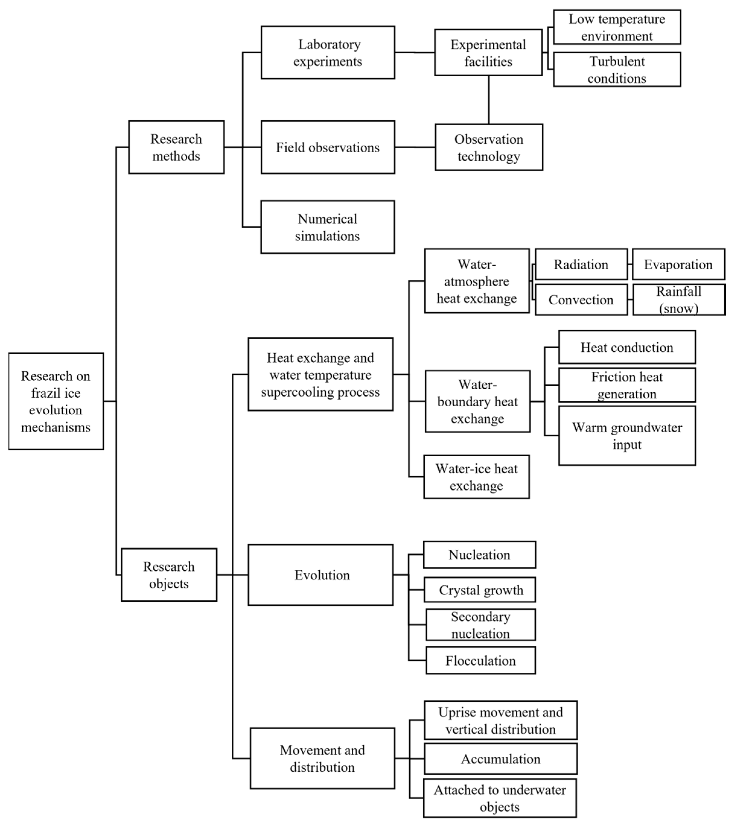
In this paper, we briefly introduce the techniques and methods used to observe the evolution from field measurements and laboratory experiments, and we summarize the observed evolution and properties of frazil ice, including nucleation, thermal growth, secondary nucleation, collisional fragmentation, and flocculation. We also focus on the numerical methods that are currently used to simulate the evolution of frazil ice and present the research on the movement and distribution of frazil ice (Figure 2). By summarizing and analyzing the existing research on frazil ice, we propose further research focuses and research directions, including the coupling of results from two observation techniques, deducing frazil ice variation from water temperature, the numerical simulation of the nucleation process, the mechanisms and simulation of the frazil ice collision process, and the three-dimensional simulation of frazil ice movement and distribution.
2. Laboratory Studies and Field Observation
When the evolution of frazil ice is not well known, the laboratory simulation of frazil ice is an effective way to learn more about its evolution mechanism and processes. In contrast to field observations, which are limited by the randomness of the natural conditions when collecting the data, researchers can easily control devices such as pumps or propellers in the laboratory to create precise water flow conditions, precisely control the ambient temperature through temperature systems in a confined space, and observe the evolution of the frazil ice in detail with the help of image acquisition and post-processing techniques [8]. Laboratory-scale physical model tests are primarily biased toward the study of the mechanisms of frazil ice’s evolution, so they can meet the test requirements without using an oversized water container. This section does not summarize the methods used to create a low-temperature environment in the experiments, because the researchers basically conducted the experiments in a confined, temperature-regulated space. Barrette [10] has provided a thorough review of the developments in laboratory research on the evolution of frazil ice, so this aspect is only briefly summarized in this article.
2.1. Laboratory Studies
2.1.1. Experimental Facilities
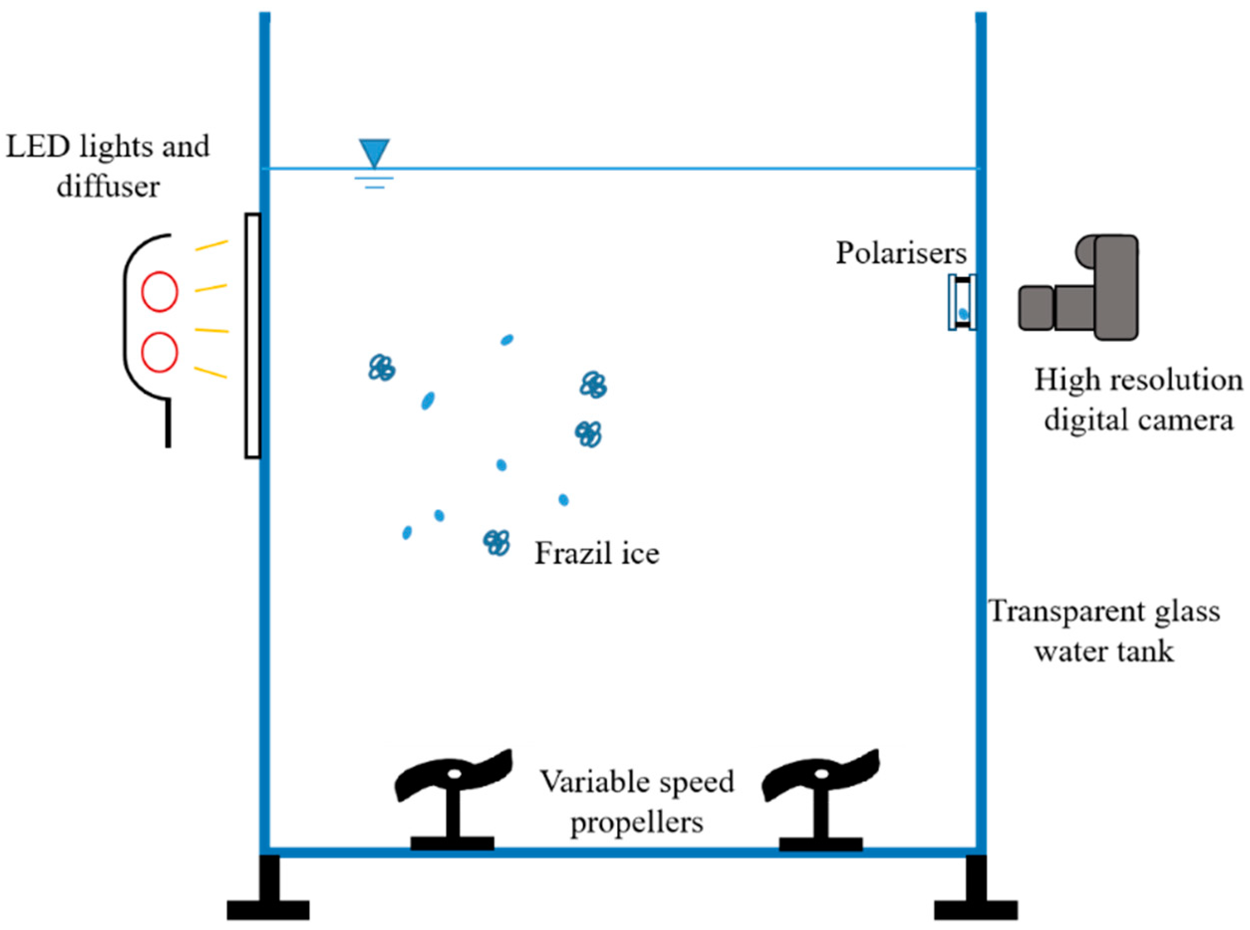
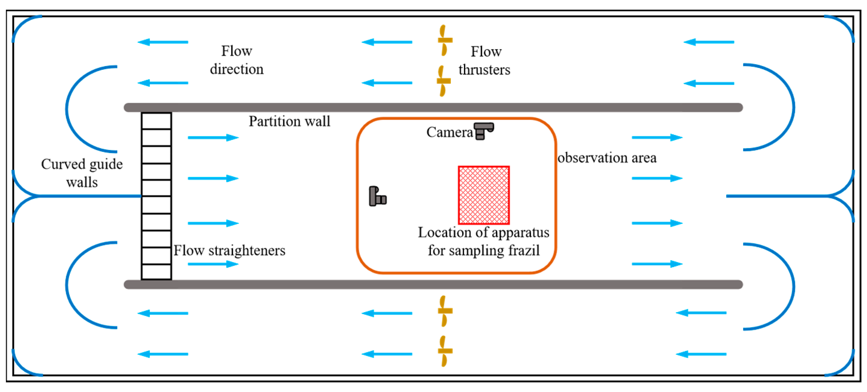
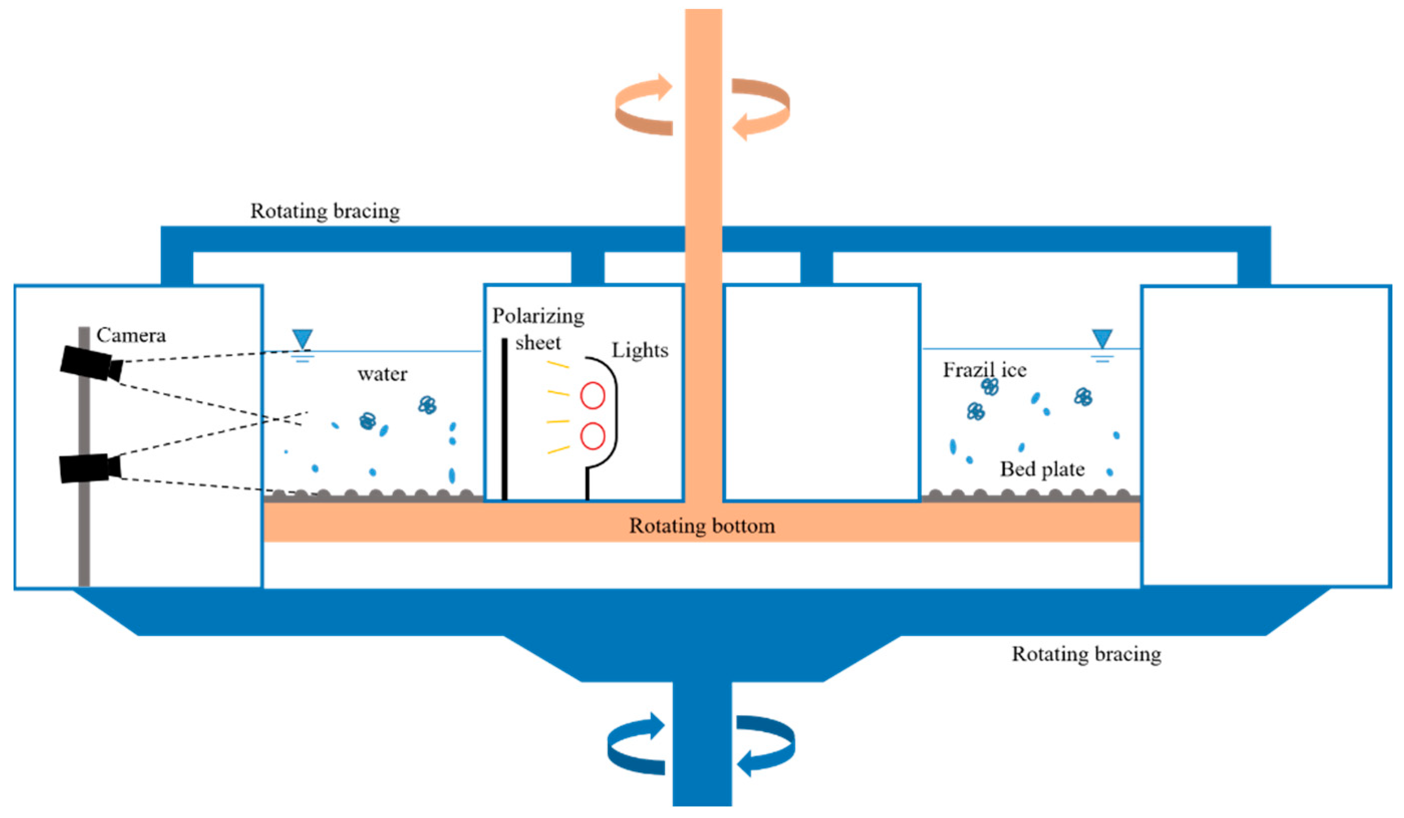
Many experimental studies on frazil ice have been carried out since the middle of the last century [11,12,13,14]. Michel [15] performed simulations of water supercooling processes and experiments on the evolution of frazil ice generation in an outdoor flume in 1963. Carstens et al. [16] used an indoor elliptical recirculating flume for frazil ice studies, where the water flow was generated by a variable-speed propeller and the water cooling rate was controlled by a fan blowing air set in the straight section of the flume. Hanley and Michel et al. [11,17] used a cold chamber to simulate low temperature conditions, where a controlled variable-speed propeller was installed in a cylindrical steel tank to drive the water flow. The turbulent flow conditions were generated by the flow of water around the central axis of the cylinder. Additionally, Tsang [18] used rectangular tanks, Ettema et al. [19] used turbulent tanks, McFarlane et al. [9,20,21,22] used square glass water tanks (Figure 3), and Richard [23] designed a new runway-type circulating water tank (Figure 4). Researchers have supplemented these water-holding devices with controlled water flow drives to create turbulent conditions that approximate those of a natural river. As seen from the above experimental facilities, the conditions required for researchers to simulate frazil ice evolution in laboratory experiments are relatively simple and easy to control. However, in these experiments, there are some thermal and mechanical factors that affect the accuracy of the results, such as the heat generated during the operation of the pump, which affects the water temperature, and the collision between the propeller blades and the frazil ice, which changes the particle size, etc. Therefore, it is necessary to avoid the influence of the experimental facilities on the evolutionary process as much as possible to ensure the accuracy of the experimental process. Clark et al. [24,25,26] designed a counter-rotating flume device (Figure 5), which creates turbulence by reversing the rotation of the flume’s bottom plate and the side walls. The intensity of the turbulence is adjusted by varying the roughness of the rotating bottom plate. This experimental approach prevents the heat generated by the pump and the mechanical action of the propeller from affecting the evolution of the frazil ice generation.
2.1.2. Observation Instruments
Although the conditions of frazil ice generation can be simulated, early in the history of frazil ice studies, there were few reliable observation methods, especially when the frazil ice particles are very small [27]. Schaefer [28] used a microscope to observe the morphology. Arakawa [29] designed the shadow photograph method and collected photos of frazil ice. With the progress of technology, different methods have been designed for the quantitative observation of frazil ice. For instance, Schmidt [30] used a commercial laser doppler velocimeter optical system, which works in conjunction with specially designed electronic circuits; meanwhile, an underwater frazil ice detector was developed by Tsang et al. [31], which uses the difference in water resistivity to estimate the frazil ice concentration. Daly et al. [32] developed a device that obtains the frazil ice concentration by measuring the flow through a filter and the frazil ice accumulated on the filter; Pegau et al. [33] used two kinds of optical instruments to obtain measurements of frazil ice concentrations, a method that was proven to be effective through experiments in the laboratory. Marko et al. [34,35,36] introduced the basic concept and working principle of SWIPS (shallow water ice profile sonar) for measuring river ice conditions and described the relationship between the data collected by the instrument and the characteristic parameters of ice conditions. By gathering the reflected signals from high- and low-frequency sonar on a specific body of water with a particular frazil ice concentration, Ghobrial et al. [37] investigated the use of underwater sonar technology for detecting frazil ice concentrations and established a regression equation between the intensity of the sonar backscattered signal and the frazil ice concentration. Richard [23] used acoustic sonar and underwater cameras to observe frazil ice simultaneously in an experiment and developed a bespoke frazil sampling frame, made by a rectangular piece of wire mesh, to rapidly collect samples of the frazil crystals. There are also other observation means, such as calorimetric devices [38].
In addition to the techniques mentioned above for observing frazil ice, with the advancement of image acquisition and post-processing techniques, the precise morphology and quantity of minute ice particles have gradually been observed, and the generation and evolution of frazil ice have become increasingly better understood. MacFarlane et al. [20,21] and Doering et al. [39] designed frazil ice image acquisition systems based on the same principle; these consist of a high-resolution digital camera, LED lights or light emitting diodes, and polarized filter glass sheets (Figure 3). The square polarizing filters are spaced at a certain distance from each other and installed in parallel on the side of the glass tank near the digital camera placement. The frazil ice that moves with the water flow to the middle of the polarizing filter is illuminated by the diodes and then captured by the digital camera. The image is further post-processed by analyzing the original image and using the Matlab algorithm to determine the threshold value, undertake image enhancement and weakening, and conduct binary image analysis and particle identification, among other procedures, to identify the ice particles in the image. Next, the characteristics of the ice distribution in the water throughout the course of the test are obtained, including changes in the quantity, size, concentration, and vertical distribution of the ice. MacFarlane et al. [9] demonstrated the effectiveness of this post-processing method by manually examining nearly 1000 ice particles in the images; they verified that the accuracy of this algorithm in correctly identifying ice particles in water was over 93%. According to the technical principle, the above observation methods can be divided into two types: signal (electrical, optical, and acoustic signals) measurement systems and image acquisition systems. In terms of application scenarios, the signal acquisition system can be applied to the measurement of frazil ice concentrations in regional waters, while the image acquisition system can accurately observe the shape, size, and quantity of frazil ice, but the observation range is small and only applicable within the camera’s shooting range. Both observation methods have been used in field observations.
2.2. Field Observation
Given the above analysis, it is clear that it is more convenient to observe the development of frazil ice generation in a laboratory setting than in a natural river or channel during the winter. However, artificially created low-temperature and turbulent conditions are different from those of a natural river or channel. Researchers have made an effort to observe the evolution of frazil ice in natural rivers, despite the challenging operating environment and observation methodologies that often limit field observations. Gilfilian et al. [40] observed the ice formation process in small streams in the Fairbanks area of the United States, and measured hydraulic parameters such as the amount of supercooling, the supercooling time, and the radiative heat balance on a diurnal scale. Richard et al. [41] used multi-frequency hydroacoustic instruments to observe frazil ice in the St. Lawrence River and introduced a frequency inversion method to estimate the characteristics and concentration of frazil ice. Ghobrial et al. [42] deployed underwater high- and low-frequency sonar to collect frazil ice acoustic data and discussed the use of scattering models to estimate frazil ice concentrations and particles sizes from acoustic signals; they investigated the applicability of three scattering models, as well as empirical regression equations, for the measurement of frazil ice concentrations. Marko [43,44], Dmitrenko [45], Ito [46,47,48,49], Eamon [50], and others similarly used sonar systems to observe the characteristics and distribution of frazil ice; although used in the observation of ocean frazil ice, these researches have similarly demonstrated the feasibility and effectiveness of sonar sounding in the field observation of frazil ice. The above measurement methods that use acoustics are used indirectly for frazil ice measurement, and naked-eye in situ measurements are not common. Osterkamp et al. [51] presented photographs of various forms of frazil ice in inland rivers; elsewhere, MacFarlane et al. [52,53] placed a laboratory-validated image acquisition system in three Alberta rivers and accurately measured the frazil ice in these rivers. The size, shape, size distribution, and volume concentration of frazil ice in the rivers were measured. The observations of the parameters were in general agreement with the laboratory results, except that the average particle size range was slightly smaller than in the laboratory observations due to snowfall at the time of the observations, and the prototype observations and physical model tests corroborated each other. It can be seen that signal measurement systems are mostly used to collect information on frazil ice concentrations in field observations, while the application scenarios for image acquisition systems are less common, probably because the range of water bodies that can be observed using image acquisition systems is small, and, even if the results can be applied inverted to regional waters, their accuracy may be reduced due to the complexity of natural water flow conditions.
As a result, it would appear that, while laboratory simulations of frazil ice tests have the benefits of being easier to perform and having controllable working conditions, they are unable to completely eliminate the issues associated with human interference and the lack of natural environmental conditions. Field observations, however, can avoid these issues but are constrained by the challenging nature of the observations and the demanding instrumentation needs [40]. Signal measurement systems and image acquisition systems are both currently the most widely used frazil ice observation methods. The two techniques differ in terms of the range of observations and in the results obtained for frazil ice, so each has its own focus when applied. The increasingly large observation range and more accurate observation results represent the future development direction of frazil ice observation in rivers and channels. Consequently, it would benefit frazil ice observation and monitoring in rivers and channels if a closer link were developed between data from signal measurement systems and the specific characteristics from image acquisition systems. In this way, the signal measurement system not only measures the frazil ice’s concentration but also deduces precise information such as the number and size of frazil ice particles.
3. Heat Exchange and Supercooling Processes
Water temperature measurement is a crucial component of field observations and model studies in the winter because it has a significant impact on the evolution of the river ice [54,55,56,57,58,59,60,61,62,63,64,65]. Researchers gather water temperature data during ice field observations and laboratory experiments using a significant quantity of high-accuracy temperature sensors to determine the water temperature change process and analyze the influencing factors as the basis of the analysis of the evolution of frazil ice.
3.1. Heat Exchange
The change in water temperature is influenced by the water–external heat exchange process and the water–ice heat exchange process, where the water–external heat exchange comprises water–atmosphere heat exchange and water–boundary heat exchange.
3.1.1. Water–Atmosphere Heat Exchange
The evaporative condensation heat flux, long-wave radiation, atmospheric short-wave radiation, and water–air convection heat transfer are all included in the category of water–atmosphere heat exchange. Shen et al. [7] provided a detailed description of each heat exchange process, as well as the calculation equation (Table 1, No. 1), when researching the river ice process. This calculation method can determine the flux in the water–atmosphere heat exchange more accurately, but it requires a large number of parameter values for solar radiation, the longitude and latitude of the river, rainfall or snowfall, cloud cover, wind velocity, saturated vapor pressure, etc. When the specific values of some parameters are difficult to obtain, the heat exchange flux can also be calculated using a linear approximation evaluation, i.e., the generalized linear method, when the basic data are not sufficient and the parameters cannot be accurately estimated (Table 1, No. 2). The value of hwa is assumed to be essentially the same everywhere at the same latitude for the selection of parameters in this method, and 20 W/(m2·°C) is typically taken as the value for rivers in the United States and at high latitudes in northern China [66]. The heat exchange coefficient hwa is derived from numerous observed experimental datasets and is not precise enough for short-term forecasting, despite the generalized linear algorithm being easy and quick to calculate. Hence, accurate calculations of the water–atmosphere heat flux that use processes such as atmospheric radiation and water–air convective heat transfer are still required when conditions permit it. Richard [67] also presents heat budget and heat transfer equations (Table 1, No. 3). Like Shen’s model, Richard’s heat transfer model also considers long-wave radiation, short-wave radiation, water–-air convection heat transfer, and evaporative condensation heat flux, but Richard also takes into account the effect of precipitation on the water temperature, and provides a formula for heat fluxes due to precipitation.
3.1.2. Water–Boundary Heat Exchange
The riverbed (channel) temperature relative to the water temperature induced by heat conduction, the generation of friction heat by the water and riverbed (channel), and the bottom of the riverbed’s warm groundwater input are all aspects of the water–boundary heat exchange process. However, the water and riverbed’s (channel) generation of friction heat and the bottom of the riverbed’s warm groundwater input are often neglected in numerical calculations, because the fluxes of these two heat exchange processes are extremely small compared to the other heat transfer fluxes, and it has no effect on the calculation results when these two processes are ignored. The thermal conductivity of the sediment, the vertical temperature gradient close to the riverbed (channel), and the water temperature are the key determinants of the conductive heat exchange between the water and the riverbed (channel). Due to the greater difficulty of measuring them, these variables can only be approximated [67]. Shen and Ruggles [68] calculated the heat transfer between the water and the riverbed to be roughly 8.5, 11, 8, 6, 4.5, and −2.2 W·m−2 on the beginning of every month between November and April. Evans et al. [58] calculated it to be about 5 W·m−2 in November. This indicates that the heat flux between the water and the boundary (river channels, etc.) is small and the heat exchange between water and external sources mainly comprises water–atmosphere exchanges [7,68].
3.1.3. Water–Ice Heat Exchange
The water–ice heat exchange consists of conduction and convection between the water and the frazil ice. The heat flow is calculated from the product of the temperature difference between the water and the ice and the heat exchange coefficient (Table 1, No. 4). The parameter to be noted in the heat transfer coefficient calculation is the Nusselt number (Table 1, Nos. 7,8). The Nusselt number represents the ratio between the actual (potentially turbulent) heat transfer rate and the heat transfer rate through conduction alone [69]. When ice particles are suspended in idealized, absolutely stationary water, i.e., Nu = 1, only conduction occurs. The amount of convective heat transfer between water and frazil ice is judged by the size of the ice particles and the smallest eddies present in the bulk flow [70]. If the particle size is smaller than the smallest existing eddies, Nu increases to a little above 1. When a crystal is larger than the existing eddies, the value of Nu will be considerably greater than 1. In the formula for calculating hwi, l represents the characteristic length of particles, but researchers have sometimes taken a different approach to the value. Daly [12] parametrized the Nu values of the large and small size particles based on experiments and theory, using the ratio of the ice particle radius to the minimum vortex scale, m*, as the criterion for judging the particles to be large or not (Table 1, No. 7). The parameter NuT reveals the relative heat transfer coefficient for each disc radius at a common length scale. The parameters Nu and NuT are easily confused [71,72,73] and need to be noted in the calculations. The current water–ice heat exchange model is well established and can be applied to all water–frazil ice heat exchange calculations with no limitations.

Table 1.
Heat exchange models involved in water temperature calculations.
| Model | No. | Year | Researcher | Formula | Remark |
|---|---|---|---|---|---|
| Heat transfer between water and air | 1 | 1984 | Shen [7] | is the heat transfer between water and air; is short-wave radiation, cal·cm−2·day−1 is the conductive heat transfer, cal·cm−2·day−1; is the incoming short-wave radiation, cal·cm−2·day−1; is the cloud cover in tenths; = 0.0017; c = 0.55; d = 0.052; , mb; is a coefficient, similar to the evapo-condensation flux; | |
| 2 | 1991 | Lai [74] | °C−1 °C; °C; | ||
| 3 | 2015 | Richard [67] | means the water experiences a heat loss or negative heat flux, and means the opposite; is the air temperature, °C; is the water albedo for long-wave radiation (approximately equal to 0.03); is the short-wave water surface albedo; is the air density; is the effective wind speed at a reference height; , , and , are the drag coefficients and heat transfer coefficients for sensible and latent heat, respectively is the specific heat of air; is the latent heat of vaporization (or sublimation); is the rate of falling snow mass per unit area; and are the temperature at the surface and the potential temperature (the temperature that a parcel of fluid would acquire if adiabatically brought to a standard reference pressure) at a reference height, respectively; are the humidity at the surface and the potential specific humidity at a reference height, respectively; | ||
| Heat transfer between water and frazil ice | 4 | 1984 | Omstedt [75] | is the coefficient of the heat exchange between water and ice; is the Nusselt number, is the radius of the spherical ice particles, i = 1, 2…. | |
| 5 | 1985 | Omstedt [76] | is the thickness of the ice crystal; | ||
| 6 | 1994 | Svensson [77] | |||
| 7 | 1984 | Daly [12] | For large particles, i.e., m* > 1: | ; is the “turbulent” Nusselt number; is the Prandtl Number; is the turbulence intensity; U is the mean flow velocity. | |
| 8 | 2007 | Holland [69] | A correction to “Frazil evolution in channels” by Lars Hammar and Hung-Tao Shen [70]. |
3.2. Supercooling Process
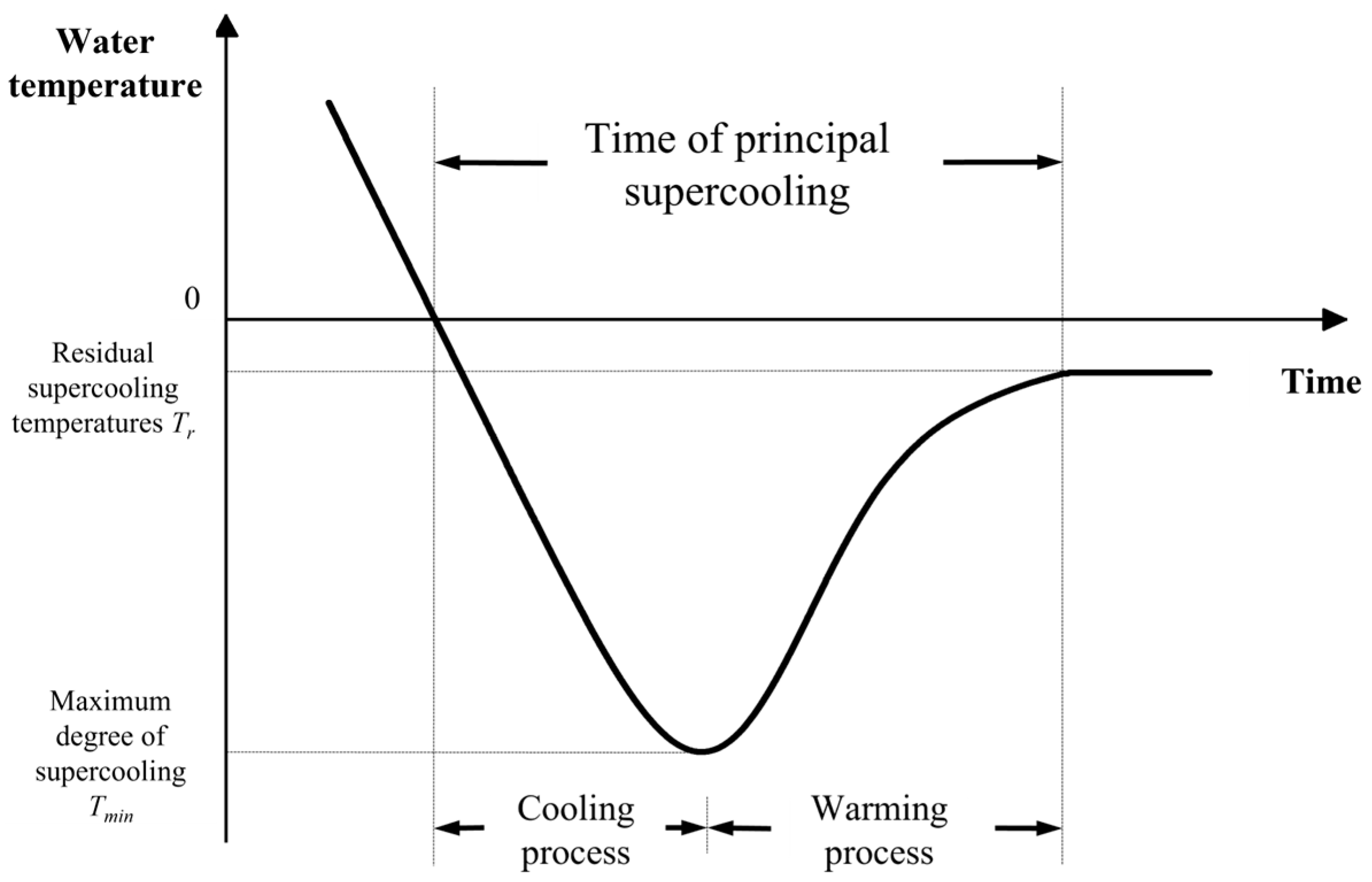
According to various studies [8,9,24], in a typical body of water during the evolution of ice formation, the water temperature displays a change curve similar to that shown in Figure 6. The entire change process is divided into the main supercooling phase and the residual supercooling phase, in which the main supercooling process exhibits a trend of first cooling and then warming when the formation of frazil ice accelerates. The entire change process is governed by the heat exchange of water. Water bodies and the atmosphere, river and canal boundaries, and other external heat exchanges that cause outward heat dissipation cause the water temperature to continue to decline over the winter, a process known as supercooling. The water body will enter a condition of supercooling and the production of frazil ice is initiated when the water temperature drops to 0 °C and continues to lose heat [24,78], and frazil forms faster when the rate of supercooling is greater [79]. As frazil ice forms and expands, latent heat is released into the water body around it, raising its temperature and reducing the amount of supercooling experienced by the water. The water temperature rises from the maximum supercooling temperature Tmin to a stable supercooling temperature Tr when the rate of the latent heat release from the ice in the water exceeds the rate of heat loss from the water body to the outside. According to laboratory research [8], there is a strong correlation between the water supercooling process and the external temperature and the depth of the water in the tank. A colder external temperature will result in a shorter supercooling process and a lower maximum supercooling degree, whereas a deeper external water layer will prolong the main supercooling process and reduce the maximum supercooling value. It has been demonstrated that the residual supercooling temperature Tr ranges from 0 °C to −0.01 °C and that the maximum supercooling degree Tmin of the supercooling process spans from −0.03 to −0.1 °C [8,9,24,25,80,81].
The water temperature variation outdoors is more complex than that in indoor experiments because of atmospheric temperature changes, the formation of ice cover that prevents heat exchange, shore obstacles that block heat radiation, and anthropogenic heat input (urban drainage, dam discharge, etc.), but it essentially maintains the variation pattern of supercooling, warming, and stabilization [82]. Boyd et al. [82,83] conducted a multi-year study of Canadian rivers and took multi-year measurements of winter water temperature changes in three rivers in Alberta. They found that the cooling rates in the rivers were, on average, approximately one order of magnitude lower than those in the laboratory. They attributed this difference to the indoor tests being carried out in tanks with shallow water depths and uninsulated sides and bottoms, resulting in a heat exchange between the water and the tank walls. As discussed in the previous section, the water temperature is determined by the heat exchange between the water and each element, which also includes the water–ice heat exchange process. Therefore, researchers have tried to determine the evolution of frazil ice generation according to the water temperature subcooling process. Boyd et al. fitted a linear relationship between the seasonal cumulative degree minutes of supercooling (SCDMS) and the freeze-up time based on measured data. In their observations of natural river ice, Howley et al. [84] introduced the degree minutes of supercooling (DMS), which was defined as the supercooling process, in response to the problem of the ice in the water blocking the water intake. The integrated area of the water temperature time series (i.e., the area of the region where the 0 °C and supercooling curves are closed) was also proposed to use DMS to quantify the intensity of the supercooling event and to relate it to the evolution of frazil ice production for the prediction of frazil ice quantities or concentrations by water temperature supercooling. This study is feasible because water temperatures are mainly determined by the water–atmosphere heat exchange and the water–ice heat exchange; if the water–atmosphere heat exchange can be calculated, then the water’s temperature change can predict the extent of the water–ice heat exchange, so as to determine the change in the frazil ice. At the same time, whether in the laboratory or in the field, the measurement of water temperatures is relatively simple and convenient, so this study can provide support for rapid ice analysis and predictions. To date, there are few related studies, but more can be conducted in the future.
4. Frazil Ice Generation and Evolution
In both lab and field studies, it has been discovered that the supercooling process, or the evolution of frazil ice production, causes changes in the size, shape, and quantity of frazil ice. According to the results of the current study, nucleation, growth, secondary nucleation, and flocculation are the primary stages in the evolution of frazil ice, and many mathematical models have been developed [71,73,76,77,85,86,87,88,89]. These processes are discussed below.
4.1. Nucleation
When the body of water is in a supercooled state, ice crystals begin to form; the temperature at which the water condenses into ice crystals mainly depends on the presence of foreign particles. In the absence of foreign bodies, and in still pure and impurity-free water, the water molecules may undergo random nucleation and thus large-scale condensation, also known as homogeneous nucleation. In the presence of foreign bodies, water molecules condense in the direction of the foreign body under the action of the interfacial force field; this is known as heterogeneous nucleation [90]. The water temperature for homogeneous nucleation must be below −40 °C, while the presence of foreign matter encourages an increase in the supercooling temperature during condensation. The nucleation and icing processes that occur in nature are all heterogeneous nucleation processes [3,91,92]. Academics currently believe that nucleation comes from impurities in water and crystals from the air (such as dust, snowflakes, droplets, or ice crystals in moist air) [12,93,94,95]. Doering et al. [8,25] used a reverse-rotating flume to observe the evolution of ice within the water. The flume was sealed during the experiment, and no outside ice species entered the water body, but ice crystals still formed. Since the water in the flume is tap water rather than pure water, the ice crystal nuclei in the experiment may have come from impurities in the water. In nature, when turbulence of the flow is low, the water column near the surface is subcooled faster than the lower layers and there is an input of crystals from the air, so the ice particles first form on the surface of the water column, and, when the turbulence intensity rises, the surface ice particles are carried by the turbulence into the interior of the water column as the nuclei of frazil ice. A different theory regarding the nucleation mechanism, however, has been advanced by some researchers; it has been discovered that the cavitation bubbles and water-soluble gas microbubbles created by turbulence can also start the process of frazil ice nucleation [96,97]. The triggering mechanism is connected to the local dissipation of turbulent energy [3], and these microbubbles can stay in the water for a longer period of time, which may also be the cause of the increasing amount of frazil ice. Additionally, a recent study demonstrated that the formation of ice crystals originates from the tiny bubbles created when supercooled water droplets land on the water’s surface [98].
The calculation of the initial nucleation of frazil ice is important because it is the initial condition for the beginning of the frazil ice evolution process. However, the initial numerical simulations of the nucleation process are currently simple. In numerical simulations, the current nucleation process is essentially sped up by supplying a predetermined number of ice crystal nuclei in the water column when the nucleation requirements are satisfied, either experimentally as a constant value of the initial conditions for beginning the ice evolution process [73,77], or as a linear function of the time dependence, i.e., a constant growth rate of the number of ice crystal nuclei [71]. This is because the current technology is unable to observe extremely small-scale ice nuclei and cannot visually monitor the formation and change process of ice nuclei. However, the accuracy of the simulation is constrained in different environments when using only the current numerical simulation methods, because the initial nucleation process (wind, blowing snow, snowfall, rainfall, or water flow conditions) varies significantly in different environments under natural conditions. Therefore, further research is needed to establish a numerical model for the initial nucleation process of frazil ice.
4.2. Crystal Growth
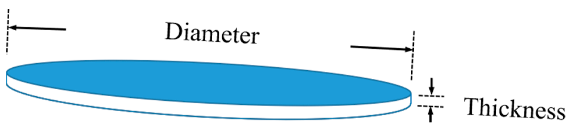
When ice nuclei form, they exchange heat with the supercooled water body and release heat, causing them to expand. It has been observed that frazil ice can have a variety of morphologies, including thin discs, dendritic structures, hexagonal stars, and irregular shapes [5] (Figure 7), depending on the heat transfer conditions between the ice crystals and the environment, as well as inter-crystal interactions [12,40]. Daly [27] detailed the causes of such shapes of frazil ice based on earlier research [99]. There is a parameter, α, that characterizes the roughness of the solid–liquid interface; when α > 2, the solid–liquid interface is smoother, whereas, when α < 2, it is rougher. According to Fujioka [100], the thickness direction’s value is 2.64, whereas the diameter direction’s value is 0.88. As a result, water ice grows more quickly in the diameter direction than in the thickness direction, finally taking on the shape of a thin disc. According to observations from laboratory studies, a frazil ice disc has a width–thickness ratio of around 1–100 (the ratio of the disc diameter D to the thickness t) [21,101,102,103,104,105].
Frazil ice grows at a rate determined by the rate of the heat exchange between it and the water column, which is regulated by the degree of water flow turbulence [71]. It has been demonstrated that the frazil ice particles in water are able to grow faster and may expand to greater crystal sizes as the turbulence severity increases. The latent heat released into the water by the ice crystals increases as the ice in the water grows, slowing the pace of cooling until the water temperature starts to rise after the supercooling temperature reaches a minimum and the development rate of the ice crystals starts to slow down. In mathematical models, the volume of ice crystal growth is often determined by dividing the latent heat of ice, which causes an increase in the size of the ice crystals, by the heat exchange flux between the ice and the water. Svensson et al. [77] proposed the ice volume change per unit time from crystal development at the i-th radius grouping for various size groups (Table 2, No. 1). Hammar [71] used the volume concentration to express the frazil ice variation for each particle size group (Table 2, No. 2).
4.3. Secondary Nucleation and Flocculation
According to observations of the evolution of frazil ice generation, the number of ice particles increases significantly at a certain point, gradually declines after reaching a peak, and then finally finds a stable condition. In response to this phenomenon, the academic community proposed that there is a mechanical effect in the evolution that causes the change in quantity. This process, known as secondary nucleation, occurs when the size of the frazil ice increases along with the ice–water heat exchange, or when large ice particles themselves cannot withstand the intensity of turbulence, leading to breakage. It can also occur when the turbulent movement of the ice particles in the water results in collisions between particles and, consequently, breakage. In addition to causing fragmentation when ice particles collide, collisions can also result in flocculation, i.e., the formation of centimeter-sized flocs due to the bonding of ice particles.
Turbulence intensity plays an important role in the secondary nucleation and flocculation processes [25,106]. Ettema [106] showed that turbulence intensity affects the secondary nucleation rate. Clark [25] found that the mean and standard deviation of particle size increased with the turbulent kinetic energy dissipation rate. According to Clark’s study, the mean and standard deviation of particle size rose as the turbulent kinetic energy dissipation rate rose, but they fell as the dissipation rate rose above 900 cm2/s3. The analysis reveals that an increase in the turbulence intensity causes an increase in the number of ice crystal collisions, which increases the size of the flocs, but there is also a higher turbulence intensity that overwhelms the strength of the ice particles and causes fragmentation, limiting the growth of the average floc size. This finding is also supported by the photos captured by Clark’s experiments: flocs created in high-turbulence-intensity water are denser in their early and late phases of growth and have a constrained final size. On the other hand, it has been found that condensates generated in water with low levels of turbulence intensity are initially sparser and more fragile, and as they grow larger and become more porous over time.
Mathematical models that simulate the secondary nucleation and flocculation processes have been proposed. Svensson and Omstedt [77] proposed the secondary nucleation model, which determines the number of secondary nucleations based on the number of frazil ice particles in the volume “swept” by the motion of a single particle per unit time; they also introduced an upper limit on the number of frazil ice particles per unit volume in this model to prevent the collision frequency from increasing after the concentration of frazil ice particles increases to a certain value (Table 3, No. 1). Hammar [71] simulated the secondary nucleation process and determined the number of nucleations that resulted from the collision of each size of particle with each other size, using a model created by Evans [107] (Table 3, No. 2). It is worth noting that the research presented in Evan’s article belongs to other disciplines, but the collisional secondary nucleation model developed is of great value for understanding the evolution of frazil ice (Table 3, No. 3). At the same time, the three models differ in terms of the calculation of the number of secondary nuclei after collisions. Svensson’s model assumes that only one nucleus is produced in a single interparticle collision, while the number of ice nuclei produced in Hammar’s model and Evans’ model is determined by the energy of the particle collision. In contrast, the calculation of the number of ice nuclei in Hammar’s model and Evans’ model seems to be more reasonable, but the calculation process is also more complicated.
In order to simulate the flocculation process within the model of ice collisional flocculation, the model used by Svensson and Omstedt [77] assumes a linear relationship and considers the fact that flocculation between larger ice particles is more likely to happen (Table 4, No. 1). Shen’s model [71] first determines the expected number of collisions per unit time for all particles in different size groups, and then reassigns the particles that change in size after collisional condensation to the group (Table 4, No. 2).
However, because the mechanism of the process has not been fully understood or replicated by researchers, the mathematical model used to represent the secondary nucleation and flocculation process has not advanced in recent years. Frazil ice collisions are dynamic motion processes, but the observation of ice particles is achieved by collecting independent and static images using a high-resolution camera at a specific frequency. The dynamic process can only be inferred and verified by static image results and changes in the quantity of ice and the particle size parameters, which is not sufficient. Therefore, the development of new observation techniques to observe the dynamic processes of frazil ice collisions and the development of new models for the secondary nucleation and flocculation of frazil ice are also topics for future research.
In summary, during the evolution of frazil ice, changes in the frazil ice grain size are subject to a combination of thermal growth, secondary nucleation, and flocculation, and have been observed to range in diameter from approximately 22 μm to 6 mm [3,9,24,27,106,108,109]; smaller ice crystals are not yet observable due to technical limitations [3]. Table 5 shows a summary of frazil particle sizes, measured optically or visually in some of the existing studies. In addition, McFarlane et al. [52] provide a detailed summary of the published data on frazil particle sizes. The number curve of each size distribution of frazil ice particles observed in the laboratory and in the field usually approximates the log-normal distribution [9,52,53,110].
5. Frazil Ice Movement and Distribution
Frazil ice is always entrained in the water flow when the buoyancy of the frazil ice particles is insufficient to overcome the vertical component of the water turbulence. The concentration of frazil ice rises as the water body continues to lose heat during the downstream transport phase. The higher the concentration of frazil ice, the greater the possibility of particles colliding with each other or contacting underwater objects. The particles either flocculate into larger particles up to the water’s surface, or become attached to the surface of objects such as rocks at the bottom of the riverbed, or become attached to and accumulate at the inlets of water intake facilities, resulting in a reduced overflow capacity, elevated water levels, and reduced diversion flow, as well as intake blockage and other problems.
5.1. Uprise Movement and Vertical Distribution
Since it is difficult to precisely estimate the rising velocity of frazil ice, little is known about the characteristics of surface frazil ice. Liou [111] presented a model for the evolution of frazil ice with time and depth in turbulent flows; the model relates the up motion of the frazil ice column to the influence of turbulent eddies. Ye et al. [112] created a numerical model for the vertical distribution of frazil ice and validated it utilizing the observed data obtained from laboratory experiments. Morse et al. [109] analyzed the evolution of frazil ice production in natural rivers using in situ data from the St. Lawrence River and analyzed parameters such as concentration gradients, size distributions, and the rise rate of frazil ice. Clark [81] employed image data to investigate the vertical distribution of ice particles inside the water column in a reverse-rotation flume experiment, paying particular attention to the impact of the turbulence strength. The findings indicated that the dispersion of ice particles inside the water column in the vertical range was more uniform the higher the turbulence intensity. Wang [113] developed a three-dimensional model to simulate the floating rates of frazil particles under an ice cover based on the theory of two-phase flow and laboratory data. The results indicate that the floating rates of ice particles are higher along the convex bank than along the concave bank at each cross section in the mathematical model, but the variation in the floating rate is relatively small for the prototype curved channel in large-scale models. Subsequently, the model is further optimized, so as to consider the influence of the liquid–solid interaction, which includes the interphase drag force, the lift force, the virtual mass force, the buoyancy force, and the volume fraction of ice [114]. MacFalane et al. [20] used an image processing algorithm to identify each particle and determine its diameter in a turbulent glass water tank. They then tracked the movement of each particle’s center of mass through a series of images to calculate the uplift velocity based on the total vertical displacement. The experimental process and the image processing algorithm are thoroughly described, and a novel function that connects the rising velocity to the diameter of the vertically rising disc is derived by comparing the measured data with the theoretical solution for the horizontal disc increase. However, the novel function does not consider the turbulent intensity of the water flow, because the rising velocities measured for two turbulence intensity conditions were found to be statistically similar to each other.
5.2. Frazil Ice Accumulation
When frazil ice moves downstream with the water flow, it accumulates when the water flow state changes (e.g., a rapid flow to a slow flow) or the water flow passes through a complex section (a bend, gate, or inverted siphon inlet). If the supply of frazil ice from the upstream reach continues, it will grow into a frazil ice jam, decreasing the flow area and posing hidden risks to the river’s safe operations [115]. Several studies have considered frazil ice processes in the near-surface layer. Shen et al. [116] looked into the evolution of frazil ice as an ice plug beneath the ice cover, proposed the concept of frazil ice transport capacity by analogy with sediment transport, and examined the effect of particle shape on transport capacity for the various shapes of frazil ice particles that may form in different rivers. Sui [117] discussed the role of transverse currents on frazil ice accumulation along a river bend and the characteristics of frazil ice accumulation. Ettema [118] studied the evolution and movement of frazil ice during pressure changes, focusing on the problems associated with frazil ice in pressurized conduits (pump-lines, penstocks, siphons, and tunnels) in mountainous regions, including the risk of frazil-related blockages in the conduits and blockage problems in downstream sections due to massive frazil ice generation at the outlet of the conduits. Fu et al. [119] conducted a real ice laboratory experiment for the accumulation and evolution of frazil ice in an inverted siphon inlet in a water conveyance flume. Although the size of the flow ice used in the test was not disclosed, the test images revealed that the ice accumulation was created by the agglomeration of frazil ice. Murray [120] investigated the flow characteristics under a freely floating jam made from discrete model ice pieces in the laboratory. The ice jam was formed by the accumulation of elliptical simulated particles with a major axis size of 5 mm, which allowed the flow to pass underneath the jam and through it. By using a PIV system to measure the seepage flow, bulk flow, etc., the movement process of frazil ice accumulation and scour can be analyzed more clearly. Chen [121] used 3.5 mm oblate elliptical simulated ice particles with a porosity of about 0.4 to study how hydraulic conditions and incoming ice discharge affect the formation of frazil ice jams through laboratory experiments; through a series of experiments, four different ice jam accumulation modes were detected.
Researchers have discovered that the accumulation and scouring processes of frazil ice under the action of water flow at the bottom of the ice cover is similar to the movement of riverbed sediments. Sui [122] carried out a series of experiments on the incipient motion of frazil particles under ice covers. Like the incipient motion of sediment particles on riverbeds, the relation between the shear Reynolds number and dimensionless shear stress for the incipient motion of frazil particles under ice cover have been established. It was found that, the steeper the ice cover slope, the higher the critical shear stress for the incipient motion of frazil particles; the opposite is the case for the motion of riverbed sediments. The critical shear stress required for the incipient motion of frazil particles is inversely proportional to the roughness conditions and proportional to particle size. Like riverbed sediment, ice accumulation waves refer to the downstream movement of frazil ice accumulation under the ice cover in the form of “waves” under specific flow and incoming ice conditions. Wang [123] revealed the mechanisms of ice accumulation wave formation and evolution through laboratory studies and investigated the conditions for wave formation and wave propagation velocity. The transport capacity of frazil ice under wave accumulation conditions was modeled by comparing the experimental results collected in the laboratory. Chen [124] established characteristic curves to determine whether ice waves occur under ice cover and analyzed the relationship between the ice wave migration speed and the ratio of the ice discharge to the water flow rate (Qi/Q). Hou et al. [125] studied the effect of bridge piers on ice wave migration, derived empirical equations to predict the thickness of ice waves, and investigated the thickness of wave crests and the migration rate of ice waves.
5.3. Attachment to Underwater Objects
In addition to its upward movement, frazil ice also moves with the entrainment of water and then becomes attached to submerged objects in supercooled conditions. Specifically, frazil ice can become attached to gravel in the riverbed and accumulate and grow, thus forming anchor ice. Anchor ice is of interest to researchers because it reduces the overflow cross section and restricts the flow, which raises the local water level as well as the water level upstream [126,127]. Early researchers observed the process of anchor ice formation through major in situ observations [28,126,127,128,129,130] and, subsequently, further investigated the factors that influence anchor ice development. Shen [131] and Hammar [132] determined that the formation of anchor ice is influenced by the frazil concentration, vertical mixing, the frazil size distribution, and the geometry and distribution of bed roughness. Through field observations, Hirayama [130] found that the development of anchor ice was related to the water flow Froude number. Doering [133] showed a relatively well-defined relationship between the rate of anchor ice growth and the Froude number by conducting a series of laboratory experiments performed in a counter-rotating flume. Kerr [134] designed a flume experiment for anchor ice generation and found that, during the initial stage of anchor ice growth, the anchor ice growth pattern depends on the flow rate and the Fr number. During the final stage, when the bottom of the flume is covered with ice, the growth rate is directly proportional to the heat loss rate and Fr number and is inversely proportional to the flow depth. Qu [135] also observed the effect of the Froude number on the forms of anchor ice and the effect of the extent of gravel roughness on anchor ice release by conducting a counter-rotating flume test. Bisaillon [136] recorded the meteorological and hydraulic conditions for anchor ice formation in three rivers in southern Québec (Canada) through field observations, developed a logistic regression model to predict the presence of anchor ice, and analyzed the effect of each explanatory variable (environmental and hydraulic conditions) on anchor ice formation, showing that the Fr number had the greatest effect on anchor ice. Stickler [137] studied the formation of anchor ice in natural rivers with different physical characteristics and classified anchor ice into two types by analyzing the growth and density of anchor ice: type I has a lower density and forms on top of the substrata, and type II has a higher density and forms between the substrata, filling interstitial spaces. The use of the water depth, flow velocity and boundary values of dimensionless numbers (the Froude number and the Reynolds number) to predict the spatial distribution of anchor ice was also investigated. Dube [138] collected underwater photographs of anchor ice and information related to the water level, water temperature, and air temperature in the field to understand the development process by studying the crystal type and size, the growth mechanism, the pattern and orientation, and the porosity of anchor ice accumulations. Ghobrial [139] designed an imaging system to acquire digital images of anchor ice formation and release on the riverbed and observed different mechanisms of anchor ice initiation, growth, and release. Meanwhile, in the field observations and laboratory experimental studies mentioned above, researchers have focused on the relationship between frazil ice and anchor ice development, and the results indicate that the attachment and accumulation effects of frazil ice promote the formation and growth of anchor ice.
In the research on the movement of frazil ice, another problem that troubles engineers and is related to actual production and human life relates to frazil ice blockages at the water intake. For this reason, researchers have carried out a great deal of work and put forward targeted solutions for specific situations [140]. Daly [141] presents an overview of frazil ice blockages of intake trash racks and describes the frazil ice blockage process, techniques (both those that are successful and those that are less so) for coping with frazil blockage, and guidelines for operating under frazil ice conditions. Chen et al. [142] used laboratory experiments and numerical simulation methods to study how the intake shape and size influence the intake ingestion of frazil ice; from the perspective of changing the water intake structure, they proposed ways to reduce ice intake in water. Daly [143] described a few case studies of blockages at intakes in the Great Lakes and provided useful insights into how blockages develop, as well as how their development could be relieved. Richard [144] studied how water intakes are vulnerable to frazil ice blockages and presented the environmental, temporal, hydraulic, and temperature conditions associated with these events according to field observations. Wang et al. [145,146] used Fluent software and a UDF module to simulate the three-dimensional water flow and ice movement in front of the water intake for the problem of drift ice blockages; a particle size of seven millimeters was used in Case 1, which has significance for the simulation of frazil ice at the three-dimensional scale. Kempema et al. [147] observed the whole process of the blockage of the wedge-wire screen at the water intake. The observations showed that the frazil ice particles or flocs were first attached to the screen, and then the water intake continued to be blocked by the growth of frazil ice and in situ ice growth, due, in part, to the increase in the relative water velocity once it was attached to the screen.
Based on the development of research on the motion and distribution of frazil ice, vertical rise, as the main motion component of frazil ice, has received more attention from researchers. Studies consider the vertical distribution, the uprise rate, and the influence of turbulence. Accumulation near the water surface is the final result of the uprising movement of frazil ice, but researchers seem to focus on the stage of process observation, characterization, and qualitative analysis of the accretion, and there is a lack of quantitative simulation studies. Based on the analysis, this may be because the forces acting on frazil ice in the accumulation body (drag force at the bottom or inside the accumulation body, buoyancy, etc.) are complex, and it is difficult to calculate the change in volume, the submergence depth, and other indicators of the accumulation body. The same is true for studies related to the attachment of frazil ice to submerged objects, which mostly focus on process descriptions and analyses of influencing factors. As a result, there is still a lack of knowledge on the mechanisms underlying the movement of frazil ice, as well as aggregation (deposition and flocculation), and there are few numerical simulations in this area, especially three-dimensional simulations. Currently, one-dimensional and two-dimensional models are being used by researchers to simulate the development of winter ice conditions because the longitudinal length of rivers and channels is significantly greater than the horizontal width. However, at some complex cross sections (bends, gates, or inverted siphon inlets) in rivers and channels, the water flow conditions are complex, and frazil ice tends to accumulate at these sections; thus, ice jams occur. At this point, a three-dimensional frazil ice movement and distribution model is particularly important because one-dimensional and two-dimensional models cannot simulate frazil ice’s movement and ice development in these sections. A three-dimensional model can derive the critical conditions for the occurrence of ice jams and blockages at these sections, so as to propose safe operation measures to reduce the risk of ice damage. Therefore, the establishment of a three-dimensional frazil ice movement and distribution model also deserves in-depth study in the future.
6. Conclusions
Icy conditions in rivers and channels in winter constitute a major problem for river catastrophe prevention and safe channel operations; they have a direct impact on typical human production, human life, and the ecological environment. The frazil ice evolution process has attracted a lot of attention because it is the first step in and the basis for the development of icy conditions in rivers and channels. Researchers have studied the nucleation, growth, collision, secondary nucleation, and flocculation processes of frazil ice through field observations, laboratory experiments, and numerical simulations, and the microphysical process of frazil ice evolution has become increasingly well understood as a result of the continuous advancement of observation technology. The authors of this review, however, think that the current study raises a few concerns that merit further attention and investigation:
- (1)
- The need for more applications of signal acquisition systems and image acquisition systems in field observations, and a close link between data from signal measurement systems and specific characteristics from image acquisition technology.
- (2)
- The need for a rational approach to determining the evolution of frazil ice generation by the water temperature subcooling process.
- (3)
- The need for numerical models for the initial nucleation process of frazil ice.
- (4)
- The need for new observation techniques to observe the dynamic processes of frazil ice collisions; then, more studies and new models on the secondary nucleation and flocculation of frazil ice.
- (5)
- The need for more studies on frazil ice movement and distribution and new three-dimensional frazil ice movement and distribution models for simulating frazil ice at complex cross sections of rivers and channels.
Future research on frazil ice will not be limited to the above areas, but, in any case, the evolution of frazil ice as the initial form of icy conditions should not be ignored. It is believed that future research can improve the frazil ice model and provide support for ice prediction and safety control in rivers and channels.
Author Contributions
Writing—original draft preparation, Y.C.; funding acquisition, J.L.; writing—review and editing, X.Z.; supervision, Q.G.; investigation, D.Y. All authors have read and agreed to the published version of the manuscript.
Funding
The authors are grateful for financial support provided by the Program of the National Natural Science Foundation of China with grant numbers U20A20316 and 51909186.
Data Availability Statement
The data presented in this study are available on request from the corresponding author.
Acknowledgments
The authors would like to thank the reviewers and editors whose critical comments helped in the preparation of this article.
Conflicts of Interest
The authors declare no conflict of interest.
References
- Hicks, F. An overview of river ice problems: CRIPE07 guest editorial. Cold Reg. Sci. Technol. 2009, 55, 175–185. [Google Scholar] [CrossRef]
- Beltaos, S.; Prowse, T.D.; Carter, T. Ice regime of the lower Peace River and ice-jam flooding of the Peace-Athabasca Delta. Hydrol. Process. 2006, 20, 4009–4029. [Google Scholar] [CrossRef]
- Makkonen, L.; Tikanmaki, M. Modelling frazil and anchor ice on submerged objects. Cold Reg. Sci. Technol. 2018, 151, 64–74. [Google Scholar] [CrossRef]
- Ashton, G.D. Frazil Ice, 49th ed.; Academic Press: Madison, WI, USA, 1983; pp. 271–289. [Google Scholar] [CrossRef]
- Schneck, C.C.; Ghobrial, T.R.; Loewen, M.R. Laboratory study of the properties of frazil ice particles and flocs in water of different salinities. Cryosphere 2019, 13, 2751–2769. [Google Scholar] [CrossRef] [Green Version]
- Zhang, Y.; Li, Z.; Xiu, Y.; Li, C.; Zhang, B.; Deng, Y. Microstructural characteristics of frazil particles and the physical properties of frazil ice in the yellow river, China. Crystals 2021, 11, 617. [Google Scholar] [CrossRef]
- Shen, H.T.; Chiang, L.A. Simulation of growth and decay of river ice cover. J. Hydraul. Eng. 1984, 110, 958–971. [Google Scholar] [CrossRef]
- Ye, S.Q.; Doering, J.; Shen, H.T. A laboratory study of frazil evolution in a counter-rotating flume. Can. J. Civ. Eng. 2004, 31, 899–914. [Google Scholar] [CrossRef]
- Mcfarlane, V.; Loewen, M.; Hicks, F. Measurements of the evolution of frazil ice particle size distributions. Cold Reg. Sci. Technol. 2015, 120, 45–55. [Google Scholar] [CrossRef]
- Barrette, P.D. Understanding frazil ice: The contribution of laboratory studies. Cold Reg. Sci. Technol. 2021, 189, 103334. [Google Scholar] [CrossRef]
- Hanley, T.; Michel, B. Laboratory formation of border ice and frazil slush. Can. J. Civ. Eng. 1977, 4, 153–160. [Google Scholar] [CrossRef]
- Daly, S.F. Frazil Ice Dynamics; US Army Cold Regions Research and Engineering Laboratory: Hanover, NH, USA, 1984.
- Daly, S.F.; Colbeck, S.C. Frazil ice measurements in Crrel’s flume facility. In Proceedings of the IAHR Symposium on Ice, Iowa City, IA, USA, 7–31 August 1986; pp. 427–438. [Google Scholar]
- Andres, D.D. Nucleation and frazil production during the supercooling period. In Proceedings of the Workshop on Hydraulics of Ice-Covered Rivers, Edmonton, AB, Canada, 1–2 June 1982; pp. 148–175. [Google Scholar]
- Michel, B. Theory of formation and deposit of frazil ice. In Proceedings of the 20th Annual Eastern Snow Conference, Quebec City, QC, Canada, 14–15 February 1963; pp. 130–148. [Google Scholar]
- Carstens, T. Experiments with supercooling and ice formation in flowing water. Geofys. Publ. 1966, 26, 1–18. [Google Scholar]
- Hanley, T.O.D.; Michel, B. Temperature patterns during the formation of border ice and frazil in a laboratory tank. In Proceedings of the 3rd International Symposium on Ice Problems, Hanover, NH, USA, 18–21 August 1975; pp. 211–220. [Google Scholar]
- Tsang, G.; Hanley, T.O. Frazil Formation in Water of Different Salinities and Supercoolings. J. Glaciol. 1985, 31, 74–85. [Google Scholar] [CrossRef] [Green Version]
- Ettema, R.; Karim, M.F.; Kennedy, J.F. A Study of Frazil Ice Formation; Army Cold Regions Research and Engineering Laboratory (CRREL): Hanover, NH, USA, 1984. [CrossRef]
- Mcfarlane, V.; Loewen, M.; Hicks, F. Laboratory measurements of the rise velocity of frazil ice particles. Cold Reg. Sci. Technol. 2014, 106, 120–130. [Google Scholar] [CrossRef]
- Mcfarlane, V.J. Laboratory Studies of Suspended Frazil Ice Particles; University of Alberta: Edmonton, AB, Canada, 2014. [Google Scholar]
- Mcfarlane, V.; Loewen, M.; Hicks, F. Field measurements of suspended frazil ice. Part I: A support vector machine learning algorithm to identify frazil ice particles. Cold Reg. Sci. Technol. 2019, 165, 102812. [Google Scholar] [CrossRef]
- Richard, M.; Cornett, A. NRC Frazil Ice Research Facility. In Proceedings of the Annual Conference—Canadian Society for Civil Engineering, Laval, QC, Canada, 2–5 June 2019. [Google Scholar]
- Clark, S.; Doering, J. Laboratory Experiments on Frazil-Size Characteristics in a Counterrotating Flume. J. Hydraul. Eng. 2006, 132, 94–101. [Google Scholar] [CrossRef]
- Clark, S.; Doering, J. Experimental investigation of the effects of turbulence intensity on frazil ice characteristics. Can. J. Civ. Eng. 2008, 35, 67–79. [Google Scholar] [CrossRef]
- Ye, S. A Physical and Mathematical Study of the Supe Rcooling Process and Frazil Evolution; University of Manitoba: Winnipeg, MB, Canada, 2002. [Google Scholar]
- Daly, S.F. Report on Frail Ice; International Association for Hydraulics Research, Working Group on Thermal Regimes: Madrid, Spain, 1994. [Google Scholar]
- Schaefer, V.J. The formation of frazil and anchor ice in cold water. Eos Trans. Am. Geophys. Union 1950, 31, 885–893. [Google Scholar] [CrossRef]
- Arakawa, K.; Higuchi, K. Studies on the Freezing of Water (I). J. Fac. Sci. Hokkaido Univ. II 1952, 4, 201–209. [Google Scholar]
- Schmidt, C.C.; Glover, J.R. A frazil ice concentration measuring system using a laser doppler velocimeter. J. Hydraul. Res. 1975, 13, 299–314. [Google Scholar] [CrossRef]
- Tsang, G. An instrument for measuring frazil concentration. Cold Reg. Sci. Technol. 1985, 10, 235–249. [Google Scholar] [CrossRef]
- Daly, S.F.; Rand, J.H. Development of an underwater frazil-ice detector. Cold Reg. Sci. Technol. 1990, 18, 77–82. [Google Scholar] [CrossRef]
- Pegau, W.S.; Paulson, C.A.; Zaneveld, J.R.V. Optical measurements of frazil concentration. Cold Reg. Sci. Technol. 1996, 24, 341–353. [Google Scholar] [CrossRef]
- Marko, J.R.; Jasek, M. Sonar detection and measurements of ice in a freezing river I: Methods and data characteristics. Cold Reg. Sci. Technol. 2010, 63, 121–134. [Google Scholar] [CrossRef]
- Marko, J.R.; Jasek, M. Sonar detection and measurement of ice in a freezing river II: Observations and results on frazil ice. Cold Reg. Sci. Technol. 2010, 63, 135–153. [Google Scholar] [CrossRef]
- Marko, J.R.; Topham, D.R. Laboratory measurements of acoustic backscattering from polystyrene pseudo-ice particles as a basis for quantitative characterization of frazil ice. Cold Reg. Sci. Technol. 2015, 112, 66–86. [Google Scholar] [CrossRef]
- Ghobrial, T.R.; Loewen, M.R.; Hicks, F. Laboratory calibration of upward looking sonars for measuring suspended frazil ice concentration. Cold Reg. Sci. Technol. 2012, 70, 19–31. [Google Scholar] [CrossRef]
- Lever, J.H.; Daly, S.F.; Rand, J.H.; Furey, D. A frazil concentration meter. In Proceedings of the International Association for Hydraulic Research Symposium on Ice, Banff, Alberta, 15–19 June 1992; pp. 1362–1376. [Google Scholar]
- Doering, J.C.; Morris, M.P. A digital image processing system to characterize frazil ice. Can. J. Civ. Eng. 2003, 30, 1–10. [Google Scholar] [CrossRef]
- Gilfilian, R.; Kline, W.; Osterkamp, T.; Benson, C. Ice formation in a small Alaskan stream. In Proceedings of the Symposia on the Role of Snow and Ice in Hydrology: Properties and Processes, Banff, AB, Canada, 6–20 September 1972; pp. 505–512. [Google Scholar]
- Richard, M.; Morse, B.; Daly, S.F.; Emond, J. Quantifying suspended frazil ice using multi-frequency underwater acoustic devices. River Res. Appl. 2011, 27, 1106–1117. [Google Scholar] [CrossRef]
- Ghobrial, T.R.; Loewen, M.R.; Hicks, F.E. Characterizing suspended frazil ice in rivers using upward looking sonars. Cold Reg. Sci. Technol. 2013, 86, 113–126. [Google Scholar] [CrossRef]
- Marko, J.R.; Jasek, M. Acoustic Detection and Study of Frazil Ice in a Freezing River during the 2004–2005 and 2005–2006 Winters. In Proceedings of the 19th IAHR International Symposium on Ice, Vancouver, BC, Canada, 6–11 July 2008; pp. 1–13. [Google Scholar]
- Marko, J.R.; Jasek, M. Multifrequency analyses of 2011–2012 Peace River SWIPS frazil backscattering data. Cold Reg. Sci. Technol. 2015, 110, 102–119. [Google Scholar] [CrossRef]
- Dmitrenko, I.A.; Wegner, C.; Kassens, H.; Kirillov, S.A.; Krumpen, T.; Heinemann, G.; Helbig, A.; Schröder, D.; Hölemann, J.A.; Klagge, T.; et al. Observations of supercooling and frazil ice formation in the Laptev Sea coastal polynya. J. Geophys. Res. Ocean. 2010, 115, C05015. [Google Scholar] [CrossRef] [Green Version]
- Ito, M.; Ohshima, K.I.; Fukamachi, Y.; Simizu, D.; Iwamoto, K.; Matsumura, Y.; Mahoney, A.R.; Eicken, H. Observations of supercooled water and frazil ice formation in an Arctic coastal polynya from moorings and satellite imagery. Ann. Glaciol. 2015, 56, 307–314. [Google Scholar] [CrossRef] [Green Version]
- Ito, M.; Ohshima, K.I.; Fukamachi, Y.; Mizuta, G.; Kusumoto, Y.; Nishioka, J. Observations of frazil ice formation and upward sediment transport in the Sea of Okhotsk: A possible mechanism of iron supply to sea ice. J. Geophys. Res. Ocean. 2017, 122, 788–802. [Google Scholar] [CrossRef]
- Ito, M.; Fukamachi, Y.; Ohshima, K.I.; Shirasawa, K. Observational evidence of supercooling and frazil ice formation throughout the water column in a coastal polynya in the Sea of Okhotsk. Cont. Shelf Res. 2020, 196, 104072. [Google Scholar] [CrossRef]
- Ito, M.; Ohshima, K.I.; Fukamachi, Y.; Mizuta, G.; Kusumoto, Y.; Kikuchi, T. Underwater frazil ice and its suspension depth detected from ADCP backscatter data around sea ice edge in the Sea of Okhotsk. Cold Reg. Sci. Technol. 2021, 192, 103382. [Google Scholar] [CrossRef]
- Frazer, E.K.; Langhorne, P.J.; Leonard, G.H.; Robinson, N.J.; Schumayer, D. Observations of the Size Distribution of Frazil Ice in an Ice Shelf Water Plume. Geophys. Res. Lett. 2020, 47, e2020GL090498. [Google Scholar] [CrossRef]
- Osterkamp, T.E.; Gosink, J.P. Frazil ice formation and ice cover development in interior Alaska streams. Cold Reg. Sci. Technol. 1983, 8, 43–56. [Google Scholar] [CrossRef]
- Mcfarlane, V.; Loewen, M.; Hicks, F. Measurements of the size distribution of frazil ice particles in three Alberta rivers. Cold Reg. Sci. Technol. 2017, 142, 100–117. [Google Scholar] [CrossRef]
- Mcfarlane, V.; Loewen, M.; Hicks, F. Field measurements of suspended frazil ice. Part II: Observations and analyses of frazil ice properties during the principal and residual supercooling phases. Cold Reg. Sci. Technol. 2019, 165, 102796. [Google Scholar] [CrossRef]
- Turcotte, B.; Morse, B.; Anctil, F. Cryologic continuum of a steep watershed. Hydrol. Process. 2014, 28, 809–822. [Google Scholar] [CrossRef]
- Turcotte, B.; Morse, B.; Anctil, F. Impacts of precipitation on the cryologic regime of stream channels. Hydrol. Process. 2012, 26, 2653–2662. [Google Scholar] [CrossRef]
- Cook, S.J.; Waller, R.I.; Knight, P.G. Glaciohydraulic supercooling: The process and its significance. Prog. Phys. Geogr. 2006, 30, 577–588. [Google Scholar] [CrossRef]
- Caissie, D.; El-Jabi, N.; Satish, M. Modeling of Maximum Daily Water Temperatures in a Small Stream Using Air Temperatures. J. Hydrol. 2001, 251, 14–28. [Google Scholar] [CrossRef]
- Evans, E.C.; Mcgregor, G.R.; Petts, G.E. River energy budgets with special reference to river bed processes. Hydrol. Process. 1998, 12, 575–595. [Google Scholar] [CrossRef]
- Turcotte, B.; Morse, B.; Anctil, F. The hydro-cryologic continuum of a steep watershed at freezeup. J. Hydrol. 2014, 508, 397–409. [Google Scholar] [CrossRef]
- Maheu, A.; St-Hilaire, A.; Caissie, D.; El-Jabi, N. Understanding the Thermal Regime of Rivers Influenced by Small and Medium Size Dams in Eastern Canada. River Res. Appl. 2016, 32, 2032–2044. [Google Scholar] [CrossRef]
- Lind, L.; Alfredsen, K.; Kuglerová, L.; Nilsson, C. Hydrological and thermal controls of ice formation in 25 boreal stream reaches. J. Hydrol. 2016, 540, 797–811. [Google Scholar] [CrossRef]
- Jing, Z.; Kang, L. High-order scheme for the source-sink term in a one-dimensional water temperature model. PLoS ONE 2017, 12, e0173236. [Google Scholar] [CrossRef] [Green Version]
- Kalke, H.; Mcfarlane, V.; Ghobrial, T.R.; Loewen, M.R. Field measurements of supercooling in the North Saskatchewan River. In Proceedings of the Committee on River Ice Processes and the Environment 20th Workshop on the Hydraulics of Ice Covered Rivers, Ottawa, ON, Canada, 14–16 May 2019; pp. 1–16. [Google Scholar]
- Mcfarlane, V.; Clark, S.P. A detailed energy budget analysis of river supercooling and the importance of accurately quantifying net radiation to predict ice formation. Hydrol. Process. 2021, 35, e14056. [Google Scholar] [CrossRef]
- Boyd, S.; Ghobrial, T.; Loewen, M. Analysis of the surface energy budget during supercooling in rivers. Cold Reg. Sci. Technol. 2023, 205, 103693. [Google Scholar] [CrossRef]
- Ashton, G.D. River and Lake Ice Engineering; Water Resources Publications: Littleton, CO, USA, 1986. [Google Scholar]
- Richard, M.; Morse, B.; Daly, S.F. Modeling frazil ice growth in the St. Lawrence river. Can. J. Civ. Eng. 2015, 42, 592–608. [Google Scholar] [CrossRef] [Green Version]
- Shen, H.T.; Ruggles, R.W. Winter Heat Budget and Frazil Ice Production in the Upper St. Lawrence River. Jawra J. Am. Water Resour. Assoc. 1982, 18, 251–256. [Google Scholar] [CrossRef]
- Holland, P.R.; Feltham, D.L.; Daly, S.F. On the Nusselt number for frazil ice growth—A correction to “Frazil evolution in channels” by Lars Hammar and Hung-Tao Shen. J. Hydraul. Res. 2007, 45, 421–424. [Google Scholar] [CrossRef]
- Rees Jones, D.W.; Wells, A.J. Solidification of a disk-shaped crystal from a weakly supercooled binary melt. Phys. Rev. E Stat. Nonlinear Soft Matter Phys. 2015, 92, 022406. [Google Scholar] [CrossRef] [PubMed] [Green Version]
- Hammar, L.; Shen, H.T. Frazil evolution in channels. J. Hydraul. Res. 1995, 33, 291–306. [Google Scholar] [CrossRef]
- Ye, S.Q.; Doering, J. Simulation of the supercooling process and frazil evolution in turbulent flows. Can. J. Civ. Eng. 2004, 31, 915–926. [Google Scholar] [CrossRef]
- Wang, S.M.; Doering, J.C. Numerical simulation of supercooling process and frazil ice evolution. J. Hydraul. Eng. 2005, 131, 889–897. [Google Scholar] [CrossRef]
- Lal, A.M.W.; Shen, H.T. Mathematical model for river ice processes. J. Hydraul. Eng. 1991, 117, 851–867. [Google Scholar] [CrossRef] [Green Version]
- Omstedt, A.; Svensson, U. Modeling supercooling and ice formation in a turbulent Ekman layer. J. Geophys. Res. 1984, 89, 735–744. [Google Scholar] [CrossRef]
- Omstedt, A. On Supercooling and Ice Formation in Turbulent Sea-water. J. Glaciol. 1985, 31, 263–271. [Google Scholar] [CrossRef]
- Svensson, U.; Omstedt, A. Simulation of supercooling and size distribution in frazil ice dynamics. Cold Reg. Sci. Technol. 1994, 22, 221–233. [Google Scholar] [CrossRef]
- Jones, D.W.R.; Wells, A.J. Frazil-ice growth rate and dynamics in mixed layers and sub-ice-shelf plumes. Cryosphere 2018, 12, 25–38. [Google Scholar] [CrossRef] [Green Version]
- Hanley, T.O.; Tsang, G. Formation and properties of frazil in saline water. Cold Reg. Sci. Technol. 1984, 8, 209–221. [Google Scholar] [CrossRef]
- Clark, S.; Doering, J.C. Effect of turbulence intensity on frazil formation. In Proceedings of the 18th International IAHR Ice Symposium, Sapporo, Japan, 28 August 2006; pp. 267–275. [Google Scholar]
- Clark, S.P.; Doering, J.C. Frazil flocculation and secondary nucleation in a counter-rotating flume. Cold Reg. Sci. Technol. 2009, 55, 221–229. [Google Scholar] [CrossRef]
- Boyd, S.; Ghobrial, T.; Loewen, M.; Jasek, M.; Evans, J. A study of supercooling in rivers. Cold Reg. Sci. Technol. 2022, 194, 103455. [Google Scholar] [CrossRef]
- Boyd, S.; Ghobrial, T.; Loewen, M. Observations of supercooling in rivers. In Proceedings of the 25th IAHR International Symposium on Ice, Trondheim, Norway, 23–25 November 2020; pp. 1–10. [Google Scholar]
- Howley, R.; Ghobrial, T.R.; She, Y. Thermal regime in the North Saskatchewan River in Edmonton. In Proceedings of the CGU HS Committee on River Ice Processes and the Environment 20th Workshop on the Hydraulics of Ice Covered Rivers, Ottawa, ON, Canada, 14–16 May 2019; pp. 1–19. [Google Scholar]
- Omstedt, A. Modelling frazil ice and grease ice formation in the upper layers of the ocean. Cold Reg. Sci. Technol. 1985, 11, 87–98. [Google Scholar] [CrossRef]
- Svensson, U.; Omstedt, A. Numerical simulations of frazil ice dynamics in the upper layers of the ocean. Cold Reg. Sci. Technol. 1998, 28, 29–44. [Google Scholar] [CrossRef]
- Wang, S.M.; Doering, J.C. Development of a mathematical model of frazil ice evolution based on laboratory tests using a counter-rotating flume. Can. J. Civ. Eng. 2007, 34, 210–218. [Google Scholar] [CrossRef]
- Abbà, A.; Olla, P.; Valdettaro, L. Numerical analysis of frazil ice formation in turbulent convection. In Proceedings of the Springer Proceedings in Physics, Delhi, India, 12–16 December 2016; pp. 299–303. [Google Scholar]
- Blackburn, J.; She, Y. A comprehensive public-domain river ice process model and its application to a complex natural river. Cold Reg. Sci. Technol. 2019, 163, 44–58. [Google Scholar] [CrossRef]
- Michel, B. From the Nucleation of Ice Crystals in Clouds to the Formation of Frazil Ice in Rivers. In Proceedings of the Conference on Physics of Snow and Ice, Sapporo, Japan, 14–19 August 1967; pp. 129–136. [Google Scholar]
- Osterkamp, T.E.; Gilfilian, R.E. Nucleation characteristics of stream water and frazil ice nucleation. Water Resour. Res. 1975, 11, 926–928. [Google Scholar] [CrossRef]
- Sosso, G.C.; Tribello, G.A.; Zen, A.; Pedevilla, P.; Michaelides, A. Ice formation on kaolinite: Insights from molecular dynamics simulations. J. Chem. Phys. 2016, 145, 211927. [Google Scholar] [CrossRef] [PubMed] [Green Version]
- Osterkamp, T. Frazil Ice Formation: A Review. J. Hydraul. Div. 1978, 104, 1239–1255. [Google Scholar] [CrossRef]
- Osterkamp, T.E.; Gosink, J.P. An Investigation of Frazil and Anchor Ice: Formation, Properties, Evolution and Dynamics; Alaska University: Fairbanks, AK, USA, 1985. [Google Scholar]
- Osterkamp, T. Frazil-Ice Nucleation by Mass-Exchange Processes at the Air-Water Interface. J. Glaciol. 1978, 19, 619–625. [Google Scholar] [CrossRef] [Green Version]
- Chow, R.; Mettin, R.; Lindinger, B.; Kurz, T.; Lauterborn, W. The importance of acoustic cavitation in the sonocrystallisation of ice—High speed observations of a single acoustic bubble. In Proceedings of the 2003 IEEE Ultrasonics Symposium, Honolulu, HI, USA, 5–8 October 2003; pp. 1447–1450. [Google Scholar]
- Zhang, Z.; Sun, D.W.; Zhu, Z.; Cheng, L. Enhancement of Crystallization Processes by Power Ultrasound: Current State-of-the-Art and Research Advances. Compr. Rev. Food Sci. Food Saf. 2015, 14, 303–316. [Google Scholar] [CrossRef]
- Schremb, M.; Roisman, I.V.; Tropea, C. Transient effects in ice nucleation of a water drop impacting onto a cold substrate. Phys. Rev. E 2017, 95, 022805. [Google Scholar] [CrossRef]
- Jackson, K.A.; Uhlmann, D.R.; Hunt, J.D. On the nature of crystal growth from the melt. J. Cryst. Growth 1967, 1, 1–36. [Google Scholar] [CrossRef]
- Fujioka, T. Study of Ice Growth in Slightly Undercooled Water; Carnegie-Mellon University: Pittsburgh, PA, USA, 1978. [Google Scholar]
- Colbeck, S. The Slow Growth of Ice Crystals in Water; U.S. Army Cold Regions Research & Engineering Laboratory: Hanover, NH, USA, 1992.
- Smedsrud, L.H.; Jenkins, A. Frazil ice formation in an ice shelf water plume. J. Geophys. Res. Ocean. 2004, 109, C03025. [Google Scholar] [CrossRef] [Green Version]
- Dempsey, D.E.; Langhorne, P.J.; Robinson, N.J.; Williams, M.J.M.; Haskell, T.G.; Frew, R.D. Observation and modeling of platelet ice fabric in McMurdo Sound, Antarctica. J. Geophys. Res. Ocean. 2010, 115, C01007. [Google Scholar] [CrossRef]
- Richard, M. Field Investigation of Freshwater Frazil Ice Dynamics. Ph.D. Thesis, Laval University, Quebec City, QC, Canada, 2011. [Google Scholar]
- Hughes, K.G.; Langhorne, P.J.; Leonard, G.H.; Stevens, C.L. Extension of an Ice Shelf Water plume model beneath sea ice with application in McMurdo Sound, Antarctica. J. Geophys. Res. C Ocean. 2014, 119, 8662–8687. [Google Scholar] [CrossRef]
- Ettema, R.; Karim, M.F.; Kennedy, J.F. Laboratory experiments on frazil ice growth in supercooled water. Cold Reg. Sci. Technol. 1984, 10, 43–58. [Google Scholar] [CrossRef]
- Evans, T.W.; Sarofim, A.F.; Margolis, G. Models of secondary nucleation attributable to crystal-crystallizer and crystal-crystal collisions. AIChE J. 1974, 20, 959–966. [Google Scholar] [CrossRef]
- Daly, S.F. Evolution of frazil ice. In Proceedings of the IAHR International Symposium on Ice, Vancouver, BC, Canada, 6–11 July 2008; pp. 29–47. [Google Scholar]
- Morse, B.; Richard, M. A field study of suspended frazil ice particles. Cold Reg. Sci. Technol. 2009, 55, 86–102. [Google Scholar] [CrossRef]
- Ye, S.; Doering, J. Frazil size and flow turbulence. In Proceedings of the 11th Workshop on River Ice, Ottawa, ON, Canada, 18 December 2001; pp. 364–374. [Google Scholar]
- Liou, C.P.; Ferrick, M.G. A model for vertical frazil distribution. Water Resour. Res. 1992, 28, 1329–1337. [Google Scholar] [CrossRef]
- Ye, S.; Doering, J. A model for the vertical distribution of frazil ice. In Proceedings of the 12th Workshop on the Hydraulics of Ice Covered Rivers, Edmonton, AB, Canada, 19–20 June 2003; pp. 1–11. [Google Scholar]
- Wang, J.; Li, Q.g.; Sui, J.y. Floating rate of frazil ice particles in flowing water in bend channels—A three-dimensional numerical analysis. J. Hydrodyn. 2010, 22, 19–28. [Google Scholar] [CrossRef]
- Wang, X.; Jiang, Z.; Zhang, A.; Zhou, Z.; An, J. Two-phase flow numerical simulation of a bend-type ice sluice in the diversion water channel of powerhouse. Cold Reg. Sci. Technol. 2012, 81, 36–47. [Google Scholar] [CrossRef]
- Liu, M.; Fan, Q.; Guo, H. Frazil ice jam risk assessment method for water transfer projects based on design scheme. Water Sci. Technol. Water Supply 2020, 20, 3038–3051. [Google Scholar] [CrossRef]
- Shen, H.T.; Wang, D. Under Cover Transport and Accumulation of Frazil Granules. J. Hydraul. Eng. 1995, 121, 184–195. [Google Scholar] [CrossRef]
- Sui, J.; Wang, J.; Balachandar, R.; Sun, Z.; Wang, D. Accumulation of frazil ice along a river bend. Can. J. Civ. Eng. 2008, 35, 158–169. [Google Scholar] [CrossRef]
- Ettema, R.; Kirkil, G.; Daly, S. Frazil ice concerns for channels, pump-lines, penstocks, siphons, and tunnels in mountainous regions. Cold Reg. Sci. Technol. 2009, 55, 202–211. [Google Scholar] [CrossRef]
- Fu, H.; Guo, X.L.; Yang, K.L.; Wang, T.; Guo, Y.X. Ice accumulation and thickness distribution before inverted siphon. J. Hydrodyn. 2017, 29, 61–67. [Google Scholar] [CrossRef]
- Murray, A.; Essel, E.; Dow, K. Particle image velocimetry investigation of void seepage through a simulated ice jam. Cold Reg. Sci. Technol. 2022, 196, 103493. [Google Scholar] [CrossRef]
- Chen, P.; Cheng, T.; Wang, J.; Cao, G. Accumulation and evolution of ice jams influenced by different ice discharge: An experimental analysis. Front. Earth Sci. 2023, 10, 1054040. [Google Scholar] [CrossRef]
- Sui, J.; Wang, J.; He, Y.; Krol, F. Velocity profiles and incipient motion of frazil particles under ice cover. Int. J. Sediment Res. 2010, 25, 39–51. [Google Scholar] [CrossRef]
- Wang, J.; Wu, Y.; Sui, J.; Karney, B. Formation and movement of ice accumulation waves under ice cover—An experimental study. J. Hydrol. Hydromech. 2019, 67, 171–178. [Google Scholar] [CrossRef] [Green Version]
- Chen, P.; Sui, J.; Cao, G.; Cheng, T. Waved-Shape Accumulation of Ice Jam—Analysis and Experimental Study. Water 2022, 14, 3945. [Google Scholar] [CrossRef]
- Hou, Z.; Wang, J.; Sui, J.; Song, F.; Li, Z. Impact of Local Scour around a Bridge Pier on Migration of Waved-Shape Accumulation of Ice Particles under an Ice Cover. Water 2022, 14, 2193. [Google Scholar] [CrossRef]
- Arden, R.S.; Wigle, T.E. Dynamics of ice formation in the Upper Niagara River. In Proceedings of the Role of Snow and Ice in Hydrology, IAHS-UNESCO-WMO, Banff, AB, Canada, 6–20 September 1972; pp. 1296–1313. [Google Scholar]
- Marcotte, N. Anchor ice in Lachine Rapids results of observations and analysis. In Proceedings of the 7th IAHR International Symposium on Ice, Hamburg, Germany, 27–31 August 1984; Hamburgische Schiffbau-Versuchsanst GmbH: Hamburg, Germany, 1984; pp. 151–160. [Google Scholar]
- Parkinson, F.E. Anchor ice effects on water levels in Lake St. Louis, St. Lawrence River at Montreal. In Proceedings of the Third Workshop on the Hydraulics of River Ice, Fredericton, NB, Canada, 20 June 1984; Canadian Geophysical Union: Montreal, QC, Canada, 1984; pp. 345–370. [Google Scholar]
- Devik, O. Freezing Water and Supercooling: Anchor Ice and Frazil Ice. J. Glaciol. 1949, 1, 307–309. [Google Scholar] [CrossRef] [Green Version]
- Hirayama, K.; Terada, K.; Sato, M.; Hirayama, K.; Sasmoto, M.; Yamazaki, M. Field measurements of anchor and frazil ice. In Proceedings of the 9th Workshop on River Ice, Fredericton, NB, Canada, 24–26 September 1997; pp. 141–151. [Google Scholar]
- Hammar, L.; Shen, H.T. Anchor ice growth in channels. In Proceedings of the 8th Workshop on the Hydraulics of Ice Covered Rivers, Kamloops, BC, Canada, 16–18 August 1997; 1995; pp. 77–92. [Google Scholar]
- Hammar, L.; Kerr, D.J.; Shen, H.T.; Liu, L. Anchor ice formation in gravel-bedded channels. In Proceedings of the 13th IAHR International Symposium on Ice, Beijing, China, 27–31 August 1996; pp. 843–850. [Google Scholar]
- Doering, J.C.; Bekeris, L.E.; Morris, M.P.; Dow, K.E.; Girling, W.C. Laboratory study of anchor ice growth. J. Cold Reg. Eng. 2001, 15, 60–67. [Google Scholar] [CrossRef]
- Kerr, D.J.; Shen, H.T.; Daly, S.F. Evolution and hydraulic resistance of anchor ice on gravel bed. Cold Reg. Sci. Technol. 2002, 35, 101–114. [Google Scholar] [CrossRef]
- Qu, Y.X.; Doering, J. Laboratory study of anchor ice evolution around rocks and on gravel beds. Can. J. Civ. Eng. 2007, 34, 46–55. [Google Scholar] [CrossRef]
- Bisaillon, J.F.; Bergeron, N.E. Modeling anchor ice presence-absence in gravel bed rivers. Cold Reg. Sci. Technol. 2009, 55, 195–201. [Google Scholar] [CrossRef]
- Stickler, M.; Alfredsen, K.T. Anchor ice formation in streams: A field study. Hydrol. Process. 2009, 23, 2307–2315. [Google Scholar] [CrossRef]
- Dubé, M.; Turcotte, B.; Morse, B. Inner structure of anchor ice and ice dams in steep channels. Cold Reg. Sci. Technol. 2014, 106–107, 194–206. [Google Scholar] [CrossRef]
- Ghobrial, T.R.; Loewen, M.R. Continuous in situ measurements of anchor ice formation, growth, and release. Cryosphere 2021, 15, 49–67. [Google Scholar] [CrossRef]
- Daly, S.F.; Barrette, P.D. Prevention of Water Intake Blockage by Ice during Supercooling Events. J. Cold Reg. Eng. 2023, 37, 03122001. [Google Scholar] [CrossRef]
- Daly, S.F. Frazil Ice Blockage of Intake Trash Racks. In Cold Regions Technical Digest; U.S. Government Printing Office: Washington, DC, USA, 1991; Volume 91, pp. 1–12. [Google Scholar]
- Chen, Z.; Ettema, R.; Lai, Y. Ice-tank and numerical study of frazil ingestion by submerged intakes. J. Hydraul. Eng. 2004, 130, 101–111. [Google Scholar] [CrossRef]
- Daly, S.F.; Ettema, R. Frazil ice blockage of water intakes in the Great Lakes. J. Hydraul. Eng. 2006, 132, 814–824. [Google Scholar] [CrossRef]
- Richard, M.; Morse, B. Multiple frazil ice blockages at a water intake in the St. Lawrence River. Cold Reg. Sci. Technol. 2008, 53, 131–149. [Google Scholar] [CrossRef]
- Wang, Y.; Politano, M.; Ho, H.C.; Muste, M.; Michell, F.; Stallings, J. Assessment of ice plugging of a cooling water intake by a numerical model. J. Hydraul. Res. 2014, 52, 81–92. [Google Scholar] [CrossRef]
- Wang, Y.; Politano, M.; Muste, M.; Stallings, J.; Michell, F. A 3D numerical model to evaluate the effect of shutting down a once-through cooling system on the ice transport to existing intakes. In Proceedings of the 34th IAHR Congress 2011—Balance and Uncertainty: Water in a Changing World, Brisbane, Australia, 26 June–1 July 2011; International Association for Hydro-Environment Engineering and Research (IAHR): Beijing, China; pp. 3279–3287. [Google Scholar]
- Kempema, E.W.; Ettema, R. Fish, ice, and wedge-wire screen water intakes. J. Cold Reg. Eng. 2016, 30, 04015004. [Google Scholar] [CrossRef]
Figure 1.
1950s–2020s: distribution of published articles related to frazil ice.

Figure 2.
Diagram of the research framework of this article.

Figure 3.
Schematic (side view) of the turbulent glass water tank designed by McFarlane [20].
Figure 3.
Schematic (side view) of the turbulent glass water tank designed by McFarlane [20].

Figure 4.
Schematic (overhead) view of the runway-type circulating water tank designed by Richard [23].
Figure 4.
Schematic (overhead) view of the runway-type circulating water tank designed by Richard [23].

Figure 5.
Schematic (side view) of the reverse rotation flume device designed by Clark [25].
Figure 5.
Schematic (side view) of the reverse rotation flume device designed by Clark [25].

Figure 6.
Schematic diagram of the water supercooling process.

Figure 7.
Conceptual diagram of frazil ice as observed in the laboratory [19].
Figure 7.
Conceptual diagram of frazil ice as observed in the laboratory [19].

Table 2.
Thermal growth model of frazil ice particles.
| No. | Year | Researcher | Formula | Remark |
|---|---|---|---|---|
| 1 | 1994 | Svensson [77] | is the active freezing area per crystal, is the density of ice; L is the latent heat of ice. | |
| 2 | 1995 | Hammar [71] | is the volumetric concentration of frazil in the k-th size fraction; is the frazil buoyant velocity of the k-th size fraction; is the source term due to the thermal growth of frazil ice; is the source/sink term due to secondary nucleation and flocculation. |
Table 3.
Secondary nucleation model.
| No. | Year | Researcher | Formula | Remark |
|---|---|---|---|---|
| 1 | 1994 | Svensson [77] | N represents the number of particle size groups; i represents the i-th size is the number change in the i-th particle size group due to secondary nucleation; is the relative velocity; is the gravitational rise’s velocity; is the turbulent dissipation rate; is the kinematic viscosity; d is the crystal diameter; is the average number of crystals per unit volume; | |
| 2 | 1995 | Hammar [71] | is the rate of collisional energy transfer to the crystals per unit volume of fluid; are the collision efficiency functions for differential rising and turbulent shear, respectively; | |
| 3 | 1974 | Evans [107] | is the nucleation rate; is the number of crystals generated per unit of collision energy and is expected to be a function of parameters including supercooling , the salt concentration , the crystal size , and the agitation power . The author believes that the mixing power can be replaced by hydraulic conditions such as the turbulence intensity or dissipation rate in natural water flow calculations. is the rate of the energy transfer to the crystals by a collision. and are the components of contributed to by collisions between crystals driven by gravity and turbulence, respectively. is the crystal frequency distribution; is the average crystal size; ; , are the crystal radii of crystal–crystal collisions; and are the densities of the fluid and crystal, respectively. |
Table 4.
Flocculation model.
| No. | Year | Researcher | Formula | Remark |
|---|---|---|---|---|
| 1 | 1994 | Svensson [76] | is the number change in the i-th size is the ratio between the volumes of particles of two neighboring radius intervals; is the radius of ice particles in the minimum radius group; | |
| 1995 | Hammar [70] | are the number concentration of the i-th- and j-th-sized particles, respectively, where each collision per unit volume reduces the local number concentration of i-th- and j-th-class particles by one; is the new particle volume due to each collision; is the volume of the ice nucleus size class. |
Table 5.
Summary of frazil particle sizes measured optically or visually in the existing studies.
| No. | Year | Researcher | Technique and Method | Laboratory or Field | Size of Frazil Ice (Diameter) |
|---|---|---|---|---|---|
| 1 | 1950 | Schaefer [28] | Microscope | Laboratory | 1–5 mm |
| 2 | 1952 | Arakawa et al. [29] | The shadow photograph method | Laboratory | 0.1–3 mm |
| 3 | 1983 | Osterkamp et al. [51] | Camera | Field | Mostly 0.1 to 1 mm, up to 3–5 mm |
| 4 | 2006 | Clark et al. [80] | Image acquisition and post-processing technique | Laboratory | Approximately 0.3–5 mm |
| 5 | 2012 | Ghobrial et al. [37] | Microscope equipped with a digital camera | Laboratory | 0.25–4.25 mm |
| 6 | 2015 | McFarlane et al. [9] | Image acquisition and post-processing technique | Laboratory | 0.022–5.5 mm |
| 7 | 2017 | McFarlane et al. [52] | Image acquisition and post-processing technique | Field | Mean of 0.32–1.2 mm |
| 8 | 2019 | McFarlane et al. [53] | Image acquisition and post-processing technique | Field | 0.034–5.83 mm |
| 9 | 2022 | Richard et al. [23] | Image acquisition technique | Laboratory | Approximately 1 mm |
Disclaimer/Publisher’s Note: The statements, opinions and data contained in all publications are solely those of the individual author(s) and contributor(s) and not of MDPI and/or the editor(s). MDPI and/or the editor(s) disclaim responsibility for any injury to people or property resulting from any ideas, methods, instructions or products referred to in the content. |
© 2023 by the authors. Licensee MDPI, Basel, Switzerland. This article is an open access article distributed under the terms and conditions of the Creative Commons Attribution (CC BY) license (https://creativecommons.org/licenses/by/4.0/).
Share and Cite
MDPI and ACS Style
Chen, Y.; Lian, J.; Zhao, X.; Guo, Q.; Yang, D. Advances in Frazil Ice Evolution Mechanisms and Numerical Modelling in Rivers and Channels in Cold Regions. Water 2023, 15, 2582. https://doi.org/10.3390/w15142582
AMA Style
Chen Y, Lian J, Zhao X, Guo Q, Yang D. Advances in Frazil Ice Evolution Mechanisms and Numerical Modelling in Rivers and Channels in Cold Regions. Water. 2023; 15(14):2582. https://doi.org/10.3390/w15142582
Chicago/Turabian StyleChen, Yunfei, Jijian Lian, Xin Zhao, Qizhong Guo, and Deming Yang. 2023. "Advances in Frazil Ice Evolution Mechanisms and Numerical Modelling in Rivers and Channels in Cold Regions" Water 15, no. 14: 2582. https://doi.org/10.3390/w15142582
Note that from the first issue of 2016, this journal uses article numbers instead of page numbers. See further details here.