
Numerical Evaluation of the Benefits Provided by the Ground Thermal Inertia to Urban Greenhouses


Centre Eau Terre Environnement, Institut National de la Recherche Scientifique (INRS), Quebec City, QC G1K 9A9, Canada
*
Author to whom correspondence should be addressed.
Thermo 2023, 3(3), 452-482; https://doi.org/10.3390/thermo3030028
Submission received: 23 May 2023
/
Revised: 4 August 2023
/
Accepted: 14 August 2023
/
Published: 21 August 2023
(This article belongs to the Special Issue Feature Papers of Thermo in 2023)
Abstract
:Communities operating urban greenhouses need affordable solutions to reduce their heating consumption. The objective of this study was to compare the ability of different simple ground-based solutions to reduce the heating energy consumption of relatively small urban greenhouses operated all year round in a cold climate. An urban greenhouse located in Montreal (Canada) and its thermal interactions with the ground were modeled with the TRNSYS 18 software. The following greenhouse scenarios were simulated: partially insulating the walls, partially burying the greenhouse below the ground level, reducing the inside setpoint temperature, and using an air–soil heat exchanger (ASHE) or a ground-coupled heat pump (GCHP). The heat exchangers for the last two cases were assumed to be located underneath the greenhouse to minimize footprint. The results showed that reducing the setpoint temperature by 10 °C and burying the greenhouse 2 m below the surface has the most impact on fuel consumption (−33% to −53%), while geothermal systems with a limited footprint (ASHE and GCHP) can reduce the fuel consumption by 21–35% and 18–27%, respectively, depending on the soil thermal conductivity and ground heat injection during summer. The scenarios do not provide the same benefits and have different implications on solar radiation availability, growth temperature, electrical consumption, and operation that must be considered when selecting a proper solution.
1. Introduction
Greenhouse agriculture is gaining worldwide popularity because it can improve crop yields and the extension of the vegetable production season in a context of rising concern for food insecurity. Canadian urban environments are among locations where greenhouse farming could turn into development opportunities, especially within community organizations. The need for affordable local food, social connections, and green spaces in urban environments have already made urban agriculture popular. From a sustainability and land use point of view, agricultural production needs to be developed in urban areas which are massively reliant on food imports, transportation, storage, and distribution systems [1,2,3]. Deelstra et Girardet highlighted the benefits of such activity for biodiversity, soil, waste, and water management, as well as its contribution to the resilience of food systems [4].
In Canada, community greenhouses serve several purposes, including agriculture (production and distribution), socialization, education, and help to unprivileged populations. The greenhouses are operated and maintained by associations, project initiators, and volunteers, and their activity can be partially financed by the sale of the production, private donations, and visitors’ contributions. However, public subsidies or funds are generally needed to maintain greenhouse operations within a low budget.
Greenhouse agriculture remains energy intensive in Nordic climates. In the province of Quebec, 15% to 30% of the expenses for the operation of commercial greenhouses are dedicated to heating, lighting, and environmental control [5]. Small farms (with a production area lower than 1000 m2) tend to limit the production season to seven months a year since they cannot afford energy-efficient greenhouses [6]. Several guidelines provide advice to reduce heating expenses. Some of the proposed practices are already well-known energy efficiency measures, such as proper envelope insulation, double polyethylene layers, and reduction in infiltration. Some of them assess the associated energy savings despite the fact that it depends on the features and context of the greenhouse. Tong et al. provide an overview of the measures that can maximize solar use in passive Chinese greenhouses. Their literature review addresses the choice of envelope material, thermal insulation covers, heat storage materials, and north wall materials [7].
Other studies mention the use of alternative energy sources, relying on geothermal systems, for example [8,9,10]. The use of warm water pipes placed inside the crops canopy has also been proposed to perform heating and dehumidification near tomato crops rather than in the entire greenhouse zone [11].
Several studies have assessed the feasibility of heating requirements’ reduction measures in cold climates [12,13]. Dehumidification can be energy intensive when performed through ventilation by opening the greenhouse vents, as it leads to the release of latent heat in the environment while increasing the sensible energy needs at the same time. Kempkes et al. investigated several ways of dehumidification, including balance ventilation (forced ventilation with heat recovery) and condensation using a heat pump. However, the study did not verify if the proposed measures are expensive or cost-effective for community or non-commercial greenhouses. Lalonde et al. numerically studied the potential of four humidity control strategies for a greenhouse located in Montreal (Quebec, Canada), heated with a gas furnace [6]. Introducing natural ventilation (by opening vents) and forced air ventilation with heat recovery resulted in an increase in gas consumption by 24% and 11%, respectively, in comparison with the reference case without humidity control. A third strategy used a desiccant wheel and solar collectors to perform heating. It allowed for a reduction of 17% in gas consumption. The fourth strategy was dehumidification through condensation. It allowed for a reduction of 27% in gas consumption. The study considered a heating period from 1 March to 1 October.
Léveillé-Guillemette and Monfet numerically studied the potential of several energy efficiency measures for a community greenhouse located in Montreal called Emily-de-Witt [14,15]. Their study shows that the reduction in the heating needs reaches 8% at most when insulating the north wall with 10 cm extruded polystyrene layers, while it reaches 13–30% when using thermal screens.
Another energy efficiency measure consists of using soil as a heat source and sink. Soil has a significant thermal inertia that makes its temperature stable and insensitive to surface weather conditions. The use of soil thermal inertia for heat storage and heat extraction is well documented. Many studies have assessed the potential of air-to-soil heat exchangers (ASHEs) (more commonly known as Canadian wells) for greenhouse heating [16]. A sensitive energy storage device with a rock bed was installed in 2018 in a greenhouse located in a subarctic climate in the community of Kuujjuaq (Nunavik, QC, Canada). The study of Piché et al. showed that the system was able to maintain a minimum temperature of 10 °C during most of the growing season, from the beginning of June to the end of September [17]. The literature review by Sethi and Sharma reported the existence of ASHE systems around the world, capable of meeting between 28% and 62% of the heating needs of greenhouses with a surface area ranging from 30 to 2500 m2 [18]. Among the studies cited, Bernier et al. estimated that an ASHE could provide 33% of the heating needs of a 79 m2 greenhouse in Quebec [19]. The estimated payback period in their economic scenarios is five years at most. D’Arpa et al. investigated the cost-effectiveness of geothermal heat pumps for heating greenhouses in Southern Italy based on greenhouse models and a survey made with operators. They concluded that horizontal and vertical ground-coupled heat pumps could be economically viable in such areas [20]. Finally, Nawalany et al. numerically simulated a 456 m2 greenhouse located in Poland. Their study shows that thermal insulation of the foundation walls reduces heating requirements by 8 to 12% and that burying the greenhouse at a depth of 1 m reduces heating requirements by 20% [21].
Passive means of reducing heating needs have already been studied, such as insulating the north-facing facades with a “Chinese greenhouse” configuration, partially burying the greenhouses with a “Walipini greenhouse” configuration (also called earth-sheltered greenhouse), or insulating their walls. Despite each of these solutions having been separately and widely discussed, to the authors’ knowledge, no comparison of these strategies has been made with geothermal systems. In addition, these solutions have been separately studied for greenhouses of different sizes in different climates and contexts, which allow for few comparisons. Therefore, the objective of this study was to compare heating load reduction strategies using soil thermal inertia with heating strategies based on geothermal systems. The first group of solutions can be categorized as passive, while solutions of the second group are mechanical system-based. The latter also relates to the soil thermal inertia to some extent but requires an input of mechanical energy to be operated. The study was conducted for a small urban greenhouse located in Montreal, exclusively through numerical simulations. The greenhouse would be operated by community groups that are looking for simple means to expand the benefits of urban agriculture. Thus, the strategies consist of partially burying the greenhouse to reduce the heating load with the soil thermal inertia (earth-sheltered greenhouse), using air–soil heat exchangers (ASHE) to heat the air circulating in the greenhouse, and using a ground-coupled heat pump (GCHP). Strategies consisting of partially insulating the greenhouse walls were also studied in order to understand the effects of each solution on the heating loads. These strategies were implemented through a greenhouse model with fixed shape and design parameters in a single location to allow for comparisons. This study intended to provide better knowledge on the solutions that should be adopted for low-cost community greenhouses in an urban setting with a climate similar to that of Montreal, Québec, Canada. We hypothesized that heating strategies need to be affordable to community groups, although the solutions can have different levels of complexity. For this reason, the ground heat exchangers were placed beneath the greenhouse footprint only, as space can be an issue in a dense urban setting. We believe the results presented in this study provide new information for community groups to make decisions and select better energy efficiency measures they wish to implement for urban greenhouses in a similar climate context.
2. Methodology
2.1. Greenhouse Characteristics
Several studies have previously evaluated the energy consumption of a greenhouse located in an urban area on the island of Montreal. This gothic arch greenhouse is 7.62 m wide and 15.24 m long with a 3.66 m height at its center [6]. The greenhouse length is oriented 33° to the northeast. The greenhouse under study is heated with a gas furnace with a heating capacity of 45 kW, and its heating consumption is estimated to be 500 kWh/m2/y [14]. Given the data available for this greenhouse, its location in an urban environment, and its purpose, we chose to consider it as a typical urban community greenhouse. Thus, Figure 1 provides the shape and orientation of the modeled greenhouse. In order to facilitate the modeling, we chose to a simplified shape and modified dimensions. The shadings from the surrounding buildings were not considered. The greenhouse was modeled numerically with the Type 56 of TRNSYS 18 software.
2.2. Scenarios Description
The potential of three strategies was compared in the present paper. They are expected to reduce the energy consumption associated with heating and cooling, although the benefits are analyzed in terms of heating. The first strategy consists of partially burying the greenhouse to take advantage of the thermal inertia of the underground (earth-sheltered greenhouse). The second strategy consists of providing a part of the cooling and heating needs with an air-to-soil heat exchanger (ASHE) located beneath the greenhouse’s floor. The third one consists of providing part of the greenhouse cooling and heating needs with a ground-coupled heat pump (GCHP), using a closed horizontal ground heat exchanger (GHE) located beneath the greenhouse’s floor. The difference in nature of these strategies should be noticed. The first strategy merely reduces the heating needs, while the second and third strategies meet a part of the unchanged heating needs. In addition, the last two solutions allow for the substitution of fossil fuel consumption (or any other source of energy dedicated to heating) while consuming a given amount of electrical energy to operate mechanical systems.
Eight greenhouse configurations (or scenarios) have been modeled and simulated with the aim to assess and properly compare the potential of the three strategies. Figure 2 shows the eight simulated greenhouse scenarios. The base case scenario is labeled #A (i.e., the current configuration of the greenhouse). The greenhouses of scenarios #C and #F are buried at respective depths of 1 m and 2 m, allowing for the assessment of the potential and drawbacks of the first strategy. In this configuration, the buried greenhouse walls are made of concrete, with a thickness of 0.2 m. Scenarios #B and #E were added to understand the effects of these concrete walls on the greenhouse loads. In these configurations, the envelope owns the same characteristics as in scenarios #C and #F, but with the greenhouse being unburied. Scenario #D was added to assess the effects of insulating the northwest and northeast vertical faces with concrete walls. This configuration is inspired by the Chinese greenhouse configuration, where only the south-facing walls are clear. Scenario #10 °C was added to compare the energy needs of scenarios #A–F to the energy needs of a cold greenhouse, whose minimum temperature is set to 10 °C rather than 18–20 °C in the other scenarios. Finally, scenarios #G and #H allow for studying the second and third heating strategies. Note that strategies are presented in order of increasing complexity, from passive solutions to solutions requiring mechanical systems.
Scenario #G considers direct coupling between the ASHE and the greenhouse, as the air entering the ASHE directly comes from the zone. The ASHE and the surrounding ground behave as heat storage which heats or cools the circulating air. The ASHE is buried 0.94 m and 1.9 m beneath the greenhouse floor. Soil temperature data from the city of Mirabel, 20 km away from Montreal (Canada), show that monthly average temperatures oscillate between 2 °C and 14 °C at a depth of 1 m, while they oscillate between 4 °C and 10 °C at a depth of 3 m [22]. Thus, the ASHE is unlikely to heat the greenhouse unless the zone setpoint temperature lies below 10 °C. Therefore, scenario #G considers a cold greenhouse with a 10 °C setpoint temperature, as in scenario #10 °C. Note that the gas heater and the ASHE both operate in parallel and that the ASHE replaces a part of the heat supply from the gas heater.
In scenario #G, the operation of the GCHP for ten years was simulated in order to assess the maximum heating capacity of the HP, considering a GHE with limited length located beneath the floor, to ensure affordable installation cost. We considered a temperature of −6.5 °C as the lower limit for the water entering the evaporator of a commercial HP. Therefore, the HP provides a fraction of the heating load, and the remaining heating needs are provided by a gas heater. This study considers both ground heat extraction and injection for heating and cooling purposes.
The present study provides numerous greenhouse models and scenarios with notable differences. All the scenarios are derived from the base case scenario called scenario #A. The four following subsections provide the characteristics of all the modeled scenarios.
2.3. Greenhouse Model Description
2.3.1. Weather Data
The greenhouse is located in the city of Montreal (Canada). Thus, typical meteorological year data for the region of Montreal (TMY data) from TRNSYS Type 15-6 were used to develop the model. The yearly total horizontal solar radiation is about 4.86 GJ/m2/y in Montreal, according to the TMY data (see Figure 3).
2.3.2. Envelope and Structure
The greenhouse structure is a steel layer with a thickness of 0.05 m and a thermal conductivity of 15 W/(m K) [23]. Due to its high thermal diffusivity, the steel layer was thus modeled in Type 56 with a massless layer with a thermal resistance of 3.33 × 10⁻³ (m2 K)/W. The envelope is made of an inflated double layer of polyethylene on the roof and side walls, while the gable walls are made of 4 mm thick polycarbonate panels (front and back walls). The clear materials were created with the Windows 7.4 software based on the optical and thermal properties reported for polyethylene and polycarbonate by Rasheed et al. [24]. The overall U-value of this clear material (convective heat transfer coefficient not included) reaches 4.4 W/(m2 K) for side vertical polyethylene walls (4 mm thick air gap enclosed between two 1 mm thick polyethylene membranes). It reaches 4.3 W/(m2 K) for the roof polyethylene walls (6 mm thick air gap enclosed between two 1 mm thick polyethylene membranes) and reaches 3.6 W/(m2 K) for the back and front vertical polycarbonate walls (3.5 mm thick air gap enclosed between two 2 mm thick polycarbonate walls). Two doors (2 m wide and 2 m high) are located on the front and back walls. They are made of plywood (conductivity 0.15 W/(m K), capacity 1.2 kJ/(kg K), density 800 kg/m3, thickness 0.05 m). The floor is modeled with a membrane with a thermal resistance of 0.1 (m2 K)/W in Type 56 [14]. The air infiltration rate was set to 0.6 air change per hour (ACH) in Type 56, as recommended by ASHRAE (2015) [23,25].
We assumed that part of the outside surfaces of the envelope (steel structure, walls of polycarbonate and polyethylene) have the same convective heat transfer coefficient He, in W/(m2 K). It was calculated according to Equation (1), where We is the wind speed calculated at the height of 3 m and expressed in m/s [6,24]. The outside convective coefficients of partially buried greenhouses (scenarios #C and #E) are expected to be slightly overestimated, given the lower wind speed at a lower altitude.
Convective heat transfer coefficients of the internal sides of polycarbonate and polyethylene walls were calculated with Equation (2), based on Papadakis et al. (1992) [23,26]. A bottom coefficient value of 1.4 W/(m2 K) was set to ensure proper heat transfer simulations. Coefficient Hin,i of wall i depends on the temperature difference between the zone air and the wall’s internal side. It is expressed in W/(m2 K):
The floor inside convective coefficient Hfl was calculated with Equation (3) and is expressed in W/(m2 K) [23]:
The inside and outside convective coefficients of concrete walls and plywood doors were set to the default values of the Type 56 model (Hin,c = 3.06 W/(m2 K) and He,c = 17.8 W/(m2 K)).
Table 1 and Table 2 provide the thermal properties of the envelope components. The initial models consider Equations (2) and (3) for the calculation of Hin and Hfl (floor and clear materials) in scenarios #A–F and #10 °C. However, these variables are later the subject of a parametric study by imposing the convective coefficients calculated in scenario #A (Hin,#A and Hfl,#A) to all the other scenarios. This method aims to assess the variability caused by the difference in inside wall temperatures between scenarios.
2.3.3. Internal Loads
It is assumed that an average of five people perform light work in the greenhouse from 6:00 to 18:00 on Saturdays and Sundays, which is characteristic of community greenhouses. Heat gains from occupants were modeled using the TRNSYS standard library for a degree of activity V (standing, light work, and walking in a 24 °C environment). Four horizontal circulation fans are used inside the greenhouse to maintain well-mixed air conditions and limit the effect of stratification. The convective heat gain from fan operation is 54 W per fan.
2.3.4. Control of Indoor Temperature Conditions and Natural Ventilation
According to the figures reported by [23], the optimum growing temperatures maximizing the photosynthesis for crops commonly cultivated in greenhouses (cucumber, lettuce, tomato, and pepper) lie between 18 °C and 26 °C, while the temperature maximizing the respiration lie between 12 °C and 20 °C. The minimum temperatures allowing crops’ biological processes lie between 4 °C and 13 °C. Thus, for scenarios #A–F and #H, the indoor heating setpoint temperature was 20 °C from 8:00 AM to 6:00 PM and 18 °C from 6:00 PM to 8:00 AM during all days of the year. The cooling setpoint temperature was 26 °C at all times. These correspond to scenarios allowing the growing season to last all year round, with single trade-off temperatures imposed on cucumber, lettuce, tomato, and pepper. In scenarios #10 °C and #G, the heating setpoint temperature was 10 °C, and the cooling setpoint temperature was 26 °C during the entire year. This corresponds to a cold greenhouse scenario, with a trade-off temperature allowing minimum biological processes for cucumber, lettuce, tomato, and pepper.
In scenario #G (with ASHE), a natural ventilation model has been implemented to simulate its interaction with a humidity model and the ASHE. It was also implemented in a parametric study involving scenarios #A–F and #10 °C. Natural ventilation occurs to cool the greenhouse when the indoor temperature exceeds 20 °C. It consists of opening a 7.5 m2 vent located on the roof. The ventilation model was implemented in accordance with the method described in [6].
In the corresponding TRNSYS model, Type 56 calculates the required heating and cooling powers internally at each time step and provides them to the zone. Thus, the zone temperature always reaches the required setpoint temperature without the oscillation issues occurring with common thermostats.
2.3.5. Indoor Humidity Conditions
No means of humidity control were implemented since the indoor conditions are poorly controlled in a community greenhouse. Therefore, the greenhouse indoor relative humidity varies freely during the simulations, depending on the indoor temperature, the outside relative humidity (as natural ventilation and infiltration occur), and depending on the crop evapotranspiration and water condensation.
2.3.6. Lighting Control and Artificial Lighting
No artificial lighting is implemented in the greenhouse. The sun is the only source of photosynthetically active radiation.
2.3.7. Modeling of the Evapotranspiration and Water Condensation
Scenario #G includes an ASHE model (Type 460) considering sensible and latent heat exchanges between flowing air and the tubes [27]. Therefore, a detailed modeling of the relative humidity indoor conditions is needed in scenario #G to simulate the ASHE properly. Scenario #G incorporates the effects of crop evapotranspiration and water condensation on the envelope. In addition, a parametric study was carried out to assess the effects of evapotranspiration and water condensation on the greenhouse heating load in scenarios #A–F and #10 °C.
For this study, the crop model from Talbot and Monfet (2020) was adapted and implemented in the TRNSYS models [28]. It allows calculating the latent mass flow toward the zone (vaporization of liquid water contained in crops, in kg/h) and the convective power transferred from the crops to the zone (in W). According to Graamans et al. (2017), the simplified energy balance for transpiring crops can be expressed by the simplified Equations (4)–(6) [29]. They involve the net radiation Rnet intercepted by the crops (solar short-wave radiation absorbed by the vegetation), the sensible convective heat exchange Qsens and the latent heat exchange λE, all expressed in W/m2:
where LAI is the leaf area index (ratio of leaf area divided by the cultivation area, dimensionless), rs and ra are, respectively, the stomatal resistance and the aerodynamic resistance (s/m), Ts and Ta are, respectively, the crop transpiring surface temperature and the indoor air temperature (°C), χs and χa are, respectively, the vapor concentrations at the transpiring surface and the inside air (g/m3), λ is the latent heat of vaporization of water (kJ/kg), ρa is the air density (kg/m3), and Cp is the specific heat capacity of air in J/(kg K).
The following equations were proposed by Graamans et al. and considered in the model from Talbot and Monfet in the case of lettuce crops with forced air circulation [28,29]:
where PPFD is the photosynthetic photon flux density (μmol/m2/s). As an approximation, the PPFD can be deduced from the solar radiation intercepted by the greenhouse floor Rsol,fl (W/m2), with the following conversion equation:
where C1 = 2.02 μmol/J [23].
According to Talbot et Monfet (2020), the vapor concentration difference can be expressed as follows [28]:
where Φa is the zone percentage relative humidity, γ is the psychometric constant (Pa/K), Eo(Ta) is the saturated vapor pressure (Kpa), and Δ is the slope of the saturation vapor pressure curve (kPa/K) [30]. Equations (11) and (12) provide Eo(Ta) and Δ:
According to Katsoulas et al. (2019), the net radiation intercepted by the crops can be calculated from the solar radiation transmitted in the greenhouse (Rsol) [31]. As this variable is unknown in the TRNSYS model, it was approximated by the solar radiation intercepted by the Type 56 floor model (Rsol,fl) for convenience, yielding the following:
where ks is the extinction coefficient for short-wave radiation and fcult is the fraction of the floor occupied by crops (dimensionless).
The sensible convective heat exchange Qsens and the latent heat exchange λE can be deduced from Equations (4)–(13) as Ts is the only unknown variable. The zone relative humidity Φa, the zone temperature Ta and the solar radiation intercepted by the floor Rsol,fl are time-dependent variables provided by the TRNSYS model during the simulation. Table 3 provides the values of the equation’s parameters. The values of the crop parameters fcult, ks, and LAI were chosen to provide a realistic evapotranspiration model, for a specific scenario, based on available data for lettuce. This study does not intend to provide all possible crop evapotranspiration scenarios.
The latent mass flow from the vegetation (kg/h) is converted from λE with Equation (14). Both latent mass flow and sensible convective gains were provided to the Type 56 greenhouse model.
The solar radiation absorbed by crops is determined by Equation (13) in the evapotranspiration model, while the solar radiation absorbed by the floor depends on its absorptivity, defined in Type 56. When implementing the evapotranspiration model, the floor absorptivity defined in Type 56 must be modified in order to maintain the correct greenhouse energy balance. Equation (15) provides the solar radiation absorbed by both cultivated and uncultivated areas. Thus, the new averaged absorptivity αm can be deduced from Equations (15) and (16). Its calculated value of 0.67 was provided to Type 56.
Water condensation is expected to occur on the greenhouse envelope (clear materials, concrete walls, and floor). Evapotranspiration increases the water content of the zone air and increases the greenhouse heating load, while condensation decreases the water content of the zone air. At the same time, heat transfer occurs from the condensed water toward the inner side of the envelope. Water and heat exchange from condensation were calculated at the inner sides of the concrete, polyethylene, and polycarbonate walls. Equation (17) provides the heat flux (in kJ/h) toward the inner side of wall i at the temperature Ti. Equation (18) provides the water mass flow rate from the zone air toward wall i (in kg/h). Water condensation depends on the actual vapor pressure in the zone air (Ea in kPa) and the saturation vapor pressure at the inner side layer temperature Ti (Eo(Ti) in kPa), both provided by Equations (19) and (20). Ai is the considered wall area, and Hin,i is the convection heat transfer coefficient of the wall’s inner side (in kJ/h/m2/K) [23].
2.3.8. Soil Thermal Properties in All Scenarios
A thermal conductivity of 0.95 W/(m K) and a heat capacity of 2.25 MJ/(m3 K) were considered in most scenarios. A sensitivity study was also conducted with conductivity values of 0.7 and 1.2 W/(m K). These data came from needle probe measurements performed on four soil samples collected in Montreal at the location of city greenhouse projects (45°26′24″ N, 73°34′47″ W). Samples of unconsolidated sediments were collected at a depth of 1.0 m [33].
2.3.9. Modeling of the Ground and of the Interaction with the Greenhouse in Scenarios #A–F and #10 °C
In scenarios #A to #F and #10 °C, the ground under the greenhouse was discretized with the finite volume method, using Type 1244. The soil temperature is calculated based on an energy balance at the soil surface (soil surface mode 2 in TRNSYS Type 1244). Usually, the atmosphere temperature and the convective heat transfer coefficient at the soil surface both define the soil surface boundary conditions. In the current model, the convective heat transfer coefficient was set to an extremely high value, considering that the soil surface temperature would be calculated and directly imposed on the model. Thus, the following inputs are required: the soil surface temperature (Tsurf, at the interface between the soil and the atmosphere), the deep earth undisturbed temperature (Tdeep), and the heat transfer rate from the greenhouse floor toward the soil (Qcomo). In return, the model provides the temperature of the lower side of the greenhouse floor (TSOfl) and allows Type 56 to perform an energy balance (see Figure 4). The far-field vertical boundaries were set 5 m away from the greenhouse vertical walls (front, back, left, and right), and the far-field bottom boundary (deep earth) was set 5 m below the greenhouse floor, as shown in Figure 4. These distances also apply to the scenarios of buried greenhouses (#C and #F), even though Figure 4 shows the greenhouse at the soil surface. The size of the smallest node is 0.1 m, and the node size multiplier was set to 2.
Tsurf and Tdeep temperature data were built so they are representative of the soil conditions recorded in the city of Mirabel, 20 km away from Montreal (Canada) [22], while being representative of the atmosphere temperature provided by Type 15-6 for the city of Montreal (TMY data). The soil surface temperature was built so its yearly average equals the yearly average of the atmosphere temperature (from Type 15-6 TMY data) while reporting its hourly fluctuations and reporting the same monthly temperature profile as the Mirabel soil surface temperature (same monthly mean profile and amplitude of oscillation). Thus, Equation (21) provides the following superposition:
Tsurf,Mirabel,m is the monthly mean temperature of the soil surface recorded in Mirabel and interpolated to provide hourly data. Te is the hourly atmosphere temperature provided by Type 15-6, and Te,m is the monthly mean atmosphere temperature, also interpolated to provide hourly data. ΔT is the difference between the yearly average atmosphere temperature recorded in Mirabel and the yearly average atmosphere temperature from Type 15-6. Its value is 1.24 °C. Mirabel data also report that the yearly average temperature at a depth of 3 m is 2.4 °C higher than the yearly average temperature of the soil surface. Thus, a deep earth temperature of 9 °C was determined for the model, due to the yearly average of Tsurf.
2.3.10. Modeling of the ASHE and Its Interaction with the Greenhouse in Scenario #G
The soil and air–soil heat exchanger beneath the greenhouse were modeled with Type 460 in scenario #G. The interaction between Type 460 and the greenhouse model (Type 56) has few differences with the soil-greenhouse interaction presented previously. Table 4 provides the ASHE design parameters, determined according to the recommendations of [34]. Figure 5 shows the configuration of the exchanger located under the greenhouse. Since Type 460 only accepts a maximum of 40 pipes, it was decided to adopt a tight arrangement for the row located at a depth of 1.9 m in order to concentrate the heat injected. The remaining pipes were placed at a depth of 0.94 m.
In addition, an algorithm was implemented to control the stop and start of air circulation in the exchanger. It starts the air circulation when the temperature inside the greenhouse exceeds the setpoint temperature by 3.5 °C. The circulation is maintained as long as the indoor temperature exceeds the setpoint temperature by 2.5 °C or as long as the temperature of the air leaving the exchanger exceeds the indoor temperature by 0.5 °C. The air stops circulating when these conditions are not met. This control rule prevents unintentional cooling of the greenhouse during the heating period.
2.3.11. Modeling of the GHE, the HP, and Its Interaction with the Greenhouse in Scenario #H
The present paper focuses on the horizontal system only since a horizontal GHE is likely less expensive than a vertical GHE, although the latter being capable of providing more energy. The soil and the GHE were modeled with Type 997 in scenario #H. Three burial depths of the GHE were considered in the parametric study (1.0, 1.5, and 2.0 m). As shown in Figure 6, an insulated floor separates the greenhouse zone from the soil below. Its thermal resistance Rinsul,fl is 0.0278 (h m2 K)/kJ (as defined in Type 56), and the convection heat transfer coefficient of its upper side (inner side) Hfl was previously defined in Section 2.3. Soil surface mode 3 and zone surface mode 1 were selected. Thus, the surface temperature Tsurf, the deep earth temperature Tdeep, the zone temperature Ta, and the wall temperatures TSIi are provided as inputs to Type 997, which provides in return the temperature of the bottom side of the floor insulation, TSOfl, to Type 56. Table 4 provides the GHE and HP design parameters, and Figure 7 reports the performance data of a commercial HP with specifications appropriate to the studied case (i.e., with a low heating capacity) [35]. A flow rate of 4.5 gpm (0.28 L/s) was selected due to the limited HP heating capacity, and a pipe diameter of 0.75 in (0.019 m) was selected to produce a Reynolds number as high as possible given the limited fluid flow rate (Re = 2400). The HP was modeled with a TRNSYS equation tool. It uses as input the temperature of the fluid exiting the GHE from Type 997 (also entering the HP evaporator) and calculates the coefficient of performance (COP), the energy efficiency ratio (EER), and the heating and cooling capacities, depending on this temperature (Tin,HP). In Figure 7, both capacities are normalized by the rated heating and cooling capacities. In return, the model provides the temperature of the fluid leaving the evaporator, thus entering the GHE. The heating power of the HP is equal to the heating needs of the greenhouse up to its maximum capacity. The same principle applies to cooling. This model also calculates the HP electrical consumption based on the COP and EER values.
2.4. Parametric Studies
Greenhouses are complex systems involving crop evapotranspiration and water condensation on the envelope. They require temperature and humidity control (through natural ventilation in the present case). The internal convective heat transfer coefficients, the humidity conditions, the natural ventilation flow rate, and the sensible gains from crop evapotranspiration and water condensation are all free-floating according to the calculations described in Section 2.3. Therefore, they are likely to add variability in the simulations when comparing scenarios #A to #F and #10 °C, making it difficult to understand the trend of the cooling and heating loads and the effects of the different configurations on the loads. Scenarios #A to #F and #10 °C were thus simulated with six groups of models in order to separate the effects of these phenomena. Table 5 provides the features of the six groups of models.
The first group of models does not consider evapotranspiration, condensation, and natural ventilation. The absolute indoor humidity always equals to the atmosphere’s absolute humidity due to air infiltration. Evapotranspiration, condensation, and natural ventilation are all considered in Group 3 models. Group 4 models investigate the effect of additional concrete wall insulation on heating loads. Groups 5 and 6 allow for studying the effects of soil thermal conductivity. The parametric study does not include studying the effects of soil heat capacity, which is expected to have a minor effect. Finally, Group 2 models impose the convective heat transfer coefficients calculated in scenario #A on scenarios #B–F and #10 °C. This group allows identifying the discrepancies between scenarios caused by differences in convective coefficient calculations. Groups of models were also considered in GCHP scenarios (#H). Most scenarios of the #H parametric study belong to Groups 1, 5, and 6 models. Only one #H scenario belongs to Group 3 and, thus, considers evapotranspiration, condensation, and natural ventilation.
3. Results
3.1. Energy Savings in Scenarios #A–F and #10 °C
The contributions to the heating and cooling loads for the #A–F and #10 °C scenarios in Group 1 are illustrated in Figure 8. They are aggregated in yearly energy balances and segregated according to whether the heat transfers occur during the heating or cooling periods. These contributions include convective heat transfers in the air from the inner side of the envelope toward the greenhouse, air infiltrations through the envelope, and internal heat gains. Figure 8 highlights the sign of the several contributions that can add to each other or partially offset each other. The bars of the diagram partially overlap to clarify the direction of heat transfer in each scenario, and the red dot marks the result of summing the contributions. The results were obtained after simulating a 365-day period, starting on 1 January.
The benefit of reducing the area of the clear envelope elements and replacing them with concrete walls of higher thermal resistance is shown in Figure 8. The walled greenhouse scenarios #B and E allow modest heating load reductions of 7–10%. The heating load reduction achieved with #D by insulating the north-facing facades is about 12%, which is of the same magnitude as in scenarios #B and #E (walled greenhouses).
The benefit of burying a greenhouse is also shown in Figure 8. Over the heating period, heat losses through the buried concrete walls (#C and #F) are 71% to 81% lower than losses through the unburied concrete walls (#B and #E). However, the results show no significant increase in the heat transferred from the soil to the greenhouse during the heating period when increasing the depth of burial of the greenhouse. The load reduction for scenarios #C and #F are 19% and 37%, respectively (greenhouses buried at 1 m and 2 m depth). Scenario #10 °C reduces heating loads by 50%. Such results were obviously anticipated, and the simulations were made for comparison with the other scenarios to highlight their relative benefits. It should be noted that the resulting reduction in fossil fuel consumption depends on the furnace’s efficiency and whether the furnace heats fresh or recirculated air.
These scenarios can be ranked according to the magnitude of their heating load reduction, and the causes of the reduction are clearly identified in Figure 8. On the other hand, the effects of the scenarios on the cooling load are not as clear as for the heating load. For this reason, we preferred to draw no conclusions for the cooling loads.
The heating loads are 38 GJ to 47 GJ higher in Group 3 compared to Group 1 for scenarios #A–F when evapotranspiration, condensation, and natural ventilation are considered (Figure 9). The increase in heating load is only 17 GJ for scenario #10 °C. It should be noticed that natural ventilation contributes to the heating load because the control algorithm of the vent opening fails to follow the cooling demand exactly and tends to keep the vent open while no cooling is required anymore. Natural ventilation and evapotranspiration constitute additional loads of 10 GJ to 17 GJ and 52 GJ to 61 GJ, respectively, for scenarios #A–F. It should be noticed that the ranking of the scenarios according to their heating load does not change between Groups 1 and 3. However, results illustrated in Figure 9 show the important contribution of natural ventilation and evapotranspiration in the heating loads. They constitute, respectively, 4 to 8% and 23 to 30% of the heating load for scenarios #A–F. These proportions reach, respectively, 0% and 17% for scenario #10 °C. Figure 9 shows how the suggested ranking of the scenarios may depend on the assumptions made for the calculation of natural ventilation and evapotranspiration. These could be the subject of a sensitivity study in future work, as their assessed contributions are important. The ranking of the #A–F and #10 °C scenarios is possible, provided that the conditions influencing natural ventilation and evapotranspiration do not largely differ from one scenario to another. We recognize that a calibration of the models and a thorough study of these phenomena are necessary to ensure the reliability of the results.
The heating load reductions achieved with scenarios #B–F and #10 °C, in comparison with scenario #A, are illustrated in Figure 10. We see little difference between Groups 1, 2, and 3 in terms of scenario rankings. The differences in the calculation of the convective transfer coefficients have little influence on the results of the heating loads, provided that the inside temperature of the greenhouse varies slightly from one scenario to another. We found a larger difference between Groups 1 and 2 for scenario #10 °C since #A and #10 °C have different indoor temperatures and, therefore, different convective coefficients. Evapotranspiration, condensation, and natural ventilation also have little impact on the magnitude of the heating load reduction. On the other hand, the thermal insulation of the concrete walls with polystyrene panels considerably changes the ranking of the scenarios. Figure 11 shows that the heat transfer between the indoor air and the insulated concrete walls is negligible in the buried and walled greenhouse scenarios (#B to #F) during the heating period. Furthermore, with insulation, the heating load differences decrease between the walled greenhouse scenarios (#B, #E) and the buried greenhouse scenarios (#C, #F). It can also be seen that insulating the concrete walls in the #B and #F scenarios reduces the loads by 19% and 34%, respectively (Group 4), while burying the greenhouses in the #C and #F scenarios results in reductions of 19% and 37%, respectively (Group 1). In other words, a wall thermal resistance of 2.71 m2 K/W allows the same results as a buried greenhouse with a wall thermal resistance of 0.21 m2 K/W (13 times lower). According to these results, the thermal insulation of the greenhouse from the outside atmospheric conditions contributes the most to the reductions in the heating load, rather than the interaction of the greenhouse with the soil. Finally, the comparison of #C with #E shows that it is preferable to bury the greenhouse at a depth of 1 m rather than replacing the entire clear vertical facades with uninsulated concrete walls. Similarly, a comparison of #B and #E shows that increasing the height of the concrete walls does not improve the results for above-ground greenhouses in the absence of better insulation. In fact, increasing the height of the concrete walls in place of the transparent facades causes a decrease in the solar radiation entering the greenhouse and, thus, in the amount of heat gained.
Simulations were performed with a soil thermal conductivity of 0.7 W/(m K) and 1.2 W/(m K). They revealed heating load variations of ±2.6% at most for all scenarios (#B–F and #10 °C). The effect of thermal conductivity is thus negligible compared to the effects of the #B–F and #10 °C scenarios on the heating load.
3.2. Energy Savings in Scenario #G
Figure 12 illustrates the heating load reductions and the fraction of the heating load provided by the ASHE, depending on the soil thermal conductivity. The results were obtained after simulating two and a half years of the ASHE operation. The results are presented for a period beginning 2 July of the second operation year and ending 2 July of the following year to ensure the soil temperature conditions are the same at the beginning and the end of each cycle (each year). Figure 12 shows scenario #G in which the ASHE is not operating (“ASHE OFF”). This case was simulated to verify that Type 1244 of scenario #10 °C and Type 460 of scenario #G provide similar results. The heating load difference is only 4.6% for the #G-ASHE OFF scenario compared to the #10 °C scenario, which is acceptable. Only a soil thermal conductivity of 0.95 W/(m K) was considered for this comparison since it is not expected to change the results considerably.
The ASHE can change the greenhouse heating load in three different manners.
- It can provide heat during the heating period while the heating needs still exceed the ASHE output. Then, the zone is minimally heated at 10 °C, and the gas furnace operation is still required.
- The ASHE can provide an amount of heat that exceeds the initial greenhouse heating load (#10 °C scenario). In this case, the zone temperature initially reaches 10 °C in scenario #10 °C, while in scenario #G, the new zone temperature exceeds 10 °C, and the gas furnace is not required anymore. The ASHE then operates during the nonheating period.
- The ASHE changes the zone humidity conditions and, thus, changes the sensible and latent gains from evapotranspiration and condensation.
The simulation results showed a slight increase in the zone relative humidity during the ASHE operation. This reduced the difference in water vapor concentration between the vegetation and the ambient air and therefore reduced the convective load resulting from water evaporation. Given that evapotranspiration and condensation models require validation, we chose not to include the third contribution in the calculation of energy savings. Moreover, the additional outputs that contribute to heating the zone above 10 °C must be removed from the calculation since they do not contribute to the savings. Then, the latter is defined as the sum of the ASHE outputs contributing to the savings during the heating and nonheating periods, all provided in Figure 12.
According to Table 6, 37.2 to 38.2 GJ of heat was injected into the ground, while 42.1 to 57.2 GJ was extracted from the soil during the year. Of the 42.1–52.7 GJ extracted from the soil, 26 to 42 GJ contributed to maintaining the greenhouse temperature at 10 °C during the heating and the nonheating periods (hence reducing the heating load). The remaining 16.2 GJ contributed to raising the greenhouse temperature above 10 °C (hence not contributing to the savings). Scenario #G-ASHE OFF was considered as the reference case for the calculation of these savings.
A simulation of ten years of ASHE operation showed that the soil temperature stabilizes rapidly despite the resulting ground thermal imbalance. The heat extraction also causes a slight cooling of the floor, but its impact on the heating load is negligible.
Figure 13 provides the total monthly ASHE outputs depending on the soil thermal conductivity occurring during the heating period (maintain zone temperature at 10 °C), during the nonheating period (contributing and not contributing to the savings), and during the cooling period (ground heat injection). The results suggest that from November to March, the ability to extract heat from the ground decreases with increasing soil thermal conductivity with the present ASHE configuration.
Again, evapotranspiration and condensation models require validation, and the results reported in Figure 12 illustrate the changes that can occur if indoor temperature and humidity conditions vary. We prefer to ignore the resulting load changes in the absence of validation. We infer from the simulations that the ASHE can reduce the heating load by 42.0 GJ, 33.9 GJ, and 25.9 GJ, with the respective soil thermal conductivity of 0.70, 0.95, and 1.20 W/(m K). These are heating load reductions of 34.6%, 27.9%, and 21.4%. Again, it should be noted that the resulting fossil fuel reduction depends on the efficiency of the furnace heating fresh or recirculated air.
The linear (regular) pressure losses inside the exchanger were estimated to be 0.05 kPa/m considering smooth pipes. Based on this information, the pumping power required to circulate the fluid is estimated to be 50 W. Over a year, the pumping energy would therefore lie between 1.5 and 1.6 GJ, representing 3.8% to 6.2% of the heating load reduction allowed by the ASHE. This calculation does not consider singular pressure losses due to cross-section changes and elbows.
3.3. Required Size of GHE and Energy Savings in Scenario #H
Three variations of scenario #H, called #H-1, #H-2 and #H-3, were simulated. Scenarios #H-1 and #H-2 provide only heating, and their HP-rated heating capacities are, respectively, 2.5 and 3.0 kW. Scenario #H-3 provides both heating and cooling, with the HP having a rated heating capacity of 3.0 kW for both heating and cooling. This last scenario allows for assessing the benefits of the cooling period on the HP performance through ground heat injection. In addition, scenario #H with a nonoperating HP was simulated in order to ensure that Type 1244 of scenario #10 °C and Type 997 of scenario #H provide similar results. The heating load difference was found to be less than 0.2%, with a soil thermal conductivity of 0.95 W/(m K).
The minimum temperature of the fluid entering the HP evaporator during a ten-year operation for soil with a thermal conductivity of 0.95 W/(m K) is given in Figure 14. The oscillations correspond to the periods of heating and cooling due to seasonal variations (periods of extraction and injection of heat and temperature variations at the soil surface). The interruptions of the curves correspond to the periods when the HP does not operate (no heating or cooling required). The simulation results show a quick stabilization of the fluid temperature in all scenarios. The temperature decreases from 1.0 to 0.8 °C between the first and second year of operation and decreases by 0.09 °C during the following nine years for scenarios #H-1 and #H-2. On the other hand, the fluid temperature decreases by 0.02 °C between the first and second year of operation and increases by 0.05 °C during the following nine years for the #H-3 scenario. This means that a degradation of the HP performance over ten years is limited. Furthermore, the results show that the HP-rated heating capacity cannot exceed 2.5 kW to keep the fluid temperature in the allowed range unless the HP warms the ground during the summer cooling period (#H-3). The HP performance data were extended beyond the −6.5 °C limit to allow simulations regardless of the fluid temperature. Table 7 provides the ground peak loads of scenarios #H-1, #H-2, and #H-3.
According to the results provided in Table 8 for scenarios #H-1 and #H-2, the extraction of heat causes the cooling of the soil under the greenhouse and, thus, results in an increase in the greenhouse heating load. This increase reaches approximately 0.14–0.20 GJ per GJ extracted from the soil over the course of a year. Therefore, scenario #H-1 reduces the consumption in heating energy by only 21.2%, although it can meet 23.2% of the heating load (Table 9). On the other hand, heat extraction from the ground causes a decrease in summer cooling loads, while ground heat injection in summer causes an increase in these cooling loads (scenario #H-3, in Table 9). Note that the savings in heating energy refers to the sum of the greenhouse heating load reduction and the heat supplied by the HP. This definition excludes the GCHP electricity consumption. In this case, the savings correspond to the reduction in the heat input from fossil fuel combustion, assuming the furnace would heat 100% recirculated air from the greenhouse (no fresh air). The savings in cooling energy were also defined in this fashion.
The linear pressure losses within the exchanger were assessed to 1.3 kPa/m, leading to a pumping power of 130 W to circulate the fluid. Over a year, the pumping energy represents 10 to 15% of the total electrical energy required to run the system (i.e., the HP and the circulation pump).
A comparison between the scenarios shows that the #H-3 scenario consumes 13.3 GJ more electricity than the #H-1 scenario, on average, during a year of operation. This additional consumption allows for additional heating energy savings of 12.5 GJ while providing cooling during summer without exceeding the HP temperature limit (−6.5 °C). At this step of the study, it is difficult to conclude if this additional consumption of electricity is desirable and if replacing gas consumption with a decarbonized electricity consumption is relevant in the context of urban greenhouse farming production. Moreover, it should be remembered that regulating the temperature of the greenhouse by cooling is not part of the initial objectives. Rather, it is an optional auxiliary service in the context of a community greenhouse that can be cooled by natural ventilation (vent opening).
A sensitivity study was performed on scenario #H-1 with the soil thermal conductivity and the depth of the GHE. The results provided in Table 10 show that the increase in the soil thermal conductivity increases the heating load, improves the HP heating performance and slightly increases the savings in heating energy. The minimum fluid temperature exceeds the HP limit of −6.5 °C with a soil thermal conductivity of 0.70 W/(m K), making this scenario impossible. The increase in the GHE depth reduces the heating load and deteriorates the HP heating performance but slightly increases the savings in heating energy. The minimum fluid temperature reaches the lower HP limit of −6.5 °C with a depth of 2.0 m, making this scenario nearly impossible. Depths of 1.0 and 1.5 m are appropriate since they ensure proper fluid temperatures while keeping the heat losses from the greenhouse to the soil at acceptable values. Finally, the presence of humid effects and natural ventilation (Group 3) increases the greenhouse heating needs. Given the limited HP heating capacity, this decreases the savings in heating energy.
4. Comparison of All Scenarios and Discussion
Energy savings achieved with each scenario are compared in Figure 15. Its shows that a cold greenhouse (#10 °C) and a greenhouse buried 2 m below the surface (#F) with noninsulated concrete walls allow savings of more than 30% in heating energy. Scenarios #C, D, and E with noninsulated concrete walls allow savings of 10–20%. Figure 15b shows greater savings with scenarios #B, D, and E when the concrete walls are thermally insulated. Scenario #G allows savings of 21.4–34.6% in heating energy compared to scenario #10 °C, depending on the soil thermal conductivity. Scenario #H-1 allows savings of 20–22%, while scenario #H-3 allows savings of 27%, considering the additional heating load caused by the cooling of the soil underneath the greenhouse. The yearly electricity consumption of scenarios #G, #H-1, and #H-2 accounts, respectively, for 3.8–6.2%, 32%, and 53% of these savings. It must be noted that 99% of the electricity generation in Quebec comes from renewable energy sources (mostly hydro and wind). Thus, in scenarios #G and #H, the ability to decarbonize greenhouse heating is completely correlated with the heat provided by the HP and the ASHE when putting aside the carbon accounting of renewables.
A few remarks must be made to highlight the limitation of the study. Evapotranspiration and condensation increase the heating loads of all scenarios but do not change the magnitude of their savings. The models assume that crop irrigation and ventilation practices do not change with the scenarios; otherwise, the present ranking would not be possible. The authors are also aware that the results’ uncertainties increase with the number of unknown parameters. A complex model then requires sensitivity studies. In Figure 15a, the suggested ranking of Group 3 scenarios may depend on the assumptions made for the calculation of natural ventilation and evapotranspiration. These could be the subject of a sensitivity study in future work, as their assessed contributions are important. We also believe that considering evapotranspiration, condensation, and time-dependent convective coefficients, and assessing their contributions to the heating load, constitutes a sensitivity study even though the parameters involved in the models of these phenomena are not studied carefully. Numerical (theoretical) studies are often complemented by a measurement campaign to calibrate or validate the models, as it is difficult to ensure their reliability in the absence of validation. However, the present study did not intend to calibrate the numerical models. Our objective was only to obtain realistic heating load profiles and to compare the energy savings within the different heating scenarios.
It should be noted that the present study provides the minimum savings that could be expected from the scenarios, considering that each of them could be further optimized. Adopting the configuration of the earth-sheltered greenhouse (#C, F), walled greenhouse (#B, E), or Chinese greenhouse (#D) would imply optimizing their shape, materials, and exposition to sun radiation. However, a unique shape and the same materials were considered to allow for comparisons. The ASHE and GCHP systems were not optimized either. Denser pipe layouts, greater flow rates, and greater pipe diameters can allow for better ASHE and GCHP performances. The ASHE could also be used to preheat the fresh air entering the gas heater. This application could allow for significant energy savings. This study did not consider the insulation of greenhouse foundations, as an 8% to 12% heating load reduction could be expected [21]. Finally, the present study considered only the Montreal climate, while places in different latitudes with other heating degree days or sun availabilities would produce different results.
To the knowledge of the authors, no comparison of heating scenarios and heating load reductions based on soil thermal inertia and geothermal systems previously existed. However, previous works studied separately the heating load reductions allowed by some greenhouse configurations. Table 11 provides a summary of case studies found in the literature organized according to the equivalent scenarios of the present paper. In the present work, the calculated heating load reductions are 1.6 to 2.0 times higher than the reductions calculated by Léveillé-Guillemette et al. [14] with an insulated north wall. The differences can be explained by the thermal properties of the insulation materials used in the simulations and the fact that only the northwest wall was insulated in the cited paper. With a greenhouse placed 1 m below the surface, the heating load reductions calculated by Nawalany et al. seem to be consistent with the simulation results of scenario #C, given that the difference in climate, greenhouse dimensions, inside temperature ranges, and wall materials could explain the discrepancies of the results. No comparison between ASHE and GCHP below greenhouses with a passive solution using soil thermal inertia was found in the literature. In addition, no geothermal systems studied in the literature (ASHE and GCHP) were sufficiently close to our case or gave relevant data to allow for comparisons with our results. Therefore, our ranking can be seen as a tool to identify the most appropriate solution for a given greenhouse, and a sensitivity study on the material thermal properties and dimensions could be considered for further investigation of specific cases.
The results for the case of Montreal community greenhouses suggest that energy efficiency (#B–F) and energy sufficiency (#10 °C) scenarios should be adopted prior to ASHE and GCHP solutions (#G, #H). However, the choice of suitable solutions depends on the greenhouse context, as the scenarios do not provide the same benefits. The #C and #F scenarios reduce the amount of solar energy available in winter, which can reduce crop yield. Scenario #10 °C is applicable to growing product varieties that can withstand moderately cold temperatures. However, the low temperature of cold greenhouses is likely to affect the produced vegetable mass and the growing duration, as reported by Bierhuizen et al. [36]. Scenario #D adopts the principle of Chinese greenhouses, which optimize their exposure to solar radiation. Scenario #D kept the shape of a gable greenhouse to allow comparison between scenarios, while the architecture of Chinese greenhouses is different. Scenarios #G and #H can be adopted if the consumption of electrical energy and the associated dependence on electrical supply are deemed acceptable. It must be reminded that scenario #G was applied to cold greenhouses with a heating setpoint temperature of less than 10 °C. Scenario #H-3 cools the greenhouse in summer and thus can provide an interesting alternative for closed greenhouses. The exchangers in scenarios #G and #H have to be installed prior to the greenhouse construction since conventional techniques do not allow excavations under already existing buildings. Finally, these solutions do not have the same installation and operating costs. Excavation to bury the greenhouse or install heat exchangers is an expensive operation. According to a 2014 study, it can amount to 40–65 CAD per m3 of removed soil without considering putting back the excavated material once the ground heat exchangers are installed [37]. It is, therefore, difficult to make recommendations at this stage of the study. Depending on the objectives to be achieved, it would be necessary to introduce indicators such as crop yield, the profitability of the solutions (costs vs. savings), the dependence of the solutions on an energy supply, or the carbon footprint of the solutions over their entire life cycle. It must be reminded that the scenarios of walled, buried, and cold greenhouses (#B–F, #10 °C) seem to be the basic solutions, while ASHE and GCHP solutions require control, maintenance, constant care, and the understanding of the system functioning, which can be a concern for community organizations with limited means.
5. Conclusions
Eight scenarios implemented for a Montreal community greenhouse were numerically simulated in order to assess their potential heating and cooling load reduction, allowing for comparisons between solutions of various kinds. Crop evapotranspiration, water condensation, and natural ventilation were considered in some of the models. Simulations showed that crop evapotranspiration could play an important role in the greenhouse heating load, despite the fact that it does not change the magnitude of the heating load reduction allowed by the scenarios, assuming that irrigation and ventilation practices do not vary from one scenario to another. The interactions between the underground and the greenhouse were carefully modeled. Results showed that the cold greenhouse with a 10 °C heating setpoint temperature has the greater potential for heating load reduction (46% to 53%). In comparison, the greenhouse buried 2 m beneath the soil surface allowed reductions of 33% to 42%, with and without wall thermal insulation. The greenhouse with all vertical walls insulated (concrete and expanded polystyrene) allowed a 34% reduction, while the greenhouse with insulated north walls allowed a 28% reduction. The greenhouse buried 1 m beneath the soil surface allowed reductions of 17% to 23%, with and without wall thermal insulation. The greenhouse, with half the height of its vertical walls insulated (concrete and expanded polystyrene), allowed a reduction of 19%. The ASHE system allowed a reduction of 21% to 35% for a cold greenhouse while consuming less than 0.1 GJ of electrical energy per GJ of saved heating energy. The GCHP system allowed reductions of 18% to 22% of the required heating energy while consuming 0.3 GJ of electrical energy per GJ of saved heating energy. If the GCHP provides 27% of the summer cooling needs, the associated ground heat injection allows the system to save 27% in heating energy while consuming 0.35 GJ in electrical energy per GJ of cooling.
Given that the scenarios do not all provide the same benefits and imply different constraints, the choice of the proper solutions depends on several parameters, such as the cultivated crops and their optimum temperature and humidity conditions, the needed amount of solar radiation, the length of the growing season, the cooling needs, or the type of cultivation (in a closed or open greenhouse).
The present work is a first step towards an assessment of the potential of several ground-based heating solutions relying on the Earth’s thermal inertia that could be further optimized and, thus, could perform better. They could also be implemented in conjunction with other energy storage strategies, such as adding water barrels and other materials to increase the thermal inertia of the greenhouse itself.
Author Contributions
Conceptualization, F.M. and J.R.; methodology, F.M.; software, F.M.; formal analysis, F.M.; investigation, F.M.; resources, F.M. and J.R.; data curation, F.M.; writing—original draft preparation, F.M. and J.R.; writing—review and editing, F.M. and J.R.; visualization, F.M.; supervision, J.R.; project administration, J.R.; funding acquisition, J.R. All authors have read and agreed to the published version of the manuscript.
Funding
This research was funded by the Institut national de la recherche scientifique under a program to support research projects related to the COVID-19 pandemic and its consequences on society. Urban agriculture made by community organizations was recognized as a solution to fight food insecurity, and this research aimed to support such community organizations.
Data Availability Statement
Data are contained within the article.
Acknowledgments
Fruitful discussions with scientists and practitioners from various backgrounds belonging to the CommunoSerre team, Biopterre, and l’École de Technologie Supérieure are acknowledged and helped orient this research.
Conflicts of Interest
The authors declare no conflict of interest.
Nomenclature
| Latin letters | |
| Afl | Area of the greenhouse floor [m2] |
| Ai | Area of a given wall of the greenhouse [m2] |
| Cp | Specific heat of air [J/(kg K)] |
| Ea | Inside air vapor pressure [kPa] |
| Eelec,HP | Electrical energy consumed by the heat pump compressor [GJ] |
| EHP→zone | Heat transferred from the heat pump condenser to the greenhouse [GJ] |
| Eo | Saturated vapor pressure [kPa] |
| fcult | Fraction of greenhouse footprint dedicated to crops [−] |
| g | Clear wall solar heat gain [−] |
| He | Convective heat transfer coefficient of the outer side of walls [W/(m2 K)] |
| He,c | Convective heat transfer coefficient of the outer side of opaque walls [W/(m2 K)] |
| Hfl | Convective heat transfer coefficient of greenhouse floor [W/(m2 K)] |
| Hfl,#A | Convective heat transfer coefficient of greenhouse floor in scenario #A [W/(m2 K)] |
| Hin,#A | Convective heat transfer coefficient of the inner side of clear walls in scenario #A [W/(m2 K)] |
| Hin,c | Convective heat transfer coefficient of the inner side of opaque walls [W/(m2 K)] |
| Hin,i | Convective heat transfer coefficient of the inner side of a given wall [W/(m2 K)] |
| ks | Short-wave radiation extinction coefficient of canopy [−] |
| LAI | Leaf area index coefficient [−] |
| mλE | Water evapotranspiration mass flow rate [kg/h] |
| mλEc | Water condensation mass flow rate [kg/h] |
| PPFD | Photosynthetic photon flux density [μmol/(m2 s)]. |
| Qcomo | Heat transfer rate from the greenhouse floor toward the soil [W/m2] |
| QHP,c | Rated cooling capacity of the heat pump [kW] |
| QHP,h | Rated heating capacity of the heat pump [kW] |
| Qsens | Sensible heat exchange [W/m2] |
| ra | Aerodynamic boundary layer resistance [s/m] |
| Rabs,t | Solar radiation absorbed by the vegetation and the greenhouse floor [W/m2] |
| Rinsul,fl | Thermal resistance of the floor separating the greenhouse zone from the soil [m2 K/W] |
| Rnet | Short-wave solar radiation absorbed by the vegetation [W/m2] |
| rs | Surface (stomatal) resistance [s/m] |
| Rsol | Solar radiation transmitted in the greenhouse [W] |
| Rsol,crop | Solar radiation intercepted by the vegetation [W/m2] |
| Rsol,fl | Solar radiation intercepted by the floor calculated in Type 56 [W/m2] |
| Ta | Inside air temperature [°C] |
| Tdeep | Deep earth undisturbed temperature [°C] |
| Te | Outside atmosphere temperature [°C] |
| Te,m | Monthly average of the atmosphere temperature [°C] |
| Tin,HP | Temperature of the fluid entering the heat pump evaporator [°C] |
| Tmin,in,HP | Minimum temperature of the fluid entering the heat pump evaporator during a given period [°C] |
| Ts | Crop canopy (vegetation) temperature [°C] |
| TSIfl | Temperature of the inner side of the greenhouse floor [°C] |
| TSIi | Temperature of the inner side of a given wall of the greenhouse [°C] |
| TSOfl | Temperature at the interface between the greenhouse floor and the soil (outer side) [°C] |
| Tsurf | Temperature at the interface between the soil surface and the outside atmosphere [°C] |
| Tsurf,Mirabel,m | Monthly average of the temperature at the interface between the soil surface and the outside atmosphere, recorded in Mirabel [°C] |
| U | Overall heat transfer coefficient of a given envelope element [W/(m2 K)] |
| We | Wind speed [m/s] |
| Greek symbols | |
| αfl | Solar absorptance of greenhouse floor [−] |
| αm | Solar absorptance of Type 56 model floor [−] |
| γ | Psychometric constant [Pa/K] |
| Δ | Slope of vapor pressure curve [kPa/K] |
| ΔT | Temperature difference [°C] |
| λ | Latent heat of vaporization of water [kJ/kg] |
| λE | Latent exchange flux with the inside air from the vegetation due to crop evapotranspiration [W/m2] |
| λEc | Latent flux to the walls due to water condensation [W/m2] |
| ρa | Inside air density [kg/m3] |
| ρsol | Solar reflectivity [−] |
| τsol | Solar transmissivity [−] |
| Φa | Inside air relative humidity [%] |
| χa | Vapor concentration in the inside air [g/m3] |
| χs | Vapor concentration at the canopy (vegetation) level [g/m3] |
| Acronyms | |
| ACH | Air change per hour |
| ASHE | Air–soil heat exchanger |
| ASHRAE | American Society of Heating, Refrigerating and Air-Conditioning Engineers |
| COP | Coefficient of performance |
| EER | Energy efficiency ratio |
| GCHP | Ground-coupled heat pump |
| GHE | Ground heat exchanger |
| HP | Heat pump |
| LAI | Leaf area index coefficient |
| PC | Polycarbonate |
| PE | Polyethylene |
| PPFD | Photosynthetic photon flux density |
| TMY | Typical meteorological year |
| TRNSYS | Transient Systems Simulation Program |
References
- McCartney, L.; Lefsrud, M.G. Protected Agriculture in Extreme Environments: A Review of Controlled Environment Agriculture in Tropical, Arid, Polar, and Urban Locations. Appl. Eng. Agric. 2018, 34, 455–473. [Google Scholar] [CrossRef]
- Kulak, M. Reducing greenhouse gas emissions with urban agriculture: A Life Cycle Assessment perspective. Landsc. Urban Plan. 2013, 111, 68–78. [Google Scholar] [CrossRef]
- Eigenbrod, C.; Gruda, N. Urban vegetable for food security in cities. A review. Agron. Sustain. Dev. 2015, 35, 438–498. [Google Scholar] [CrossRef]
- Deelstra, T.; Girardet, H. Urban Agriculture and Sustainable Cities. In Growing Cities, Growing Food: Urban Agriculture on the Policy Agenda; Zentralstelle für Ernährung und Landwirtschaft (ZEL): Feldafing, Germany, 2000; pp. 43–65. [Google Scholar]
- Syndicat des Producteurs en Serre du Québec. Rapport Final: Projet D’initiatives Structurantes en Technologies Efficaces; Syndicat des Producteurs en Serre du Québec: Longueil, QC, Canada, 2008; Available online: https://www.serres.quebec/energie-3/ (accessed on 11 February 2023).
- Lalonde, T.; Monfet, D.; Haillot, D. Proposition of a humidity control strategy for a calibrated greenhouse model with realistic controls in TRNSYS. In eSim, Proceedings of the eSim 2020: 11th Conference of IBPSA-Canada, Vancouver, BC, Canada, 29 January 2020; IBPSA-Canada: Oakville, ON, Canada, 2020; Volume 11, Available online: https://publications.ibpsa.org/conference/paper/?id=esim2020_1244 (accessed on 12 February 2023).
- Tong, G.; Chen, Q.; Xu, H. Passive solar energy utilization: A review of envelope material selection for Chinese solar greenhouses. Sustain. Energy Technol. Assess. 2022, 50, 101833. [Google Scholar] [CrossRef]
- Revéret, J.-P.; Brodeur, C.; Michaud, C.; Charron, I. Documentation des Innovations Technologiques Visant L’efficacité Énergétique et L’utilisation de Sources D’énergie Alternatives Durables en Agriculture; Groupe AGÉCO: Quebec, QC, Canada, 2006; Available online: https://www.agrireseau.net/documents/73781/ (accessed on 2 December 2022).
- De Halleux, D. Chauffer à moindres coûts. In Proceedings of the Colloque Sur La Serriculture, Montréal-Longueil, QC, Canada, 29 September 2005; Available online: https://www.agrireseau.net/legumesdeserre (accessed on 2 December 2022).
- Minea, V. Géothermie—Source Alternative de Chauffage pour les Serres. In Proceedings of the Journée D’information—Horticulture Ornementale, Sainte-Julie, QC, Canada, 24 January 2006; Available online: https://www.serres.quebec/energie-3/ (accessed on 12 February 2023).
- Cadotte, G.; Girouard, M. Bilan Technico-Economique de L’utilisation de Tuyaux de Chauffe (Growing Pipe) à L’intérieur de la Canopée des Plants de Tomate de Serre; Syndicat des Producteurs en Serres du Québec: Longueil, QC, Canada, 2015; Available online: https://www.serres.quebec/energie-3/ (accessed on 12 February 2023).
- Gilli, C.; Kempkes, F.; Munoz, P.; Montero, J.I.; Giuffrida, F.; Baptista, F.J.; Stepowska, A.; Stanghellini, C. Potential of different energy saving strategies in heated greenhouse. Acta Hortic. 2017, 1164, 467–474. [Google Scholar] [CrossRef]
- Kempkes, F.; de Zwart, H.F.; Munoz, P.; Montero, J.I.; Baptista, F.J.; Giuffrida, F.; Gilli, C.; Stepowska, A.; Stanghellini, C. Heating and dehumidification in production greenhouses at northern latitudes: Energy use. Acta Hortic. 2017, 1164, 445–452. [Google Scholar] [CrossRef]
- Léveillé-Guillemette, F.; Monfet, D. Calibration d’un modèle énergétique et analyse économique de mesures de conservation d’énergie d’une serre communautaire à Montréal. In eSim, Proceedings of the eSim 2018: 10th Conference of IBPSA-Canada, Montréal, QC, Canada, 9–10 May 2018; IBPSA-Canada: Oakville, ON, Canada, 2018; pp. 512–521. Available online: http://ibpsa.org/esim-2018-conference-proceedings (accessed on 12 February 2023).
- Notre Quartier Nourricier Pôle Production. Available online: https://www.quartiernourricier.com/produits-serre/ (accessed on 11 February 2023).
- Ahamed, S. Energy saving techniques for reducing the heating cost of conventional greenhouses. Biosyst. Eng. 2019, 178, 9–33. [Google Scholar] [CrossRef]
- Piché, P. Design, construction and analysis of a thermal energy storage system adapted to greenhouse cultivation in isolated northern communities. Sol. Energy 2020, 204, 90–105. [Google Scholar] [CrossRef]
- Sethi, V.P.; Sharma, S.K. Survey and evaluation of heating technologies for worldwide agricultural greenhouse applications. Sol. Energy 2008, 82, 832–859. [Google Scholar] [CrossRef]
- Bernier, H.; Raghavan, G.S.V.; Paris, J. Evaluation of a soil heat exchanger-storage system for a greenhouse. Part I: System performance. Can. Agric. Eng. 1991, 33, 93–98. [Google Scholar]
- D’Arpa, S.; Colangelo, G.; Starace, G.; Petrosillo, I.; Bruno, D.E.; Uricchio, V.; Zurlini, G. Heating requirements in greenhouse farming in southern Italy: Evaluation of ground-source heat pump utilization compared to traditional heating systems. Energy Effic. 2016, 9, 1065–1085. [Google Scholar] [CrossRef]
- Nawalany, G.; Radon, J.; Bieda, W.; Sokolowski, P. Influence of Selected Factors on Heat Exchange with the Ground in a Greenhouse. Trans. ASABE 2017, 60, 479–487. [Google Scholar] [CrossRef]
- Environnement Canada Données des Stations Pour le Calcul des Normales Climatiques au Canada de 1971 à 2000—MONTREAL/MIRABEL INT’L A. Available online: https://climat.meteo.gc.ca/climate_normals/results_f.html?searchType=stnName&txtStationName=montr%C3%A9al&searchMethod=contains&txtCentralLatMin=0&txtCentralLatSec=0&txtCentralLongMin=0&txtCentralLongSec=0&stnID=5616&dispBack=0 (accessed on 15 February 2023).
- Lalonde, T. Développement D’un Modèle Calibré Pour la Simulation Énergétique de Serres et Analyse des Résultats à L’aide D’indicateurs de Performance. Mémoire de Maîtrise Électronique; École de Technologie Supérieure: Montréal, QC, Canada, 2022; Available online: https://espace.etsmtl.ca/id/eprint/2963 (accessed on 12 February 2023).
- Rasheed, A.; Lee, J.W.; Lee, H.W. Development of a model to calculate the overall heat transfer. Span. J. Agric. Res. 2017, 15, e0208. [Google Scholar] [CrossRef]
- American Society of Heating, Refrigerating and Air-Conditioning Engineers. ASHRAE Handbook: Heating, Ventilating, and Air-conditioning Applications, SI ed.; American Society of Heating, Refrigerating and Air-Conditioning Engineers, Inc. (ASHRAE): Atlanta, GA, USA, 2015. [Google Scholar]
- Papadakis, G.; Frangoudakis, A.; Kyritsis, S. Mixed, forced and free convection heat transfer at the greenhouse cover. J. Agric. Eng. Res. 1992, 51, 191–205. [Google Scholar] [CrossRef]
- Transolar Software Engineering. TYPE 460: Hypocaust (Air-To-Soil Exchanger). Available online: https://trnsys.de/en/addons-en (accessed on 12 February 2023).
- Talbot, M.-H.; Monfet, D. Estimating the impact of crops on peak loads of a Building-Integrated Agriculture space. Sci. Technol. Built Environ. 2020, 26, 1448–1460. [Google Scholar] [CrossRef]
- Graamans, L. Plant factories; crop transpiration and energy balance. Agric. Syst. 2017, 153, 138–147. [Google Scholar] [CrossRef]
- Allan, R.G.; Pereira, L.S.; Raes, D.; Smith, M. Crop evapotranspiration—Guidelines for computing crop water requirements—FAO Irrigation and drainage paper 56. Fao Rome 1998, 300, D05109. [Google Scholar]
- Katsoulas, N.; Stanghellini, C. Modelling Crop Transpiration in Greenhouses: Different Models for Different Applications. Agronomy 2019, 9, 392. [Google Scholar] [CrossRef]
- Tei, F. Growth of Lettuce, Onion, and Red Beet. 1. Growth Analysis, Light Interception, and Radiation Use Efficiency. Ann. Bot. 1996, 78, 633–643. [Google Scholar] [CrossRef]
- Léveillée-Dallaire, X.; Raymond, J.; Fujii, H.; Tsuya, S. Sizing Horizontal Geothermal Heat Exchangers for Community Greenhouses in Montreal. In Proceedings of the Geothermal Resources Council Transactions, Reno, NV, USA, 28–31 August 2022; Geothermal Rising: Davis, CA, USA, 2022; Volume 46, pp. 793–803. Available online: https://www.geothermal-library.org/index.php?mode=pubs&action=view&record=1034635 (accessed on 21 March 2023).
- Hollmuller, P.; Lachal, B. Air–soil heat exchangers for heating and cooling of buildings: Design guidelines, potentials and constraints, system integration and global energy balance. Appl. Energy 2014, 119, 476–487. [Google Scholar] [CrossRef]
- Geostar. Sycamore Series Specification Catalog. 2017. Available online: https://www.geostar-geo.com/downloads/literature/SC2700AG.pdf (accessed on 1 October 2020).
- Bierhuizen, J.F.; Ebbens, J.L.; Koomen, N.C.A. Effects of temperature and radiation on lettuce growing. Neth. J. Agric. Sci. 1973, 21, 110–116. [Google Scholar] [CrossRef]
- Robert, F.; Gosselin, L. New methodology to design ground coupled heat pump systems based on total cost minimization. Appl. Therm. Eng. 2014, 62, 481–491. [Google Scholar] [CrossRef]
Figure 1.
Shape and dimensions of the studied greenhouse.

Figure 2.
Studied greenhouse scenarios for the comparison of cooling and heating load reduction strategies. #A to #H indicate the greenhouse scenarios simulated.
Figure 2.
Studied greenhouse scenarios for the comparison of cooling and heating load reduction strategies. #A to #H indicate the greenhouse scenarios simulated.

Figure 3.
Monthly average of the atmosphere temperature and total horizontal solar radiation in Montreal according to the typical meteorological year data.
Figure 3.
Monthly average of the atmosphere temperature and total horizontal solar radiation in Montreal according to the typical meteorological year data.

Figure 4.
Front view of the discretized soil under the greenhouse, input variables provided to the soil model, and output variables provided by the soil model.
Figure 4.
Front view of the discretized soil under the greenhouse, input variables provided to the soil model, and output variables provided by the soil model.

Figure 5.
Front view of the soil and the ASHE under the greenhouse, input variables provided to the ASHE model, and output variables provided by the ASHE model.
Figure 5.
Front view of the soil and the ASHE under the greenhouse, input variables provided to the ASHE model, and output variables provided by the ASHE model.

Figure 6.
Front view of the soil and the GHE under the greenhouse, input temperatures provided to the GHE model, and output temperatures provided by the GHE model.
Figure 6.
Front view of the soil and the GHE under the greenhouse, input temperatures provided to the GHE model, and output temperatures provided by the GHE model.

Figure 7.
Heat pump performance data depending on the fluid temperature entering the evaporator.

Figure 8.
Yearly heating load, yearly cooling load, air infiltration, internal gains, and convective heat transfers from the envelope’s inner side contributing to the zone’s yearly energy balance for Group 1 models.
Figure 8.
Yearly heating load, yearly cooling load, air infiltration, internal gains, and convective heat transfers from the envelope’s inner side contributing to the zone’s yearly energy balance for Group 1 models.

Figure 9.
Yearly heating load, yearly cooling load, heat transfers, and gains contributing to the zone’s yearly energy balance for Group 3 models.
Figure 9.
Yearly heating load, yearly cooling load, heat transfers, and gains contributing to the zone’s yearly energy balance for Group 3 models.

Figure 10.
Heating load reduction allowed by scenarios #B to #F and #10 °C for Groups 1 to 4 models, with a soil thermal conductivity of 0.95 W/(m K).
Figure 10.
Heating load reduction allowed by scenarios #B to #F and #10 °C for Groups 1 to 4 models, with a soil thermal conductivity of 0.95 W/(m K).

Figure 11.
Yearly heating load, yearly cooling load, heat transfers, and gains contributing to the zone’s yearly energy balance for Group 4 models.
Figure 11.
Yearly heating load, yearly cooling load, heat transfers, and gains contributing to the zone’s yearly energy balance for Group 4 models.

Figure 12.
Yearly heating load, heat transfers, and gains contributing to the zone’s yearly energy balance for scenarios #G and #10 °C.
Figure 12.
Yearly heating load, heat transfers, and gains contributing to the zone’s yearly energy balance for scenarios #G and #10 °C.

Figure 13.
Sensible heat transferred from the ASHE to the greenhouse during each month of the second simulation year, depending on the soil thermal conductivity.
Figure 13.
Sensible heat transferred from the ASHE to the greenhouse during each month of the second simulation year, depending on the soil thermal conductivity.

Figure 14.
Daily minimum temperature of the fluid entering the HP evaporator (exiting the GHE) during a ten-year operation in scenario #H, depending on the rated heating and cooling capacities of the HP, for a soil thermal conductivity of 0.95 W/(m K) and a GHE depth of 1.5 m (Group 1 models).
Figure 14.
Daily minimum temperature of the fluid entering the HP evaporator (exiting the GHE) during a ten-year operation in scenario #H, depending on the rated heating and cooling capacities of the HP, for a soil thermal conductivity of 0.95 W/(m K) and a GHE depth of 1.5 m (Group 1 models).

Figure 15.
Savings of energy dedicated to the heating allowed by scenarios #G, H-1, and H-2; (a) scenarios of Groups 1–3, 5, and 6 models; (b) scenarios of Group 4 models.
Figure 15.
Savings of energy dedicated to the heating allowed by scenarios #G, H-1, and H-2; (a) scenarios of Groups 1–3, 5, and 6 models; (b) scenarios of Group 4 models.


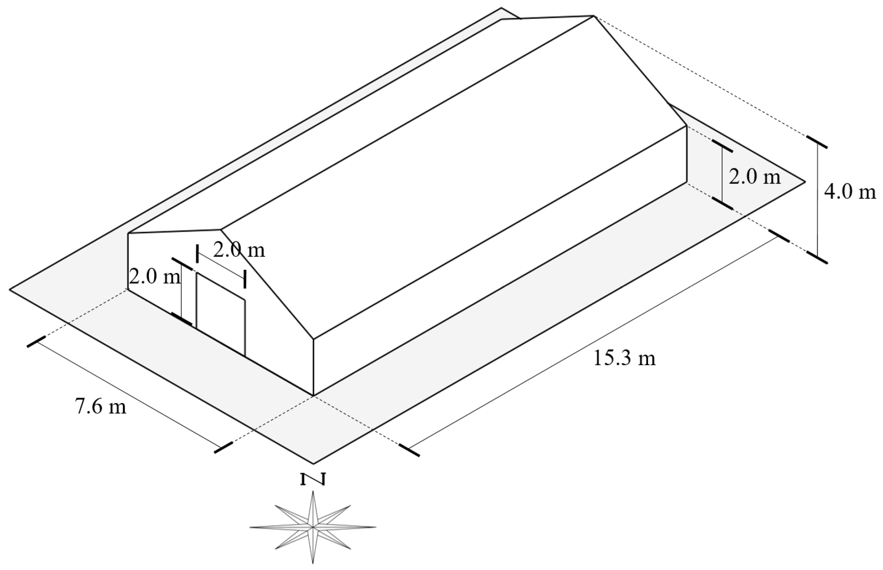
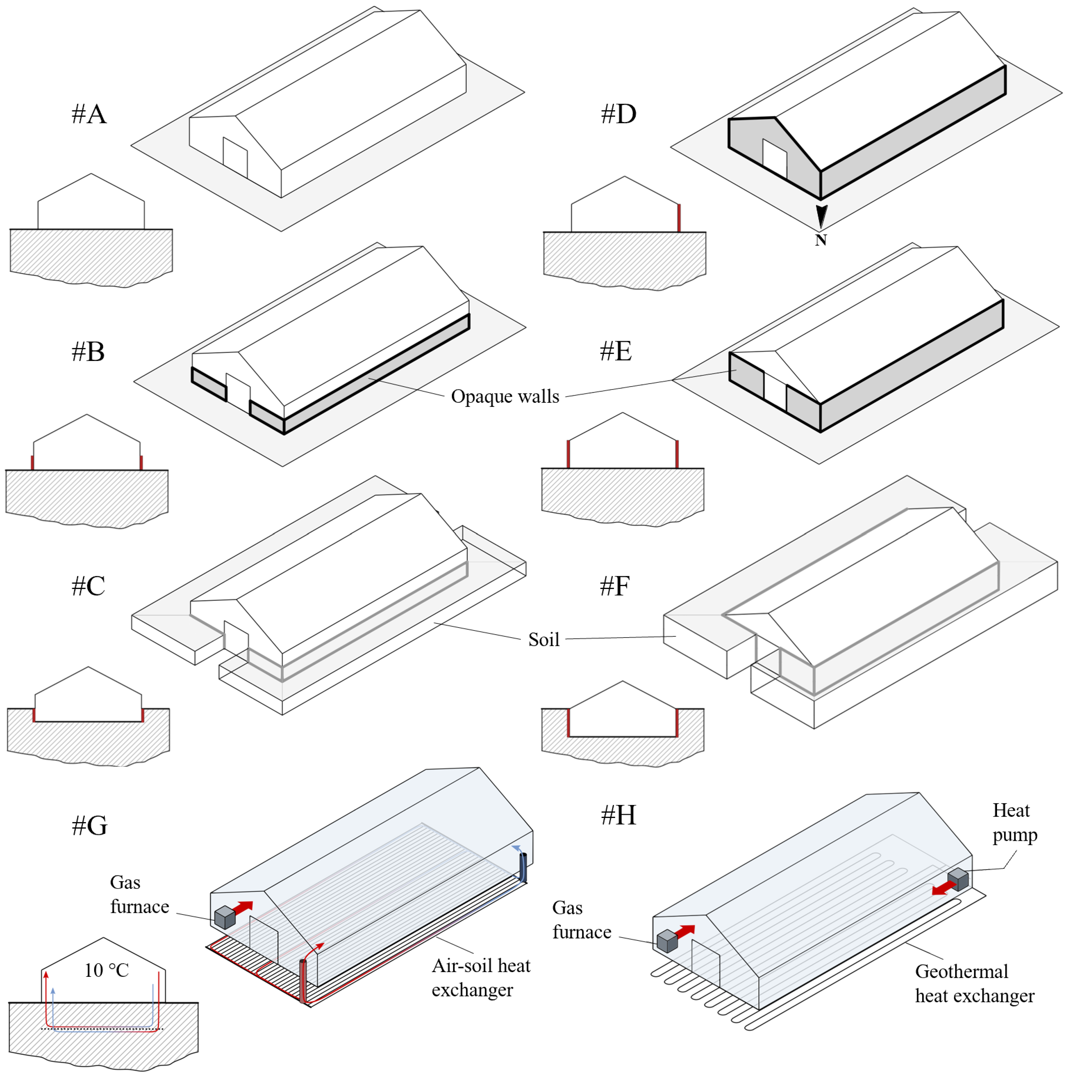
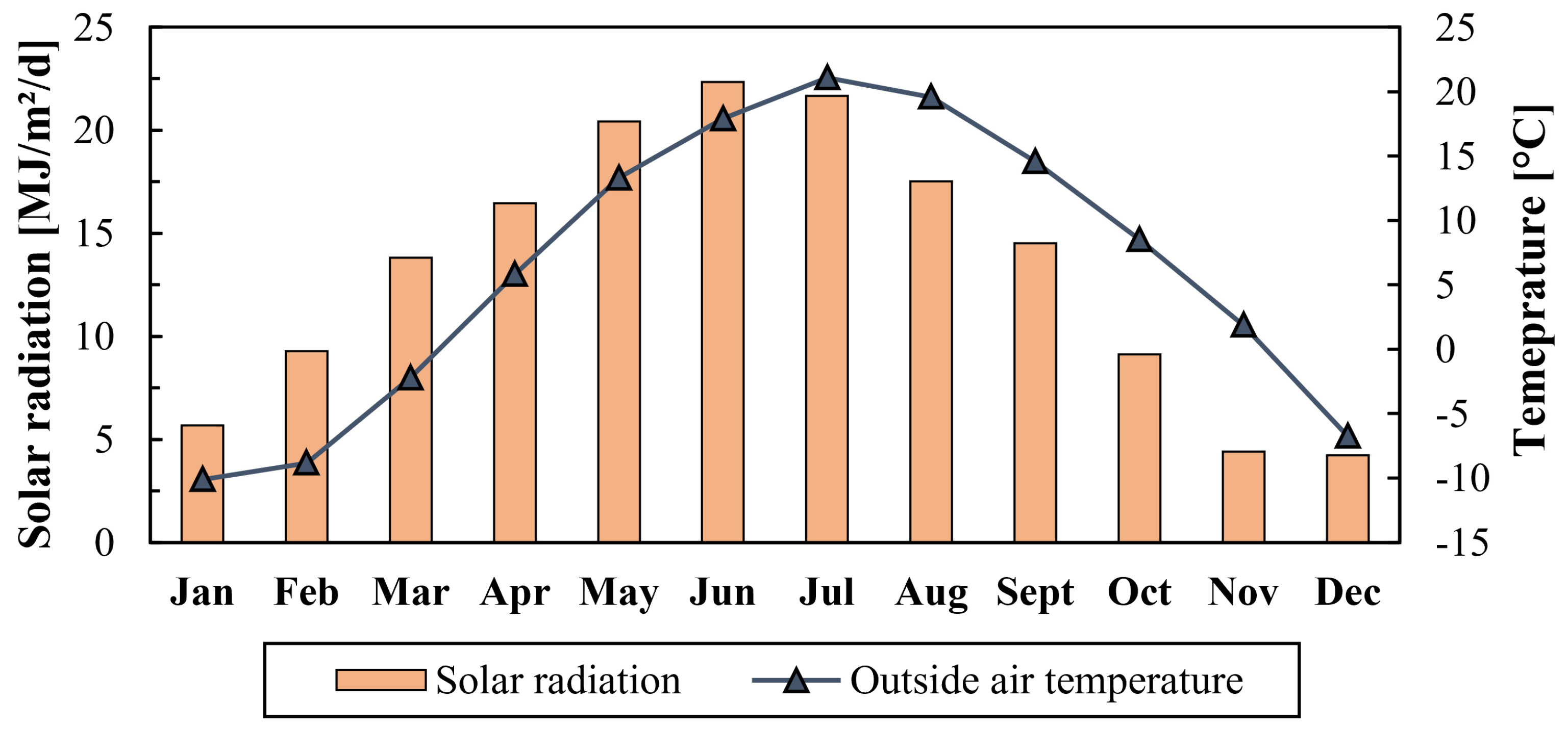
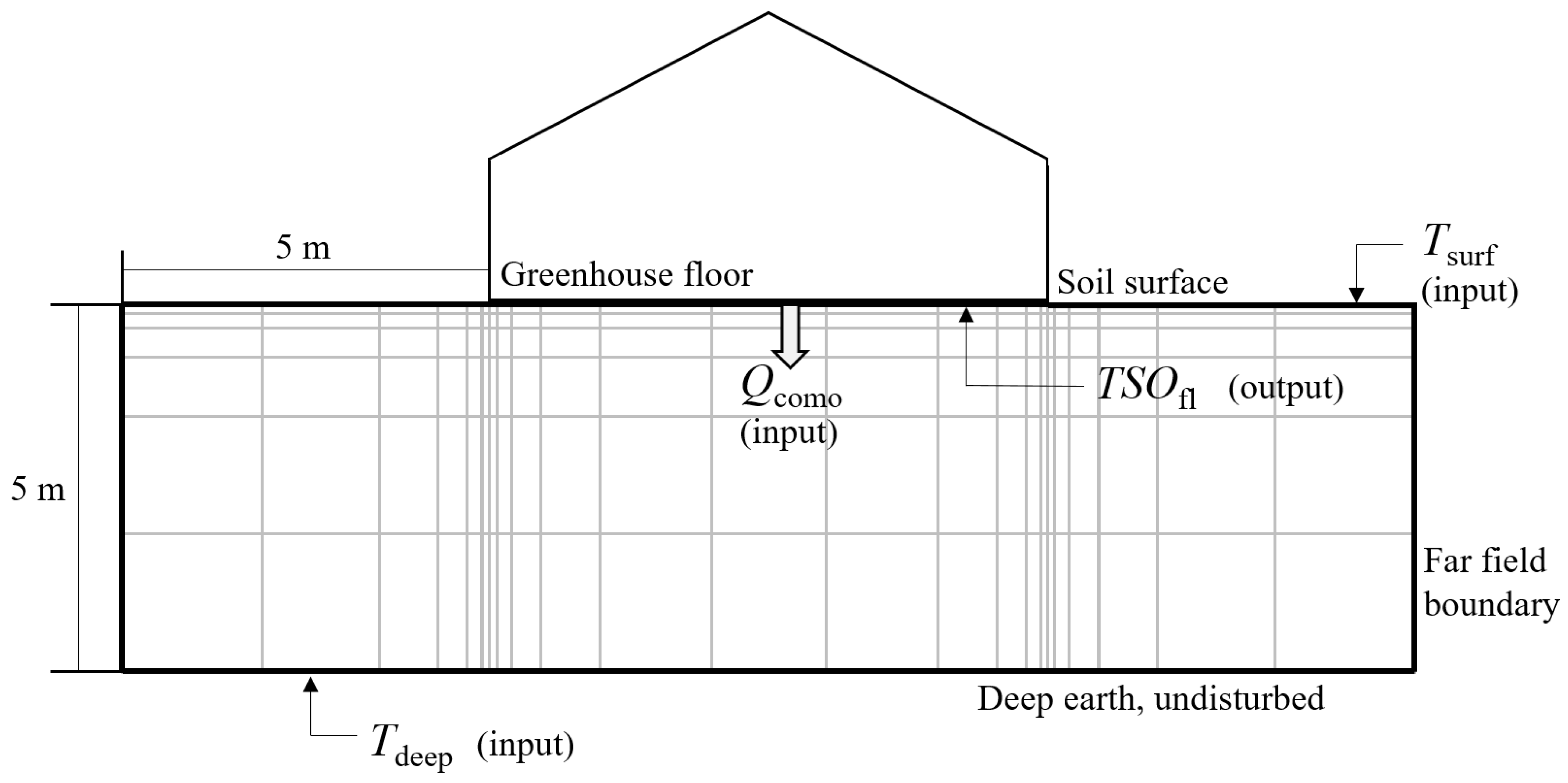
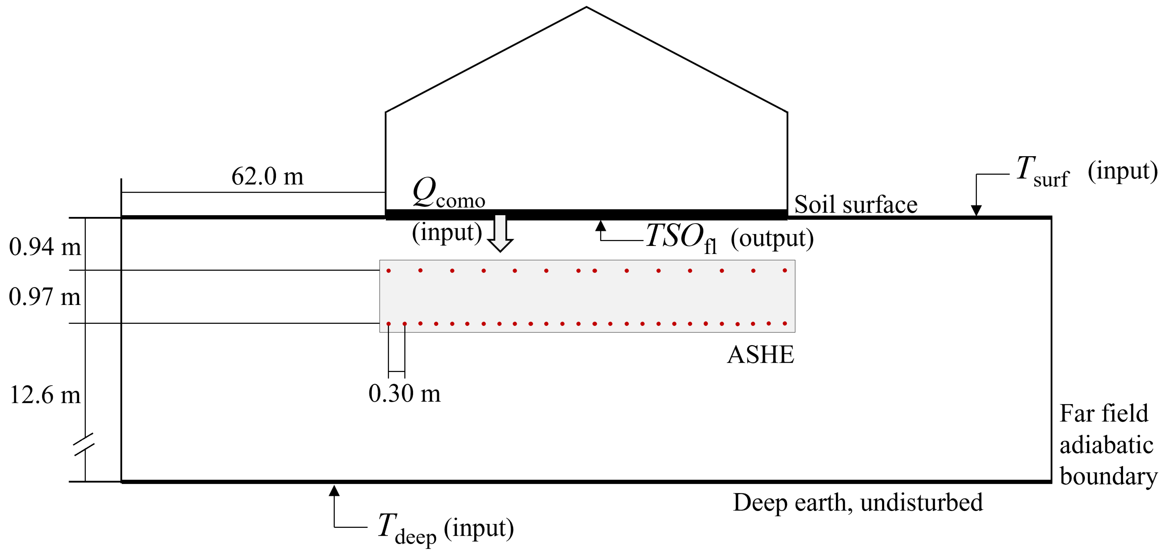
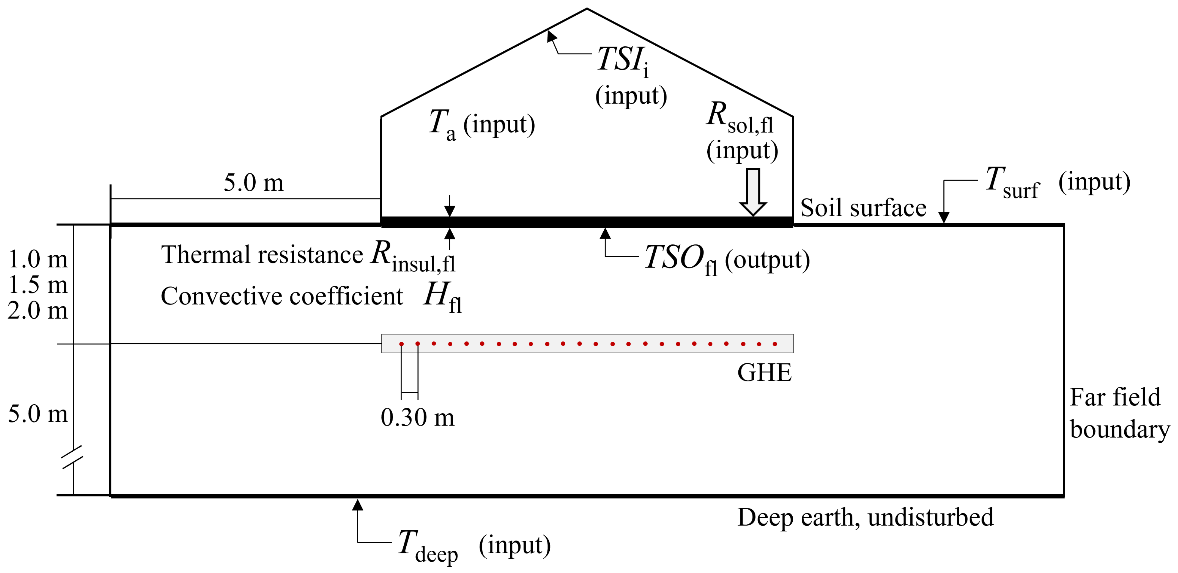
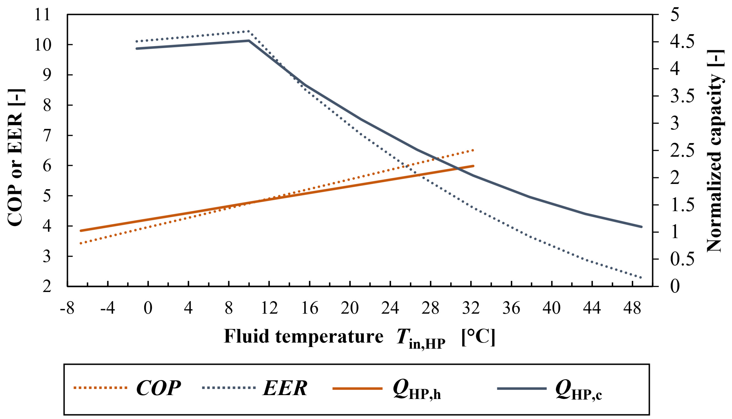
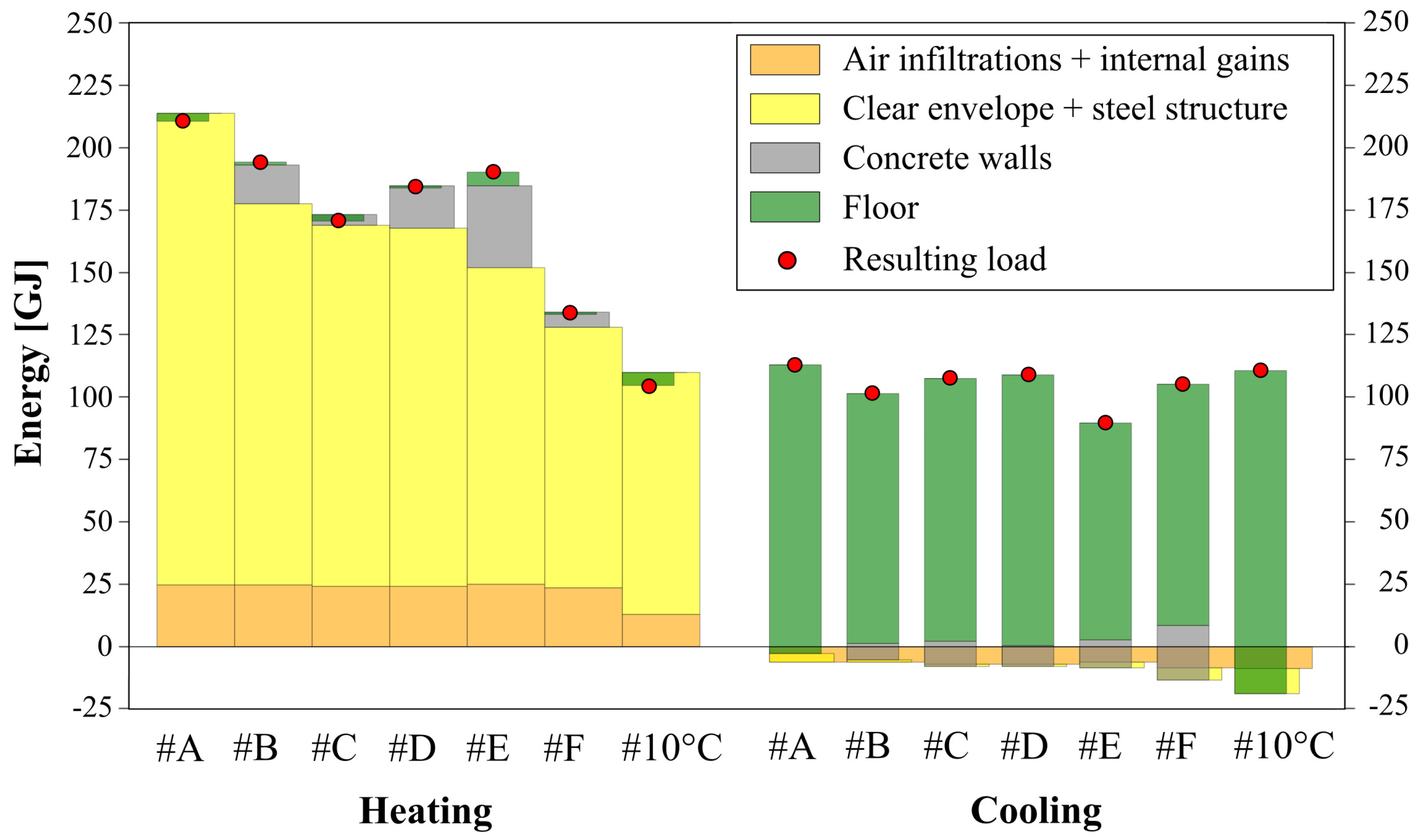
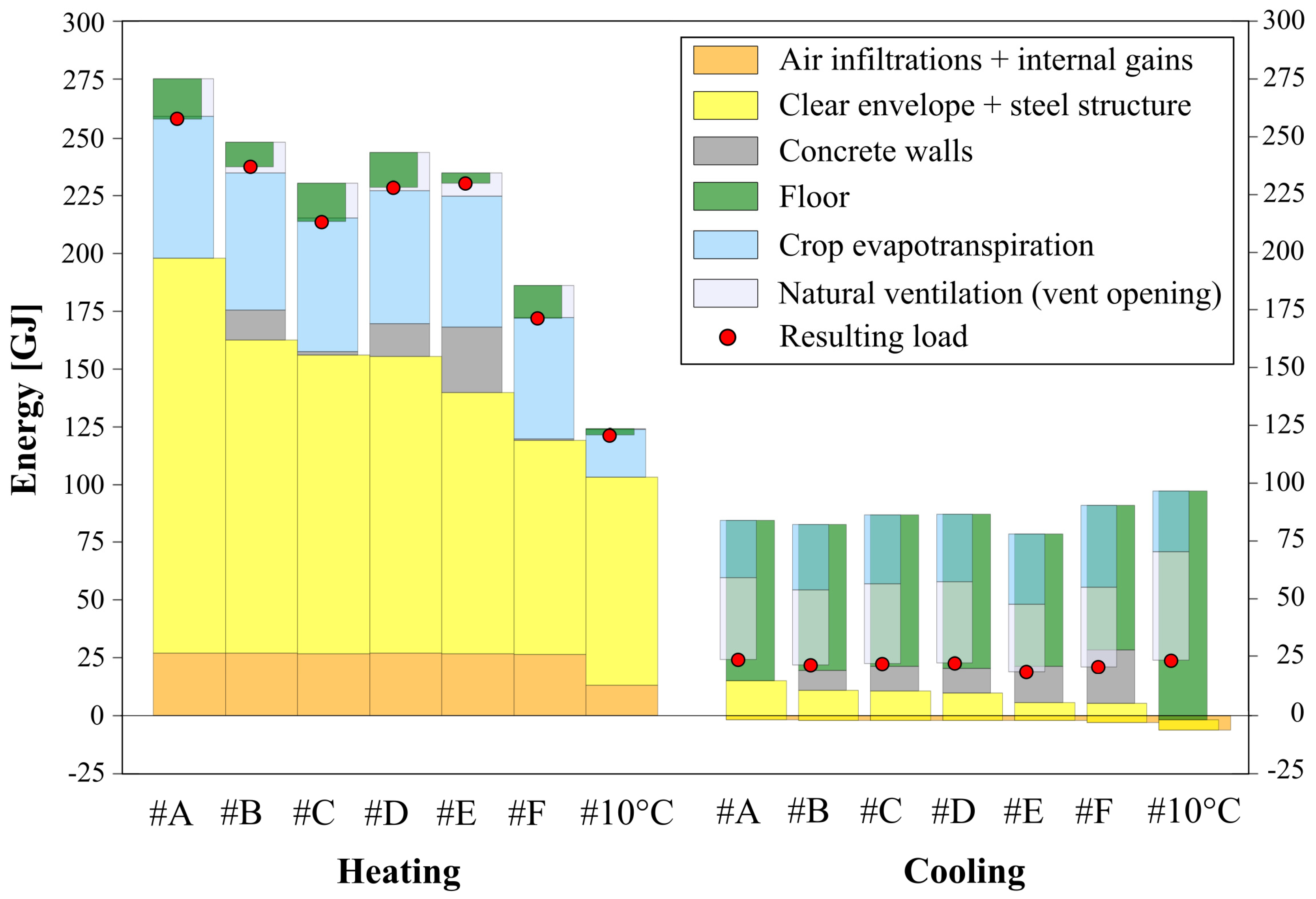
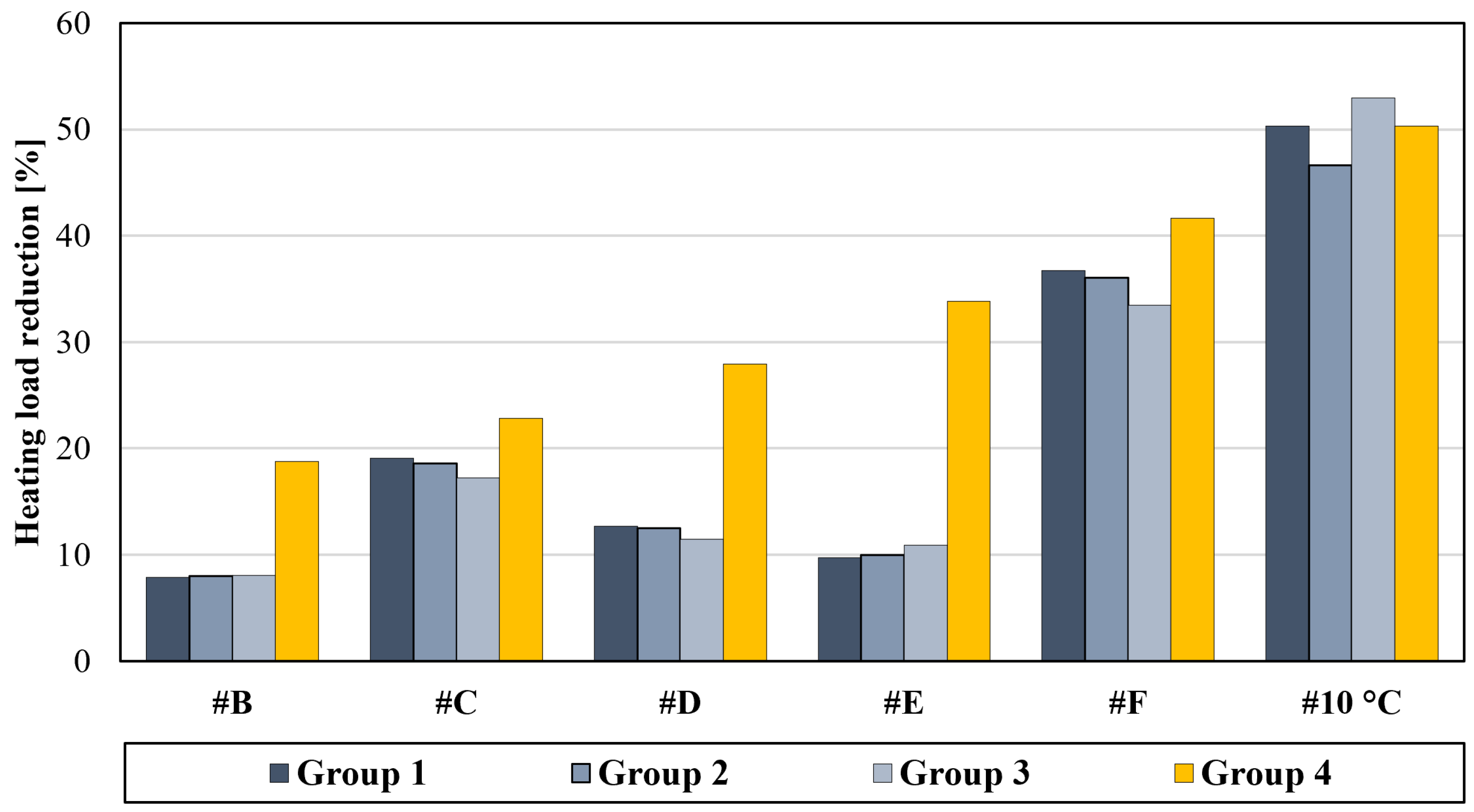
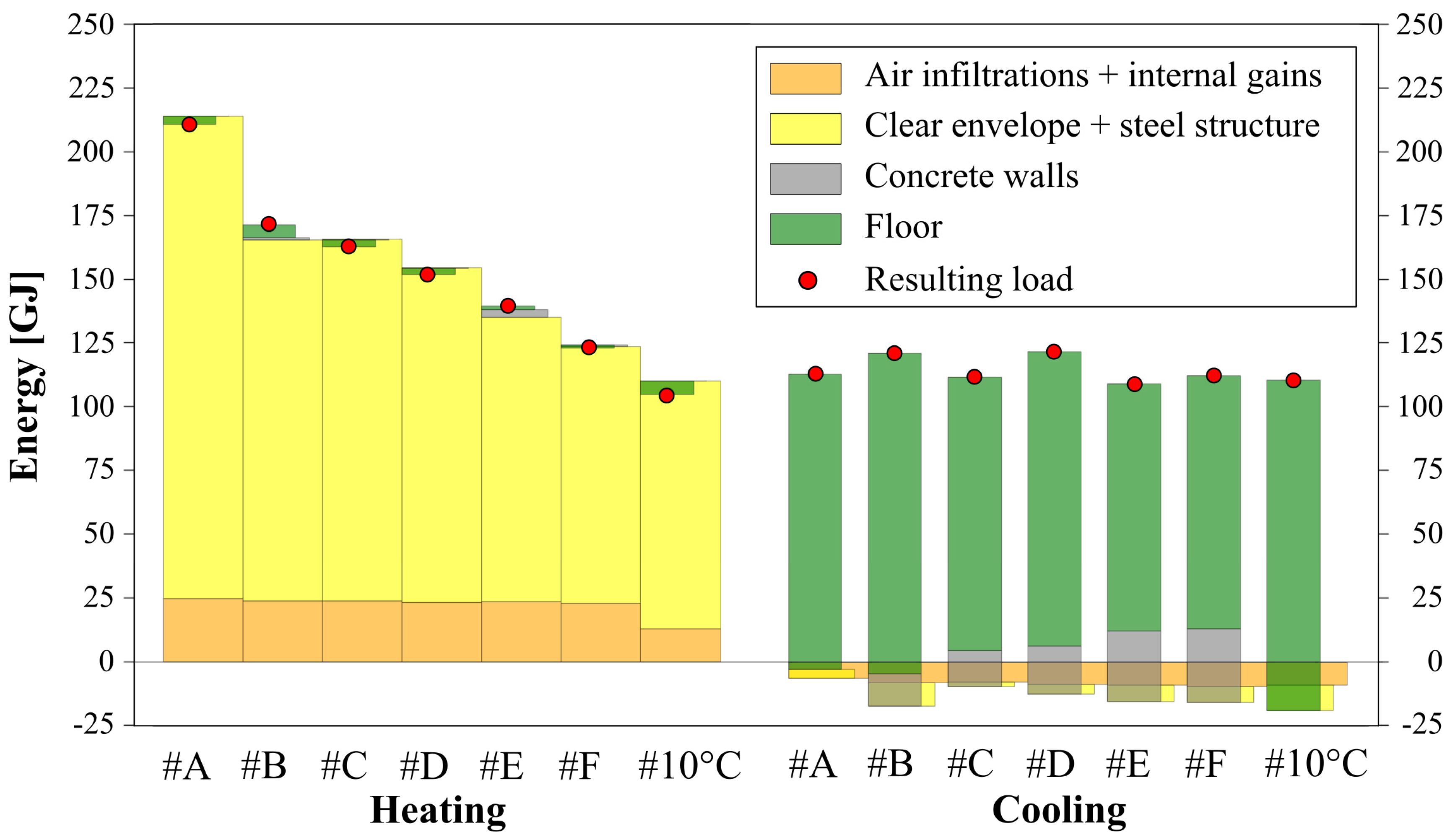
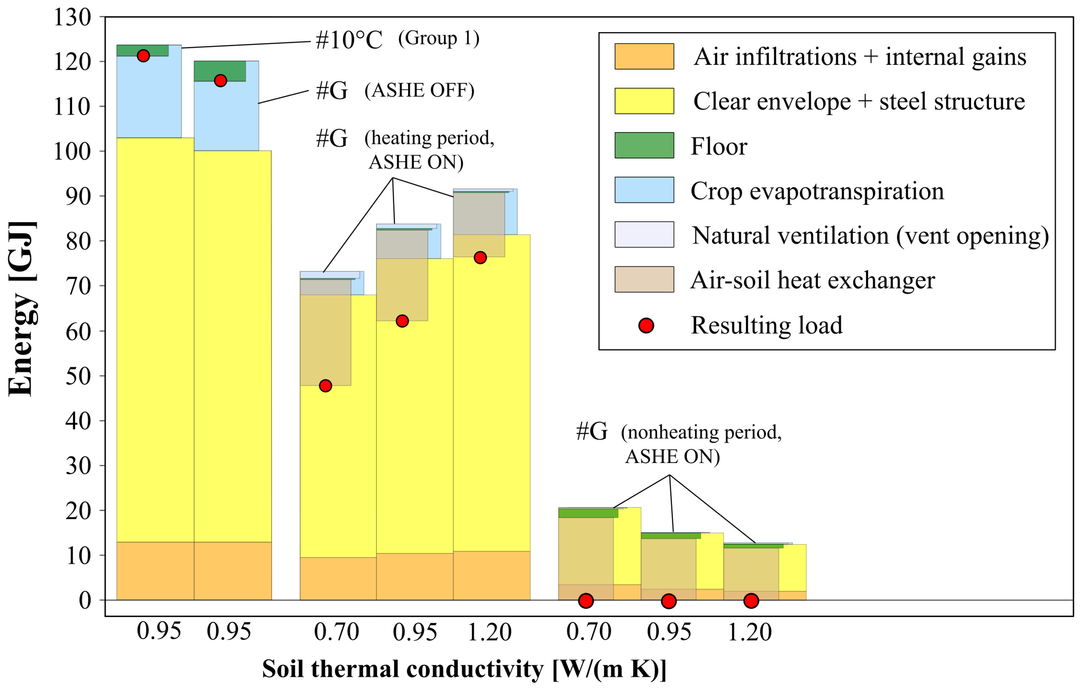
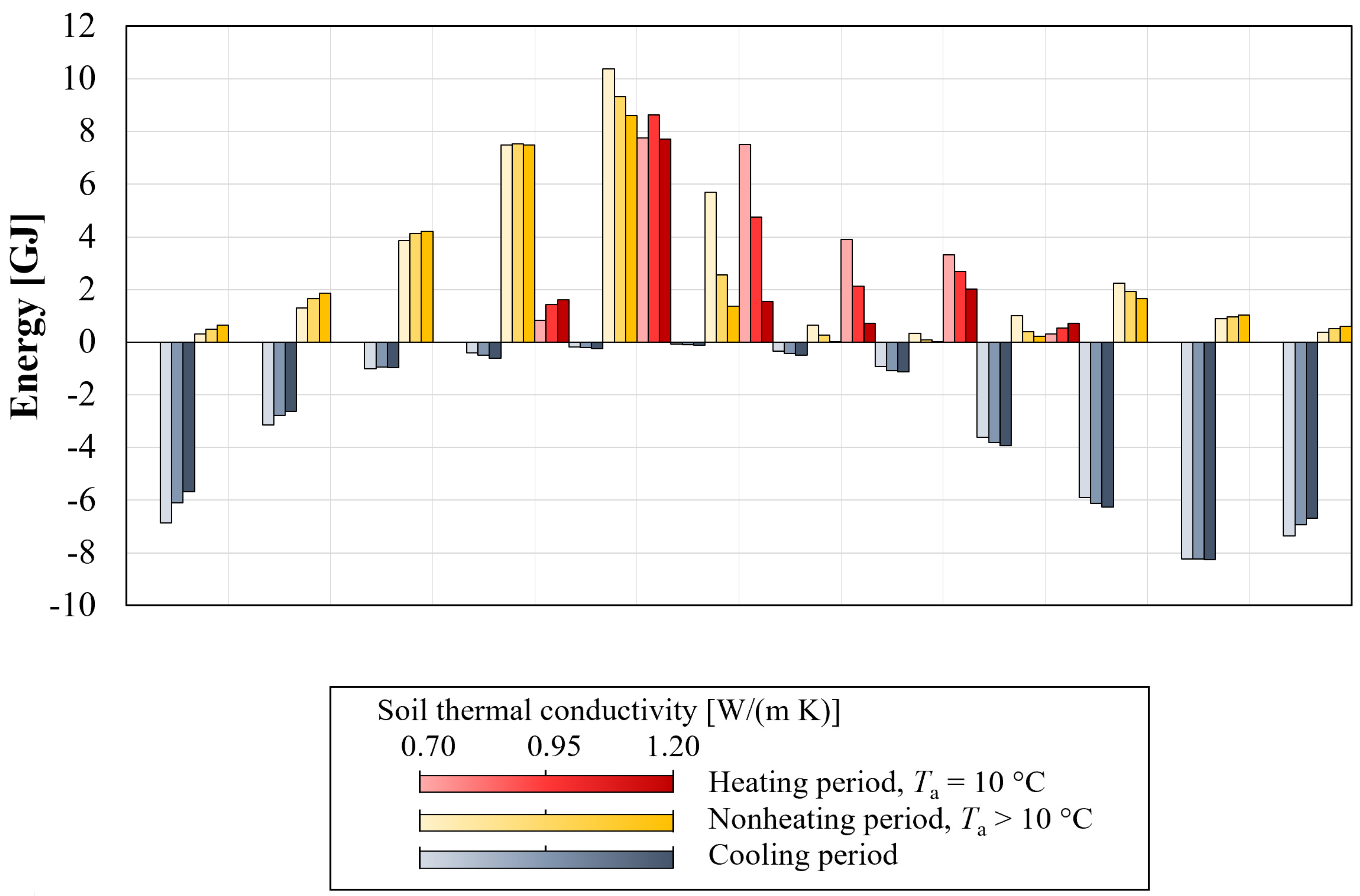
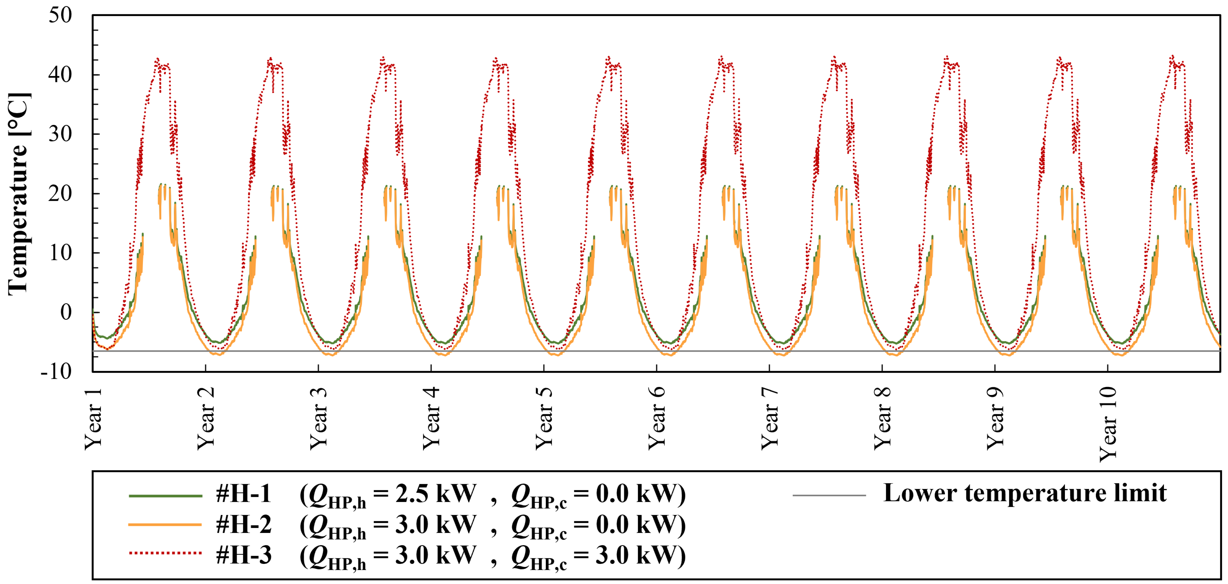
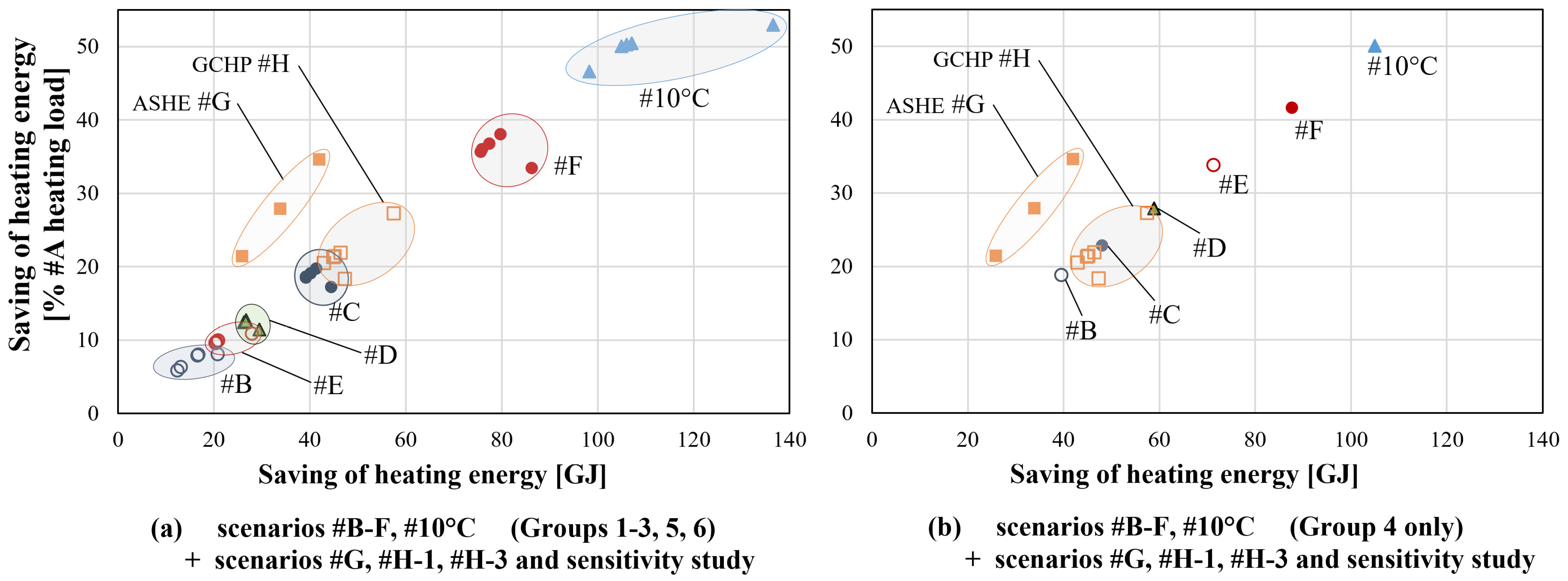
Table 1.
Thermal and radiative properties of the opaque elements of the greenhouse envelope.
| Layer | Total Thickness [m] | Thermal Resistance [m2 K/W] | Internal Convective Coefficient [W/(m2 K)] | External Convective Coefficient [W/(m2 K)] | Solar Absorptance in [−] | Solar Absorptance out [−] | Long-Wave Emission Coefficient in [−] | Long-Wave Emission Coefficient out [−] |
|---|---|---|---|---|---|---|---|---|
| Steel structure | 0.05 | 0.003 | 3.06 | He | 0.8 | 0.8 | 0.28 | 0.28 |
| Floor | − | 0.10 | Parametric study | − | 0.9 | 0.9 | 0.8 | 0.8 |
| Concrete wall (not insulated) | 0.20 | 0.21 | 3.06 | 17.8 | 0.6 | 0.6 | 0.9 | 0.9 |
| Concrete wall (with insulation) | 0.30 | 2.71 | 3.06 | 17.8 | 0.6 | 0.6 | 0.9 | 0.9 |
| Plywood door | 0.05 | 0.33 | 3.06 | 17.8 | 0.6 | 0.6 | 0.9 | 0.9 |
Table 2.
Thermal and radiative properties of the clear elements of the greenhouse envelope.
| Glazing | Frame | Convective Heat Transfer Coefficient | ||||||||
|---|---|---|---|---|---|---|---|---|---|---|
| Windows | Slope [deg] | U-Value (Convection not Included) [W/(m2 K)] | g [−] | τsol [−] | ρsol [−] | U-Value [W/(m2 K)] | Solar Absorptance [−] | Emissivity [−] | Internal [W/(m2 K)] | External [W/(m2 K)] |
| PE 90° (side walls) | 90 | 4.38 | 0.773 | 0.747 | 0.175 | 8.17 | 0.6 | 0.9 | Parametric study | He |
| PE 28° (roof) | 28 | 4.28 | 0.775 | 0.747 | 0.175 | 8.17 | 0.6 | 0.9 | Parametric study | He |
| PC (front–back walls) | 90 | 3.64 | 0.671 | 0.62 | 0.227 | 8.17 | 0.6 | 0.9 | Parametric study | He |
Table 3.
Parameters of the evapotranspiration model.
| Parameter | Value | Unit | Additional Information |
|---|---|---|---|
| Cp | 1006 | J/(kg K) | − |
| fcult | 0.6 | − | The crops cover 60% of the floor surface area. |
| ks | 0.66 | − | Coefficient of extinction reported by Tei et al. (1996) for lettuce. Crops, with cultivated density of 27.5 plants/m2 [32]. |
| LAI | 3.0 | − | Presumed by Graamans et al. (2017) for lettuce crops, based on literature [23,29]. |
| λ | 2489 | kJ/kg | − |
| γ | 66.5 | Pa/K | − |
| ρa | 1.2 | kg/m3 | The density of humid air lies between 1.18 and 1.23 kg/m3 according to the simulated temperature and relative humidity. |
Table 4.
ASHE, GHE, and HP model parameters for scenarios #G, H.
| Component | Parameter | Unit | Value |
|---|---|---|---|
| ASHE: Type 460 Scenario #G | Total air flow rate | m3/s | 0.83 |
| Number of pipes (all in parallel connection) | − | 40 | |
| Pipe inner diameter | m | 0.08 | |
| Pipe outer diameter | m | 0.09 | |
| Single pipe length | m | 15.0 | |
| Pipe spacing | m | 0.3 | |
| Burial depth of pipes | m | 0.9 and 1.9 | |
| Pipe thermal conductivity | W/(m K) | 2.0 | |
| Pipe heat capacity | MJ/(m3 K) | 1.0 | |
| Soil thermal conductivity | W/(m K) | Parametric study | |
| Soil heat capacity | MJ/(m3 K) | 2.25 | |
| GHE: Type 997 Scenario #H | Number of pipes (all in serial connection) | − | 24 |
| Pipe inner diameter | m | 0.019 | |
| Pipe outer diameter | m | 0.024 | |
| Single pipe length | m | 15.0 | |
| Pipe spacing | m | 0.30 | |
| Burial depth of pipes | m | Parametric study | |
| Pipe thermal conductivity | W/(m K) | 0.4 | |
| Pipe heat capacity | W/(m K) | 0.95 | |
| Soil thermal conductivity | W/(m K) | Parametric study | |
| Soil heat capacity | MJ/(m3 K) | 2.25 | |
| HP: Equations Scenario #H | Rated heating capacity | kW | Parametric study |
| Rated cooling capacity | kW | Parametric study | |
| Heat carrier fluid (volume mixture of 65% water + 35% propylene glycol) Scenario #H | Specific heat capacity | kJ/(kg K) | 3.726 |
| Density | kg/m3 | 1037 | |
| Thermal conductivity | W/(m K) | 0.4 | |
| Volume flow rate | L/s | 0.28 | |
| Dynamic viscosity | kg/(m h) | 33 |
Table 5.
Characteristics of the groups of models considered in the parametric study.
| Group 1 #A–F, H, 10 °C | Group 2 #A–F, 10 °C | Group 3 #A–F, H, 10 °C | Group 4 #A–F, 10 °C | Group 5 #A–F, H, 10 °C | Group 6 #A–F, H, 10 °C | |
|---|---|---|---|---|---|---|
| Calculation of internal convective coefficient | Equations (2) and (3) | Hin,i of scenario #A, calculated with Equations (2) and (3) | Equations (2) and (3) | Equations (2) and (3) | Equations (2) and (3) | Equations (2) and (3) |
| Evapotranspiration | no | no | yes | no | no | no |
| Condensation | no | no | yes | no | no | no |
| Natural ventilation | no | no | yes | no | no | no |
| Concrete wall thermal resistance [m2 K/W] | 0.21 (no insulation) | 0.21 (no insulation) | 0.21 (no insulation) | 2.71 (with insulation) | 0.21 (no insulation) | 0.21 (no insulation) |
| Soil thermal conductivity [W/(m K)] | 0.95 | 0.95 | 0.95 | 0.95 | 0.7 | 1.2 |
Table 6.
Heat transferred from the ASHE to the zone during the heating, nonheating, and cooling periods.
Table 6.
Heat transferred from the ASHE to the zone during the heating, nonheating, and cooling periods.
| Soil Thermal Conductivity [W/(m K)] | Heat from ASHE to Zone during Heating Period [GJ] | Heat from ASHE to Zone during Nonheating Period [GJ] | Heat from ASHE to Zone during Cooling Period [GJ] | ||
|---|---|---|---|---|---|
| Total | Part Contributing to Saving | Total | Part Contributing to Saving | Total (Soil Heat Injection) | |
| 0.70 | 23.6 | 23.6 | 34.6 | 18.4 | −38.2 |
| 0.95 | 20.2 | 20.2 | 29.9 | 13.7 | −37.4 |
| 1.20 | 14.3 | 14.3 | 27.8 | 11.6 | −37.2 |
Table 7.
Ground peak load related to heating and cooling, during a ten-year operation, for scenarios #H-1, #H-2, and #H-3, for a soil thermal conductivity of 0.95 W/(m K) and a GHE depth of 1.5 m (Group 1 models).
Table 7.
Ground peak load related to heating and cooling, during a ten-year operation, for scenarios #H-1, #H-2, and #H-3, for a soil thermal conductivity of 0.95 W/(m K) and a GHE depth of 1.5 m (Group 1 models).
| QHP,h – QHP,c [kW] | Maximum Yearly Ground Load (Heating) [W] | Maximum Monthly Ground Load (Heating) [W] | Maximum Hourly Ground Load (Heating) [W] | Minimum Fluid Temperature Tmin,in,HP [°C] |
|---|---|---|---|---|
| 2.5–0.0 (#H-1) | 1187.4 | 2302.1 | 3474.9 | −5.3 |
| 3.0–0.0 (#H-2) | 1326.1 | 2689.4 | 3948.5 | −7.3 |
| 3.0–3.0 (#H-3) | 16.8 | 2919.1 | 5300.0 | −6.2 |
Table 8.
Yearly heating and cooling loads, heat provided by the HP, and electrical energy consumed by the HP during an average year of the ten-year operation for a soil thermal conductivity of 0.95 W/(m K) and a GHE depth of 1.5 m (Group 1 models).
Table 8.
Yearly heating and cooling loads, heat provided by the HP, and electrical energy consumed by the HP during an average year of the ten-year operation for a soil thermal conductivity of 0.95 W/(m K) and a GHE depth of 1.5 m (Group 1 models).
| QHP,h − QHP,c [kW] | Yearly Heating Load [GJ] | Yearly Cooling Load [GJ] | EHP→zone Heating [GJ] | EHP→zone Cooling [GJ] | Eelec,HP Heating [GJ] | Eelec,HP Cooling [GJ] |
|---|---|---|---|---|---|---|
| 2.5–0.0 (#H-1) | 215.5 | 115.6 | 49.7 | 0.0 | 12.7 | 0.0 |
| 3.0–0.0 (#H-2) | 216.3 | 115.3 | 56.0 | 0.0 | 14.9 | 0.0 |
| 3.0–3.0 (#H-3) | 212.6 | 121.9 | 59.3 | −32.6 | 14.5 | 11.6 |
Table 9.
Fraction of the heating and cooling loads provided by the HP, final energy savings, and minimum fluid temperature in scenario #H during a ten-year operation for a soil thermal conductivity of 0.95 W/(m K) and a GHE depth of 1.5 m (Group 1 models).
Table 9.
Fraction of the heating and cooling loads provided by the HP, final energy savings, and minimum fluid temperature in scenario #H during a ten-year operation for a soil thermal conductivity of 0.95 W/(m K) and a GHE depth of 1.5 m (Group 1 models).
| QHP,h – QHP,c [kW] | Fraction of the Heating Load Provided by the HP [%] | Fraction of the Cooling Load Provided by the HP [%] | Savings in Heating Energy [% of #A Heating Load, Group 1] | Savings in Cooling Energy [% of #A Cooling Load, Group 1] | Minimum Fluid Temperature Tmin,in,HP [°C] |
|---|---|---|---|---|---|
| 2.5–0.0 (#H-1) | 23.1 | 0.0 | 21.3 | 2.7 | −5.3 |
| 3.0–0.0 (#H-2) | 25.9 | 0.0 | 23.8 | 2.9 | −7.3 |
| 3.0–3.0 (#H-3) | 27.9 | 26.7 | 27.3 | 24.8 | −6.2 |
Table 10.
Summary of HP performance and energy savings depending on the soil thermal conductivity and the GHE depth, for scenario #H-1 and its associated parametric study, during an average year of the ten-year operation.
Table 10.
Summary of HP performance and energy savings depending on the soil thermal conductivity and the GHE depth, for scenario #H-1 and its associated parametric study, during an average year of the ten-year operation.
| Soil Thermal Conductivity [W/(m K)] | GHE Depth [m] | Yearly Heating Load [GJ] | EHP→zone [GJ] | Eelec,HP [GJ] | Fraction of the Heating Load Provided by the HP [%] | Savings in Heating Energy [% of #A Heating Load, Groups 1, 3, 5, or 6] | Minimum Fluid Temperature Tmin,in,HP [°C] |
|---|---|---|---|---|---|---|---|
| 0.95 * (Group 1) | 1.5 * | 215.5 | 49.7 | 12.7 | 23.1 | 21.3 | −5.3 |
| 0.70 (Group 5) | 1.5 | 213.4 | 46.7 | 12.5 | 21.9 | 20.5 | −7.8 |
| 1.20 (Group 6) | 1.5 | 217.6 | 51.8 | 12.8 | 23.8 | 21.9 | −3.5 |
| 0.95 (Group 1) | 1.0 | 218.1 | 52.2 | 12.8 | 23.9 | 21.3 | −3.9 |
| 0.95 (Group 1) | 2.0 | 213.7 | 48.1 | 12.6 | 22.5 | 21.4 | −6.5 |
| 0.95 ** (Group 3) | 1.5 ** | 263.9 | 53.3 | 13.8 | 20.2 | 18.3 | −5.6 |
* Scenario #H-1. ** Group 3 models (with evapotranspiration, condensation, and natural ventilation).
Table 11.
Summary of simulation results available in the literature *.
| Reference and Equivalent Studied Scenario | Solution | Base Case Heating Load [GJ/y] | Allowed Savings [GJ] | Allowed Savings [% of Base Case Load] | Place | Remarks |
|---|---|---|---|---|---|---|
| Léveillé-Guillemette et al. (2018) [14] | Insulation of northwest wall with 10 cm expanded polystyrene layer | 209.3 | 14.7–16.7 | 7–8 | Emily- De-Witt greenhouse, Montreal | TRNSYS 18 software No condensation and no evapotranspiration One wall insulated |
| Scenario #D (Group 1) | Insulation of northwest and northeast walls with 20 cm concrete wall | 210.8 | 26.6 | 12.6 | − | TRNSYS 18 software Two walls insulated |
| Scenario #D (Group 3) | Insulation of northwest and northeast walls with 20 cm concrete wall | 257.9 | 29.5 | 11.4 | ||
| Scenario #D (Group 4) | Insulation of northwest and northeast walls with 20 cm concrete wall and 10 cm expanded polystyrene layer | 210.8 | 58.9 | 27.9 | ||
| Nawalany et al. (2017) [21] | Earth-sheltered greenhouse 1 m below ground surface, 30 cm concrete walls | 842.4 | 93.6 | 11 | South Poland (50.1° N, 19.5° E) | WUFI Plus software Greenhouse footprint 10.6 m × 43 m, height 4.3 m No condensation and no evapotranspiration Temperature range 17 °C–27 °C |
| Nawalany et al. (2017) [21] | Earth-sheltered greenhouse 1 m below ground surface, 30 cm concrete walls | 237.6 | 32.4 | 13.6 | (50.1° N, 19.5° E) | Temperature range 8 °C–24 °C |
| Scenario #C (Group 1) | 1 m below ground surface, 20 cm concrete walls | 210.8 | 40.2 | 19.1 | − | TRNSYS 18 software |
| Scenario #C (Group 3) | 1 m below ground surface, 20 cm concrete walls | 257.9 | 44.5 | 17.2 | ||
| Nawalany et al. (2017) [21] | Earth-sheltered greenhouse 1 m below ground surface, 30 cm concrete walls, insulation of 10 cm extruded polystyrene layer | 842.4 | 172.8 | 20.5 | South Poland (50.1° N, 19.5° E) | WUFI Plus software Greenhouse footprint 10.6 m × 43 m, height 4.3 m No condensation and no evapotranspiration Temperature range 17 °C–27 °C |
| Nawalany et al. (2017) [21] | Earth-sheltered greenhouse 1 m below ground surface, 30 cm concrete walls, insulation of 10 cm extruded polystyrene layer | 237.6 | 54 | 22.7 | (50.1° N, 19.5° E) | Temperature range 8 °C–24 °C |
| Scenario #C (Group 4) | 1 m below ground surface, 20 cm concrete walls, insulation of 10 cm expanded polystyrene | 210.8 | 48.1 | 22.8 | − | TRNSYS software |
* Table structure: Each case studied from the literature must be compared with the equivalent studied scenarios reported in the next lines. The thicker lines of the table indicate the beginning of a new set of studied cases to be compared.
Disclaimer/Publisher’s Note: The statements, opinions and data contained in all publications are solely those of the individual author(s) and contributor(s) and not of MDPI and/or the editor(s). MDPI and/or the editor(s) disclaim responsibility for any injury to people or property resulting from any ideas, methods, instructions or products referred to in the content. |
© 2023 by the authors. Licensee MDPI, Basel, Switzerland. This article is an open access article distributed under the terms and conditions of the Creative Commons Attribution (CC BY) license (https://creativecommons.org/licenses/by/4.0/).
Share and Cite
MDPI and ACS Style
Maranghi, F.; Raymond, J. Numerical Evaluation of the Benefits Provided by the Ground Thermal Inertia to Urban Greenhouses. Thermo 2023, 3, 452-482. https://doi.org/10.3390/thermo3030028
AMA Style
Maranghi F, Raymond J. Numerical Evaluation of the Benefits Provided by the Ground Thermal Inertia to Urban Greenhouses. Thermo. 2023; 3(3):452-482. https://doi.org/10.3390/thermo3030028
Chicago/Turabian StyleMaranghi, Florian, and Jasmin Raymond. 2023. "Numerical Evaluation of the Benefits Provided by the Ground Thermal Inertia to Urban Greenhouses" Thermo 3, no. 3: 452-482. https://doi.org/10.3390/thermo3030028