Fractional Bernoulli and Euler Numbers and Related Fractional Polynomials—A Symmetry in Number Theory

Abstract

Bernoulli and Euler numbers and polynomials are well known and find applications in various areas of mathematics, such as number theory, combinatorial mathematics, series expansions, and the theory of special functions. Using fractional exponential functions, we extend the classical Bernoulli and Euler numbers and polynomials to introduce their fractional-index-based types. This reveals a symmetry in relation to the classical numbers and polynomials. We demonstrate some examples of these generalized mathematical entities, which we derive using the computer algebra system Mathematica©.

1. Introduction

The study of fractional derivatives and their applications has been a topic of interest for many scholars. Their importance has only increased as they are used in various scientific fields. In the book written by S. Samko, A.A. Kilbas, and O. Marichev [1], the authors examine and compare different definition types of fractional differentiation. They also showcase the applications of fractional calculus in ordinary and partial differential equations. Other resources that one can refer to are the book by A.A. Kilbas, H.M. Srivastava, and J.J. Trujillo [2], the works by Gorenflo and Mainardi [3], and the article by Mainardi et al. [4].

Recently, an elementary approach based on Euler’s classical definition has been considered in [5,6]. The interested reader could find a similar technique in the articles by M. Ortigueira et al. [7,8,9], articles that were recently sent to us by the author, after the publication of our paper on symmetry [6]. These works are interesting since they clarify old and new definitions of the fractional derivative and find applications in the framework of the Laplace transform.

Our method falls under Caputo’s [10] and utilizes power series with a fractional exponent. Using this method, it is possible to extend classical polynomials and the associated special numbers to the case of fractional indices. As known from theory, Euler and Bernoulli numbers appear in the Taylor series expansions of trigonometric and hyperbolic functions. They also occur in combinatorics as well as in the computation of special functions, such as the Riemann zeta function.

Fractional Bernoulli numbers and polynomials have recently been considered by E. Woldeyohannes [11], starting from the following generating functions:

• For the fractional numbers $B_{\alpha ,k}$, where $\alpha$ is a fractional number,

  $$\begin{array}{c}\hfill {\displaystyle \frac{x^{2\alpha }{e}^{-x^2}}{\alpha \gamma (\alpha ,x^2)}=\sum _{k=0}^{\infty }{B}_{\alpha ,k}\frac{x^k}{k!},}\end{array}$$
• For the fractional polynomials $B_{\alpha ,k}\left(z\right)$,

  $$\begin{array}{c}\hfill {\displaystyle \frac{x^{2\alpha }{e}^{xz-x^2}}{\alpha \gamma (\alpha ,x^2)}=\sum _{k=0}^{\infty }{B}_{\alpha ,k}\left(z\right)\frac{x^k}{k!},}\end{array}$$

  where $\gamma (a,x)={\int }_0^x{e}^{-t}{t}^{\alpha -1}dt$ denotes the lower incomplete gamma function.

Our purpose in this paper is to introduce fractional Bernoulli numbers and polynomials by using a completely different approach. In fact, in a recent article [6], we have introduced a fractional version of the exponential function by posing

$$\begin{array}{c}\hfill {\displaystyle {\mathrm{Exp}}_{\alpha }\left(t\right)=1+\frac{t^{\alpha }}{\Gamma (\alpha +1)}+\frac{t^{2\alpha }}{\Gamma (2\alpha +1)}+\cdots +\frac{t^{n\alpha }}{\Gamma (n\alpha +1)}+\cdots ,}\end{array}$$

(1)

and we use this function, expanded in fractional powers, in the generating function of the fractional form of the Bernoulli numbers and polynomials [12]. Note that the fractional exponential function above is a true exponential with respect to the operator $D_x^{\alpha }$ since it satisfies the following eigenvalue properties:

$$\begin{array}{c}\hfill D_t^{\alpha }{\mathrm{Exp}}_{\alpha }\left(xt\right)=x^{\alpha }{\mathrm{Exp}}_{\alpha }\left(xt\right),\end{array}$$

and

$$\begin{array}{c}\hfill D_x^{\alpha }{\mathrm{Exp}}_{\alpha }\left(xt\right)=t^{\alpha }{\mathrm{Exp}}_{\alpha }\left(xt\right).\end{array}$$

We have previously demonstrated potential applications of this function in various frameworks, such as fractional extensions of population dynamics problems, fractional Laplace transforms [13], and fractional Hermite polynomials [14].

It is important to note that the pseudo-exponential functions introduced in [15], which are generalized forms of exponential functions, are connected to the Mittag-Leffler function [16] and do not satisfy the eigenvalue property of the classical exponential, as explained in [13].

The fractional exponential function in (1) can be used to establish a special symmetry in number theory. For any value of $\alpha$ between 0 and 1, it is possible to generate a set of fractional index Bernoulli or Euler numbers and polynomials that correspond to the classical mathematical entities. These new sets of numbers are real numbers that depend on fractional indices. They are obtained by replacing the ordinary exponential function with the fractional exponential function in the generating function that defines the set of numbers or polynomials. This approach appears to be more natural than the one considered in [11].

It is worth noting that it is crucial to construct special functions that satisfy the eigenvalue property mentioned above with respect to suitable differential operators. This allows for the generalization of families of special numbers or polynomials using the same method employed in this article.

We have previously studied another type of function known as Laguerre-type exponentials. These functions have associated Laguerre-type special functions that create symmetry in the space of analytic functions. The operator $DxD=D+x{D}^2$ introduces a linear differential isomorphism that acts on the space of analytic functions of the variable x, creating a parallel structure within this space. This allows us to easily derive differentiation properties. Iterations of the Laguerre derivative can also create parallelism, leading to an endless cycle of construction within the space of analytic functions. This cyclic construction repeats the same structure at a higher level of differentiation order, showcasing the great cycles that can occur within mathematical theories. If one is interested in learning more, they can refer to the articles mentioned [17,18].

In Section 2, we review the generating function of Appell-type polynomials. In Section 3 and its relevant subsections, we introduce fractional indices Bernoulli numbers and fractional Bernoulli polynomials for a parameter $\alpha$ with a value between 0 and 1. We pay particular attention to the case where $\alpha =1/2$. We use the computer algebra system Mathematica© to derive several tables that show the convergence of these fractional entities to their corresponding classical ones as $\alpha$ approaches 1. In Section 4, we provide the same results and tables for fractional indices Euler numbers and fractional Euler polynomials. Our aim is to demonstrate, in a future article, the properties of classical numbers and polynomials that also apply to their fractional versions. While we could also study other forms of numbers and polynomials, such as Genocchi numbers and polynomials or Apostol-type polynomials, we limit ourselves to the Bernoulli and Euler cases to avoid overwhelming our readers.

Remark 1. 

Note that what we call fractional Bernoulli and Euler polynomials are actually functions, not polynomials in the strict sense, but since they are combinations of monomials with fractional powers, it seems more appropriate for us to retain the name polynomials as shorthand for fractional power polynomials.

2. Recalling the Fractional Appell-Type Polynomials

In this section, we consider first the fractional Appell polynomials depending on a fractional parameter $\alpha$, with $0<\alpha <1$, since the Bernoulli and Euler ones are a particular case of this more general class.

Using the Euler definition of fractional derivative

$$D^{\alpha }{x}^m:=\frac{d^{\alpha }{x}^m}{d{x}^{\alpha }}=\frac{\Gamma (m+1)}{\Gamma (m+1-\alpha )}{t}^{m-\alpha },(m\ge \left[\alpha \right]),$$

it is possible to define the fractional case of Appell polynomials. These are functions expressed by the combination of monomials with fractional powers, defined by the generating function that is obtained by substituting the fractional exponential of order $\alpha$ in place of the ordinary exponential in the corresponding classical generating function.

Definition 1. 

The fractional Appell-type polynomials of order α are defined by the following generating function:

$$\begin{array}{c}\hfill {\displaystyle G_{\alpha }(x,t)=A\left(t\right){\mathrm{Exp}}_{\alpha }\left(xt\right)=\sum _{n=0}^{\infty }{R}_{n\alpha }\left(x\right)\frac{t^{n\alpha }}{\Gamma (n\alpha +1)}.}\end{array}$$

In [13], the lowering operator for fractional Appell polynomials has been introduced in the particular case when $\alpha =1/2$, but the same result can be obtained for any fractional $\alpha$, with $0<\alpha <1$.

The following sections consider specific examples of this important family of polynomials, starting with the Bernoulli and Euler cases, based on their associated number sets.

3. Fractional Index Bernoulli Numbers and Polynomials

We introduce the following definitions:

1.

For the fractional index numbers $B_{\alpha ,k}$, where $\alpha$ is a fractional number,

$$\begin{array}{c}\hfill {\displaystyle \frac{x^{\alpha }}{{\mathrm{Exp}}_{\alpha }\left(x\right)-1}=\sum _{k=0}^{\infty }{B}_{\alpha ,k}\frac{x^{k\alpha }}{\Gamma (k\alpha +1)},}\end{array}$$

(2)

2.

For the fractional index polynomials $B_{\alpha ,k}\left(z\right)$,

$$\begin{array}{c}\hfill {\displaystyle \frac{x^{\alpha }{\mathrm{Exp}}_{\alpha }\left(xz\right)}{{\mathrm{Exp}}_{\alpha }\left(x\right)-1}=\sum _{k=0}^{\infty }{B}_{\alpha ,k}\left(z\right)\frac{x^{k\alpha }}{\Gamma (k\alpha +1)}.}\end{array}$$

(3)

3.1. Fractional Index Bernoulli Numbers

Introducing the definition (2) and posing, for convenience,

$$\begin{array}{c}\hfill {\delta }_{k,0}^c=1-{\delta }_{k,0},\end{array}$$

where ${\delta }_{k,0}$ is the Kronocher delta, so that ${\delta }_{k,0}^c=0,\mathrm{if}k=0$, and ${\delta }_{k,0}^c=1,\mathrm{if}k\ne 0$, we find

$$\begin{array}{c}\hfill {\displaystyle x^{\alpha }=\sum _{n=0}^{\infty }\frac{{\delta }_{k,0}^c{x}^{n\alpha }}{\Gamma (n\alpha +1)}\sum _{k=0}^{\infty }{B}_{\alpha ,k}\frac{x^{n\alpha }}{\Gamma (n\alpha +1)}}\end{array}$$

$$\begin{array}{c}\hfill {\displaystyle x^{\alpha }=\sum _{n=1}^{\infty }\sum _{k=1}^n\frac{x^{n\alpha }{B}_{\alpha ,n-k}}{\Gamma (k\alpha +1)\Gamma \left(\right(n-k)\alpha +1)}.}\end{array}$$

(4)

Equation (4) results in a triangular system of algebraic equations. Therefore, we can state the following theorem:

Theorem 1. 

The Bernoulli numbers with fractional indices $B_{\alpha ,k}$ can be sequentially computed by solving the triangular system

$$\begin{array}{c}{B}_{\alpha ,0}=\Gamma (\alpha +1),\hfill \\ {\displaystyle \sum _{k=1}^n}\frac{B_{\alpha ,n-k}}{\Gamma (k\alpha +1)\Gamma \left(\right(n-k)\alpha +1)}=0,\forall n\ge 1.\hfill \end{array}$$

(5)

3.2. The Fractional Index Bernoulli Numbers for $\alpha =1/2$

In order to fix the attention and give numerical examples, we consider the case when $\alpha =1/2$.

Equation (4) writes

$$\begin{array}{c}\hfill {\displaystyle x^{1/2}=\sum _{n=1}^{\infty }\sum _{k=1}^n\frac{x^{n/2}{B}_{1/2,n-k}}{\Gamma (k/2+1)\Gamma \left(\right(n-k)/2+1)};}\end{array}$$

that is,

$$\begin{array}{c}\hfill \begin{array}{c}{\displaystyle x^{1/2}=\frac{x^{1/2}{B}_{1/2,0}}{\Gamma (3/2)}+\sum _{k=1}^2\frac{x{B}_{1/2,(2-k)/2}}{\Gamma (k/2+1)\Gamma \left(\right(2-k)/2+1)}+}\\ {\displaystyle \phantom{1pt26pt}\sum _{k=1}^3\frac{x^{3/2}{B}_{1/2,(3-k)/2}}{\Gamma (k/2+1)\Gamma \left(\right(3-k)/2+1)}+\sum _{k=1}^4\frac{x^2{B}_{1/2,(4-k)/2}}{\Gamma (k/2+1)\Gamma \left(\right(4-k)/2+1)}+\cdots .}\end{array}\end{array}$$

The system above gives

$$\begin{array}{c}\hfill \begin{array}{c}{B}_{1/2,0}=\Gamma (3/2)=\sqrt{\pi }/2\simeq 0.8862269\cdots \\ {\displaystyle \phantom{1pt24pt}{B}_{1/2,1/2}=-{[\Gamma (3/2)]}^3=\frac{1}{8}\pi \sqrt{\pi }\simeq -0.6960413\cdots }\\ \phantom{1pt24pt}{B}_{1/2,1}={[\Gamma (3/2)]}^3-\frac{2}{3}\Gamma (3/2)\simeq 0.1052233\cdots \end{array}\end{array}$$

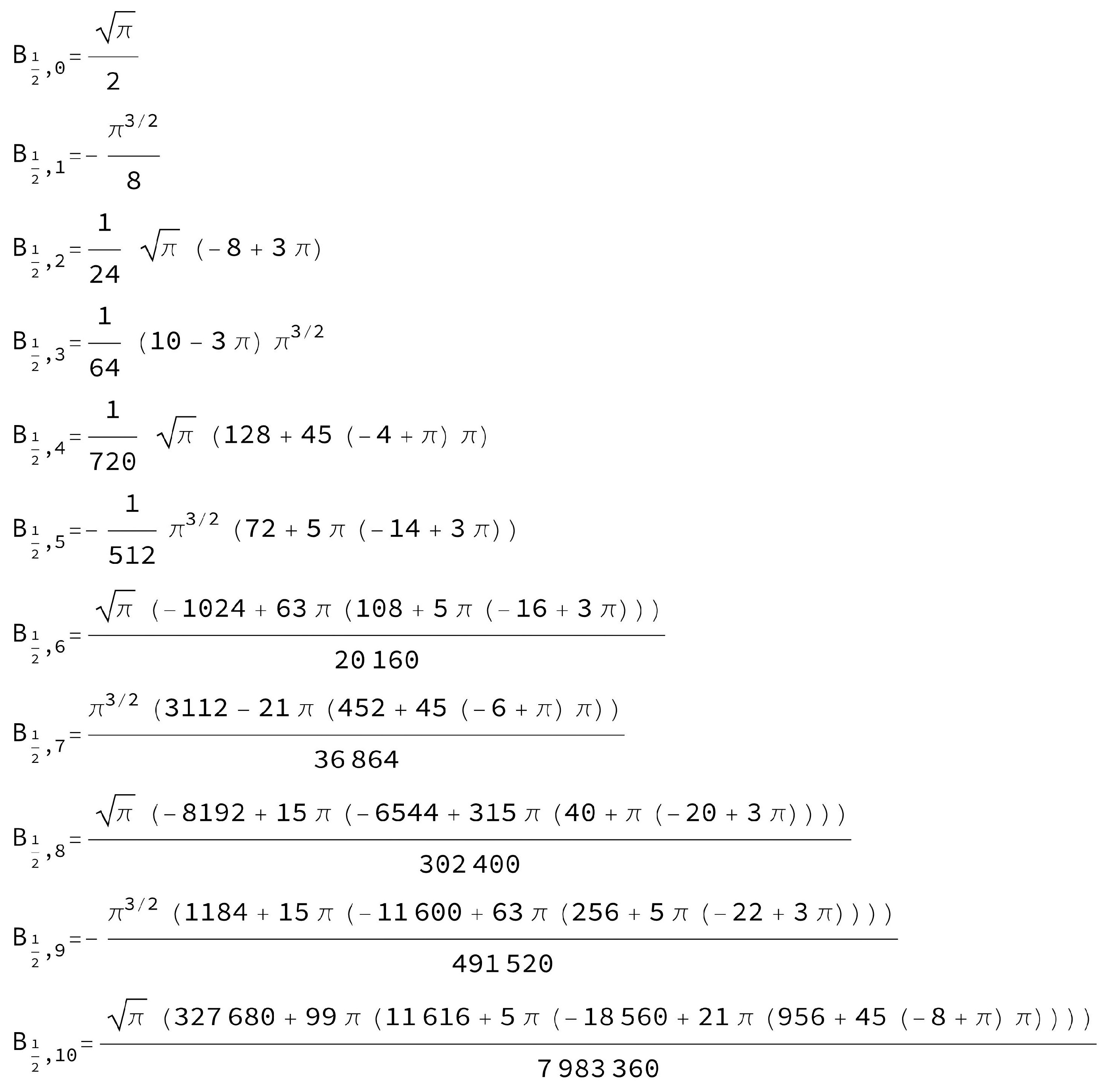
A more extended table is reported in Figure 1.

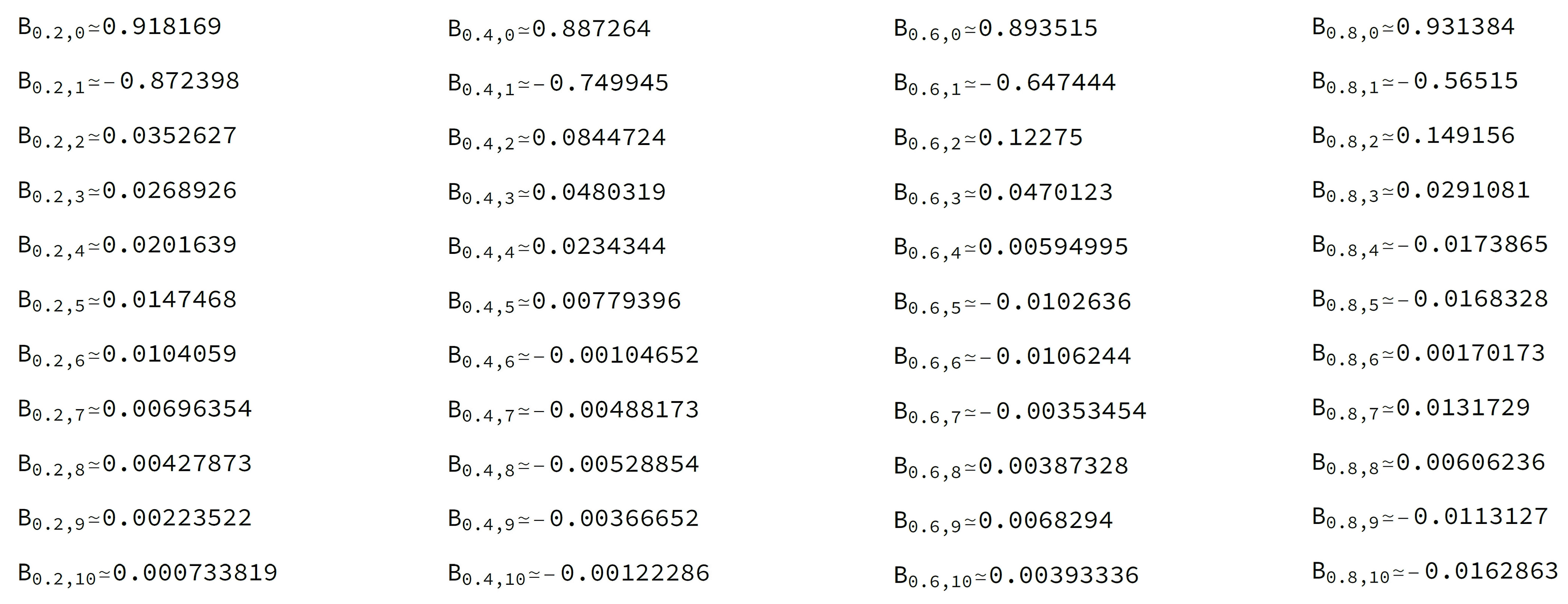
The Bernoulli numbers $B_{\alpha ,k}$ with fractional indices $\alpha =0.2,0.4,0.6,0.8$ for $0\le k\le 10$ are reported in Figure 2.

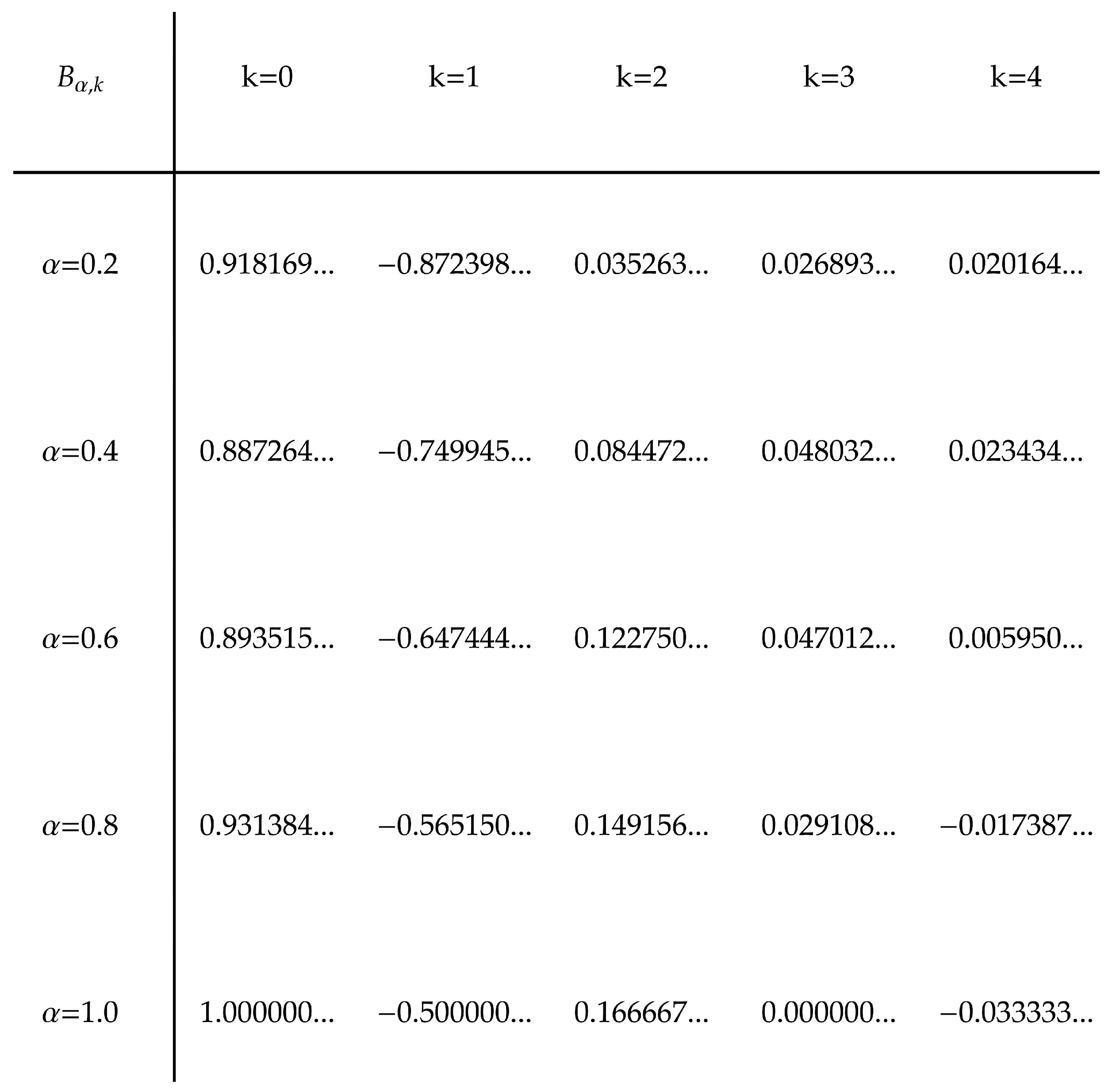
The convergence of the Bernoulli numbers $B_{\alpha ,k}$ to the classical $B_k$ is shown in the table contained in Figure 3.

3.3. Fractional Index Fractional Bernoulli Polynomials

Starting from (3), we find

$$\begin{array}{c}\hfill {\displaystyle \sum _{n=0}^{\infty }\frac{x^{(n+1)\alpha }{z}^{n\alpha }}{\Gamma (n\alpha +1)}=\sum _{k=1}^{\infty }\frac{x^{k\alpha }}{\Gamma (k\alpha +1)}\sum _{k=0}^{\infty }{B}_{\alpha ,k}\left(z\right)\frac{x^{k\alpha }}{\Gamma (k\alpha +1)},}\end{array}$$

$$\begin{array}{c}\hfill {\displaystyle \sum _{n=0}^{\infty }\frac{x^{(n+1)\alpha }{z}^{n\alpha }}{\Gamma (n\alpha +1)}=\sum _{k=0}^{\infty }\frac{x^{(k+1)\alpha }}{\Gamma \left(\right(k+1)\alpha +1)}\sum _{k=0}^{\infty }{B}_{\alpha ,k}\left(z\right)\frac{x^{k\alpha }}{\Gamma (k\alpha +1)},}\end{array}$$

$$\begin{array}{c}\hfill {\displaystyle \sum _{n=0}^{\infty }\frac{x^{(n+1)\alpha }{z}^{n\alpha }}{\Gamma (n\alpha +1)}=\sum _{n=0}^{\infty }\sum _{k=0}^n\frac{x^{(n+1)\alpha }{B}_{\alpha ,n-k}\left(z\right)}{\Gamma \left(\right(k+1)\alpha +1)\Gamma \left(\right(n-k)\alpha +1)},}\end{array}$$

so that, upon comparing coefficients of the same order, we obtain a triangular system. Therefore, we can state the following theorem:

Theorem 2. 

The fractional index fractional Bernoulli polynomials $B_{\alpha ,n}\left(z\right)$ can be sequentially constructed by solving the triangular system

$$\begin{array}{c}{B}_{\alpha ,0}\left(z\right)=\Gamma (\alpha +1),\hfill \\ {\displaystyle \sum _{k=0}^n\frac{B_{\alpha ,n-k}\left(z\right)\Gamma (n\alpha +1)}{\Gamma \left(\right(k+1)\alpha +1)\Gamma \left(\right(n-k)\alpha +1)}=z^{n\alpha },\forall n\ge 1,}\hfill \end{array}$$

(6)

The first few fractional index fractional Bernoulli polynomials are reported hereafter:

$$\begin{array}{c}{B}_{\alpha ,0}\left(z\right)=\Gamma (\alpha +1),\hfill \\ B_{\alpha ,1}\left(z\right)=\Gamma (\alpha +1)z^{\alpha }-\frac{\Gamma {(\alpha +1)}^3}{\Gamma (2\alpha +1)},\hfill \\ B_{\alpha ,2}\left(z\right)=\Gamma (\alpha +1)\left(\frac{\Gamma {(\alpha +1)}^2}{\Gamma (2\alpha +1)}-\frac{\Gamma (\alpha +1)\Gamma (2\alpha +1)}{\Gamma (3\alpha +1)}+\left(z^{\alpha }-1\right)z^{\alpha }\right),\hfill \\ B_{\alpha ,3}\left(z\right)=\Gamma (\alpha +1)\left(-\frac{\Gamma {(\alpha +1)}^3\Gamma (3\alpha +1)}{\Gamma {(2\alpha +1)}^3}+\frac{2\Gamma {(\alpha +1)}^2}{\Gamma (2\alpha +1)}\right.\hfill \\ \left.+\Gamma (\alpha +1)\Gamma (3\alpha +1)\left(-\frac{1}{\Gamma (4\alpha +1)}-\frac{\left(z^{\alpha }-1\right)z^{\alpha }}{\Gamma {(2\alpha +1)}^2}\right)+\left(z^{2\alpha }-1\right)z^{\alpha }\right),\hfill \\ B_{\alpha ,4}\left(z\right)=\Gamma (\alpha +1)\left(-\frac{3\Gamma {(\alpha +1)}^3\Gamma (4\alpha +1)}{\Gamma {(2\alpha +1)}^2\Gamma (3\alpha +1)}+\frac{\Gamma {(\alpha +1)}^4\Gamma (4\alpha +1)}{\Gamma {(2\alpha +1)}^4}\Gamma {(\alpha +1)}^2\left(\frac{\Gamma (4\alpha +1)}{\Gamma {(3\alpha +1)}^2}+\frac{2}{\Gamma (2\alpha +1)}+\frac{\Gamma (4\alpha +1)\left(z^{\alpha }-1\right)z^{\alpha }}{\Gamma {(2\alpha +1)}^3}\right)\right.\hfill \\ \left.+\left(z^{3\alpha }-1\right)z^{\alpha }+\Gamma (\alpha +1)\Gamma (4\alpha +1)\left(-\frac{1}{\Gamma (5\alpha +1)}-\frac{\left(z^{2\alpha }+z^{\alpha }-2\right)z^{\alpha }}{\Gamma (2\alpha +1)\Gamma (3\alpha +1)}\right)\right).\hfill \end{array}$$

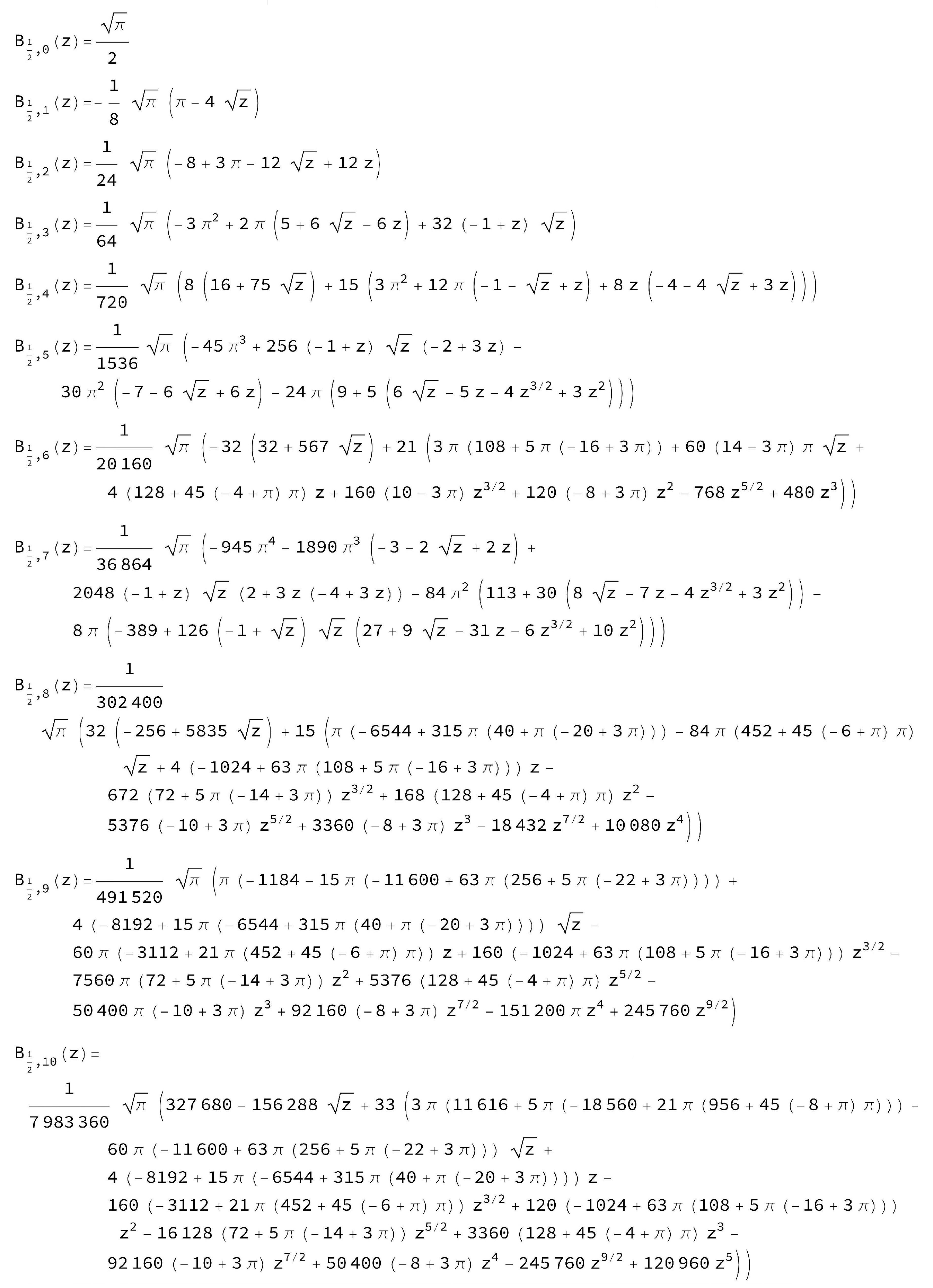
In the particular case when $\alpha =1/2$, we find the first ten fractional Bernoulli polynomials as reported in Figure 4.

Remark 2. 

Note that if $\alpha =1$, the fractional exponential ${\mathrm{Exp}}_{\alpha }\left(t\right)$ reduces to the ordinary exponential function $exp\left(t\right)$, and the fractional Bernoulli numbers and polynomials yield the ordinary classical ones.

4. Fractional Index Euler Numbers and Polynomials

We introduce the following definitions:

1.

For the fractional index Euler numbers $E_{\alpha ,k}$,

$$\begin{array}{c}\hfill {\displaystyle \frac{2{\mathrm{Exp}}_{\alpha }\left(x\right)}{{\mathrm{Exp}}_{\alpha }\left(2x\right)+1}=\sum _{k=0}^{\infty }{E}_{\alpha ,k}\frac{x^{k\alpha }}{\Gamma (k\alpha +1)},}\end{array}$$

(7)

2.

For the fractional index Euler polynomials $E_{\alpha ,k}\left(z\right)$,

$$\begin{array}{c}\hfill {\displaystyle \frac{2{\mathrm{Exp}}_{\alpha }\left(xz\right)}{{\mathrm{Exp}}_{\alpha }\left(2x\right)+1}=\sum _{k=0}^{\infty }{E}_{\alpha ,k}\left(z\right)\frac{x^{k\alpha }}{\Gamma (k\alpha +1)}.}\end{array}$$

(8)

4.1. Fractional Index Euler Numbers

We start from the fractional index Euler numbers exponential function (7) so that

$$\begin{array}{c}\hfill {\displaystyle 2{\mathrm{Exp}}_{\alpha }\left(x\right)=\left[{\mathrm{Exp}}_{\alpha }\left(2x\right)+1\right]\sum _{k=0}^{\infty }{E}_{\alpha ,k}\frac{x^{k\alpha }}{\Gamma (k\alpha +1)},}\end{array}$$

$$\begin{array}{c}\hfill {\displaystyle 2\sum _{n=0}^{\infty }\frac{x^{n\alpha }}{\Gamma (n\alpha +1)}=\sum _{k=0}^{\infty }\frac{E_{\alpha ,k}{x}^{k\alpha }}{\Gamma (k\alpha +1)}+\sum _{k=0}^{\infty }\frac{2^{k\alpha }{x}^{k\alpha }}{\Gamma (k\alpha +1)}\sum _{k=0}^{\infty }\frac{E_{\alpha ,k}{x}^{k\alpha }}{\Gamma (k\alpha +1)},}\end{array}$$

$$\begin{array}{c}\hfill {\displaystyle 2\sum _{n=0}^{\infty }\frac{x^{n\alpha }}{\Gamma (n\alpha +1)}=\sum _{n=0}^{\infty }\frac{E_{\alpha ,n}{x}^{n\alpha }}{\Gamma (n\alpha +1)}+\sum _{n=0}^{\infty }\sum _{k=0}^n\frac{2^{k\alpha }{E}_{\alpha ,n-k}{x}^{n\alpha }}{\Gamma (k\alpha +1)\Gamma \left(\right(n-k)\alpha +1)}.}\end{array}$$

(9)

Then, by equating coefficients of the same order, we obtain

$$\begin{array}{c}\hfill {\displaystyle \frac{2}{\Gamma (n\alpha +1)}=\frac{E_{\alpha ,n}}{\Gamma (n\alpha +1)}+\sum _{k=0}^n\frac{2^{k\alpha }{E}_{\alpha ,n-k}}{\Gamma (k\alpha +1)\Gamma \left(\right(n-k)\alpha +1)},}\end{array}$$

which results in a triangular system of algebraic equations. Therefore, we can state the following theorem:

Theorem 3. 

The Euler numbers with fractional indices $E_{\alpha ,k}$ can be sequentially computed by solving the triangular system

$$\begin{array}{c}\hfill \begin{array}{c}{E}_{\alpha ,0}=1,\hfill \\ {\displaystyle E_{\alpha ,n}+\sum _{k=0}^n\frac{2^{k\alpha }\Gamma (n\alpha +1)E_{\alpha ,n-k}}{\Gamma (k\alpha +1)\Gamma \left(\right(n-k)\alpha +1)}=2.}\hfill \end{array}\end{array}$$

(10)

We find, in particular,

$$\begin{array}{c}\hfill \begin{array}{c}{E}_{\alpha ,0}=1,\hfill \\ E_{\alpha ,1}=1-2^{\alpha -1},\hfill \\ {\displaystyle E_{\alpha ,2}=1-2^{2\alpha -1}+\frac{(2^{2\alpha -2}-2^{\alpha -1})\Gamma (2\alpha +1)}{{[\Gamma (\alpha +1)]}^2},}\hfill \end{array}\end{array}$$

and so on.

4.2. The Fractional Index Euler Numbers for $\alpha =1/2$

In this particular case where $\alpha =1/2$, the above system writes

$$\begin{array}{c}\hfill {\displaystyle E_{1/2,n}+\sum _{k=0}^n\frac{2^{k/2}\Gamma (n/2+1)E_{1/2,n-k}}{\Gamma (k/2+1)\Gamma \left(\right(n-k)/2+1)}-2=0,}\end{array}$$

The first few entries are

$$\begin{array}{c}\hfill \begin{array}{c}{E}_{1/2,0}=1\\ {\displaystyle E_{1/2,1/2}=1-\frac{1}{\sqrt{2}}\simeq 0.2928932\cdots }\\ {\displaystyle E_{1/2,1}=\frac{2-2\sqrt{2}}{\pi }\simeq -0.2636965\cdots }\end{array}\end{array}$$

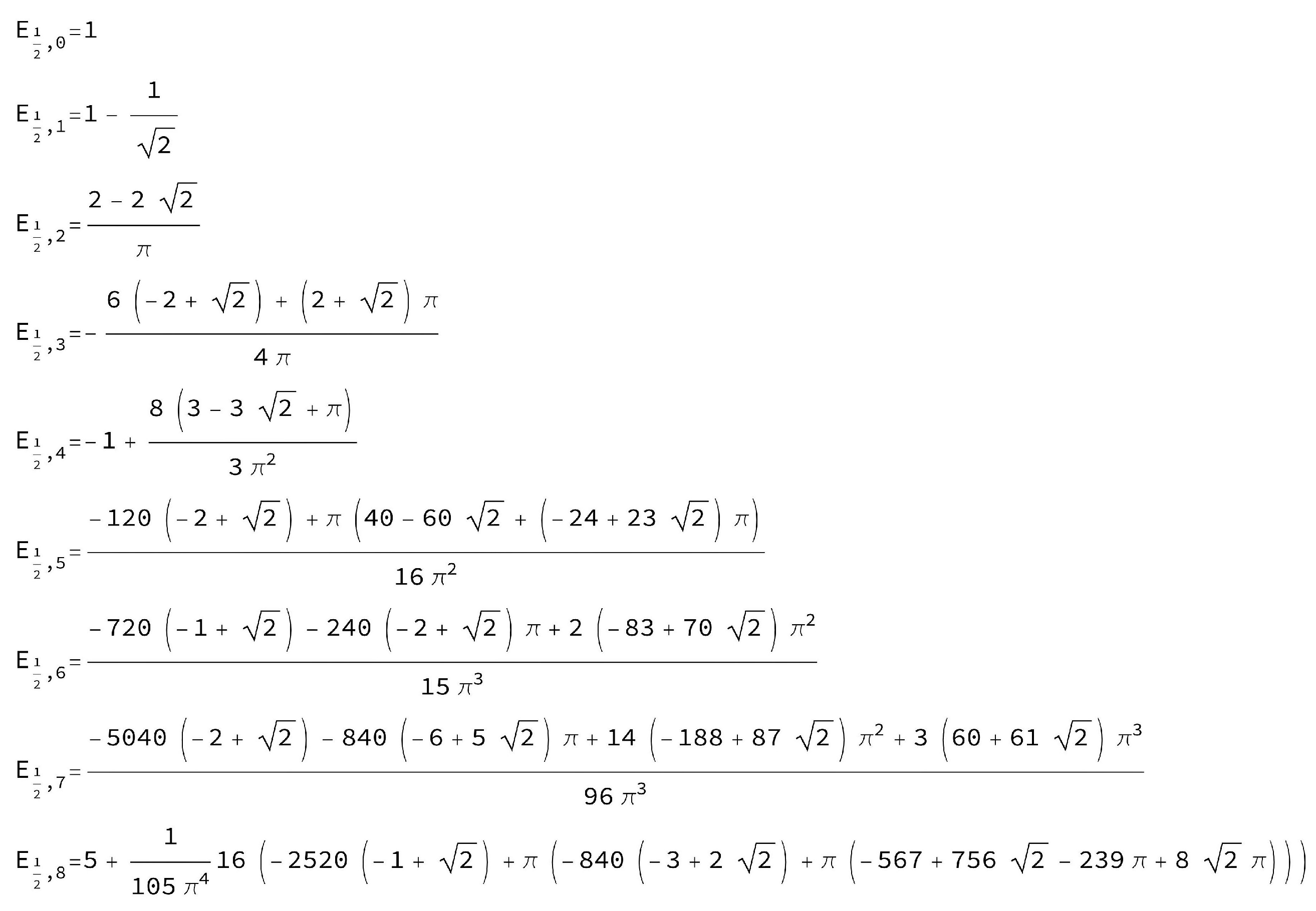
A more extended sequence is reported in Figure 5.

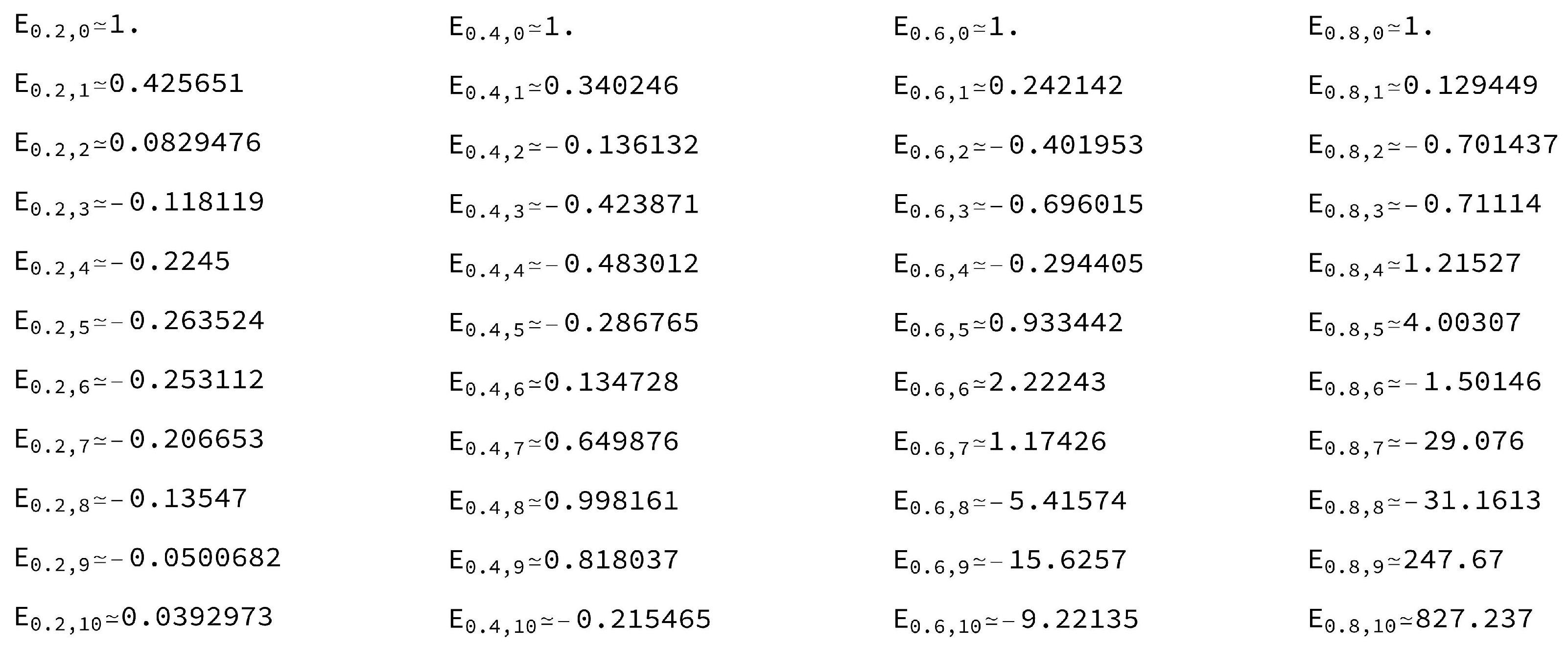
The Euler numbers $E_{\alpha ,k}$ with fractional indices for $\alpha =0.2,0.4,0.6,0.8$, and with $0\le k\le 10$, are shown in Figure 6.

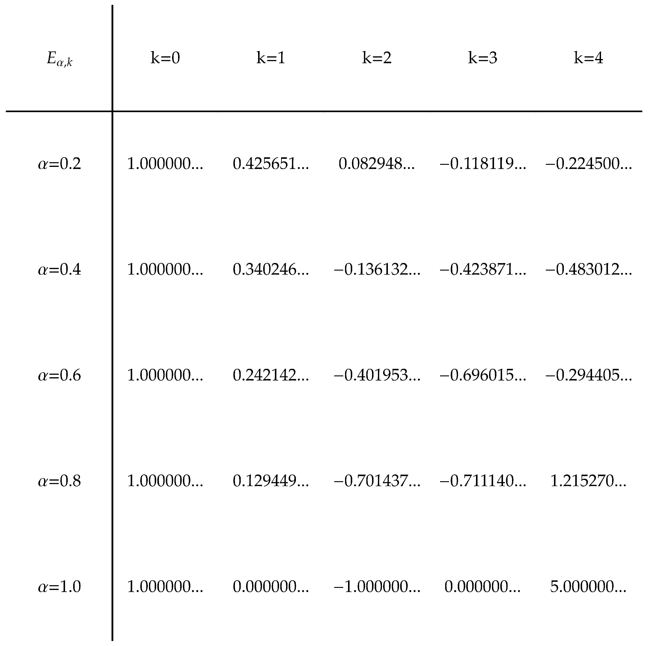
The convergence of the Euler numbers $E_{\alpha ,k}$ to the classical $E_k$ is shown in the table contained in Figure 7.

4.3. Fractional Index Fractional Euler Polynomials

Using the generating function in (8), we find

$$\begin{array}{c}\hfill {\displaystyle 2\sum _{n=0}^{\infty }\frac{x^{n\alpha }{z}^{n\alpha }}{\Gamma (n\alpha +1)}=\sum _{k=0}^{\infty }\frac{E_{\alpha ,k}\left(z\right)x^{k\alpha }}{\Gamma (k\alpha +1)}+\sum _{k=0}^{\infty }\frac{2^{k\alpha }{x}^{k\alpha }}{\Gamma (k\alpha +1)}\sum _{k=0}^{\infty }\frac{E_{\alpha ,k}\left(z\right)x^{k\alpha }}{\Gamma (k\alpha +1)},}\end{array}$$

$$\begin{array}{c}\hfill {\displaystyle 2\sum _{n=0}^{\infty }\frac{x^{n\alpha }{z}^{n\alpha }}{\Gamma (n\alpha +1)}=\sum _{n=0}^{\infty }\frac{E_{\alpha ,n}\left(z\right)x^{n\alpha }}{\Gamma (n\alpha +1)}+\sum _{n=0}^{\infty }\sum _{k=0}^n\frac{2^{(n-k)\alpha }{x}^{n\alpha }{E}_{\alpha ,k}\left(z\right)}{\Gamma \left(\right(n-k)\alpha +1)\Gamma (k\alpha +1)}.}\end{array}$$

Then, by equating coefficients of the same order, we find

$$\begin{array}{c}\hfill {\displaystyle \frac{2z^{n\alpha }}{\Gamma (n\alpha +1)}=\frac{E_{\alpha ,n}\left(z\right)}{\Gamma (n\alpha +1)}+\sum _{k=0}^n\frac{2^{(n-k)\alpha }{E}_{\alpha ,k}\left(z\right)}{\Gamma \left(\right(n-k)\alpha +1)\Gamma (k\alpha +1)},}\end{array}$$

(11)

which results in a triangular system of algebraic equations. Therefore, we can state the following theorem:

Theorem 4. 

The fractional index fractional Euler polynomials $E_{\alpha ,n}\left(z\right)$ can be sequentially constructed by solving the triangular system

$$\begin{array}{c}\hfill \begin{array}{c}{E}_{\alpha ,0}\left(z\right)=1,\hfill \\ {\displaystyle \frac{1}{2}\left[{\displaystyle E_{\alpha ,n}\left(z\right)+\sum _{k=0}^n\frac{2^{(n-k)\alpha }\Gamma (n\alpha +1)E_{\alpha ,k}\left(z\right)}{\Gamma \left(\right(n-k)\alpha +1)\Gamma (k\alpha +1)}}\right]=z^{n\alpha }.}\hfill \end{array}\end{array}$$

(12)

The first few fractional index fractional Euler polynomials are reported hereafter:

$$\begin{array}{c}\hfill \begin{array}{c}{E}_{\alpha ,0}\left(z\right)=1,\hfill \\ E_{\alpha ,1}\left(z\right)=z^{\alpha }-2^{\alpha -1},\hfill \\ E_{\alpha ,2}\left(z\right)=-2^{2\alpha -1}+z^{2\alpha }+\frac{2^{\alpha -2}\Gamma (2\alpha +1)\left(2^{\alpha }-2z^{\alpha }\right)}{\Gamma {(\alpha +1)}^2},\hfill \\ E_{\alpha ,3}\left(z\right)=-2^{3\alpha -1}+z^{3\alpha }+\frac{2^{\alpha -3}\Gamma (3\alpha +1)\left(\frac{4\Gamma {(\alpha +1)}^2\left(4^{\alpha }-z^{\alpha }\left(2^{\alpha }+z^{\alpha }\right)\right)}{\Gamma (2\alpha +1)}-2^{\alpha }\left(2^{\alpha }-2z^{\alpha }\right)\right)}{\Gamma {(\alpha +1)}^3},\hfill \\ E_{\alpha ,4}\left(z\right)=-2^{4\alpha -1}+z^{4\alpha }+2^{\alpha -4}\Gamma (4\alpha +1)\left(\frac{2^{\alpha +2}\left(4^{\alpha }-2z^{2\alpha }\right)}{\Gamma {(2\alpha +1)}^2}+\frac{4^{\alpha }\left(2^{\alpha }-2z^{\alpha }\right)}{\Gamma {(\alpha +1)}^4}+\frac{2^{\alpha +1}\left(2z^{\alpha }\left(2^{\alpha +1}+z^{\alpha }\right)-34^{\alpha }\right)}{\Gamma {(\alpha +1)}^2\Gamma (2\alpha +1)}\right.\hfill \\ \left.+\frac{8\left(8^{\alpha }-z^{\alpha }\left(4^{\alpha }+z^{2\alpha }\right)\right)}{\Gamma (\alpha +1)\Gamma (3\alpha +1)}\right).\hfill \end{array}\end{array}$$

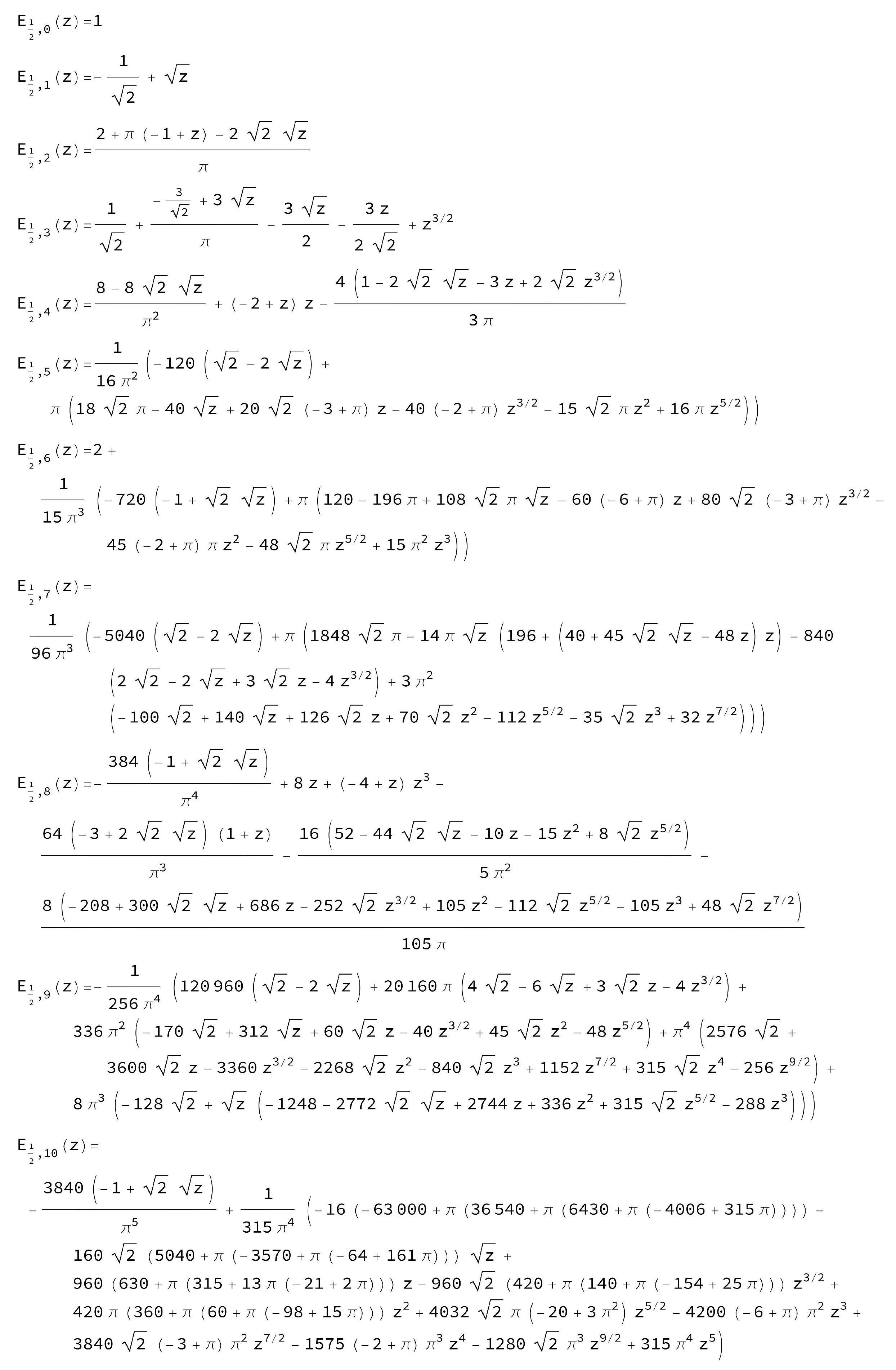
In the particular case when $\alpha =1/2$, we find the first ten fractional Euler polynomials, which are reported in Figure 8.

Remark 3. 

Note that if $\alpha =1$, the fractional exponential ${\mathrm{Exp}}_{\alpha }\left(t\right)$ reduces to the ordinary exponential function $exp\left(t\right)$, and the fractional Euler numbers and polynomials yield the ordinary classical ones.

5. Conclusions

We have demonstrated the use of the fractional exponential, which was recently investigated in [13], to create fractional-index-based versions of the traditional Bernoulli and Euler numbers, as well as fractional Bernoulli and Euler polynomials.

With the assistance of the computer algebra system Mathematica, we have derived several tables featuring these new special numbers and fractional polynomials for certain values of the parameter $\alpha$ between 0 and 1. We have highlighted the case where $\alpha$ equals 1/2. The relevant tables demonstrate how these entities converge to the classical numbers as $\alpha$ approaches 1. We have limited ourselves to simpler cases for the sake of brevity, but many further extensions are possible.

In forthcoming articles, we will show properties of the classical numbers and polynomials that still remain valid for the fractional counterparts introduced in this research study.

References

- Samko, S.; Kilbas, A.A.; Marichev, O. Fractional Integrals and Derivatives; Taylor & Francis: Oxfordshire, UK, 1993. [Google Scholar]
- Kilbas, A.A.; Srivastava, H.M.; Trujillo, J.J. Theory and Applications of Fractional Differential Equations. In North-Holland Mathematics Studies; Elsevier: Amsterdam, The Netherlands, 2006; Volume 204. [Google Scholar]
- Gorenflo, F.; Mainardi, F. Fractional Calculus: Integral and Differential Equations of Fractional Order. In Fractals and Fractional Calculus in Continuum Mechanics; Carpinteri, A., Mainardi, F., Eds.; Springer: New York, NY, USA, 1997; pp. 223–276. [Google Scholar]
- Mainardi, F.; Luchko, Y.; Pagnini, G. The fundamental solution of the space-time fractional diffusion equation. Fract. Calc. Appl. Anal. 2001, 4, 153–192. [Google Scholar]
- Groza, G.; Jianu, M. Functions represented into fractional Taylor series. In Proceedings of the 1st International Conference on Computational Methods and Applications in Engineering (ICCMAE 2018), Timisoara, Romania, 23–26 May 2018; Volume 29, p. 01017. [Google Scholar] [CrossRef]
- Caratelli, D.; Natalini, P.; Ricci, P.E. Examples of expansions in fractional powers and applications. Symmetry 2023, 15, 1702. [Google Scholar] [CrossRef]
- Ortigueira, M.D.; Trujillo, J.J.; Martynyuk, V.I.; Coito, F.J.V. A generalized power series and its application in the inversion of transfer functions. Signal Process. 2015, 107, 238–245. [Google Scholar] [CrossRef]
- Ortigueira, M.D. A New Look at the Initial Condition Problem. Mathematics 2022, 10, 1771. [Google Scholar] [CrossRef]
- Ortigueira, M.D.; Bengocheab, G. A new look at the fractionalization of the logistic equation. Phys. A 2017, 467, 554–561. [Google Scholar] [CrossRef]
- Beghin, L.; Caputo, M. Commutative and associative properties of the Caputo fractional derivative and its generalizing convolution operator. Commun. Nonlinear Sci. Numer. Simul. 2020, 89, 105338. [Google Scholar] [CrossRef]
- Woldeyohannes, E. Fractional Bernoulli Numbers and Polynomials. Ph.D. Thesis, Addis Ababa University, Addis Ababa, Ethiopia, 2019. [Google Scholar]
- Leinartas, E.K.; Shishkina, O.A. The discrete analog of the Newton-Leibniz formula in the problem of summation over simple lattice points. J. Sib. Fed. Univ. Math. Phys. 2019, 12, 503–508. [Google Scholar] [CrossRef]
- Caratelli, D.; Ricci, P.E. An Introduction to Fractional Exponential Functions and Applications. 2023; submitted. [Google Scholar]
- Caratelli, D.; Ricci, P.E. Fractional Hermite-Kampé de Fériet and Related Polynomials. 2023; submitted. [Google Scholar]
- Mishra, A.; Birla Institute of Technology & Science, Pilani Pilani Campus, Vidya Vihar, Rajasthan Pilani, India. Special Integrals. Personal communication, 2023.
- Araci, S.; Sen, E.; Acikgoz, M.; Orucoglu, K. Identities Involving Some New Special Polynomials Arising from the Applications of Fractional Calculus. Appl. Math. Inf. Sci. 2015, 9, 2657–2662. [Google Scholar]
- Bretti, G.; Ricci, P.E. Laguerre-type Special functions and population dynamics. Appl. Math. Comp. 2007, 187, 89–100. [Google Scholar] [CrossRef]
- Ricci, P.E.; Tavkhelidze, I. An introduction to operational techniques and special polynomials. J. Math. Sci. 2009, 157, 161–189. Translated from: Contemporary Mathematics and its Applications—(Sovremennaya Matematika i ee Prilozheniya); vol. 51, (in Russian), ISSN: 1512-1712. [Google Scholar] [CrossRef]
Figure 1.
Sequence of the Bernoulli numbers for .
Figure 2.
Sequence of the Bernoulli numbers with fractional indices for .
Figure 3.
Convergence of the fractional index Bernoulli numbers to the classical ones .
Figure 4.
Sequence of the fractional Bernoulli polynomials for .
Figure 5.
Sequence of the Euler numbers for .
Figure 6.
Sequence of the Euler numbers with fractional indices for .
Figure 7.
Convergence of the fractional index Euler numbers to the classical ones .
Figure 8.
Sequence of the fractional Euler polynomials for .
Disclaimer/Publisher’s Note: The statements, opinions and data contained in all publications are solely those of the individual author(s) and contributor(s) and not of MDPI and/or the editor(s). MDPI and/or the editor(s) disclaim responsibility for any injury to people or property resulting from any ideas, methods, instructions or products referred to in the content. |
© 2023 by the authors. Licensee MDPI, Basel, Switzerland. This article is an open access article distributed under the terms and conditions of the Creative Commons Attribution (CC BY) license (https://creativecommons.org/licenses/by/4.0/).
Share and Cite
MDPI and ACS Style
Caratelli, D.; Natalini, P.; Ricci, P.E. Fractional Bernoulli and Euler Numbers and Related Fractional Polynomials—A Symmetry in Number Theory. Symmetry 2023, 15, 1900. https://doi.org/10.3390/sym15101900
AMA Style
Caratelli D, Natalini P, Ricci PE. Fractional Bernoulli and Euler Numbers and Related Fractional Polynomials—A Symmetry in Number Theory. Symmetry. 2023; 15(10):1900. https://doi.org/10.3390/sym15101900
Chicago/Turabian StyleCaratelli, Diego, Pierpaolo Natalini, and Paolo Emilio Ricci. 2023. "Fractional Bernoulli and Euler Numbers and Related Fractional Polynomials—A Symmetry in Number Theory" Symmetry 15, no. 10: 1900. https://doi.org/10.3390/sym15101900
Note that from the first issue of 2016, this journal uses article numbers instead of page numbers. See further details here.