
Examples of Expansions in Fractional Powers, and Applications

1
The Antenna Company, High Tech Campus 41, 5656 AE Eindhoven, The Netherlands
2
Department of Electrical Engineering, Eindhoven University of Technology, P.O. Box 513, 5600 MB Eindhoven, The Netherlands
3
Department of Mathematics and Physics, Roma Tre University, Largo San Leonardo Murialdo, 1, 00146 Rome, Italy
4
Mathematics Section, International Telematic University UniNettuno, Corso Vittorio Emanuele II, 39, 00186 Rome, Italy
*
Author to whom correspondence should be addressed.
Symmetry 2023, 15(9), 1702; https://doi.org/10.3390/sym15091702
Submission received: 19 July 2023
/
Revised: 25 August 2023
/
Accepted: 2 September 2023
/
Published: 6 September 2023
(This article belongs to the Special Issue Special Functions, Integral Transforms and Polynomial Sequences in Real World with Symmetry)
Abstract
:We approximate the solution of a generalized form of the Bagley–Torvik equation using Taylor’s expansions in fractional powers. Then, we study the fractional Laguerre-type logistic equation by considering the fractional exponential function and its Laguerre-type form. To verify our findings, we conduct numerical tests using the computer algebra program Mathematica.
Keywords:
fractional differential equations; Bagley–Torvik equation; generalized exponential function; Mittag–Leffler function; fractional Laguerre-type logistic equationMSC:
34A08; 26A33; 34A251. Introduction
In a recent article [1], we used expansions in fractional powers to solve, in an elementary way, several multi-term fractional differential equations, which appeared in the literature (see, e.g., [2,3,4,5,6,7,8,9]). The fractional derivative is a critical concept for innumerable applications in the most diverse fields of applied sciences. Several definitions are examined and compared in classic papers (see e.g., [10,11,12]), where fractional differential equations [13] are also studied.
Without going into this vast field of investigation, in the article above [1], we limited ourselves to considering the Euler’s definition for the fractional derivative that falls within the one given by Caputo [14], and we only considered expansions in fractional power series. The powers considered in our expansions enjoy a symmetrical property, being integer multiples of a given number
This method has been analyzed in the work of Groza–Jianu [15], where the main results valid for ordinary power series expansions were extended to the case of fractional power exponents.
In this article, in Section 2, we extend the results obtained in [1] by studying a generalization of the classical Bagley–Torvik equation [16].
Moreover, in Section 3, we introduce the fractional version of the exponential function, which is related to the Mittag–Leffler function [17], frequently used in the framework of studies concerning fractional derivative theory and applications.
As is well known, the exponential function is the basic tool for constructing special functions and polynomials, often through suitable generating functions, which gave rise to symmetric or antisymmetric functions. Extending this function to the fractional case makes the generalization of many classical polynomial sets and functional operators possible.
This is the aim of our investigation involving the study of fractional versions of many mathematical special functions, special polynomials and numbers.
Our goal is to show how these generalized entities, depending on a parameter (with ), approach their corresponding classical counterparts as approaches 1. In this way, one can develop fractional versions of classical differential equations, including those related to population dynamics, and define fractional Laplace transforms, as well as fractional special numbers. Related articles are currently being published on these topics.
In Section 4, we recall the fractional-order logistic equation already examined in a preceding article, with the purpose of generalizing that to the Laguerre-type case.
The Laguerre-type exponentials and derivatives are recalled in Section 5 and are extended to the fractional case.
It is worth noting that the Laguerre derivative and the associated Laguerre-type special functions [18,19] determine a symmetry in the space of analytic functions. In fact, the operator introduces a linear differential isomorphism, acting on the space of analytic functions of the x variable. By using this isomorphism, a parallel structure is created within this space, so that the differentiation properties can be immediately derived.
Furthermore, iterations of the Laguerre derivative can be defined, and this parallelism can be iterated too, in an endless way. Therefore, a cyclic construction is created within the space that repeats the same structure at a higher level of differentiation order. It is one of the great cycles that sometimes occur within mathematical theories.
2. The Bagley–Torvik Equation
In 1984, Torvik and Bagley [16] first proposed a fractional order differential equation to model the viscoelastic behavior of geological strata, as well as metals, and glasses. They showed the effectiveness of their approach in describing structures containing elastic and viscoelastic components. The so called Bagley–Torvik equation became a model to test the solution of fractional differential equations, with suitable initial conditions.
We consider the following inhomogeneous Bagley–Torvik-type fractional differential equation (see [15]), with special initial conditions
Put
Since
and in Equation (1) the derivatives of order and 2 appear, we put in the expansion (3). As , we have
and
Substituting into Equation (1), we find
Equating the coefficients of equal t-powers, we find a triangular system, which recursively gives the coefficients of the solution (3).
2.1. Convergence Results
Let A and B be positive numbers, and suppose the sequence is bounded, i.e., .
We have put, for example, , , and we have found that the coefficients alternate in sign and tend to zero as .
We first prove that the coefficients of the series (3) are in the order of the reciprocal of the Gamma function of , so that the series is absolutely convergent in the whole complex plane. Then, we show that, on the real axis, the Nth remainder term tends to zero when .
Consequently,
assuming , and consequently, , with , we have
so that
and
Then, we find
so that the series is absolutely convergent in the whole complex plane, as its convergence radius is .
Furthermore, according to the Leibniz theorem, on the positive real axis, the alternating series is convergent and the remainder term resulting from the truncation of the series at the index N is bounded by the first neglected term, that is
2.2. Numerical Results
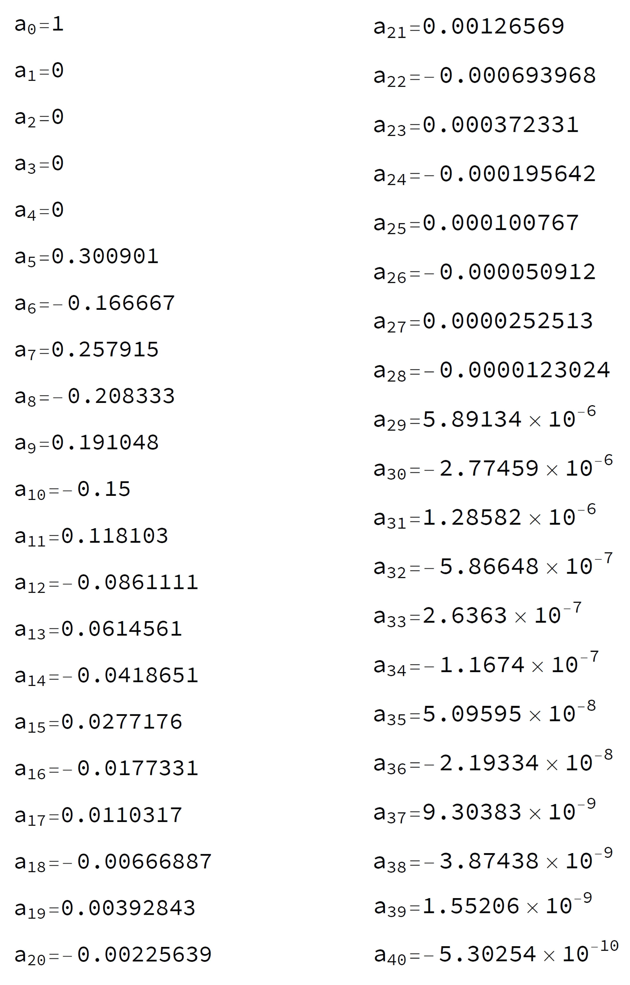
Assuming , , and using the above recursion, we find the following the Table of the coefficients , reported in Figure 1.
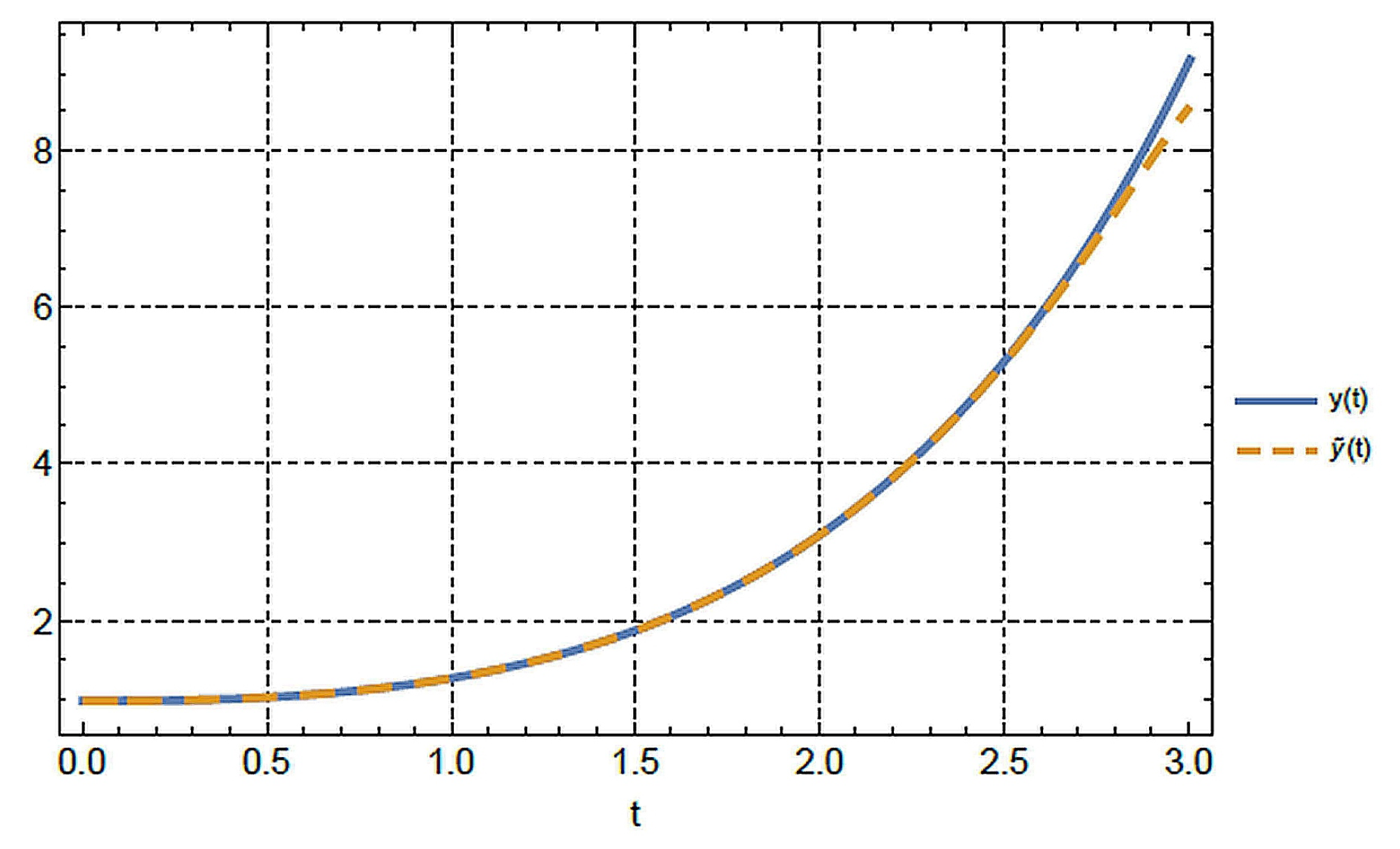
The graph of the approximate solution is depicted in Figure 2.
3. The Fractional Exponentials
Note that in the particular case , the second member of the classical Bagley–Torvik equation is an extension of the exponential function:
It is convergent in the whole complex plane, as the same holds for the classical exponential .
Furthermore, according to the fractional differentiation rule of powers, the following results
In general, putting
we find
Remark 1.
Recalling the Mittag–Leffler function [17]
assuming , and substituting x with results in
so that the fractional exponentials can be reduced to the Mittag–Leffler function.
In particular, we have:
4. The Fractional-Order Logistic Equation
We consider the fractional-order logistic initial value problem [21]
In a recent paper [20], we proved the result
Theorem 1.
Setting
the solution of the fractional-order logistic initial value problem in Equation (8) is obtained by computing the coefficients through the following recursion
Example
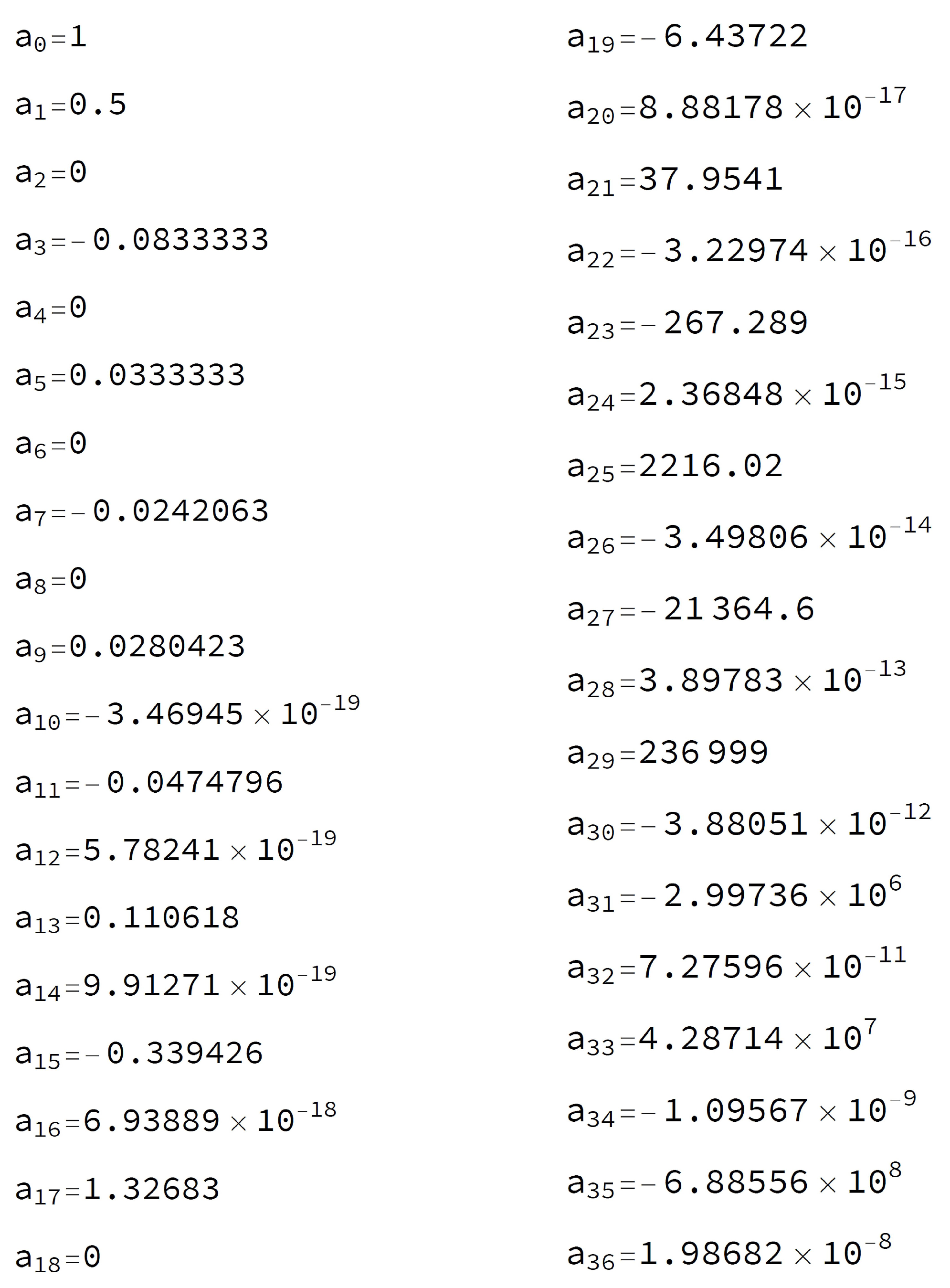
Assuming , and putting , we find the following Table for the coefficients, , reported in Figure 3.
5. The Laguerre-Type Exponentials
In preceding articles [18,19], the Laguerre-type exponential
has been introduced in connection with the Laguerre-type derivative
Namely, it is an eigenfunction of this operator, since (complex constant), resulting in the following equation:
In general, for any integer , the higher-order Laguerre-type exponentials
satisfy the eigenvalue property concerning the nth order Laguerre derivative
where denote the Stirling numbers of the second kind, since
The Laguerre-type special functions have been considered in preceding papers, and the relevant properties have been examined. It turned out that the properties of Laguerre-type special functions exhibit symmetric properties with respect to those of the corresponding ordinary ones. This is a consequence of a differential isomorphism in the space of analytic functions that connects ordinary and Laguerre-type special functions. Such isomorphism is described in [19].
5.1. The Fractional Laguerre-Exponentials
Introducing the fractional Laguerre-type exponential of order ,
we found that
More generally, putting
and considering the iterated Laguerre-type operator, which embeds fractional derivatives, results in the following equation:
Of course, the results of this section, and the relevant application, could be generalized to any value of , ; but, for the sake of conciseness, we limit ourselves to the particular case because the technique used is always the same.
5.2. The Laguerre-Type Fractional-Order Logistic Equation
We consider the Laguerre-type fractional-order logistic initial value problem
We prove the following result:
Theorem 2.
Setting
the solution of the considered Laguerre-type fractional-order logistic initial value problem is obtained computing the coefficients using the recursion
Proof.
Using the fractional differentiation, we find
Substituting into the equation, we find
so that the recursion for the coefficients follows. □
5.3. Numerical Results
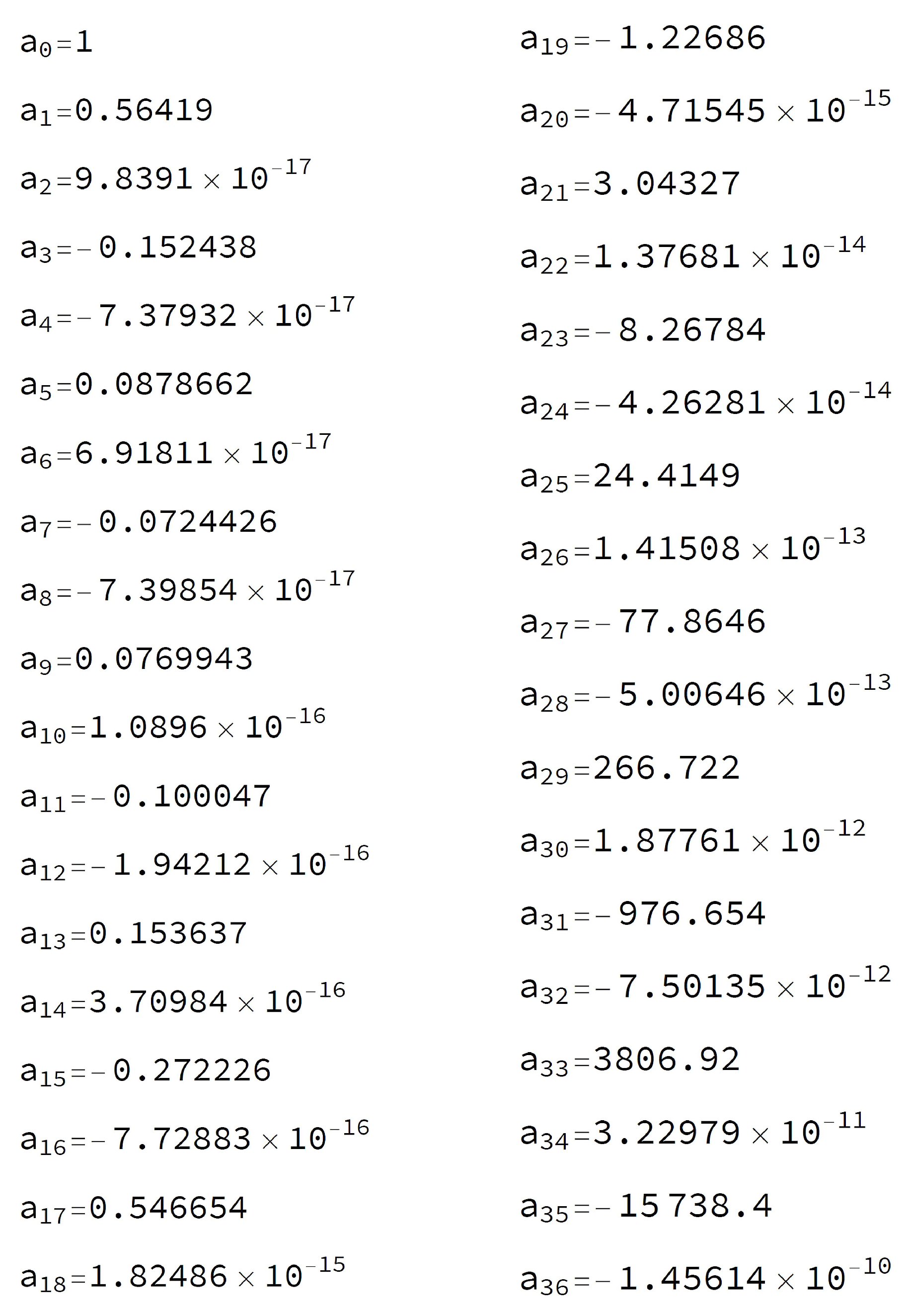
Assuming , , , and using the above recursion, we find the following Table of the coefficients , reported in Figure 4.
Remark 2.
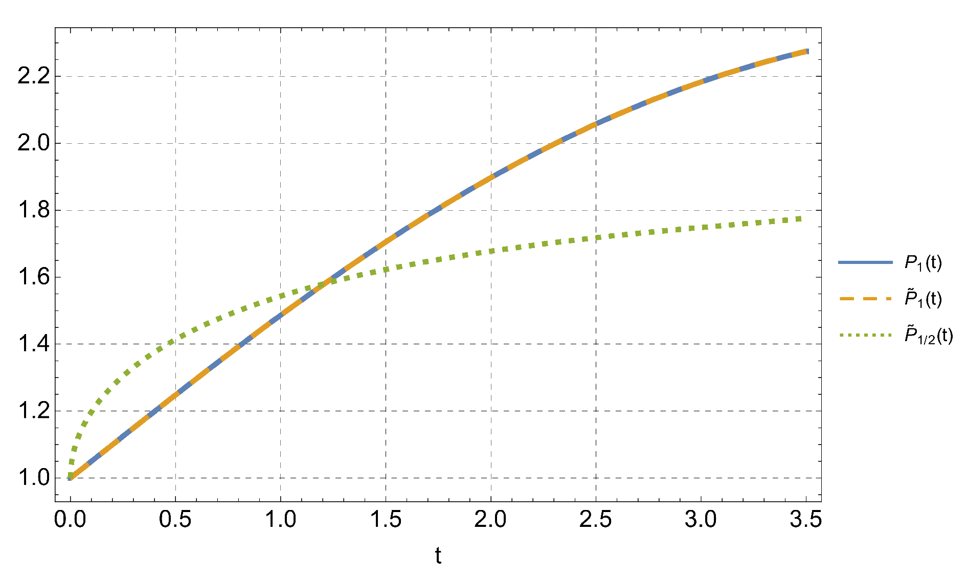
Note that in the Table contained in Figure 3, as well as in that in Figure 4, the values of the coefficients , with even index greater than 0, that is for , con, m a strictly positive integer, vanish or are so small that they cannot have any influence on the solution. The graph of the solution of problem 15, with a = 1/2, is shown in Figure 5.
![Symmetry 15 01702 g003]()
![Symmetry 15 01702 g004]()
Figure 3.
The coefficients of the solution (9), for the considered parameters, and .
Figure 3.
The coefficients of the solution (9), for the considered parameters, and .

Figure 4.
The coefficients for the Laguerre-type fractional logistic equation, with .

6. Conclusions
We have presented various findings within the context of fractional derivatives. Additionally, we have introduced a fractional version of the exponential function, which is connected to the Mittag–Leffler function that is commonly found in papers on fractional derivatives. In terms of the fractional derivative, this function shares the same eigenvalue characteristic as the traditional exponential has with respect to the ordinary derivative. As a result, many of the properties associated with analytic functions involving the exponential can be extended to fractional power series.
We are currently working on further articles that will delve deeper into this subject.
Author Contributions
Methodology, P.E.R.; software, D.C.; validation, D.C.; formal analysis, P.E.R. and P.N.; investigation, D.C.; data curation, D.C.; writing—original draft preparation, P.E.R.; writing—review and editing, D.C.; visualization, D.C. All authors have read and agreed to the published version of the manuscript.
Funding
This research received no external funding.
Data Availability Statement
Not applicable.
Conflicts of Interest
The authors declare no conflict of interest.
References
- Caratelli, D.; Natalini, P.; Ricci, P.E. Fractional differential equations and expansions in fractional powers. 2023; submitted. [Google Scholar]
- Abd-Elhameed, W.M.; Alsuyuti, M.M. Numerical Treatment of Multi-Term Fractional Differential Equations via a New Kind of Generalized Chebyshev Polynomials. Fractal Fract. 2023, 7, 74. [Google Scholar] [CrossRef]
- Ford, N.J.; Connolly, J.A. Systems-based decomposition schemes for the approximate solution of multi-term fractional differential equations. J. Comput. Appl. Math. 2009, 229, 382–391. [Google Scholar] [CrossRef]
- Ghoreishi, F.; Yazdani, S. An extension of the spectral Tau method for numerical solution of multi-order fractional differential equations with convergence analysis. Comput. Math. Appl. 2011, 61, 30–43. [Google Scholar] [CrossRef]
- Jafari, S.D.H.; Tajadodi, H. Solving a multi-order fractional differential equation using homotopy analysis method. J. King Saud Univ. Sci. 2011, 23, 151–155. [Google Scholar] [CrossRef]
- Seifollahi, M.; Shamloo, A. Numerical solution of nonlinear multi-order fractional differential equations by operational matrix of Chebyshev polynomials. World Appl. Program. 2013, 3, 85–92. [Google Scholar] [CrossRef]
- Talaei, Y.; Asgari, M. An operational matrix based on Chelyshkov polynomials for solving multi-order fractional differential equations. Neural Comput. Appl. 2018, 30, 1369–1376. [Google Scholar] [CrossRef]
- Bonab, Z.F.; Javidi, M. Higher order methods for fractional differential equation based on fractional backward differentiation formula of order three. Math. Comput. Simul. 2020, 172, 71–89. [Google Scholar] [CrossRef]
- Hesameddini, E.; Rahimi, A.; Asadollahifard, E. On the convergence of a new reliable algorithm for solving multi-order fractional differential equations. Commun. Nonlinear Sci. Numer. Simul. 2016, 34, 154–164. [Google Scholar] [CrossRef]
- Samko, S.; Kilbas, A.A.; Marichev, O. Fractional Integrals and Derivatives; Taylor & Francis: Abingdon, UK, 1993. [Google Scholar]
- Gorenflo, F.; Mainardi, F. Fractional Calculus: Integral and Differential Equations of Fractional Order. In Fractals and Fractional Calculus in Continuum Mechanics; Carpinteri, A., Mainardi, F., Eds.; Springer: New York, NY, USA, 1997; pp. 223–276. [Google Scholar]
- Mainardi, F.; Luchko, Y.; Pagnini, G. The fundamental solution of the space-time fractional diffusion equation. Fract. Calc. Appl. Anal. 2001, 4, 153–192. [Google Scholar]
- Kilbas, A.A.; Srivastava, H.M.; Trujillo, J.J. Theory and Applications of Fractional Differential Equations; North-Holland Mathematics Studies; Elsevier: Amsterdam, The Netherlands, 2006; Volume 204. [Google Scholar]
- Beghin, L.; Caputo, M. Commutative and associative properties of the Caputo fractional derivative and its generalizing convolution operator. Commun. Nonlinear Sci. Numer. Simul. 2020, 89, 105338. [Google Scholar] [CrossRef]
- Groza, G.; Jianu, M. Functions represented into fractional Taylor series. ITM Web Conf. 2019, 29, 01017. [Google Scholar] [CrossRef]
- Torvik, P.J.; Bagley, R.L. On the appearance of the fractional derivative in the behavior of real materials. J. Appl. Mech. 1984, 51, 294–298. [Google Scholar] [CrossRef]
- Gorflenko, R.; Kilbas, A.A.; Mainardi, F.; Rogosin, S.V. Mittag-Leffler Functions, Related Topics and Applications; Springer: New York, NY, USA, 2014. [Google Scholar]
- Bretti, G.; Ricci, P.E. Laguerre-type Special functions and population dynamics. Appl. Math. Comp. 2007, 187, 89–100. [Google Scholar] [CrossRef]
- Ricci, P.E.; Tavkhelidze, I. An introduction to operational techniques and special polynomials. J. Math. Sci. 2009, 157, 161–189. (In Russian) [Google Scholar] [CrossRef]
- Caratelli Ricci, P.E. A note on fractional-type models of population dynamics. 2023; submitted. [Google Scholar]
- El-Sayed, A.M.A.; El-Mesiry, A.E.M.; El-Saka, H.A.A. On the fractional-order logistic equation. Appl. Math. Lett. 2007, 20, 817–823. [Google Scholar] [CrossRef]
- Diethelm, K.; Ford, N.J.; Freed, A.D. A Predictor-Corrector Approach for the Numerical Solution of Fractional Differential Equations. Nonlinear Dyn. 2002, 29, 3–22. [Google Scholar] [CrossRef]
Figure 1.
The coefficients for .

Figure 2.
Graph of the solution using the coefficients vs. , obtained using the predictor–corrector method.
Figure 2.
Graph of the solution using the coefficients vs. , obtained using the predictor–corrector method.

Figure 5.
Graph of the solution of the problem (15) , using the coefficients of the Table in Figure 4 (dotted line), compared with the solutions of the Laguerre-type logistic equation using a predictor-corrector method (blue line) and a recursion method for approximating the coefficients (orange dashed line).

Disclaimer/Publisher’s Note: The statements, opinions and data contained in all publications are solely those of the individual author(s) and contributor(s) and not of MDPI and/or the editor(s). MDPI and/or the editor(s) disclaim responsibility for any injury to people or property resulting from any ideas, methods, instructions or products referred to in the content. |
© 2023 by the authors. Licensee MDPI, Basel, Switzerland. This article is an open access article distributed under the terms and conditions of the Creative Commons Attribution (CC BY) license (https://creativecommons.org/licenses/by/4.0/).
Share and Cite
MDPI and ACS Style
Caratelli, D.; Natalini, P.; Ricci, P.E. Examples of Expansions in Fractional Powers, and Applications. Symmetry 2023, 15, 1702. https://doi.org/10.3390/sym15091702
AMA Style
Caratelli D, Natalini P, Ricci PE. Examples of Expansions in Fractional Powers, and Applications. Symmetry. 2023; 15(9):1702. https://doi.org/10.3390/sym15091702
Chicago/Turabian StyleCaratelli, Diego, Pierpaolo Natalini, and Paolo Emilio Ricci. 2023. "Examples of Expansions in Fractional Powers, and Applications" Symmetry 15, no. 9: 1702. https://doi.org/10.3390/sym15091702
Note that from the first issue of 2016, this journal uses article numbers instead of page numbers. See further details here.