A Note on Varying G and Λ in Chern–Simons Modified Gravity

Abstract

We have considered the holographic dark energy and modified holographic Ricci dark energy models to analyze the time-dependent gravitational constant $G\left(t\right)$ and cosmological constant $\Lambda \left(t\right)$ in the context of Chern–Simons modified gravity theory. The FRW metric is used to examine the physical and kinematical properties of these models, which predicted the accelerated expansion phase of universe. Further, the $\Lambda \left(t\right)$ showed increasing trends while $G\left(t\right)$ showed decreasing trends for both cases. Finally, the range $-1.99\times {10}^{-10}{\mathrm{yr}}^{-1}\le \frac{\dot{G}}{G}\le 0$ was estimated mathematically, which is similar to the results obtained from observational data.

1. Introduction

Various theories of gravity have risen in popularity in the past few decades, due to recent cosmological observations [1,2]. To understand the concepts of late-time accelerated expansion of the universe and orientation curvatures of celestial objects in clusters within the general relativity (GR) framework, it is absolutely essential to postulate the origin of unidentified matter. Energy sources which fill the known universe and are supposed to influence gravity dynamics at cosmological levels are named dark energy (DE) and dark matter (DM). The challenge of identifying these dark modules and differentiating their effects from GR modifications at large scale prompts the development of alternative gravity theories.

The four-dimensional Chern–Simons modified gravity (CSMG) theory [3] is among the most well-known and exciting extensions of Einstein’s gravity theory, enabling the implementation of the Lorentz symmetry violations in the context of gravity theories. A more significant aspect of this modification is how beautifully higher-order representations of the metric are generally incorporated. This model indeed has a genuine scalar field in the dynamical formulation, including a relationship with the Pontryagin density [4]. The non-dynamical formulation of the CSMG theory was initially investigated, which lacked a kinetic description of the scalar field during the execution and requires a predefined spacetime function. The dynamical CSMG theory [5] is a more sophisticated formulation in which the scalar field is postulated to be dynamical, has attracted a lot of attentions especially in recent years.

In the last couple of decades [6,7,8,9], holographic dark energy (HDE) models have been thoroughly studied and evaluated as $\rho \propto {\Lambda }^4$ using associations among IR, UV cutoff, and entropy, contributing significantly to ${\Lambda }^3{L}^3\le S^{\frac{3}{4}}$. The connection incorporating IR cut-offs and entropy in equivalent formations usually leads to the HDE model’s energy density, which itself is identical to the Bekenstein–Hawking term $S=\frac{A}{4G}$. The vacuum energy density is linked to the UV cut-off, Ricci scalar, Hubble horizon, event horizon, and so on, suggesting that the IR cut-off is related to large-scale cosmos structures. There is adequate literature on the investigation of a significant number of IR cut-offs [10,11,12,13,14,15,16].

t’Hooft [17] introduced the HDE model, which recently received a lot of attractions in the investigation of inflationary and late-time cosmic acceleration phenomena [18,19,20,21,22]. This model is used in a variety of circumstances involving the Hubble radius and cosmic canonical phase of particle horizon [23]. Gao et al. [12] proposed an interesting Ricci holographic dark energy (RHDE) model using the formula $L=\mid R{\mid }^{-\frac{1}{2}}$, where R is the Ricci scalar. In the perspective of CSMG theory, Silva and Santos [24] demonstrated that the RDE of the FRW universe is analogous to the generalized Chaplygin gas (GCG). Somewhat on an amended FRW universe, Jamil and Sarfraz [25] accomplished similar tasks. In the framework of CSMG theory, some of the modern researchers [16,26,27,28,29] explored cosmological constraints, using the modified RHDE model and rebuilt several scalar field theories, such as quintessence, tachyon, k-essence, and dilaton models.

Porfirio et al. [30] founded the connections for Gödel-type solutions using four-dimensional CSMG theory, taking into account the non-dynamical CS factors for multiple phases of matter and associated correlation forms. By accepting a characterization of Schwarzschild solutions, Konno et al. [31] addressed rotating black holes in the context of the CSMG theory. Guarrera and Hariton [32] used the CSMG to create a preserved, symmetric energy-momentum pseudo tensor that seems to be a Lorentz invariant. Nandi and fellows [33] investigated the effect of the CSMG on the possible phase difference of de Broglie waves in neutron interferometry.

Ray and Mukhopadhyay [34] investigated two cosmological models $\Lambda \simeq {\left(\frac{\dot{a}}{a}\right)}^2$ and $\frac{\ddot{a}}{a}$, assuming Newtonian gravitational constant G as the time-variable parameter and concluded that it is inversely proportional to time, as Dirac showed previously. Furthermore, the universe expanded at an accelerated and decelerated rate as a result of the combined influence of time variable G, indicating a Big Crunch. Sarfraz and Saddique [35] investigated G and $\Lambda$ in the framework of CSMG taking $\Lambda \sim {\left(\frac{\dot{a}}{a}\right)}^2$ is naturally attractive in existence, whereas $\Lambda \sim \frac{\ddot{a}}{a}$ corresponds to a repulsive conditions and thus pertains to the present situation of the accelerating universe. It is also noticed that the universe is expanding with acceleration due to the simultaneous influence of time variables $\Lambda$ and G. Alfedeel et al. [36,37] studied time dependent gravitational constant $G\left(t\right)$ and cosmological constants $\Lambda \left(t\right)$ taking into account Bianchi type-I and V matrices and analyzed that the $\Lambda \left(t\right)$ decreases with time while the $G\left(t\right)$ increases, and the reverse tendency is found for another range of constraints. Motivated by these studies, we opted for two models named holographic dark energy (HDE) $\Lambda \sim (\alpha \dot{H}+\beta H^2)$ and modified holographic Ricci dark energy (MHRDE) $\Lambda \sim \frac{2}{\alpha -\beta }(\dot{H}+\frac{3}{2}\alpha H^2)$ [12] to investigate their influence on universe expansion in the framework of the CSMG theory.

This paper is arranged in the following order: in Section 2, a detailed introduction of CSMG theory and its field equations for FRW metric are introduced. In Section 3 and Section 4, the holographic models $\Lambda \sim (\alpha \dot{H}+\beta H^2)$ and $\Lambda \sim \frac{2}{\alpha -\beta }(\dot{H}+\frac{3}{2}\alpha H^2)$ are evaluated. The numerical results and comparison with other models are in Section 5. The discussion on the results and conclusions is given at the end.

2. Formulism of CSMG Theory

The CSMG theory based on the idea of leading-order gravitational parity violation is one of the important extensions of GR. The Einstein–Hilbert action is modified in the following way:

$$X=X_{EH}+X_{CS}+X_{\Theta }+X_{mat},$$

(1)

where Einstein–Hilbert term $X_{EH}$ is expressed as

$$X_{EH}=\kappa {\int }_v{d}^{4}x\sqrt{-g}R,$$

(2)

the Chern–Simons term $X_{CS}$ is represented as

$$X_{CS}=\alpha \frac{1}{4}{\int }_v{d}^{4}x\sqrt{-g}{\Theta }^{\ast }RR,$$

(3)

the term $X_{\Theta }$ is a scalar field expressed as

$$X_{\Theta }=\frac{-\beta }{2}{\int }_v{d}^{4}x\sqrt{-g}[g^{ab}({\nabla }_m\Theta )({\nabla }_n\Theta )+2V(\Theta )],$$

(4)

and the matter part $X_{mat}$ involved in this action is given by

$$X_{mat}={\int }_v{d}^{4}x\sqrt{-g}{\pounds }_{mat},$$

(5)

where ${\pounds }_{mat}$ stands for Lagrangian matter density, $\kappa =\frac{1}{16\pi G}$, R is the Ricci scalar and Pontryagin density ${}^{\ast }RR=R\tilde{R}{=}^{\ast }{R}_b^{acd}{R}_{acd}^b$ and $\Theta$ is a pseudo-scalar field depending on the space-time coordinates. The natural choice for the potential $V[\Theta ]$ of the CS coupling is the Cotton tensor.

The variation of Equation (1) with respect to $g_{ab}$ and $\Theta$ gives a set of CSMG field equations in the following form:

$$G_{mn}+l{C}_{mn}=-\frac{1}{2\kappa }(T_{mn}^{\rho }+T_{mn}^{\vartheta }).$$

(6)

$$g^{mn}{▽}_m{▽}_n\Theta =-\frac{\psi }{4}{}^{\ast }{R}_b^{acd}{R}_{acd}^b.$$

(7)

$G_{mn}$ is the Einstein tensor, $\psi$ is coupling constant and $C_{mn}$ is the Cotton tensor.

$$C^{mn}=-\frac{1}{2\sqrt{-g}}[{\upsilon }_{\sigma }{ϵ}^{\sigma m\zeta \eta }{▽}_{\zeta }{R}_{\eta }^n+\frac{1}{2}{\upsilon }_{\sigma \tau }{ϵ}^{\sigma n\zeta \eta }{R}_{\zeta \eta }^{\tau m}]+(m⟷n).$$

(8)

here that ${\upsilon }_{\sigma }={▽}_{\sigma }\Theta$ and ${\upsilon }_{\sigma \tau }={▽}_{\sigma }{▽}_{\tau }\Theta$.

Furthermore, $T_{mn}$ is a combination of matter and external field given as

$$T_{mn}^{\vartheta }=({\partial }_m\Theta )({\partial }_n\Theta )-\frac{1}{2}{g}_{mn}({\partial }^p\Theta )({\partial }_p\Theta ).$$

(9)

$$T_{mn}^m=(p_x+\rho )U_m{U}_n+p_x{g}_{mn}.$$

(10)

where pressure $p_x$, energy density $\rho$ and 4-vector velocity $U_m$ in co-moving spacetime coordinates.

A bundle of studies on the gravitational modification of the CSMG theory have been conducted in the non-dynamical paradigm. In this case, scalar field is assumed to be a pre-prescribed function of spacetime. Approximate and exact solutions, cosmology, astrophysical studies, and matter interactions are all addressed in this context. However, there is a theoretical challenge concerning Schwarschild BH perturbation, the existence of static and axi-symmetric solutions, and their stability in non-dynamical CSMG theory. Moreover, there are lot of concerns within this theory, such as the following: P.1 In the case of the rotation of a BH, singularities of curvature are observed on the rotating axis. P.2 Oscillation modes of a big bunch of black holes are concealed. P.3 Ghosts frequently appear. To avoid the aforementioned concerns and maintain the theory’s self-stability, various scholars advocated the dynamical CSMG theory with the kinetic term for the scalar field. The first two issues described are mostly not encountered in dynamic theory, and the third is not seen in a specific scenario. As a result, the dynamical CSMG theory has arisen in popularity in recent years.

The spacetime curvature, through which light moves to its path towards earth, affects the outlook of objects at cosomological distances. The geometrical characteristics of universe are completely described by a metric which is the basic quantity in GR. The curvature of spacetime may fluctuate in a homogeneous isotropic universe, but its significance has remained constant since the Big Bang. The FRW metric is the most comprehensive model for depicting an expanding homogeneous isotropic universe.

$$\begin{array}{c}\hfill d{s}^2=-d{t}^2+a^2\left(t\right)d{x}^2\end{array}$$

(11)

where $d{x}^2=d{r}^2+r^{2}d{\theta }^2+r^2{sin}^2\theta d{\varphi }^2$. For the metric given in Equation (11), the first two Einstein tensor constituents are calculated as

$$\begin{array}{ccc}\hfill G_{00}& =& \frac{3({\dot{a}}^2+\kappa )}{a^2},\hfill \\ \hfill G_{11}& =& -\frac{1}{1-\kappa r^2}(2a\ddot{a}+{\dot{a}}^2+\kappa ),\hfill \end{array}$$

(12)

Component of energy–momentum tensor for scalar field $T_{mn}^{\vartheta }$ is evaluated from Equation (9).

$$\begin{array}{c}\hfill {\rho }_{\vartheta }=T_{00}^{\vartheta }=\frac{{\dot{\Theta }}^2}{2}.\end{array}$$

(13)

All the Cotton tensor’s components diminish identically:

$$\begin{array}{c}\hfill C_{mn}=0.\end{array}$$

(14)

CSMG theory in the presence of cosmological constant $\Lambda \left(t\right)$ and gravitational constant $G\left(t\right)$ are given by

$$G_{\mu \nu }+l{C}_{\mu \nu }=8\pi G\left(t\right)[T_{\mu \nu }^m+\frac{\Lambda \left(t\right)}{8\pi G\left(t\right)}{g}_{\mu \nu }]+T_{\mu \nu }^{\vartheta },$$

(15)

Here that $\Lambda \left(t\right)$ and $G\left(t\right)$ are governed by the dynamical condition $\dot{\Lambda }=-8\pi \dot{G}\rho$, so that the Bianchi identities do not take effect and the system remains consistent. It is observed that if $G\left(t\right)$ increases, then $\Lambda \left(t\right)$ will eventually deceases and vice versa. This entitles that the energy conservation equation formally looks the same as in standard FRW model.

Making use of the 00-component of Einstein tensor, Cotton tensor, energy–momentum tensor for matter and scalar field contribution from Equations (12)–(14) into Equation (15), it turns out to be

$$3{(\frac{\dot{a}}{a})}^2+\frac{3k}{a^2}-\Lambda \left(t\right)-\frac{1}{2}{\dot{\Theta }}^2=8\pi G\left(t\right)\rho .$$

(16)

To investigate the significance of the external field $\Theta$ in dynamical CSMG theory, it is observed that the Pontryagin term turns zero, so Equation (7) reduces to

$$g^{\mu \nu }{\nabla }_{\mu }{\nabla }_{\nu }\Theta =g^{\mu \nu }[{\partial }_{\mu }{\partial }_{\nu }\Theta -{\Gamma }_{\mu \nu }^{\beta }{\partial }_{\beta }\Theta ]=0.$$

(17)

Stated that $\Theta$ is a function of spacetime coordinates in the dynamical case, and we make the assumption $\Theta$ to be a function of temporal coordinate and thus examined as

$$\dot{\Theta }=ϵa^{-3},$$

(18)

Equation (18) in Equation (16) and assuming a flat universe, one arrives at

$$3{(\frac{\dot{a}}{a})}^2-\Lambda \left(t\right)-\frac{1}{2}ϵa^{-6}=8\pi G\left(t\right)\rho .$$

(19)

Equation using Equation (16) is given by,

$$\frac{\ddot{a}}{a}+\frac{1}{2}{(\frac{\dot{a}}{a})}^2=-4\pi G\left(t\right)p+\frac{\Lambda \left(t\right)}{2}.$$

(20)

Equations (19) and (20) turns out to be

$$3(\frac{\ddot{a}}{a})=4\pi G\left(t\right)(\rho +3p)+\Lambda \left(t\right).$$

(21)

The Hubble parameter $H=\frac{\dot{a}}{a}$ and Equations (19) and (21) in terms of H reduce to

$$4\pi G\left(t\right)\rho =\frac{1}{2}[3H^2-\Lambda \left(t\right)-\frac{1}{2}ϵa^{-6}]$$

(22)

$$3(H^2+\dot{H})=-4\pi G\left(t\right)(\rho +3p)+\Lambda \left(t\right).$$

(23)

3. HDE Model

The HDE model is a useful tool for resolving the DE dilemma because it is derived from the holographic principle, which states that a system’s degree of freedom is directly proportional to its area rather than volume. In actuality, HDE connects the infrared and ultraviolet cut-offs, which are correlated to the energy density of quantum fields in vacuum. HDE is also an intriguing effort to investigate the characteristics of DE from the perspective of quantum gravity. The evolution of HDE density depends on a relationship with the system’s vacuum energy, which should not exceed the black holes mass, according to Cohen et al. [38]. In [28], some HDE models in a dynamical CS paradigm have cosmic implications. Granda and Oliveros [13] proposed a new infrared cut-off model which is proportional to the square of the Hubble scale parameter and its time derivative defined as $\Lambda \left(t\right)=3(\alpha \dot{H}+\beta H^2)$, where $\alpha$ and $\beta$ are free parameters. Equation (22) turns out to be

$$4\pi G\left(t\right)\rho =\frac{3(1-\beta )H^2}{2}-\frac{3\alpha \dot{H}}{2}-\frac{ϵa^{-6}}{2}.$$

(24)

The barotropic equation is defined as $p=\omega \rho$, where $\omega$ is the equation of state parameter which is a function of the temporal coordinate, redshift parameter or scale factor, in general. It is noted that the current observational data have imposed some limitations on $\omega$ to clearly differentiate between a time varying and constant values of the equation of state: such limits are $-1.67<\omega <-0.62$ and $-1.33<\omega <-0.79$ [39,40,41,42]. Using the barotropic equation in Equation (23), we obtain

$$3(\dot{H}+H^2)=-4\pi G\left(t\right)\rho (1+3\omega )+3(\alpha \dot{H}+\beta H^2).$$

(25)

$4\pi G\left(t\right)\rho$ into Equation (25), we obtain

$$3(\dot{H}+H^2)=-[\frac{1}{2}(3+9\alpha )H^2-\frac{9}{2}\alpha \dot{H}-\frac{ϵa^{-6}}{2}](1+3\omega ).$$

(26)

Equation (26), we arrive at

$$\begin{array}{c}\hfill \dot{H}=\frac{9(1+\omega )(\beta -1)}{3(2-3\alpha (1+\omega \left)\right)}{H}^2+\frac{1+3\omega }{3(2-3\alpha (1+\omega \left)\right)}ϵa^{-6}.\end{array}$$

(27)

(26) in terms of the scale factor is evaluated as

$$\begin{array}{c}\hfill \frac{\ddot{a}}{a}=\frac{9(\beta -\alpha )(1+\omega )-(1+3\omega )}{3(2-3\alpha (1+\omega \left)\right)}\frac{{\dot{a}}^2}{a^2}+\frac{1+3\omega }{3(2-3\alpha (1+\omega \left)\right)}ϵa^{-6}.\end{array}$$

(28)

$\dot{a}=\frac{da}{dt}=y\left(a\right)\Rightarrow y\frac{dy}{da}=\frac{d^{2}a}{d{t}^2}=\ddot{a}$ to calculate the scale factor $a\left(t\right)$, a differential equation is executed as

$$\begin{array}{c}\hfill y\frac{dy}{da}=\frac{9(1+\omega )(\beta -\alpha )-(1+3\omega )}{3(2-3\alpha (1+\omega \left)\right)}{y}^2+\frac{1+3\omega }{3(2-3\alpha (1+\omega \left)\right)}ϵa^{-5}.\end{array}$$

(29)

This linear differential equation, using another substitution $U\left(a\right)=y^2\left(a\right)\Rightarrow y\left(a\right)\frac{dy}{da}=\frac{1}{2}\frac{dU}{da}$, results as

$$\begin{array}{c}\hfill \frac{dU}{da}+\frac{18(-1-\omega )(\beta -\alpha )+(1+3\omega )}{3a(2-3\alpha (1+\omega \left)\right)}U=\frac{2(1+3\omega )}{3(2-3\alpha (1+\omega \left)\right)}ϵa^{-5}.\end{array}$$

(30)

Solution is turned out to be

$$\begin{array}{c}\hfill U\left(a\right)=\frac{2ϵ[1+3\omega ]}{[18(1+\omega )(\alpha -\beta )-3(1-\omega )]a^4}.\end{array}$$

(31)

A scale factor is explored as

$$a\left(t\right)={\left[3\left(\sqrt{\frac{2ϵ(1+3\omega )}{\left[18\right(1+\omega \left)\right(\alpha -\beta )-3(1-\omega \left)\right]}}\right)t+{ϵ}_1\right]}^{\frac{1}{3}}.$$

(32)

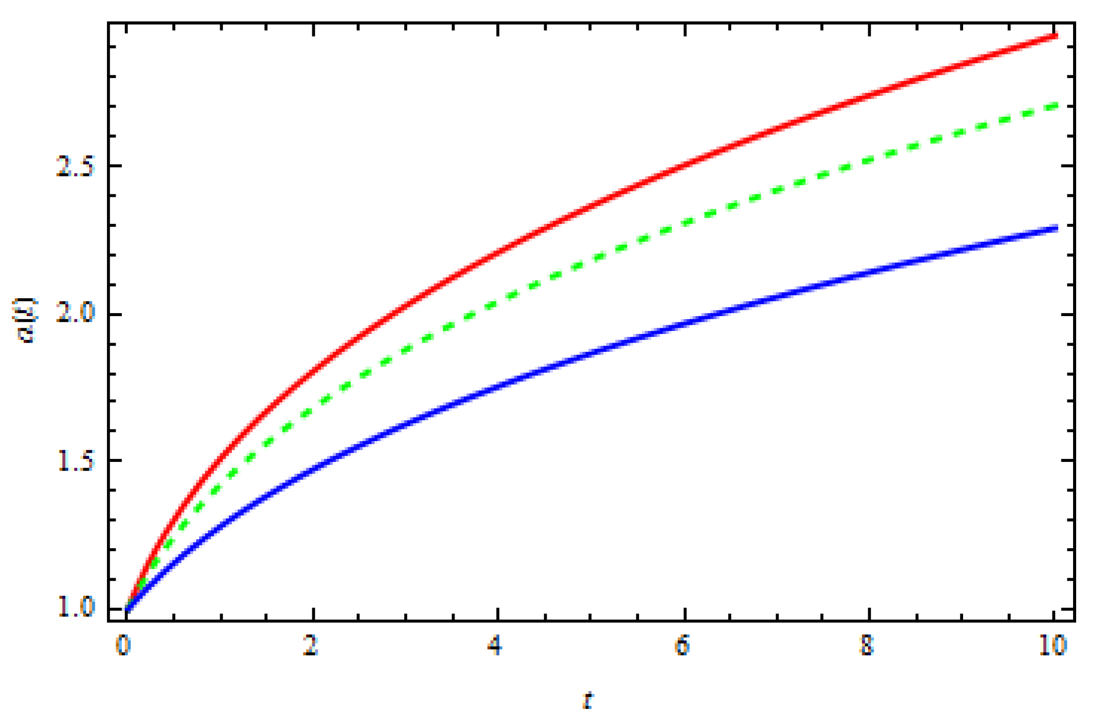
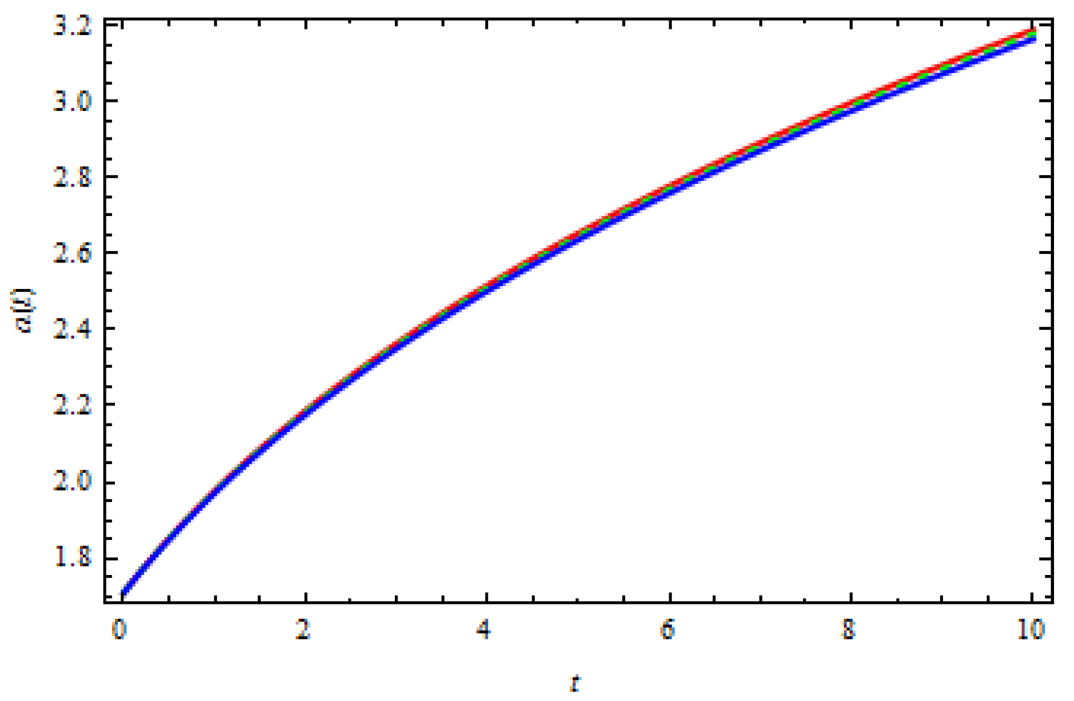
A graph of scale factor vs. temporal coordinate is plotted to investigate the behavior of the results obtained, with various values of $\alpha =0.7,\beta =0.5$ and $\omega =-1,-\frac{1}{3},0$ corresponding to red, green, and blue curves, respectively.

The Figure 1 is obviously shown that the increasing trends indicate that the universe is in an accelerating phase of expansion in the framework of CSMG theory.

Let us consider a case in which all the contributions from dark energy, pressure and mass density obey the law of conservation such that

$$\begin{array}{c}\hfill \dot{\rho }=-3\frac{\dot{a}}{a}(\rho +p).\end{array}$$

(33)

$p=\omega \rho$, thus Equation (33) becomes

$$\frac{\dot{\rho }}{\rho }=-3\frac{\dot{a}}{a}(1+\omega ).$$

(34)

The integral value of $\rho \left(t\right)$ is evaluated as

$$\rho \left(t\right)={ϵ}_2{\left[3\left(\sqrt{\frac{2(1+3\omega )ϵ}{3\left[6\right(-1-\omega \left)\right(\beta -\alpha )-(1-\omega \left)\right]}}\right)t+{ϵ}_1\right]}^{-(1+\omega )}.$$

(35)

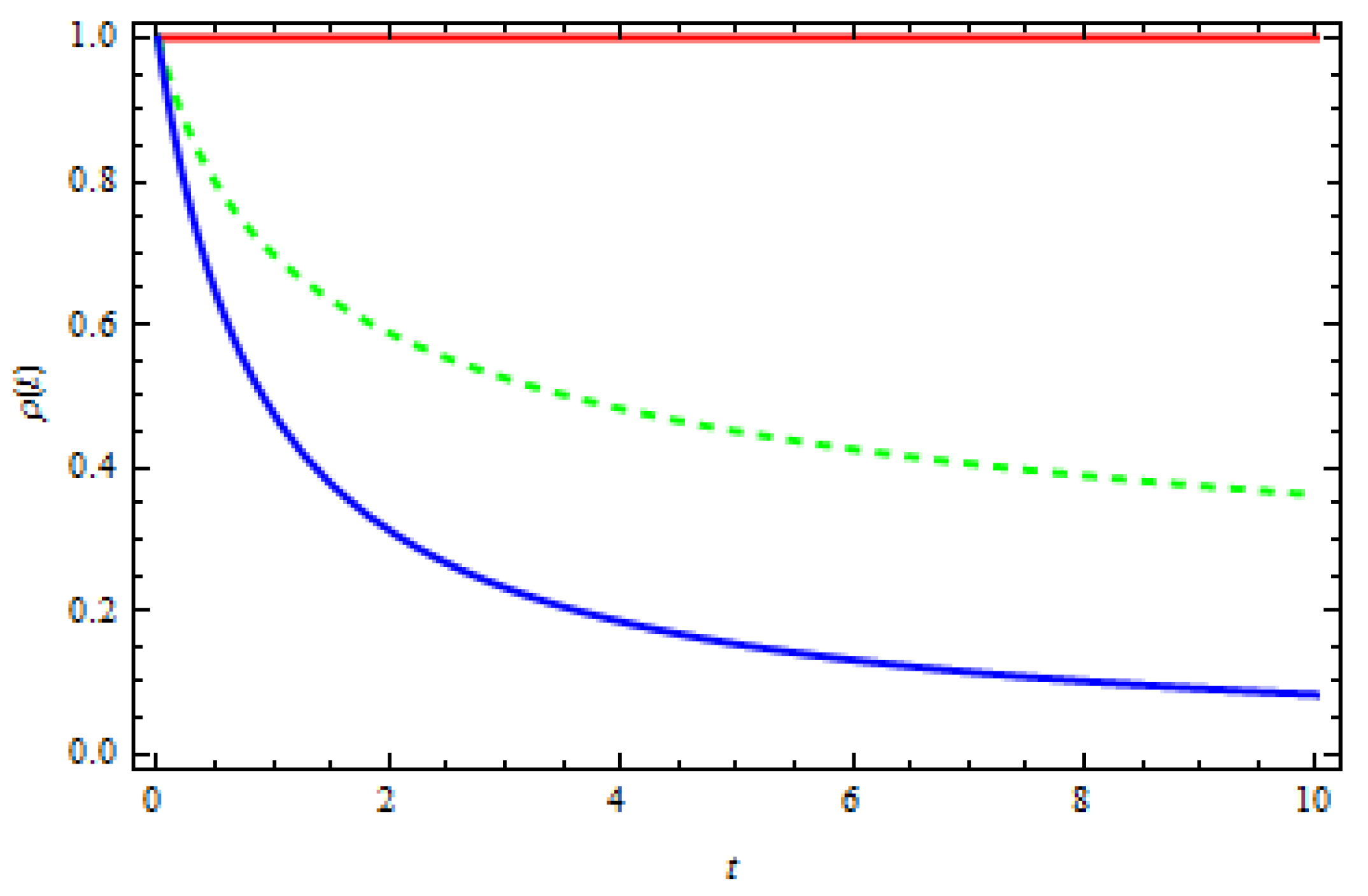
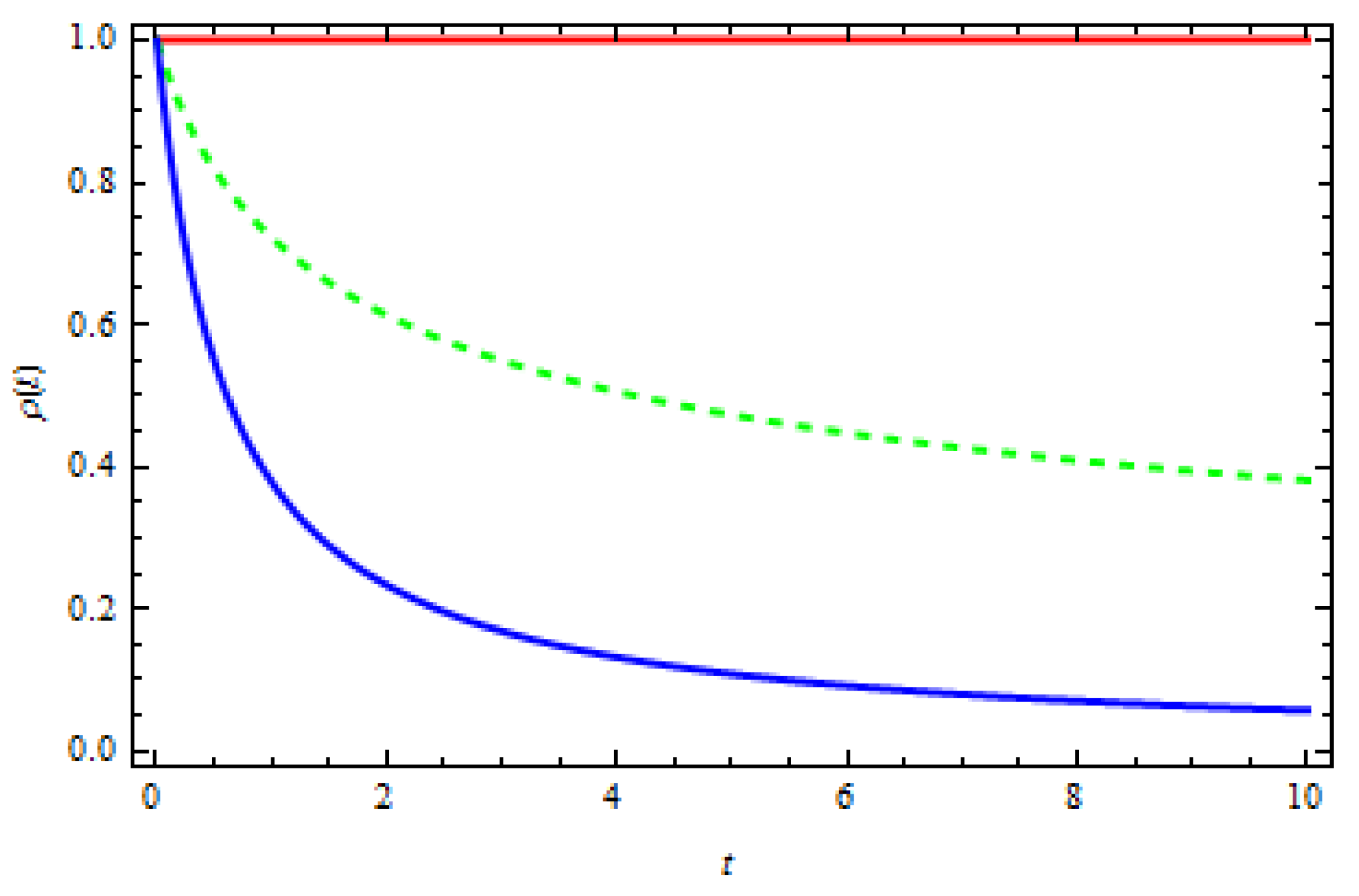
Let us plot a graph of Equation (35). The graphical representation of energy density vs. temporal coordinate makes a conjecture that decreases equally to the prediction of GR on considering a set of parametric values of $\alpha =0.7,\beta =0.5$ and $\omega =-1,-\frac{1}{3},0$ corresponding to red, green and blue curves respectively, in the context of CSMG theory in Figure 2.

Furthermore, to evaluate cosmological parameter $\Lambda \left(t\right)$ considered as the DE model, we use the values of energy density and scale factor, arriving at

$$\Lambda \left(t\right)=\frac{9{ϵ}^2+18(\alpha -2)(1+3\omega )}{81c^2(\alpha -\beta )[6(1+\omega )(\alpha -\beta )+(\omega -1)]}t+{ϵ}_1.$$

(36)

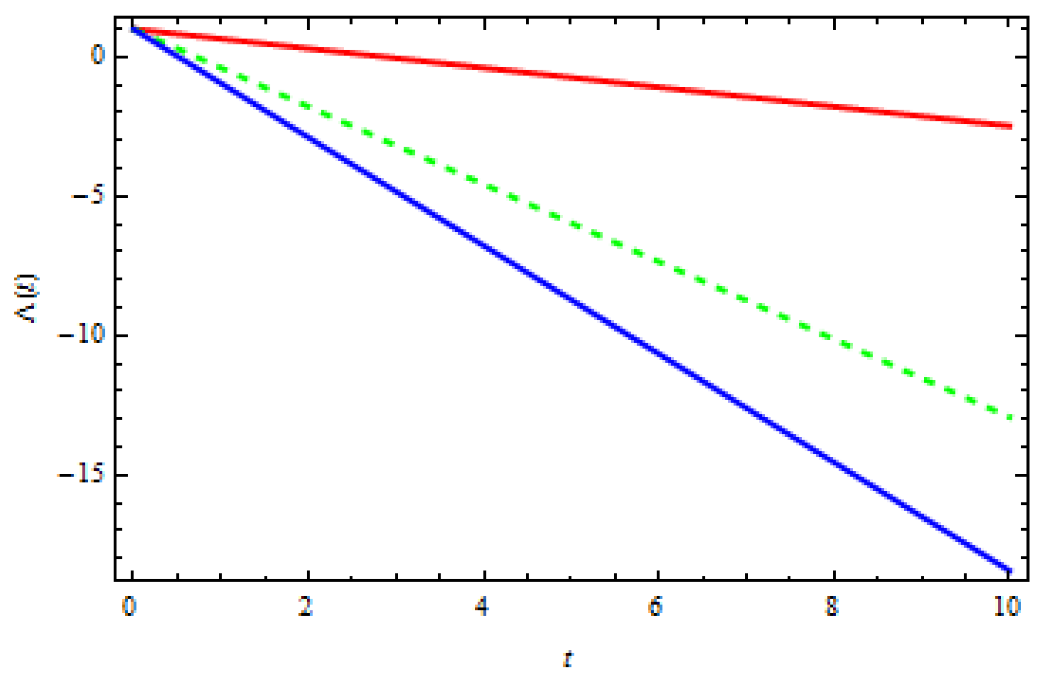
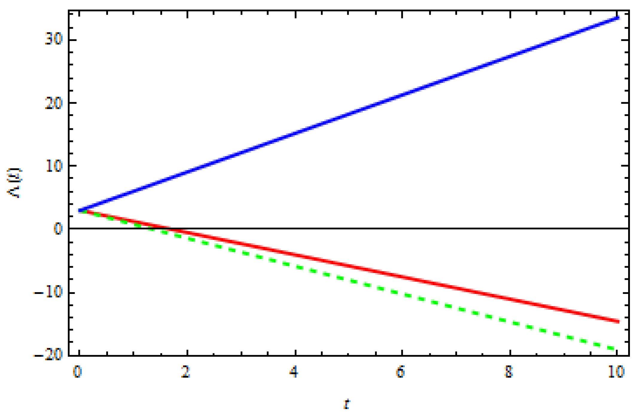
Now, to examine the cosmological constant $\Lambda \left(t\right)$ in the context of CSMG theory, a graph given in Figure 3 is plotted with previously assumed values.

It is well mentioned here that the graph of cosmological constant parameter $\Lambda \left(t\right)$ initiated from zero decreases as the cosmic time increases in the framework of CSMG theory. It is worth mentioning here that the graphical trends of $\Lambda \left(t\right)$ are decreasing described a decelerated expansion of the universe.

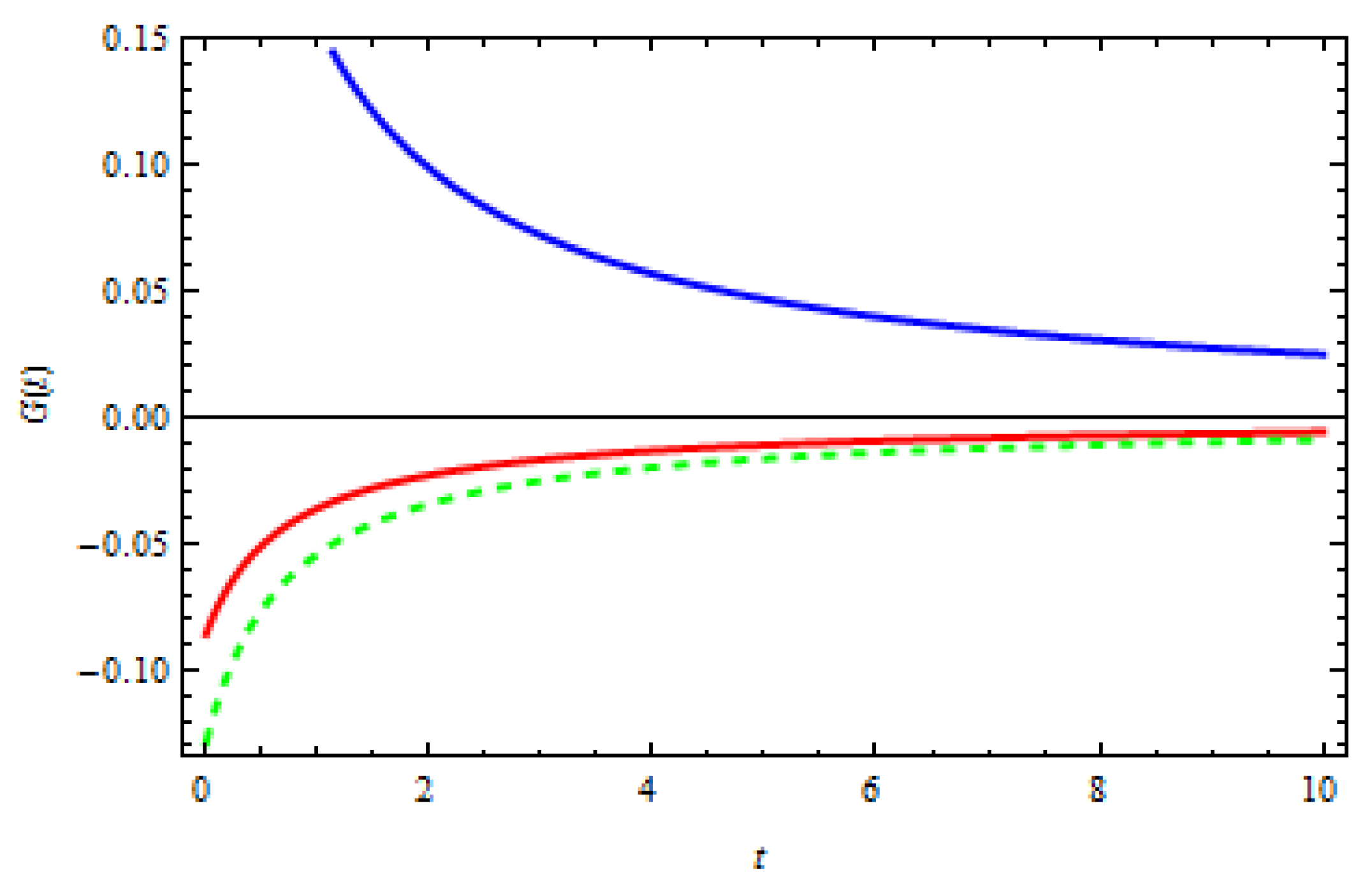
Using values of $\Lambda \left(t\right)$ and $\rho \left(t\right)$ from Equations (35) and (36), we obtain the mathematical relation for gravitational constant $G\left(t\right)$ such that

$$\begin{array}{ccc}\hfill G\left(t\right)& =& \frac{3(2-\beta )\frac{(1+3\omega )(\alpha -\beta )ϵ}{2(1+\omega )+\beta (1-3\omega )-4\alpha }-ϵ}{8\pi {ϵ}_1}\hfill \\ & \times & {\left[3\sqrt{\frac{(\alpha -\beta )(1+3\omega )}{2(1+\omega )+\beta (1-3\omega )-4\alpha }t}+{ϵ}_1\right]}^{-1}.\hfill \end{array}$$

(37)

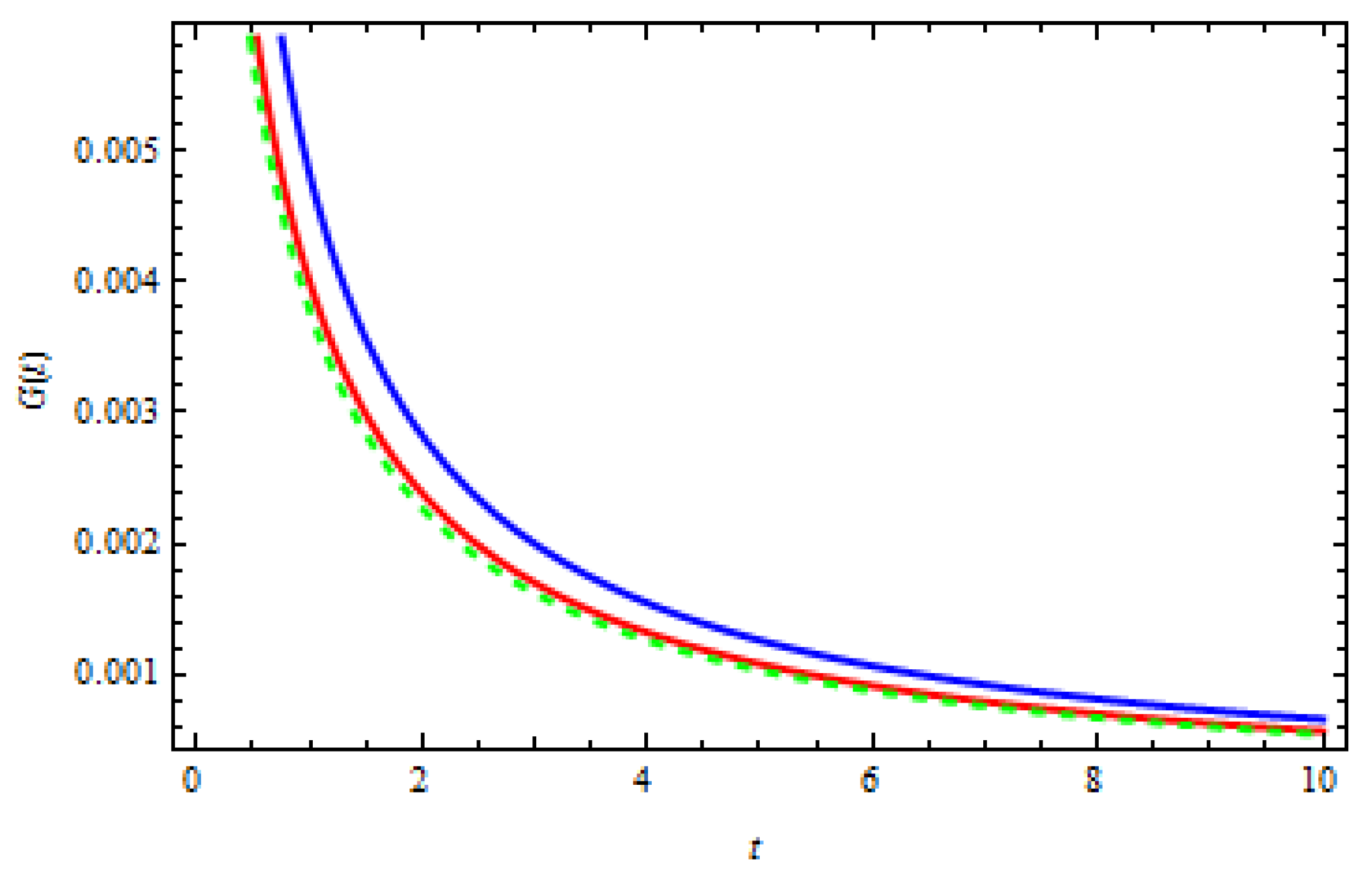
The graph of gravitational constant showed decreasing behavior, representing a contracting universe, as both $\Lambda \left(t\right)$ and $G\left(t\right)$ simultaneously decreased shown in Figure 4.

4. MHRDE Model

Gao et al. [12] proposed an interesting Ricci holographic dark energy (RHDE) model using the formula $L=\mid R{\mid }^{-\frac{1}{2}}$, where R is the Ricci scalar. The holographic principle in a cosmic scenario, by correlating the infrared cutoff L with the dark energy density and $L^{-2}$ as a linear combination of $\dot{H}$ and $H^2$, is given by $\Lambda =\frac{2}{\alpha -\beta }(\dot{H}+\frac{3}{2}\alpha H^2)$, where $\alpha$ and $\beta$ are free parameters. Substituting this model in Equations (22) and (23), new expressions are formulated as

$$4\pi G\rho =\frac{3}{2}(1-\frac{\alpha }{\alpha -\beta })H^2-\frac{1}{\alpha -\beta }\dot{H}-\frac{ϵa^{-6}}{2}.$$

(38)

$$3[\dot{H}+H^2]+4\pi \rho G(1+3\omega )=\frac{1}{\alpha -\beta }[2\dot{H}+3\alpha H^2].$$

(39)

Equations (38) and (39) simultaneously, these transformed into

$$\dot{H}=\frac{1}{2(\alpha -\beta )-(1+\omega )}[3(1+\omega )\beta H^2+(3+\omega )(\alpha -\beta )ϵa^{-6}].$$

(40)

Scale factor $a\left(t\right)$, Equation (40) takes the form

$$(\frac{\ddot{a}}{a})=\frac{3(1+\omega )\beta }{2(\alpha -\beta )-(1+\omega )}(\frac{\dot{a^2}}{a})+\frac{(\alpha -\beta )(3+\omega )}{2(\alpha -\beta )-(1+\omega )}ϵa^{-6}.$$

(41)

Substitutions $y\left(a\right)=\frac{da}{dt}\Rightarrow Y\frac{dY}{da}=\frac{d^{2}a}{d{t}^2}$ to calculate the scale factor, one arrives at

$$Y\frac{dY}{da}=\frac{3\beta (1+\omega )}{2(\alpha -\beta )-(1+\omega )}{y}^2+\frac{(3+\omega )(\alpha -\beta )}{2(\alpha -\beta )-(1+\omega )}ϵa^{-5}.$$

(42)

Use of substitution $U\left(a\right)=Y^2\left(a\right)\Rightarrow Y\left(a\right)\frac{dY}{da}=\frac{1}{2}\frac{dU}{da}$

$$\frac{dU}{da}-\frac{6(1+\omega )\beta }{2(\alpha -\beta )-(1+\omega )}U=\frac{2(3+\omega )(\alpha -\beta )}{2(\alpha -\beta )-(1+\omega )}ϵa^{-5}.$$

(43)

Equation can be evaluated as

$$U\left(a\right)=\frac{(\alpha -\beta )(3+\omega )ϵ}{-4\alpha +2(1+\omega )+(1-3\omega )\beta }\frac{1}{a^4}.$$

(44)

The technique of separating variables and using backward substitutions, the expression of scale factor $a\left(t\right)$ looks as follows:

$$a\left(t\right)={\left[3\left(\sqrt{\frac{(\alpha -\beta )(3+\omega )ϵ}{(-4\alpha +2(1+\omega )+\beta (1-3\omega \left)\right)}}\right)t+{ϵ}_1\right]}^{\frac{1}{3}}.$$

(45)

The scale factor and time graph is plotted in Figure 5 are plotted to investigate the obtained results, which obviously show the increasing behavior with time, predicting the accelerated phase of expansion of the universe.

Working on the same lines, we obtain

$$\rho \left(t\right)={\left[3\left(\sqrt{\frac{(\alpha -\beta )(3+\omega )ϵ}{(-4\alpha +\beta (1-3\omega )+2(1+\omega \left)\right)}}\right)t+{ϵ}_1\right]}^{-(1+\omega )}.$$

(46)

where ${ϵ}_1$ is the constant of integration. Now, we draw the energy density vs. time graph (Figure 6). The visual representation reveals that the density is decreasing with the passage of time, which is consistent with GR’s predictions.

The relation for cosomological constant $\Lambda \left(t\right)$ is given by

$$\Lambda \left(t\right)=\frac{9(\alpha -2)(\alpha -\beta )(1+3\omega )+{ϵ}^2}{3{ϵ}^2(\alpha -\beta )[-4\alpha +2(1+\omega )+\beta (1-3\omega )]}t+{ϵ}_1.$$

(47)

In Figure 7, the behavior of cosmological constant $\Lambda \left(t\right)$ in the CSMG theory shows a decreasing trend for $\omega =-1$ and $-\frac{1}{3},$ but increasing on $\omega =0$ as the cosmic time increases. The cosmological constant $\Lambda \left(t\right)$ is revealed to be a decreasing function, which is endorsed by observational data of recent type Ia supernovae. Addazi [43] argued that the holographic naturalness model prefers models over dynamical variation of $\Lambda$ toward a cosmological attractor $\Lambda ⟶0$ over models with a static cosmological constant. While a Big Rip is expected from the scenarios with $\Lambda$ increasing with time, it is entropically confiscated as a quantum unstable state.

The expression for gravitational constant $G\left(t\right)$ is evaluated as

$$\begin{array}{ccc}\hfill G\left(t\right)& =& \frac{\frac{(1+3\alpha -\beta )(3+\omega )(\alpha -\beta )ϵ}{2(1+\omega )+\beta (1-3\omega )-4\alpha }-c}{8\pi {ϵ}_1}\hfill \\ & \times & {\left[3\sqrt{\frac{(\alpha -\beta )(3+\omega )ϵ}{-4\alpha +2(1+\omega )+(1-3\omega )\beta }t}+{ϵ}_1\right]}^{-1},\hfill \end{array}$$

(48)

We plotted a graph between gravitational constant $G\left(t\right)$ and cosmic time t, in Figure 8 where increasing tendencies were seen in the visual representation of gravitational constant for varying parameters for $\omega =-1,-\frac{1}{3}$ but decreasing on $\omega =0$. The critical density assumption and the conservation of energy–momentum tensor demand that G increases proportionally for the expanding universe as found in [44].

5. Numerical Results and Comparison with Other Models

Štefančić [45] investigated the time-dependent $G\left(t\right)$ and discovered that it is more susceptible to the phantom energy component $\eta$. $G\left(t\right)$ varied slowly in the early cosmos, but the variability of $G\left(t\right)$ is astonishing in the current era, while $G\left(t\right)$ tends to zero over extended periods of time. For larger negative values of variable $\eta$, it changes very quickly. The escalating negative values of $\eta$ demonstrated to be an effective testing ground for several models. It would start imposing the stringent restrictions on the emergence of the cosmological constant, energy density, and scale factor, which are all depicted by the parameter $\eta$. Štefančić [45] founded the results for $\frac{\dot{G}}{G}$, given by

$$\frac{\dot{G}}{G}=3(1+\eta ){\Omega }_{\Lambda }^0{H}_0.$$

(49)

Equation (37) is related to the phantom energy model parameter $\eta$. We calculated, by following Equation (37),

$$\frac{\dot{G}}{G}=-3H.$$

(50)

Compare Equation (49) and Equation (50) along with ${\Omega }_{\Lambda }^0=\frac{2}{3}$ from recent observational data.

$$\eta =\frac{-5}{2}$$

(51)

The values of $\eta$ and ${\Omega }_{\Lambda }^0$ in (49), we explored the same result as found in Equation (50).

$$\frac{\dot{G}}{G}=-3H_0.$$

(52)

The gravitational constant $G\left(t\right)$ changes rapidly with negative values of $\eta$, according to Stefancic [45], and the same is apparently true in this study. Many astronomical observations have validated the fluctuation in the value of the gravitational constant as time progresses. Many of them have produced similar results, confirming Dyson’s claim that the variance of the values of the gravitational constant $G\left(t\right)$ is the Hubble parameter’s order. Because the Hubble parameter H is inversely proportional to the time coordinate t, $G\left(t\right)$ declines as t rises. Guenther et al. [46] used helioseismology data to determine the range of $\frac{\dot{G}}{G}$ and accumulated the comprehensive range of $G\left(t\right)$ variability, which is 1.60 $\times {10}^{-12}{\mathrm{yr}}^{-1}<\frac{\dot{G}}{G}<0$. Benvento [47] computed the range $-2.5\times {10}^{-10}{\mathrm{yr}}^{-1}<\frac{\dot{G}}{G}<4.5\times {10}^{-10}{\mathrm{yr}}^{-1}$. Damour et al. [48] employed binary pulsar data to compute the variation ranges for $\frac{\dot{G}}{G}$, and found $-\left(1.10\frac{+}{}1.07\right)\times {\mathrm{yr}}^{-1}<\frac{\dot{G}}{G}<0$. Biesiada and Malces [49] found the optimal variation range $\frac{\dot{G}}{G}<4.1\times {10}^{-11}{\mathrm{yr}}^{-1}$ via using observational data from dwarf stars. Copi et al. [50] computed $-4.1\times {10}^{-13}{\mathrm{yr}}^{-1}<\frac{\dot{G}}{G}<3.5\times {10}^{-13}{\mathrm{yr}}^{-1}$ through using Big Bang nuclei synthesis. Additionally, on the basis of experimental data from WMAP, Zhang and Wu [51] revised the current value of $H_0=6.64\times {10}^{-11}{\mathrm{yr}}^{-1}$. In this paper, using this numerical value, we calculated the range $-1.99\times {10}^{-10}{\mathrm{yr}}^{-1}\le \frac{\dot{G}}{G}\le 0$ equivalent to [52].

6. Summary and Discussion

In this study, we analyzed the time-dependent gravitational constant $G\left(t\right)$ and cosmological constant $\Lambda \left(t\right)$ in the context of Chern–Simons modified gravity theory using HDE and MHRDE models. The FRW metric was examined by calculating the scale factor, energy density, cosmological constant and gravitational constant. Addazi [43] argued that the holographic naturalness model prefers models over dynamical variation of $\Lambda$ toward a cosmological attractor $\Lambda ⟶0$ over models with a static cosmological constant. While a Big Rip is expected from the scenarios with $\Lambda$ increasing with time, it is entropically confiscated as a quantum unstable state. It is shown that the $\Lambda =H^3$ model predicts the accelerated expansion of the universe at a negative energy density, but with a positive pressure [53]. Further, we studied the $\frac{\dot{G}}{G}$ for both models with different limitations on variational values of $G\left(t\right)$ obtained from theoretical as well as observational data. It is found that $G\left(t\right)$ is inversely proportional to time such that $G\propto t^{-1}$ for all possibilities of $\frac{\dot{G}}{G}$ mentioned. Belinchon [54] obtained similar accuracy during the dimensional investigation employing on Dirac’s large number of the hypothesis (LNH) in the context of GR, i.e., $G\propto t$, which is obviously contrary to Dirac’s conclusion. However, $G\left(t\right)$ fluctuates inversely with t in the current investigations. Finally, it is observed that, regardless of the variability of the gravitational constant $G\left(t\right)$, the scale factor and cosmological constant preserved the same status for both the models considered in this paper. With the appropriate scaling of $\alpha$ and $\beta$, we estimated the range for variation of $G\left(t\right)$ given as $-1.99\times {10}^{-10}{\mathrm{yr}}^{-1}\le \frac{\dot{G}}{G}\le 0$, which matches [52].

References

- Riess, A.G.; Filippenko, A.V.; Challis, P.; Clocchiatti, A.; Diercks, A.; Garnavich, P.M.; Gilliland, R.L.; Hogan, C.J.; Jha, S.; Kirshner, R.P.; et al. Observational evidence from supernovae for an accelerating universe and a cosmological constant. Astron. J. 1998, 116, 1009. [Google Scholar] [CrossRef] [Green Version]
- Perlmutter, S.; Aldering, G.; Goldhaber, G.; Knop, R.A.; Nugent, P.; Castro, P.G.; Deustua, S.; Fabbro, S.; Goobar, A.; Groom, D.E.; et al. Measurements of Ω and Λ from 42 high-redshift supernovae. Astrophys. J. 1999, 517, 565–586. [Google Scholar] [CrossRef]
- Jackiw, R.; Pi, S.Y. Chern-Simons modification of general relativity. Phys. Rev. D 2003, 68, 104012. [Google Scholar] [CrossRef] [Green Version]
- Alexander, S.; Yunes, N. Chern-Simons modified general relativity. Phys. Rep. 2009, 480, 1–55. [Google Scholar] [CrossRef] [Green Version]
- Smith, T.L.; Erickcek, A.L.; Caldwell, R.R.; Kamionkowski, M. Effects of Chern-Simons gravity on bodies orbiting the Earth. Phys. Rev. D 2008, 77, 024015. [Google Scholar] [CrossRef] [Green Version]
- Li, M. A model of holographic dark energy. Phys. Lett. B 2004, 603, 1–5. [Google Scholar] [CrossRef]
- Sheykhi, A. Holographic Scalar Fields Models of Dark Energy. Phys. Rev. D 2011, 84, 107302. [Google Scholar] [CrossRef] [Green Version]
- Hu, B.; Ling, Y. Interacting dark energy, holographic principle and coincidence problem. Phys. Rev. D 2006, 73, 123510. [Google Scholar] [CrossRef] [Green Version]
- Ma, Y.Z.; Gong, Y.; Chen, X. Features of holographic dark energy under the combined cosmological constraints. Eur. Phys. J. C 2009, 60, 303. [Google Scholar] [CrossRef] [Green Version]
- Hsu, S.D.H. Entropy bounds and dark energy. Phys. Lett. B 2004, 594, 13–16. [Google Scholar] [CrossRef] [Green Version]
- Wei, H.; Zhang, S.N. Age Problem in the Holographic Dark Energy Model. Phys. Rev. D 2007, 76, 063003. [Google Scholar] [CrossRef] [Green Version]
- Gao, C.; Wu, F.; Chen, X.; Shen, Y.-G. Holographic dark energy model from Ricci scalar curvature. Phys. Rev. D 2009, 79, 043511. [Google Scholar] [CrossRef] [Green Version]
- Granda, L.N.; Oliveros, A. Infrared cut-off proposal for the holographic density. Phys. Lett. B 2008, 669, 275–277. [Google Scholar] [CrossRef] [Green Version]
- Granda, L.N.; Oliveros, A. New infrared cut-off for the holographic scalar fields models of dark energy. Phys. Lett. B 2009, 671, 199–202. [Google Scholar] [CrossRef] [Green Version]
- Karami, K.; Fehri, J. New holographic scalar field models of dark energy in non-flat universe. Phys. Lett. B 2010, 684, 61–68. [Google Scholar] [CrossRef] [Green Version]
- Wang, S.; Wang, Y.; Li, M. Holographic Dark Energy. Phys. Rep. 2017, 696, 1–57. [Google Scholar] [CrossRef] [Green Version]
- ťHooft, G. Dimensional reduction in quantum gravity. arXiv 1993, arXiv:gr-qc/9310026. [Google Scholar]
- Nojiri, S.; Odintsov, S.D. Covariant generalized holographic dark energy and accelerating universe. Eur. Phys. J. C 2017, 77, 528. [Google Scholar] [CrossRef]
- Nojiri, S.; Odintsov, S.D.; Saridakis, E.N. Modified cosmology from extended entropy with varying exponent. Eur. Phys. J. C 2019, 79, 242. [Google Scholar] [CrossRef]
- Nojiri, S.; Odintsov, S.D.; Saridakis, E.N. Holographic inflation. Phys. Lett. B 2019, 797, 134829. [Google Scholar] [CrossRef]
- Nojiri, S.; Odintsov, S.D.; Oikonomou, V.K.; Paul, T. Unifying holographic inflation with holographic dark energy. Phys. Rev. D 2020, 102, 023450. [Google Scholar] [CrossRef]
- Nojiri, S.; Odintsov, S.D.; Paul, T. Different faces of generalized holographic dark energy. Symmetry 2021, 13, 928. [Google Scholar] [CrossRef]
- Cai, R.G.; Hu, B.; Zhan, Y. Holography, UV/IR relation, causal entropy bound, and dark energy. Commun. Theor. Phys. 2009, 51, 954. [Google Scholar]
- Silva, J.G.; Santos, A.F. Ricci dark energy in Chern–Simons modified gravity. Eur. Phys. J. C 2013, 73, 2500. [Google Scholar] [CrossRef]
- Amir, M.J.; Ali, S. Ricci dark dnergy of Amended FRW universe in Chern-Simon modified gravity. Int. J. Theor. Phys. 2015, 54, 1362. [Google Scholar] [CrossRef] [Green Version]
- Ali, S.; Amir, M.J. Cosmological analysis of modified holographic Ricci dark energy in Chern-Simons modified gravity. Adv. High Energy Phys. 2019, 2019, 3709472. [Google Scholar] [CrossRef]
- Amir, M.J.; Ali, S. A study of holographic dark energy models in Chern-Simon modified gravity. Int. J. Theor. Phys. 2016, 55, 5095–5105. [Google Scholar]
- Pasqua, A.; da Rocha, R.; Chattopadhyay, S. Holographic dark energy models and higher order generalizations in dynamical Chern-Simons modified gravity. Eur. Phys. J. C 2015, 75, 44. [Google Scholar] [CrossRef] [Green Version]
- Moradpour, H.; Moosavi, S.A.; Lobo, I.P.; Graa, J.P.M.; Jawad, A.; Salako, I.G. Thermodynamic approach to holographic dark energy and the Rényi entropy. Eur. Phys. J. C 2018, 78, 829. [Google Scholar] [CrossRef]
- Porfirio, P.J.; Fonseca-Neto, J.B.; Nascimento, J.R.; Petrov, A.Y. On the causality aspects of the dynamical Chern-Simons modified gravity. Phys. Rev. D 2016, 94, 104057. [Google Scholar] [CrossRef] [Green Version]
- Konno, K.; Matsuyama, T.; Asano, Y.; Tanda, S. Flat rotation curves in Chern-Simons modified gravity. Phys. Rev. D 2008, 78, 024037. [Google Scholar] [CrossRef] [Green Version]
- Guarrera, D.; Hariton, A.J. Papapetrou energy-momentum tensor for Chern-Simons modified gravity. Phys. Rev. D 2007, 76, 044011. [Google Scholar] [CrossRef] [Green Version]
- Nandi, K.K.; Kizirgulov, I.R.; Mikolaychuk, O.V.; Mikolaychuk, N.P.; Potapov, A.A. Quantum phase shift in Chern-Simons modified gravity. Phys. Rev. D 2009, 79, 083006. [Google Scholar] [CrossRef] [Green Version]
- Ray, S.; Mukhopadhyay, U.; Choudhury, S.B.D. Dark energy models with a time-dependent gravitational constant. Int. J. Mod. Phys. D 2007, 16, 1791. [Google Scholar] [CrossRef] [Green Version]
- Sarfraz, A.; Saddique, M. Time Dependent Gravitational Constant in Chern Simons Modified Gravity. Iran. J. Phys. Res. 2021, 21, 3. [Google Scholar]
- Alfedeel, A.H.A.; Abebe, A.; Gubara, H.M. A generalized solution of Bianchi type-V models with time-dependent G and Λ. Universe 2018, 4, 83. [Google Scholar] [CrossRef] [Green Version]
- Alfedeel, A.H.A.; Abebe, A. Bianchi type-V solutions with varying and: The general case. Int. J. Geom. Methods Mod. Phys. 2020, 17, 2050076. [Google Scholar] [CrossRef]
- Cohen, A.G.; Kaplan, D.B.; Nelson, A.E. Effective field theory, black holes, and the cosmological constant. Phys. Rev. Lett. 1999, 82, 4971–4974. [Google Scholar] [CrossRef] [Green Version]
- Bartelmann, M. Gravitational lensing. Class. Quantum Grav. 2010, 27, 233001. [Google Scholar] [CrossRef] [Green Version]
- Kujat, J.; Angela, M.; Robert, L.; Scherrer, J.; Weinberg, H.D. Prospects for determining the equation of state of the dark energy: What can be learned from multiple observables? Astrophys. J. 2002, 572, 1. [Google Scholar] [CrossRef] [Green Version]
- Knop, R.A.; Aldering, G.; Amanullah, R.; Astier, P.; Blanc, G.; Burns, M.S.; Conley, A.; Deustua, S.E.; Doi, M.; Ellis, R.; et al. New constraints on ΩM, ΩΛ, and ω from an independent set of 11 high-redshift supernovae observed with the Hubble Space Telescope. Astrophys. J. 2003, 598, 102. [Google Scholar] [CrossRef] [Green Version]
- Tegmark, M.; Blanton, M.; Strauss, M.; Hoyle, F.; Schlegel, D.; Scoccimarro, R.; Vogeley, M.; Weinberg, D.; Zehavi, I.; Berlind, A.; et al. The 3D power spectrum of galaxies from the SDSS. Astrophys. J. 2004, 606, 70. [Google Scholar]
- Addazi, A. Holographic naturalness and cosmological relaxation. arXiv 2020, arXiv:2004.07988. [Google Scholar]
- Rahaman, A. A critical density cosmological model with varying gravitational and cosmological “Constants”. Gen. Relativ. Gravit. 1990, 22, 655–663. [Google Scholar] [CrossRef]
- Štefančić, H. Nonlinear density response and higher order correlation. Phys. Lett. B 2004, 595, 9. [Google Scholar] [CrossRef]
- Guenther, D.B.; Krauss, L.M.; Demarque, P. The age of globular clusters in light of hipparcos: Resolving the age problem? Astrophys. J. 1998, 2, 871. [Google Scholar] [CrossRef] [Green Version]
- Garcaa-Berro, E.; Isern, J. Astronomical measurements and constraints on the variability of fundamental constants. Astron. Astrophys. Rev. 2007, 14, 113–170. [Google Scholar] [CrossRef]
- Damour, T.; Gibbons, G.W.; Taylor, J.H. Equation of state and the maximum mass of neutron stars. Phys. Rev. Lett. 1988, 61, 1151. [Google Scholar] [CrossRef]
- Biesiada, M.; Malec, B. A new white dwarf constraints on the rate of chage of gravitational constant. Mon. Not. R. Astron. Soc. 2004, 350, 644–648. [Google Scholar] [CrossRef] [Green Version]
- Štefančić, H. Phantom appearance of non-phantom matter. Eur. Phys. J. C 2004, 36, 523–527. [Google Scholar] [CrossRef]
- Zhang, X.; Wu, F.Q. Constraints on holographic dark energy from type Ia supernova observations. Phys. Rev. D 2005, 72, 043524. [Google Scholar] [CrossRef] [Green Version]
- Gaztanaga, E.; Berro, E.G.; Isern, J.; Bravo, E.; Dominguez, I. Bounds on the possible evolution of the gravitational constant from cosmological type-Ia supernovae. Phys. Rev. D 2001, 65, 023506. [Google Scholar] [CrossRef] [Green Version]
- Ray, S.; Khlopov, M.; Mukhopadhyay, U.; Pratim Ghosh, P. Phenomenology of Lambda-CDM model: A possibility of accelerating Universe with positive pressure. Int. J. Theor. Phys. 2011, 50, 939. [Google Scholar] [CrossRef] [Green Version]
- Belinchón, J.A. Cosmological models with ‘some’ variable constants. Astrophys. Space Sci. 2002, 281, 765–775. [Google Scholar] [CrossRef]
Figure 1.
vs. t.
Figure 2.
Figure 3.
Figure 4.
Figure 5.
Figure 6.
Figure 7.
Figure 8.
Publisher’s Note: MDPI stays neutral with regard to jurisdictional claims in published maps and institutional affiliations. |
© 2022 by the authors. Licensee MDPI, Basel, Switzerland. This article is an open access article distributed under the terms and conditions of the Creative Commons Attribution (CC BY) license (https://creativecommons.org/licenses/by/4.0/).
Share and Cite
MDPI and ACS Style
Ali, S.; Saif, M.; Khan, K.A.; Shah, N.A.; Weera, W. A Note on Varying G and Λ in Chern–Simons Modified Gravity. Symmetry 2022, 14, 1430. https://doi.org/10.3390/sym14071430
AMA Style
Ali S, Saif M, Khan KA, Shah NA, Weera W. A Note on Varying G and Λ in Chern–Simons Modified Gravity. Symmetry. 2022; 14(7):1430. https://doi.org/10.3390/sym14071430
Chicago/Turabian StyleAli, Sarfraz, Maryam Saif, Khuram Ali Khan, Nehad Ali Shah, and Wajaree Weera. 2022. "A Note on Varying G and Λ in Chern–Simons Modified Gravity" Symmetry 14, no. 7: 1430. https://doi.org/10.3390/sym14071430
Note that from the first issue of 2016, this journal uses article numbers instead of page numbers. See further details here.