Modeling and Evaluation of the Susceptibility to Landslide Events Using Machine Learning Algorithms in the Province of Chañaral, Atacama Region, Chile

Abstract

Landslides represent one of the main geological hazards, especially in Chile. The main purpose of this study is to evaluate the application of machine learning algorithms (SVM, RF, XGBoost and logistic regression) and compare the results for the modeling of landslide susceptibility in the province of Chañaral, III region, Chile. A total of 86 sites are identified using various sources, in addition to 86 non-landslide sites. This spatial data management and analysis are conducted using QGIS software. The sites are randomly divided, and then a cross-validation process is applied to calculate the accuracy of the models. After that, from 22 conditioning factors, 12 are chosen based on the information gain ratio (IGR). Subsequently, five factors are excluded by the correlation criterion. After this analysis, two indices not previously utilized in the literature, the NDGI (normalized difference glacier index) and EVI (enhanced vegetation index), are employed for the final model. The performance of the models is evaluated through the area under the ROC (receiver operating characteristic) curve (AUC). To study the statistical behavior of the model, the Friedman nonparametric test is performed to compare the performance with the other algorithms and the Nemenyi test for pairwise comparison. Of the algorithms used, RF (AUC = 0.957) and XGBoost (AUC = 0.955) have the highest accuracy values measured in AUC compared to the other models and can be used for the same purpose in other geographic areas with similar characteristics. The findings of this investigation have the potential to assist in land use planning, landslide risk reduction, and informed decision making in the surrounding zones.

1. Introduction

Geological hazards constitute one of the greatest impacts that global and local economies, as well as human settlements, may face [1,2]. In particular, landslides, which are defined as movements of soil, mud, debris, or rock, are the most common geological hazard in the world [3]. Landslides are a major hazard to human life and property since they occur all over the world and are characterized by a vast effect, sudden onset, and multiple instances [4]. They are commonly induced by natural events such as earthquakes or heavy rainfall, which occur in specific geological, geomorphological, and hydrological environments. In mountainous areas, landslides can have significant effects on topographic features, forests and soil, as well as on infrastructure such as roads and farming land.

The extent of these effects will depend on the magnitude of the landslides [5,6]. In the last two decades, efforts to assess landslides have focused on studying susceptible zones and understanding the mechanisms that govern landslides ([7,8]). This has made it possible to extract valuable knowledge from the analysis of geomorphological, tectonic, geological, climatic, and anthropomorphic characteristics ([9]).

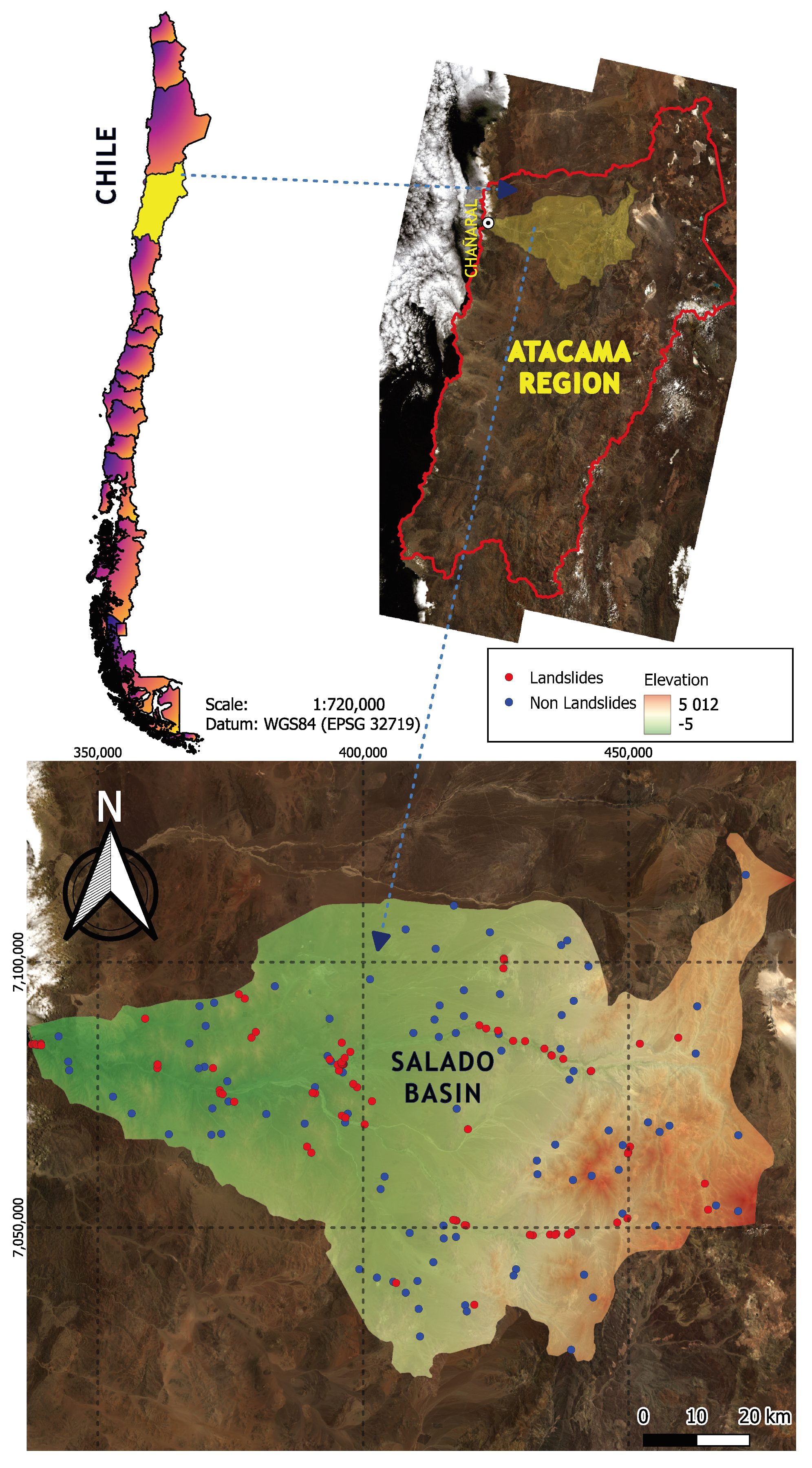
In Chile, landslides are one of the most common geological hazards, together with earthquakes, volcanic activity, and floods. The geological, geomorphological, tectonic, and climatic conditions of the country, characterized by the presence of the Andes Mountain Range on its eastern margin and the Coastal Mountain Range on its western margin, make it highly susceptible to the generation of mass movements such as landslides, rockfalls, flows, and falls [10]. Within 52 declared events in Chile, there have been a total of 1010 fatal victims caused by landslides, corresponding to 882 deaths and 128 people missing between 1928 and 2017 (90 years) [11]. The Atacama Region is characterized by a geomorphology that renders it susceptible to landslide events. According to documented records, this region has witnessed the highest number of fatalities resulting from flow-type events in the country, with a total of 132 people [11]. In the area of study, the Salado River basin, situated in the Chañaral Province of the region, a landslide event occurred in 1940 that resulted in the destruction of houses and the interruption of roads, causing substantial disruption to the city of Chañaral. In 1972, another landslide affected Chañaral and towns upstream, which were flooded, and 700 people were affected in Chañaral and 400 people in El Salado. Another flood in 1983 affected the city due to a rise in the river level caused by an increase in rainfall [12]. In Chañaral, there have been at least 15 major landslide events in the last 150 years [13]. With regard to the reports of deadly events and economic damage provoked by landslides, the identification of areas prone to these types of events and the determination of their risk level are the most critical actions in the assessment of the hazard [14].

In the last two decades, extensive research has been carried out on landslide methods using innovative technologies and tools to promote this field, such as in crisis management in mountain areas or near them [15]. Therefore, in order to obtain a reliable and accurate vulnerability map, it is necessary to test and evaluate several quantitative methods for more effective management of mountainous areas [16]. The use of Geographical Information Systems (GIS) in the elaboration of susceptibility maps constitutes an effective method to identify and delineate landslide-prone areas. This allows for the creation of a geospatial database of occurrences or an exhaustive inventory. By using GIS data repositories, the geospatial attributes of landslide-prone sites that can influence the potential stability of slopes, called landslide conditioning factors (LCFs), can be aggregated into a database.

Several methodologies and techniques have been developed for hazard susceptibility cartography around the world. The literature has classified them into ([14,17]):

• Models founded on physical conditions [18].
• Models founded on expert knowledge ([19,20]).
• Multivariate statistical methods. The examples are the statistical index (SI) [21], the frequency ratio (FR) ([22,23]), and logistic regression ([24,25]).
• Machine learning models, such as decision trees (DT) [26], random forests (RF) [27], support vector machines (SVM) [28], artificial neural networks (ANN) [22], and some hybrid methods, which include optimization algorithms ([7,16,24,29]).

Each of the methods described has its own unique strengths and limitations. Physical models, for example, require extensive field analysis and are currently considered unbeatable in terms of prediction accuracy, making them suitable for local-scale mapping. In order to work effectively, these models demand a complete knowledge of the landslide systems, obtained through meticulous observation and monitoring of the surface and the subsurface; this is essential in order to issue timely warnings of further slope collapse [30]. However, when applied on a larger scale, the need for a large amount of substantial data to obtain reliable results becomes inconvenient due to the considerable financial and computational resources required. Therefore, the use of this technique for the segmentation of larger regions is not feasible. This has led to the proliferation of statistical and knowledge-based models for more than four decades [31]. The knowledge-based models operate on the premise of building a framework with limited information, which is then parameterized by a system of weights assigned to factors according to expert judgment. Statistical models, on the other hand, have benefited from recent advances in GIS. This has paved the way for the successful application of a set of tools and quantitative methodologies for the modeling of landslides, improving in this way the understanding of the associated patterns and the causative agents [32]. At the moment, the thin line that separates statistical models from machine learning is a subject of controversy ([17,33]). The synergy and differences between statistical methods and machine learning are not clearly explained in academic works, mainly because the approach for geoscientists is primarily to generate and refine accurate results in landslide susceptibility mapping (LSM) rather than algorithmic categorization. In essence, machine learning is characterized by its ability to extract knowledge from data without relying on rule-based functions, whereas statistical modeling aims to establish relationships between data variables through algebraic expressions. Although the two fields were once considered mutually exclusive, they have recently converged [17]. A notable example is the adoption of the logistic regression (LR) algorithm, originally from statistics, to solve classification problems. Now, machine learning has adopted LR and has become one of the most widely used algorithms. However, machine learning is more concerned with optimization and efficiency, in contrast to the inferential approach of statistical models.

Machine learning methods have been used in engineering and science problems for more than two decades. This is the reason why the use of these techniques in the area of geosciences and remote sensing is quite new and limited. Machine learning focuses on the automatic extraction of information from data through computational and statistical methods. The areas of applicability are very diverse and involve different topics such as rock mass characterization, ocean products, vegetation indices, etc. At present, data analysis methods play a central role in geosciences and remote sensing. While collecting large volumes of data is essential in the field, the analysis of this information becomes a major challenge [34]. Various machine learning techniques, including random forests (RF), support vector machines (SVM), and artificial neural networks (ANN), have proven to be effective in dealing with nonlinear data across different scales in areas such as identification, prediction, mitigation, and modeling. Studies like [6,35,36] and others have demonstrated the success of these methods. Unlike traditional statistical models, which aim to infer relationships between variables, machine learning models autonomously identify logical criteria from input data to make highly accurate predictions [35]. The primary benefits of machine learning are its accuracy and ability to capture nonlinear correlations, as well as its ability to successfully overcome the impacts of various data distributions [37], flexibility (these models can be adapted to different types of data and problems), speed (they can process large amounts of data quickly and efficiently), and generalization (once the model is trained, it can be applied to new data to produce reliable predictions).

There are several research gaps in the modeling of landslide susceptibility using machine learning algorithms. Some of them are the following:

• Integration of multiple factors: Most studies have focused on assessing a limited and repetitive set of factors. The integration of new factors needs to be explored to improve model accuracy and ensure a more complete assessment of susceptibility.
• Development of interpretable models: Although machine learning models can achieve high accuracy in identifying landslide susceptibility, some of these models can be difficult to interpret and explain. There is a need to develop interpretable models that allow decision makers to understand how the data are being used and how susceptibility identification is being performed [38].
• The lack of simplification of the models in terms of the use of factors: Many models rely on multiple data sources, such as area-specific maps (geology, soils, roads, etc.), which hinder subsequent reproducibility and detract from some dynamic dimension of the model, which, if only satellite parameters and/or digital elevation were used, could be updated as these images become available.

In this work, we seek to fill one of the existing research gaps in the Central Andes, in the sense that there are few studies that characterize the susceptibility to landslides, which can help to understand the development of this phenomenon and thus apply the models generated in similar areas that have not yet been studied. For its part, the research question that this study seeks to address is how different machine learning techniques can be applied and compared to assess and predict susceptibility to landslides in a region of the Andes where no studies of this type have been carried out before.

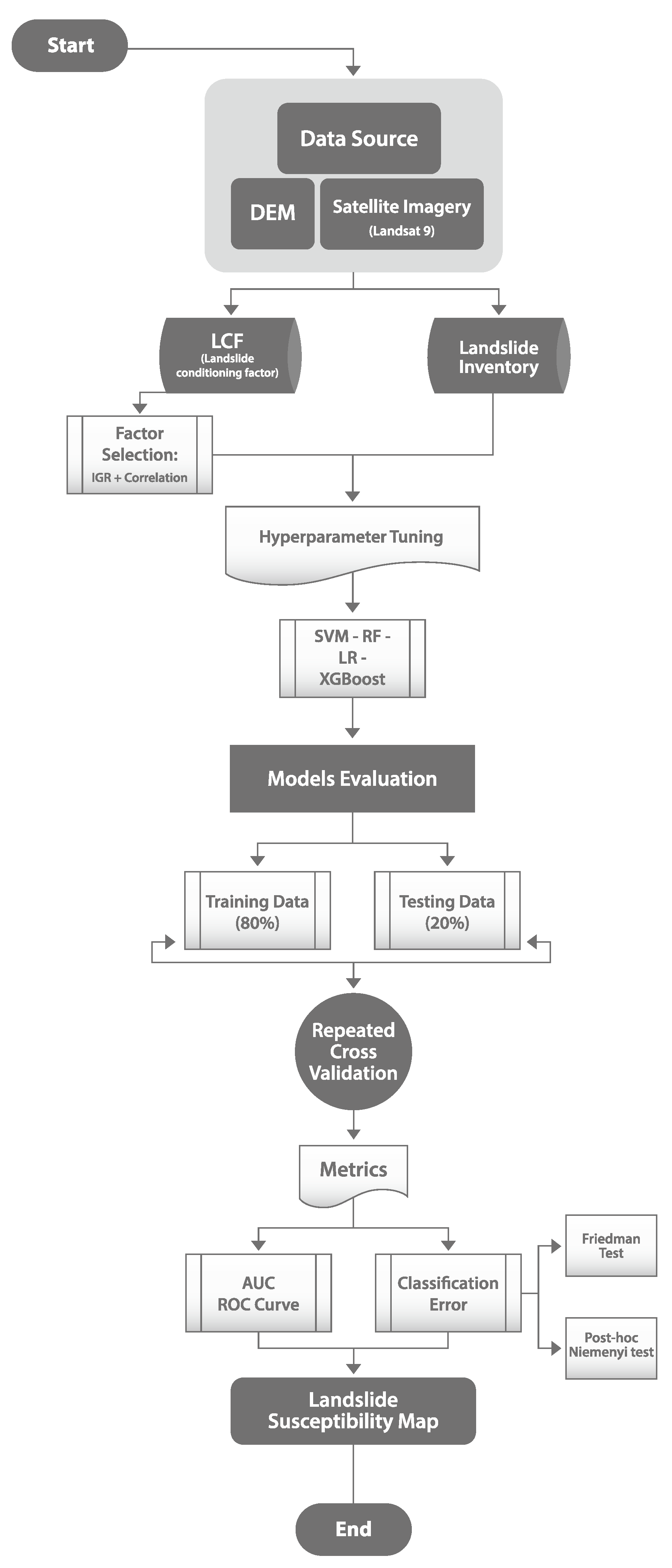
The objectives of the work are to build a susceptibility model of the Chañaral province to identify the areas most exposed to landslide risk by using machine learning algorithms (SVM, RF, XGBoost, and LR) and by comparing their performance; to build an inventory of landslides in the study area through historical records and the analysis of satellite images; and to determine the most relevant factors in susceptibility assessment by using indices based on information theory.

2. Materials and Methods

2.1. Study Area

The study area is the Salado river basin located in the Province of Chañaral (26.4° S), Atacama region, Chile, between longitudes 70.7° E and 69.5° E and latitudes 26.2° S and 27° S (Figure 1). In topographic and physical terms, the average altitudes range between 1000 and 1500 m above sea level. The geology of the Salado River basin is distinguished by an ancient basement composed of Paleozoic metamorphosed sedimentary rocks (Chañaral epimetamorphic complex). This complex is located near the coast and has been eroded over time by several minor streams, especially the Salado River. In addition, there are strips of Paleozoic intrusions, such as the batholiths of the Quebrada del Castillo. The presence of several intrusive bodies and two significant north–south regional fault systems (the Atacama Fault System to the west and the Domeyko Fault System to the east) indicate that the area has experienced intense volcanic and tectonic activity. In the study area, volcanosedimentary rocks of the La Negra Formation and the Punta del Cobre Group outcrop. These geological units are found in the center and south of the intermediate depression and to the west of the basin [39]. On the other hand, the Cenozoic era is characterized by sedimentary rocks that represent the ancient relief at the foot of the mountain range. These rocks denote greater compaction due to their age and are associated with the Miocene–Pliocene. The more recent natural and anthropogenic deposits, which show a lower degree of compaction, outcrop on the slopes and riverbeds that cross the basin. These deposits are variable in composition and are generally thin in narrower areas and thicker in more open areas. Landslides have mainly occurred on these geological formations [40].

The types of landslides found in this region correspond to alluviums and debris flows and are rainfall-induced landslides. According to the climatic classification, the area of study is in the transitional area between the hyperarid and semiarid zones [12]. Rainfall averages 1.7 mm per year in the lower zone of the basin and can reach up to 52 mm per year in the upper zone, where it accumulates between June and August, and the average temperature is between 10 and 20 °C for the coastal and medium-arid zones and −1.7 °C in the high-altitude zone [41].

2.2. Landslide Inventory Map

To examine the correlation between the spatial prediction of landslides and the relevant influencing factors, it is imperative to consider the most recent landslide records available. Consequently, to establish a comprehensive and reliable inventory for the study area, information from previous studies will be used and subsequently verified by laboratory analysis. The location of landslides was recorded through the analysis of the Sernageomin database, bibliographic search and interpretation of aerial photographs, and satellite images extracted from Sentinel Hub and the Copernicus repository, as well as the use of the Google Earth program. For the execution of the work, 86 locations of landslide events in the area of study were used, and another 86 locations were used as points where no landslides occurred. The information of this data set is included as supporting information with this manuscript. The validation corresponds to field visits by professionals from the agency and the respective visual inspection carried out by the researchers present in the study based on the analysis of aerial images obtained from Google Earth. The information is managed together through the free software QGIS version 3.22 and scripts created in R that contain the necessary instructions for the geospatial processing of the data and the extraction of characteristics. Also, in [32], it is suggested that by using samples from the landslide scarp polygon, it is possible to increase the accuracy of the model. In this work, the center of the landslide body was being used to characterize the phenomenon. Therefore, to increase the data set, it was decided to take ten samples (pixels) within the scarp polygon of each landslide, and in the case of the non-landslide points, a polygon surrounding the initial point was created, and from this, 10 samples were taken within this polygon, which allowed us to multiply by 10 the studied data set and thus provide the statistical robustness needed in this work. On the other hand, the points that were predicted correspond to ten million randomly chosen points within the study basin, which were rescaled to generate a raster that represents the susceptibility map.

2.3. Landslide Conditioning Factors

In this study, 22 factors related to the landslides were used, mainly obtained from the DEM of the AW3D30 project [42] and their respective analyses through R and multiple geoprocessing packages (geomorphological factors), in addition to optical satellite imagery received from the LANDSAT 9 campaign [43], which includes eleven spectral bands that can be combined to identify characteristics in the ground. The spectral bands are then manipulated to produce spectral index factors, which are multiple combinations of these bands. For the machine learning analysis and the respective algorithms, the data associated with each factor are included and then analyzed using R. Unlike other studies, this work focuses exclusively on two data sources, simplifying the methodology and opening the possibility for future applications in real-time monitoring.

Table 1. Factors derived from JAXA ALOS World 3D (30 m).

Factor	Definition	Reference
Elevation	Height over the sea level	[44]
Aspect	The direction to which a slope faces, typically expressed in degrees from north	[45]
Hillshade	A measure of the exposure of a surface to sunlight, based on the orientation and angle of the sun	[46]
Slope	Steepness of the land surface	[47]
Total curvature	A measure of the curvature of the ground surface that takes into account both the maximum and minimum curvature at each point	[48]
Plane curvature	Curvature of the ground surface in the direction of the horizontal plane	[48]
Topographic wetness index (TWI)	Indicator of the accumulation of moisture in the soil, calculated from the ratio of the cumulative flux to the slope of the land	[49]
Terrain ruggedness index (TRI)	A measure of the elevation variation in a region, indicating the roughness of the terrain	[50]
Topographic position index (TPI)	A value that compares the elevation of a point to the average elevation of a surrounding area	[51]
Slope length	Distance over which water flows before reaching a channel	[52]
Melton ruggedness number	A measure of terrain roughness that combines elevation height with watershed area	[53]
Convergence index	Index that evaluates the trend of convergence or divergence of water flow at the land surface	[51]
Valley depth	Vertical distance from the valley floor to the nearest peak	[54]
LS factor	Component of the revised universal soil loss equation (RUSLE) erosion prediction model representing slope length and slope gradient	[55]
Geomorphons	Terrain classification based on geomorphological patterns describing the shape of the terrain	[15]

and

Table 2. Factors derived from Landsat 9 L2 (10 m).

Factor	Definition	Reference
Normalized difference vegetation index (NDVI)	A spectral index that measures the density and health of vegetation based on the difference between the near-infrared and red bands	[56]
Green normalized difference vegetation index (GNDVI)	Variant of NDVI using the green band instead of the red band for greater sensitivity to differences in chlorophyll	[57]
Enhanced vegetation index (EVI)	Index similar to NDVI that corrects for some atmospheric and soil factors to improve vegetation monitoring	[58]
Normalized difference moisture index (NDMI)	Index designed to detect water stress in vegetation and drought conditions	[59]
BI (Bare soil index)	Index used to identify and quantify areas of bare soil	[60]
Normalized difference water index (NDWI)	An index that uses spectral information to identify and monitor moisture content in vegetation and water bodies	[61]
Normalized difference glacier index (NDGI)	Index used to detect and monitor glaciers and snow using spectral data	[62]

summarize the factors and the types of classes into which they can be classified, for reference. In addition, Figure 2, Figure 3 and Figure 4 show thematic maps of all the factors presented in this study together with the landslide inventory.

2.3.1. Geomorphological Factors

From the digital elevation model, it is possible to obtain a series of factors that correspond to functions derived from the topographic model, which have been used in the literature for the modeling of landslide susceptibility. Elevation influences the stability of slope materials by influencing local climate, geological conditions, and human accessibility to various places [44]. Because of factors like steep slopes, loose soil, and heavy rainfall, landslides are typically more common at higher elevations ([49,63]). Also, in landslide susceptibility mapping, slope is important because it affects water flow and material sliding [47]. At the same time, given its relationship to a number of other variables, such as rainfall and solar radiation, aspect is a topography element that is frequently used in landslide susceptibility mapping [45]. Another important component of landslide susceptibility mapping is hillshade, which indicates the relative location of the slope angle and clarifies a cell’s position with regard to its aspect and slope [46]. The curvature, both planar and total, is the rate at which the slope changes direction. There is a greater chance of unstable rock and soil conditions on high, curved slopes, which raises the susceptibility of landslides [48]. Another variable, the TRI (terrain ruggedness index), is introduced, and it measures the disparity in elevation values between a central cell and its eight surrounding cells [50]. The capacity of road flow to transport sediment is expressed in terms of slope length (SL) [52]. The convergence index is a useful tool for quantifying the divergence of the flow in the grid cells and is often used to analyze slope curvature [51]. TWI (topographic wetness index), another important influencing factor, was selected because of its association with the interaction of topography and moisture, which can impact the occurrence of landslides [49]. The terrain positioning index (TPI) is a measure that compares the elevation of each pixel with the average elevation of the neighboring pixels. [51]. The LS factor quantifies the impact of topography on the process of soil erosion [55]. The Melton coefficient is a metric that quantifies the roughness and average slope of a basin by considering flow accumulation. This statement indicates that it demonstrates the characteristics of the catchment area and its susceptibility to landslides [53]. Valley depth (VD) refers to the vertical distance between a specific point and the base level of the channel network. It plays a crucial role in slope stability and consequently influences the likelihood of landslides [54]. Finally, geomorphons are a landform classification that can be used to assist in landslide susceptibility prediction. Their application allows for a detailed classification of terrain features, such as ridges and valleys, thus facilitating a better understanding of geographical features that may influence landslide occurrence [15].

2.3.2. Spectral Factors

The spectral factors obtained from Landsat 9 satellite images represent normalized combinations of bands that enable the extraction of information regarding various characteristics of the study area. These factors can also be utilized in the assessment of susceptibility to landslides. The images were acquired in February 2022, and the ones utilized in this study are as follows:

• NDVI (normalized difference vegetation index): The NDVI is a factor that uses the red and the near-infrared band (NIR), and describes plant growth and coverage. The higher the vegetation coverage, the higher the NDVI value, and the lower the possibility of landslide [56].

  $$NDVI=\frac{NIR-Red}{NIR+Red}$$

  (1)
• GNDVI (green normalized difference vegetation index): This is a widely employed vegetation index that serves to assess photosynthetic activity and is commonly utilized for determining the water and nitrogen consumption of vegetation cover. The relationship with landslides is very similar in comparison with the NDVI index [57].

  $$GNDVI=\frac{NIR-Green}{NIR+Green}$$

  (2)
• EVI (enhanced vegetation index): The EVI exhibits greater sensitivity to changes in canopy structure, canopy composition, and plant morphology compared to the NDVI. The EVI is also correlated with stress and alterations associated with drought. Low EVI values can suggest regions with scarce or deteriorated vegetation, which could be a sign of heightened susceptibility to landslides [58].

  $$EVI=2.5\ast \frac{NIR-Red}{NIR+6\ast Red-7.5\ast Blue+1}$$

  (3)
• NDMI (normalized difference moisture index): This index is utilized for the assessment of vegetation water content [59].

  $$NDMI=\frac{NIR-SWIR}{NIR+SWIR}$$

  (4)
• BI (bare soil index): The reliability of the NDVI index diminishes in situations where the vegetation covers less than 50% of the area. To enhance the accuracy of vegetation status estimation, novel techniques incorporate a bare soil index (BI) that utilizes medium-infrared data. The fundamental rationale of this approach relies on the strong interdependence between the condition of exposed soil and the condition of vegetation. By integrating both vegetation and bare soil indices in the analysis, one can evaluate the state of forestlands along a spectrum that spans from abundant vegetation to uncovered soil conditions [60].

  $$BI=\frac{(SWIR1+Green)-(NIR+Blue)}{(SWIR1+Green)+(NIR+Blue)}$$

  (5)
• NDWI (normalized difference water index): The normalized difference Water Index (NDWI) is employed for the purpose of monitoring alterations associated with the water content in aquatic environments. The NDWI utilizes the green and near-infrared bands to emphasize water bodies, as they have a high absorption of light within the visible-to-infrared electromagnetic spectrum [61].

  $$NDWI=\frac{Green-NIR}{Green+NIR}$$

  (6)
• NDGI (normalized difference glacier index): While its original purpose was to distinguish between ice and snow [62], its spectral capabilities can be valuable for detecting landslide susceptibility. It can identify regions with sparse vegetation or exposed soil, which are more prone to landslides, and can emphasize areas where the difference between vegetation and soil is prominent.

  $$NDGI=\frac{Green-Red}{Green+Red}$$

  (7)

2.4. Factor Selection

2.4.1. IGR Technique

Susceptibility assessment depends on the contributing elements. There are multiple techniques to determine the capacity of predictive elements that play a role in the occurrence of landslides, such as the gain ratio [64], the Relief-F [65], and the information gain ratio (IGR) [66]. In this research, the latter has been chosen as the metric to quantify the predictive power of the contributing elements. The IGR methodology is used to identify the most relevant elements among the 22 contributors previously discussed in the field of research. Let us consider F as the data set used for training, containing an initial sample of n. Let the set $n(M_i,F)$ represent the number of samples in the training set F that belong to the class $M_i$ (which can be a landslide or a non-landslide). Consequently, the following equation can be established [16]:

$$Info\left(F\right)=\sum _{i=1}^2\frac{n(M_i,F)}{\left|F\right|}lo{g}_2\frac{n(M_i,F)}{\left|F\right|}\left(F\right)$$

(8)

Given the factors affecting the occurrence of landslides, the amount of information needed to divide F in the series $(F_1,F_2,...,F_m)$ is calculated through:

$$Info(F,E)=\sum _{j=1}^m\frac{F_j}{\left|F\right|}Info\left(F\right)$$

(9)

The calculation of the IGR index for a given factor is carried out in the following way:

$$IGR(F,S)=\frac{Info\left(F\right)-Info(F,S)}{Splitinfo(F,S)}$$

(10)

where $Splitinfo$ means the information generated by partitioning F of the training data into a subset of l, computed by:

$$Splitinfo(F,E)=\sum _{j=1}^l\frac{F_j}{\left|F\right|}lo{g}_2\frac{F_j}{\left|F\right|}$$

(11)

2.4.2. Correlation Calculation

In addition to the IGR, the Pearson correlation factor will be used to eliminate features that are correlated with each other, since this can cause noise and not contribute to the model’s performance. This test is important to evaluate the dependence between conditioning factors. Generally, Pearson’s correlation establishes the ratio between the covariance of a pair of factors and the product of their standard deviations [32].

2.5. Modeling Using Machine Learning

Machine learning corresponds to an empirical approach for both classification and regression in nonlinear systems. Such systems can be multivariable, involving literally thousands of variables. In machine learning, if there are sufficient data, a training data set is built, covering as much of the system’s parameter space as possible. Typically, a random subset of the data is set aside for completely independent validation. Machine learning is ideal for handling those problems where theoretical knowledge is still incomplete but for which a certain number of meaningful observations and other data are available [34].

2.5.1. Support Vector Machine

This corresponds to an algorithm based on statistical learning theory, used in regression and classification problems [67]. In the work in progress, the classification mode will be used. The main characteristic of this method is that during the learning process, the algorithm transforms the initial space into a higher-dimensional one, which allows the establishment of hyperplanes that are able to separate easily and thus classify new examples [68]. In addition, it can work with nonlinear problems thanks to the incorporation of a kernel, whose performance is controlled by the value $\gamma$ [7]. The model´s precision is also controlled by the C regularization parameter. Both parameters can be fine-tuned using the grid search technique [68] or using the random search.

2.5.2. Logistic Regression

This method has been mainly used in the last decade in susceptibility assessment [69], since it has proven to be very useful as a base model when a new one is being tested [70]. Logistic regression is the equivalent of linear regression, which uses a nonlinear transformation to estimate class. It can calculate the weights of each conditioning factor as independent variables based on the binary dependent variable at a certain level of statistical confidence [23]. Advantages of the method include the following: (1) it does not require the data set to have a normal distribution; (2) the independent and dependent variables can be either continuous or discrete; and (3) it does not assume that the variables have the same statistics in their variances [32].

2.5.3. Random Forest

Random forest (RF) is one of the most used methods in machine learning [71]. The model generates multiple classification trees to then obtain a final weighted score [72]. The algorithm adds diversity among classification trees by alternating data and further modifying the set of explanatory factors arbitrarily over the various processes of tree induction [73]. The hyperparameters that are necessary for the growth of the tree are the number of trees (k) and the number of predictive factors used to split the nodes (m). The OOB error (out of bag) is characterized as the percentage of the total number of objects that are misclassified; therefore, it is a rational estimate of generalization error. The OOB error is estimated at the moment of building the model. In [71], it is mentioned that the random forest creates a limiting value for the generalization error. Such errors often decline as the number of trees grows. In turn, k must be large enough to allow such convergence. The method calculates the value of the predictive variable by examining how much the error declines as the data are permuted for that variable while holding constant for the others. The growth in error corresponds to the value of the explanatory variable [71]. One of the main advantages of the random forest is its resistance to overtraining and the development of many trees where there is no risk of overfitting. Therefore, there is no need to rescale, transform, or change the algorithm. For the predictors, the random forest is not too affected by outliers and deals with missing values automatically [74].

2.5.4. XGBoost

This method originated from the boosting tree gradient algorithm [75]. It uses regularized boosting techniques to reduce overfitting, thus improving the accuracy of the model. XGBoost can scale in diverse scenarios, handle sparse data, use scarce computational resources with high performance, have extensive and detailed documentation, and be simple to implement [24]. This algorithm has won multiple contests ([24,76]), and it has extensive hyperparameters that, when synchronized, substantially improve the model. XGBoost is an extension of the gradient boosting algorithm. The main idea of a boosting algorithm is to combine several weak learners sequentially to achieve better performance [77]. The method uses several classification and regression trees (CART), and integrates them using the boosting gradient method. XGBoost is made up of three aspects that differentiate it from the other algorithms: (i) an objective function regularized for better generalization; (ii) a boosting gradient tree for additive training; and (iii) a columnar subsampling to prevent overfitting [24].

2.5.5. Hyperparameter Optimization

Hyperparameters correspond to the values that are set up before data training and generally affect the performance of predictions generated. These actions improve the performance by fine-tuning these hyperparameters [78]. For the search of optimal hyperparameters, it is common in literature to use the grid search, which was used in this work..

Table 3. Grid resolution.

Model	Hyperparameters	Resolution	Configurations
SVM	3	100	$3^{100}$
RF	10	5	${10}^5$
XGBoost	7	5	$7^6$

summarizes the grid resolution of all models with hyperparameter optimization, while

Table 4. Hyperparameters used for SVM.

Name	Lowest Value	Highest Value
Cost	$0.0001$	1000
Sigma	$0.0001$	10
Cache	1	10,000

,

Table 5. Hyperparameters used for RF.

Name	Lowest Value	Highest Value
num-trees	1	1000
mtry	1	7
alfa	0	1
max-depth	0	100
min-node-size	1	100
minprop	0	$0.5$
random-splits	1	1000
num-threads	1	1000
sample-fraction	$0.1$	1
seed	$-1000$	1000

and

Table 6. Hyperparameters used for XGBoost.

Name	Lowest Value	Highest Value
col-sample	$0.3$	$0.7$
eta	$0.2$	$0.8$
gamma	0	10
max-depth	1	1000
min-child-weight	0	8
nrounds	1	100
subsample	$0.5$	1

show the parameter space of the hyperparameters of SVM, RF and XGBoost.

2.5.6. Repeated Cross-Validation

In order to increase the statistical robustness of the model, it is necessary to carry out a cross-validation process for the model validation. It refers to the process of repeatedly dividing the data set into a training set and a test set, where the former is used to fit a model, which is then applied to the test set. When comparing the predicted values with the known values of the test set, it is possible to obtain a statement with reduced bias on the model’s ability to generalize the model to unknown data. In this case, a 100-times repeated 5-fold cross-validation is used, which means randomly dividing the data into five partitions to be used once as a test set. Although repeated cross-validation has not been fully utilized in landslide susceptibility assessment, it is a technique that has been tried and tested in other geological applications [79] with the following benefits:

• Robustness: Repeated cross-validation helps to provide model stability and reliability by reducing model variability. By repeating the cross-validation process, we ensure that the data are used interchangeably in the training and test set, as well as generating a constant relocation of the folds, which allows us to generate a more reliable estimate of the model’s predictive ability [80].
• Generalization: Using different data partitions for training and testing allows us to assess whether the model maintains its accuracy in different scenarios given the various subsets of data generated, which can be critical in susceptibility studies where, due to the heterogeneity of the data, there may be local influences.
• Bias and variance reduction: Averaging multiple rounds of cross-validation results can reduce the risk of inappropriate data splitting biasing the resulting final metrics, as well as stabilize predictive error, which reduces variance [81].

This ensures that each observation is used in the test set, which requires the fitting of five models. Subsequently, the process is repeated 100 times. In each iteration, the cut of data will be different. In summary, this leads to 500 models, where the average measure of performance (in this case, the AUC value) measures the overall model’s predictive power [82]. When applying the 5-fold cross-validation method, it is equivalent to dividing the data set by considering 80% for training and 20% for validation/testing. Unlike traditional methods, each of the folds is used at some point for training and also for validation. Therefore, the ROC curves presented correspond to the averages obtained, considering that this process was repeated 100 times to achieve greater statistical robustness.

2.5.7. Model Validation

Validation performance is a critical step within a modeling procedure; thus, several statistical indices have been suggested and used. In this work, the ROC curve will be used, which is a basic measure in this type of evaluation [22]. The plot is constructed with specificity and sensitivity on the x and y axis, respectively [22,23]. Currently, the predictability of landslides in the respective area is examined by using a curve under the ROC curve (AUC) [14]. The statistic to be used for comparing the models corresponds to the average of AUC values obtained in the 500 iterations carried out through cross-validation.

In addition to the AUC (area under the curve), the efficiency of the landslide models will be assessed by statistical analysis comparing the classification errors between models. This is where ‘classification error’ is introduced as a fundamental metric in our statistical comparison. This error is defined as the proportion of incorrect predictions in the total number of cases examined, thus providing a direct measure of the model’s accuracy in classifying observations. In general, a parametric test should be used for these cases. However, the values obtained from the classification error have a distribution that does not meet the normality assumption necessary for this type of test, which was tested by the test of Kolgomorov–Smirnov [83], with a result lower than 0.05 for all models, which implies that the null hypothesis that values have a normal distribution is rejected. Furthermore, when performing the Box–Cox transformation, it is also not feasible to normalize the models. Therefore, the Friedman nonparametric test will be used to determine statistical differences between the models. This test corresponds to the nonparametric equivalent of the ANOVA test, is used when the samples come from the same distribution and are paired, and is used to determine whether the average of the populations is equal [84]. This test only shows the significant differences between the models without judging pairs between two or more models. To discriminate between the models, the Nemenyi test will be used, which corresponds to a post hoc test whose objective is to find groups of data that are different after a global statistical test (in this case, the Friedman test) has rejected the null hypothesis that the performance of the models is the same. This test carries out a pairs test to measure performance [85]. Figure 5 summarizes the design methodology with respect to the procedures used in this work.

3. Results

3.1. Selection of the Landslides Conditional Factors

The IGR technique in the study area evaluated these to determine which factors have contributed to the model’s quality. Figure 6 illustrates the results of the IGR index for the 12 factors selected in the study area, all of which are greater than 0. The findings show that the valley index (VD) has the most significant predictive capacity for the model. On the other hand, the Melton index has the lowest value. Other factors, which include the TWI, NDGI, and TPI, significantly contribute to the landslide model. In contrast, the remaining factors (aspect, elevation, hillshade, slope, total curvature, slope length, NDMI, NDMI, BSI, and LS factor) have a merit value equal to 0, which results in their exclusion from the modeling process. This is due to the detrimental effect of introducing noise into the model, which reduces the predictive ability of the model [7].

Additionally, the correlation among the 12 factors chosen in the previous stage is measured (Figure 7), removing from the analysis those that have a lower impact and those related to other factors that have a greater impact on the model. Under this perspective, the Melton factor, geomorphons, NDVI, NDWI, and GNDVI are excluded from the analysis, so that seven factors are finally used to build the model: VD, TWI, NDGI, TPI, convergence index, planar curvature, and EVI. In this work, two factors that have not been considered in the literature are included in the final model: the NDGI (normalized difference glacier index) and the EVI (enhanced vegetation index).

3.2. Model Analysis

In this study, machine learning models were implemented using the R programming language through the MLR3 package [86], which is a complete machine learning model analysis ecosystem. The optimal values of the hyperparameters obtained through the method are shown in

Table 7. Parameters of landslide modeling algorithms in this study.

Algorithm	Parameter
SVM	C = 888.8889, sigma = 3.434409, cache = 9091, kernel = RBF
RF	num-trees = 250, mtry = 2, alpha = 1, max-depth = 0, min-node-size = 1, minprop = 0.125, num-random-splits = 1, num-threads = 500, sample-fraction = 0.7750, seed = 1000
XGBoost	colsample-bytree = 0.6, eta = 0.2, gamma = 0, max-depth = 1000, min-child-weight = 0, nrounds = 100, subsample = 0.75
LR	No hyperparameter optimization

.

3.3. Model Performance and Validation

In the model´s evaluation, factors including the average ROC curve among all iterations produced by the cross-validation and the respective area created under the curve AUROC are used. AUROC values vary between 0.5 and 1, where 0.5 implies having a precision identical to a model set randomly, while 1 represents the optimal model with the maximum area under the curve. Figure 8 summarizes the ROC curves for the test set.

Taking into consideration the hyperparameters shown in Table 7 and using the factors that contain the most information, SVM, LR, RF, and XGBoost are obtained. The average AUC value result is shown in

Table 8. Average AUC for studied models.

SVM	RF	XGBoost	LR
0.93	0.957	0.955	0.831

using cross-validation. Figure 9 also shows a box plot that allows for comparison of the model´s statistical distribution with respect to the classification error. This graphic shows the values obtained for the process repeated 500 times (5-fold cross-validation with 100 repetitions), including the mean and the value distribution. This metric is obtained in the same process as the AUC. In regard to the AUC (Table 8), RF obtains the highest value. However, relying only on this metric might not be the optimal strategy since higher values of the AUC do not necessarily guarantee a higher spatial accuracy of the models [87]. Therefore, other additional metrics of statistical evaluation are needed, like classification error. The results obtained (AUC greater than 0.9) confirm what has been shown in the literature, in the sense that both RF and XGBoost are algorithms that perform well when working with landslide susceptibility.

For the statistical analysis,

Table 9. Friedman’s test results for the four models.

Number	Statistic	p-Value
500	1173	5.24 $\times {10}^{254}$

summarizes the results of Friedman’s overall test considering the 500 observations derived from the repeated cross-validation of the original data. The calculated metric was the classification error for each model. Finally,

Table 10. Comparative analysis in pairs for the model of the four susceptibilities by means of the Nemenyi test.

Number	Compared Pair	p-Value	Significant
1	SVM vs. RF	≤2 × ${10}^{16}$	Yes
2	SVM vs. XGBoot	≤2 × ${10}^{16}$	Yes
3	SVM vs. LR	≤2 × ${10}^{16}$	Yes
4	RF vs. XGBoost	0.85	No
5	RF vs. LR	≤2 × ${10}^{16}$	Yes
6	XGBoost vs. LR	≤2 × ${10}^{16}$	Yes

shows Nemenyi’s post hoc test results, allowing for comparison among each of the models. The Friedman statistical test showed that there are significant differences among the methods. Then, using the Nemenyi pairwise test, it can be seen that RF and XGBoost have significant differences regarding the rest of the models, and between them, there is no difference at all.

3.4. Susceptibility Maps

After evaluating the performance of the four prediction methods, the respective landslide susceptibility maps were made. To do so, the following steps are taken:

• Ten million points are generated in the basin polygon, evenly distributed.
• At each of these points, the values of the factors causing the landslides (VD, TWI, NDGI, TPI, EVI, convergence index, and planar curvature) are calculated.
• Using the machine learning models, the landslide susceptibility indices are calculated for each point.
• The points are transformed into a georeferenced raster file.
• The values obtained in step three are reclassified into intervals ranging from 0 to 1, using the following labels: very low susceptibility, low susceptibility, middle susceptibility, high susceptibility, and very high susceptibility.

Figure 10 and Figure 11 show the maps generated by the two models under study that have the best performance: random forest and XgBoost. As seen in the figure, the two maps indicate similar areas of susceptibility. Also, both the random forest and the XGBoost show great detail. For the calculation of thresholds, the Jenks Breaks method is utilized, which is widely used in the literature, as it is based on an optimization algorithm that minimizes the within-class variance and maximizes the between-class variance.

4. Discussion

The spatial prediction of landslides is considered to be one of the most complex tasks in natural hazard risk assessment. Despite the fact that numerous methodologies have been proposed, the accuracy of the predictions is still a controversial issue. Development in the field of machine learning and GIS platforms has led to the development of many new techniques and methods. However, further exploration of new methods is still necessary.

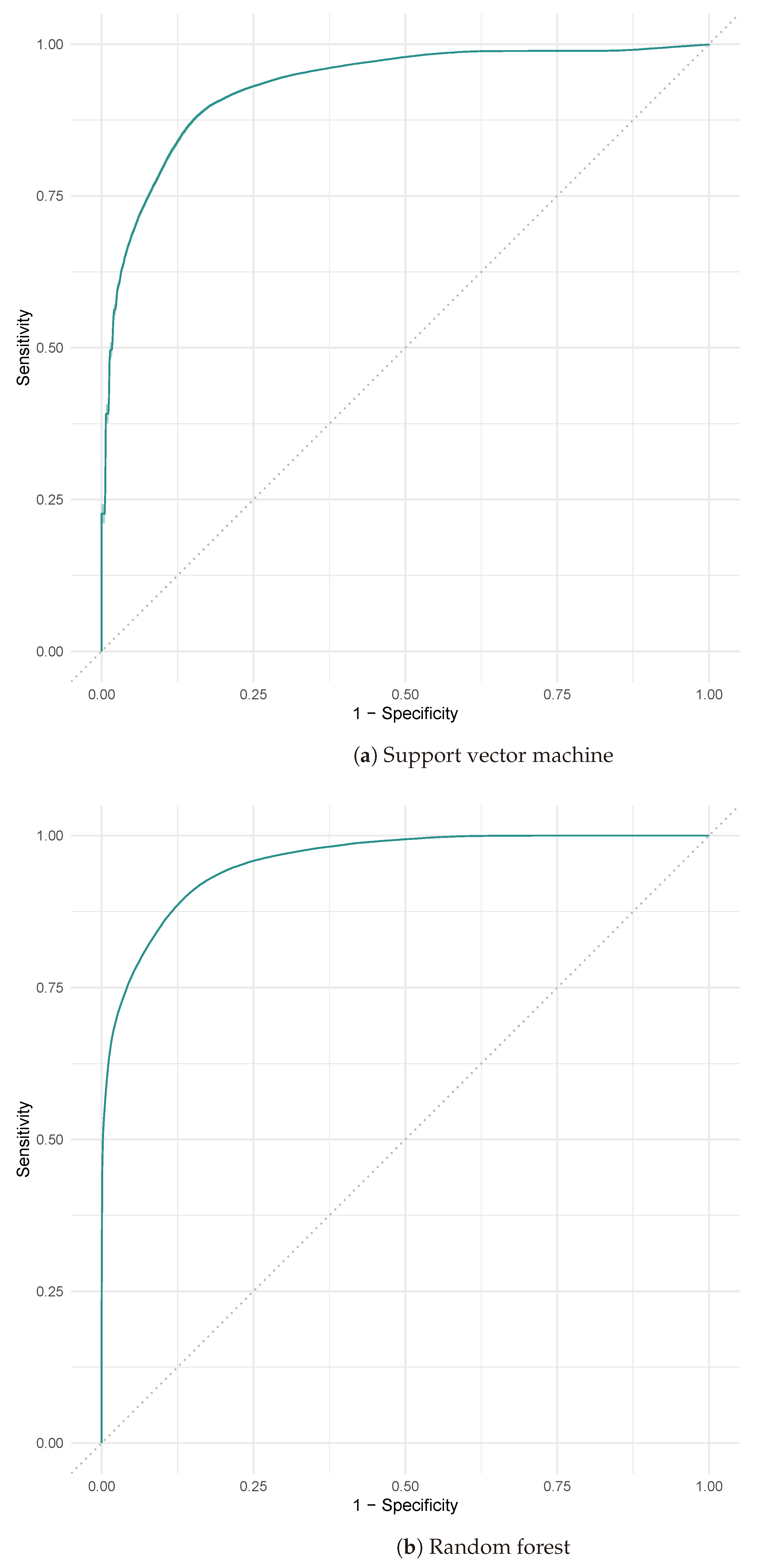
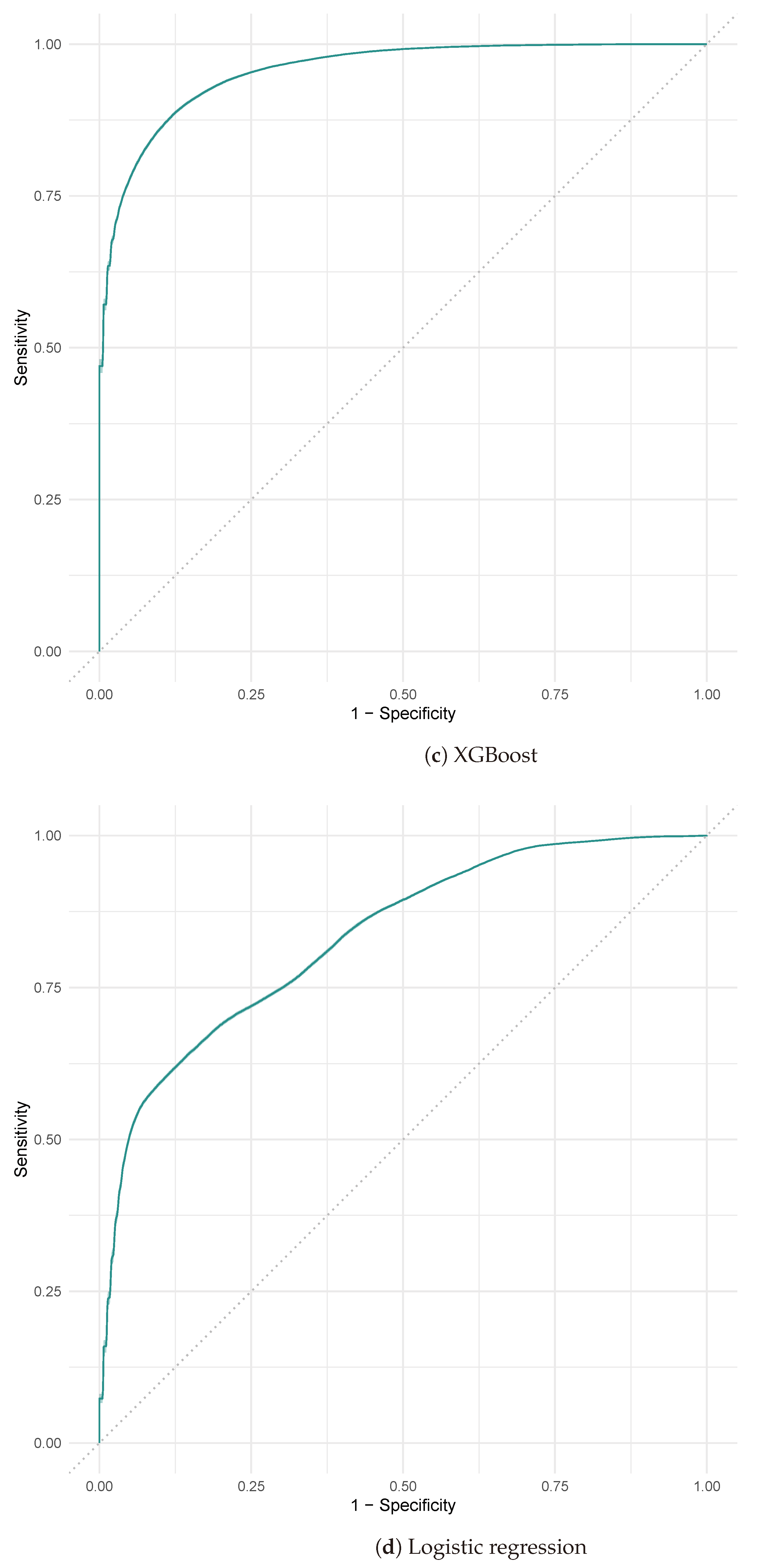
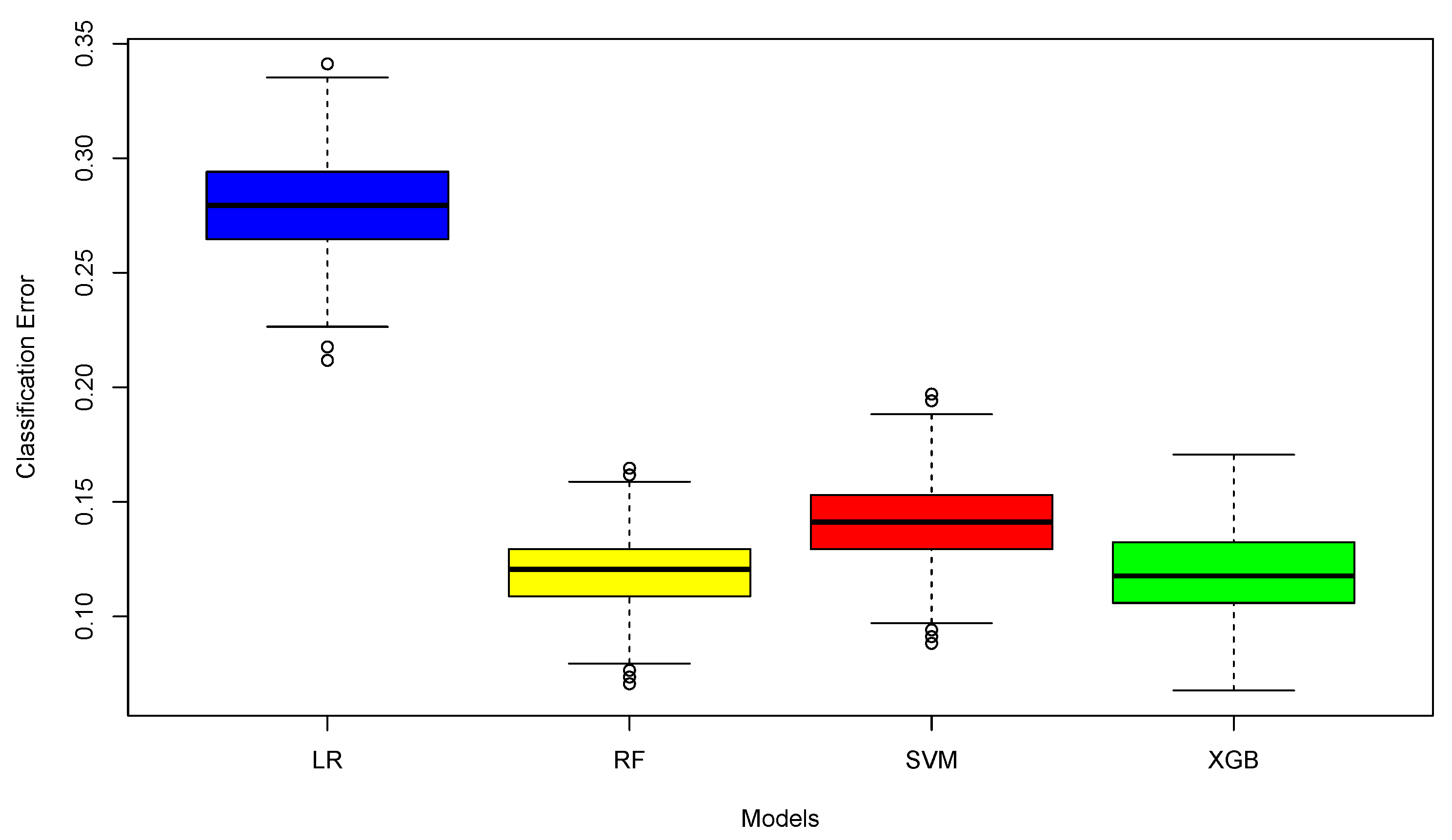
This research addresses this issue by evaluating and comparing four machine learning techniques. In general, RF outperforms the other models in terms of classification effectiveness. In terms of hyperparameter calibration, the available computational resources have been used to perform a grid search. In the case of RF and XGBoost, these algorithms need to adjust a larger set of parameters.

The machine learning models are suitable for solving the studied problem since they are able to handle the complex relationships between LCFs and landslide susceptibility and are robust in noisy environments [88]. The algorithms presented in this paper have been widely used in the literature for the generation of landslide susceptibility maps. SVM has obtained AUROC values ranging from 0.768 to 0.946 ([16,24,88,89,90]). Logistic regression, which is mainly used as a benchmark with which it is possible to make a comparison with other models, has obtained AUROC values ranging from 0.792 to 0.934 ([25,89,90,91,92]). On the other hand, XGBoost, although it has been used in fewer publications than the other algorithms, has obtained promising results: in [93], it obtained an AUROC of 0.96, while in [91], it obtained an AUROC of 0.979. Finally, RF, which almost always achieves excellent results in this problem, has an AUROC ranging from 0.9 to 0.985 ([25,73,89,90,91]), which is consistent with the results obtained and also supported by findings from previous studies ([8,89,94]). One of the advantages that RF has in conjunction with XGBoost is that both are immune to multicollinearity that can occur due to the presence of multiple topographic derivatives as conditioning factors [93], have the ability to handle large data sets, and are resistant to overfitting. Other advantages of RF are that it does not require assumptions on the statistical distribution of the conditioning factors, it takes into account interactions and nonlinear characteristics among the variables, and it has the ability to provide information on the influence of each variable in the final model ([8,25]). The differences between the models lie mainly in the fact that the principles they use to generate predictions are different. SVM is able to map low-dimensional features to high-dimensional spaces using a kernel to find a characteristic hyperplane to maximize the categorical space. The problem with this method is that the corresponding mapping may be poor for the prediction in question, and if the data are noisy or overlapping, the performance of SVM may decrease. RL characterizes the spatial relationship between the landslide events and the conditioning factors, looking for the best-fitting algorithm. However, it is very sensitive to multicollinearity, which limits its performance [90], and also, as the amount of data increases, it may not be able to effectively model the relationship between variables, resulting in a decrease in accuracy. In the case of XGBoost, it can lead to overfitting if the number of trees is not carefully controlled [95].

This study uses a 5-fold cross-validation with 100 replicates in order to calculate the prediction metrics, while most studies use a static data partition to then calculate the indices of interest. This methodology does not deal with the stochastic nature of the problem, so applying cross-validation with repetitions allows us to obtain more robust results. These benefits indicate that it is advisable to continue to use this methodology in future work related to susceptibility assessment.

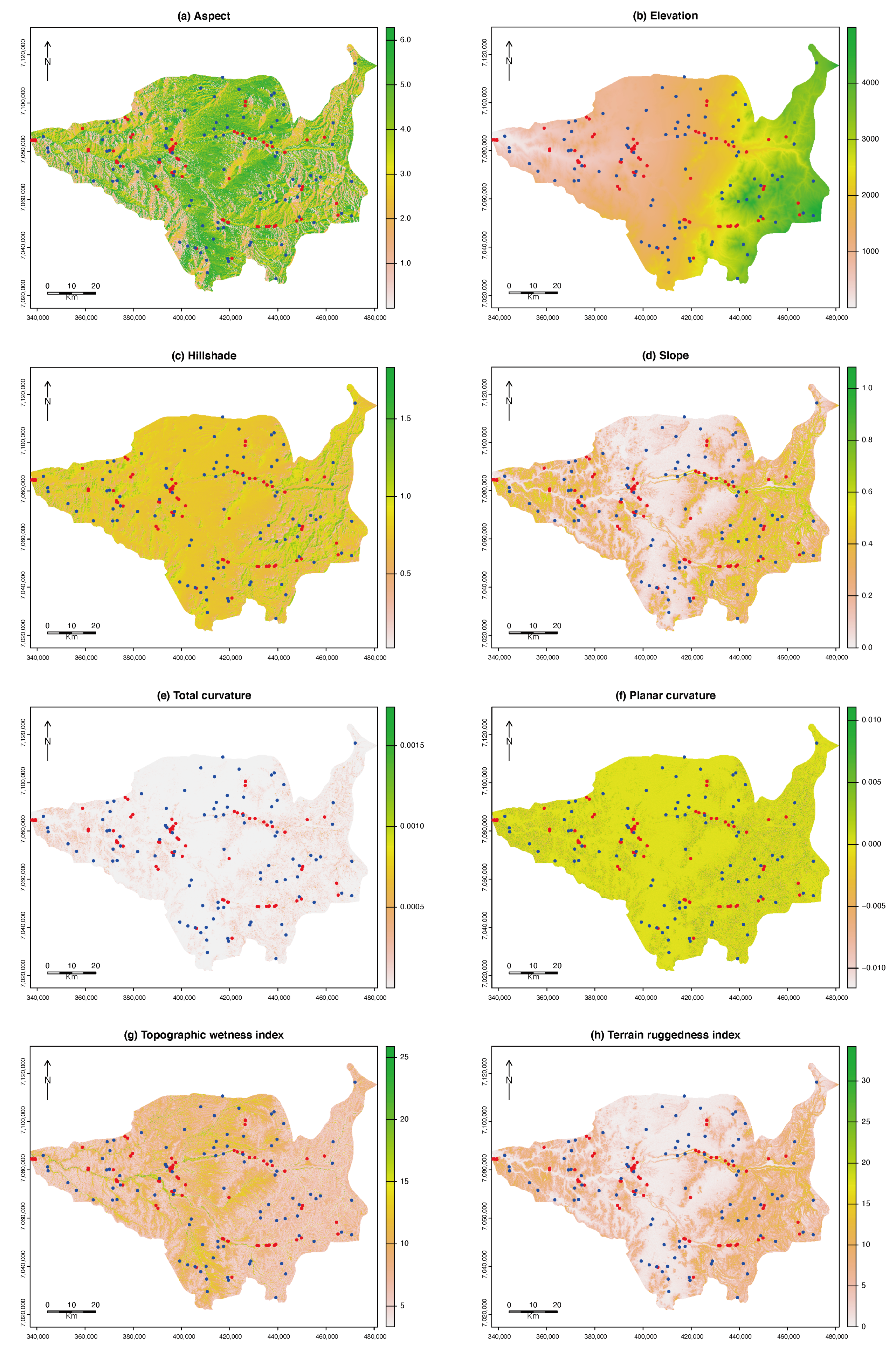
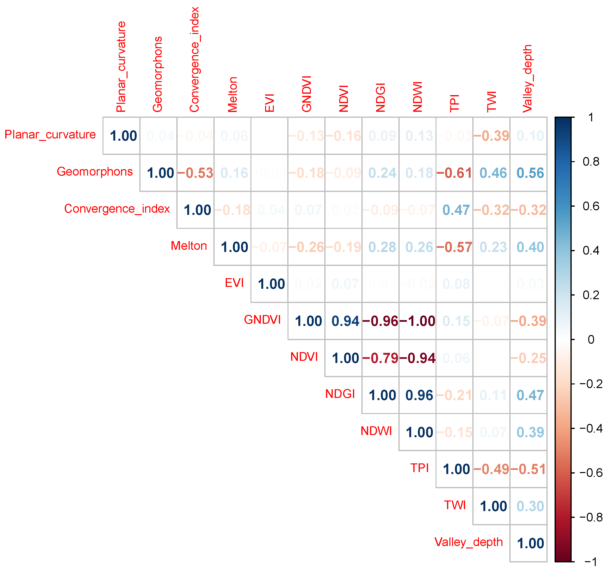
The choice of conditioning factors is a key aspect that influences the quality of susceptibility models [96]. Although various methodologies for selecting factors have been proposed, including linear correlation [31] and the Kolmogorov–Smirnov test [96], there is still no universal criterion for making these selections, and the issue remains a topic for debate [7]. In general, topographic, geologic, soil, hydrologic, geomorphologic, and anthropogenic factors have been accepted in the literature for most susceptibility models. In some cases, factors that do not have predictive capability cause noise, affecting the quality of the model. In addition, it is important to eliminate those factors that have a high correlation index between them to be able to apply cross-validation.

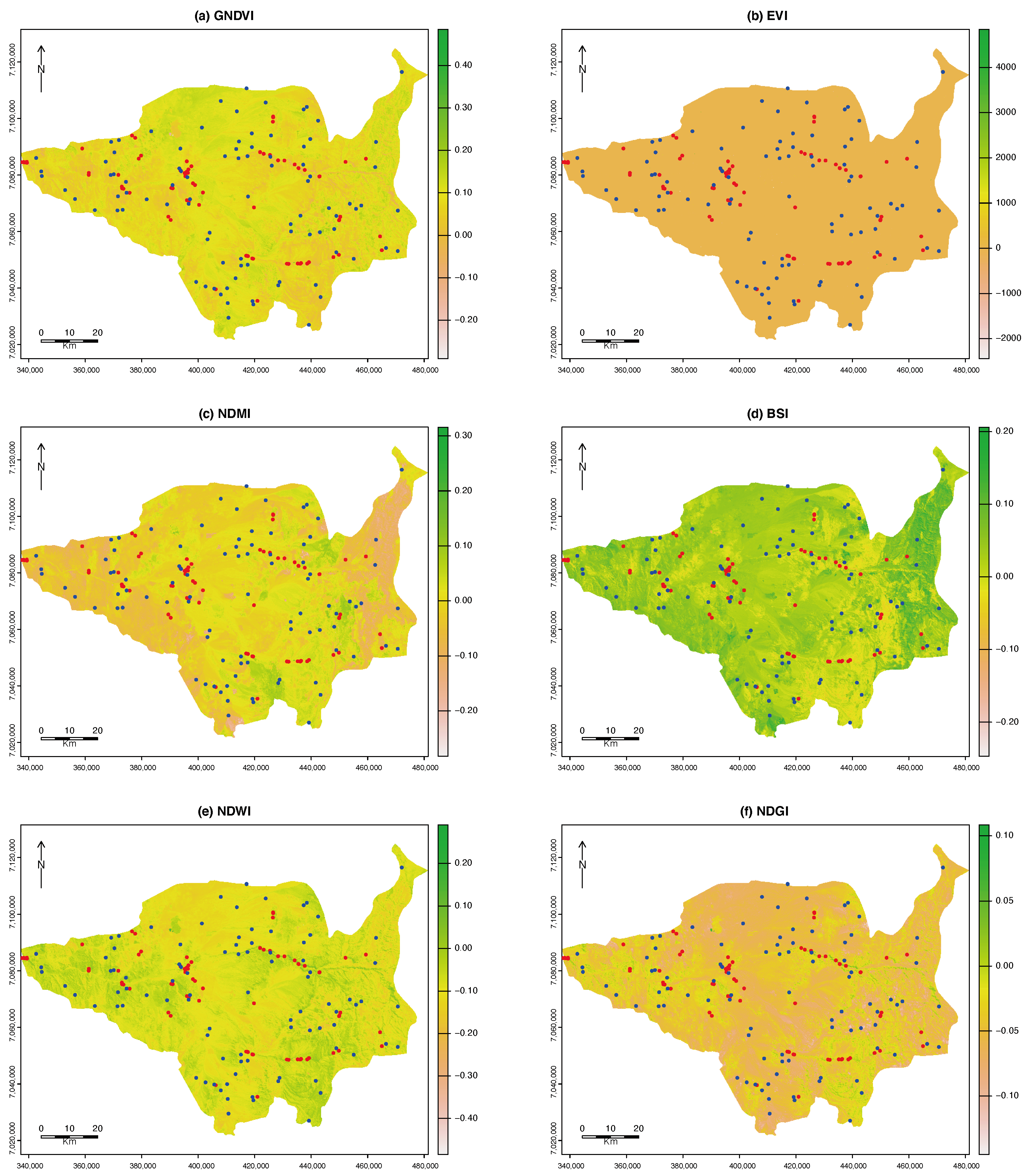
Instead of the widely used NDVI, our model employed the NDGI and EVI spectral indices. This is due to its significant limitations, such as its reliance on the specific time of day when the aerial images are captured, as it does not account for variations in the angle of solar radiation. Hence, this index yields imprecise outcomes. The EVI, calculated in a manner similar to the NDVI, incorporates extra wavelengths to rectify any inaccuracies in the NDVI measurement. This compensates for fluctuations in the solar angle, atmospheric aberrations induced by suspended particles, and land cover indications obscured by vegetation. Furthermore, the EVI may exhibit reduced sensitivity to the soil composition, rendering it more efficient in regions with limited vegetation, where the soil composition can exert a substantial impact on the NDVI. Within our model, the EVI variable exhibits a notable adverse impact, signifying its robust inverse correlation with the incidence of landslides. Higher EVI values suggest that areas with denser and healthier vegetation are less prone to landslides.

On the other hand, the NDGI, primarily utilized for glacier characterization, exhibits a strong predictive capability for susceptibility estimation, as indicated by the IGR. Consequently, it serves as a substitute for the NDVI. In regions with limited vegetation, the NDVI may not be as effective in distinguishing areas that are prone to landslides. On the contrary, the NDGI may be more efficient in semiarid regions or areas with less dense vegetation cover, where it concentrates on particular bands of the spectrum that accurately distinguish between vegetated areas and bare ground or snow. This makes it more suitable for identifying areas prone to landslides. Consequently, regions with sparse vegetation or uncovered soil, which typically exhibit elevated NDGI values in nonglacial settings, are more susceptible to landslides. A high NDGI value may suggest a significant disparity between exposed soil and plant life, potentially indicating regions with limited vegetation coverage. Hence, it is recommended to employ these indices in areas that are analogous to those examined in this study.

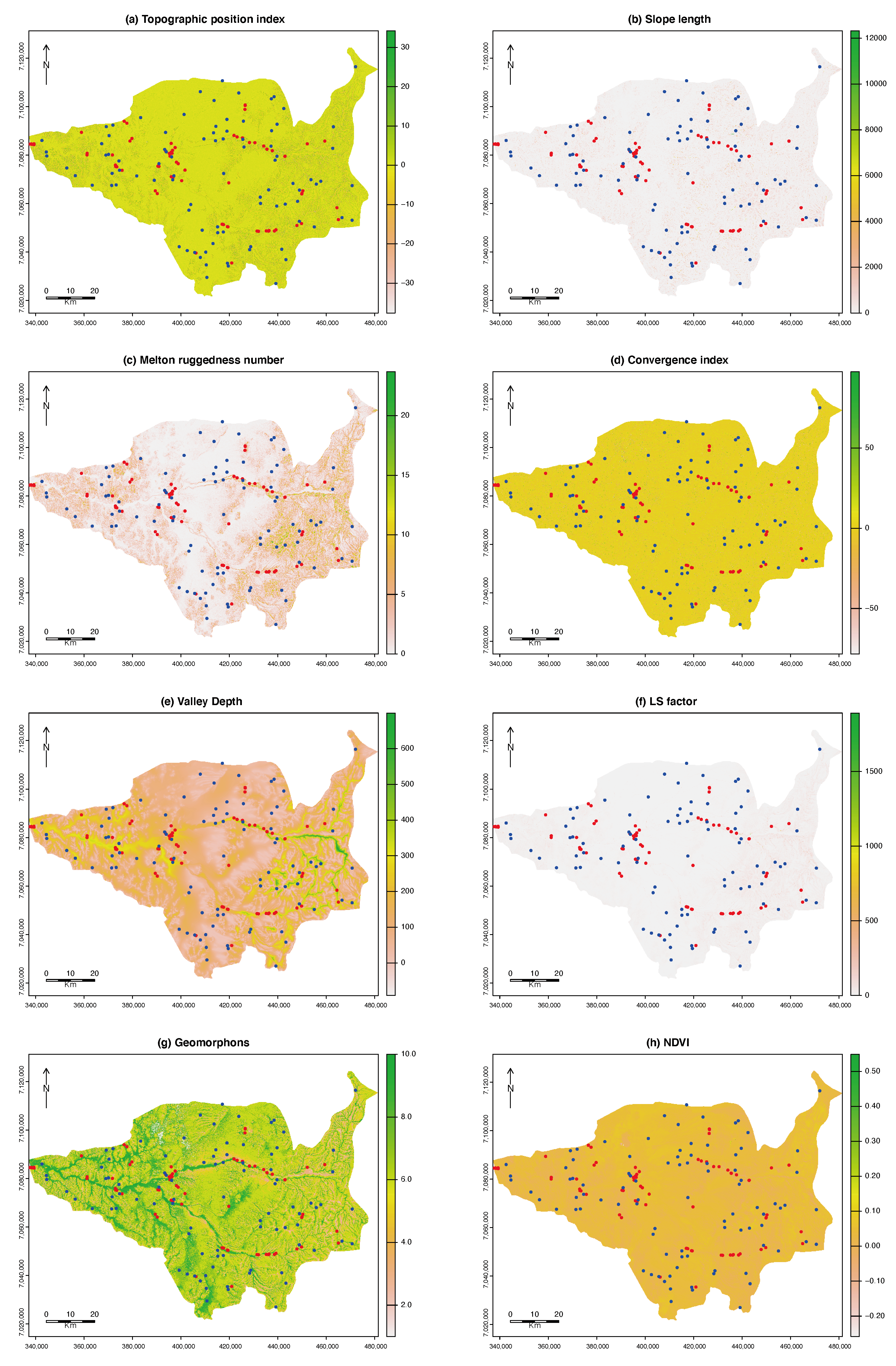
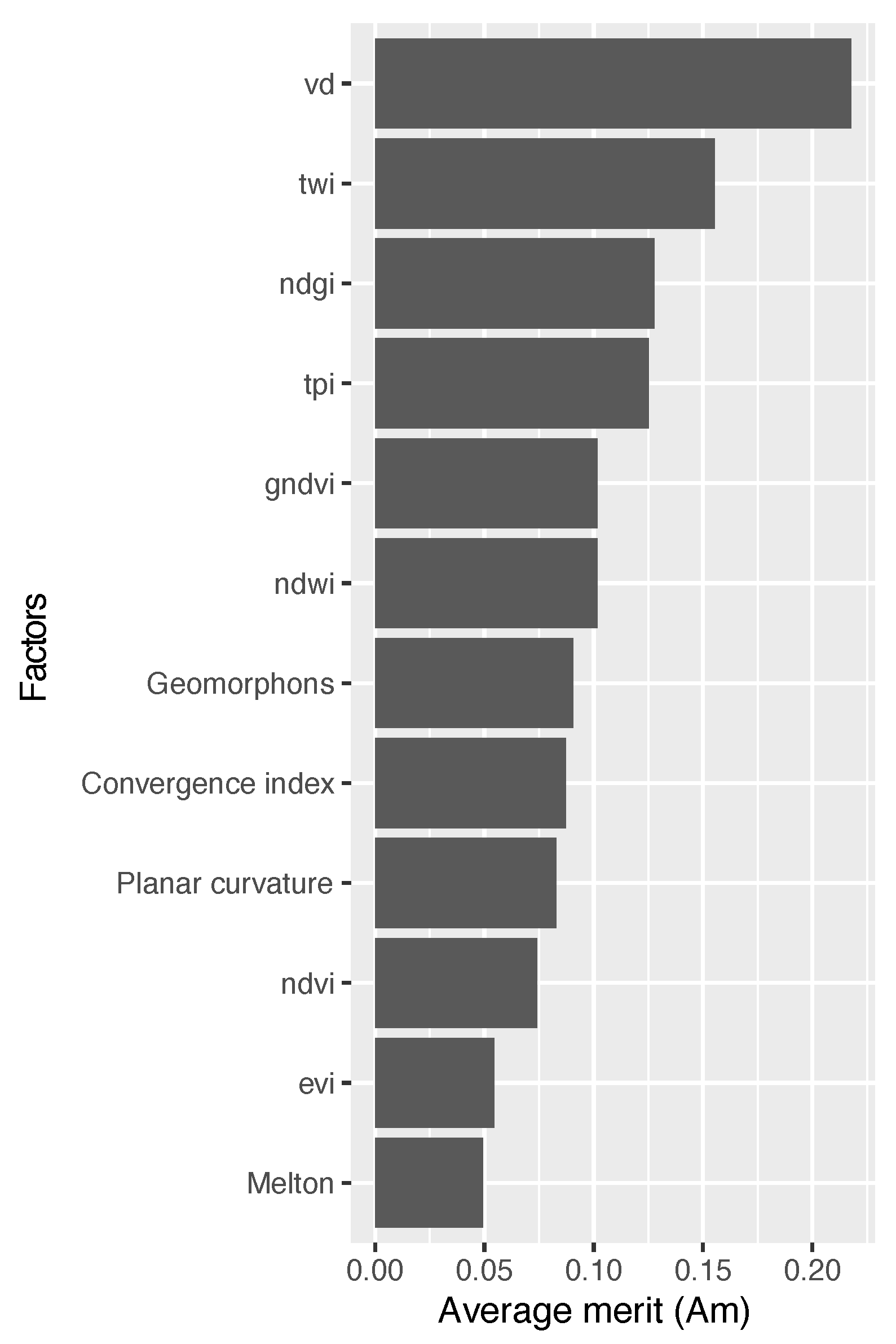
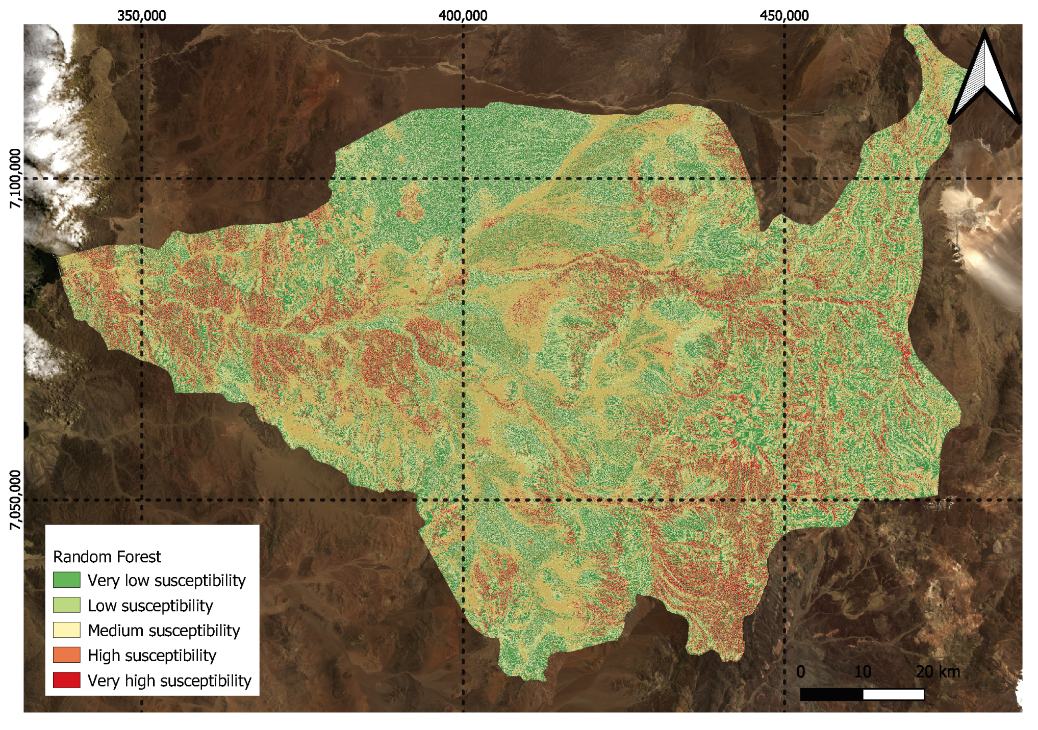
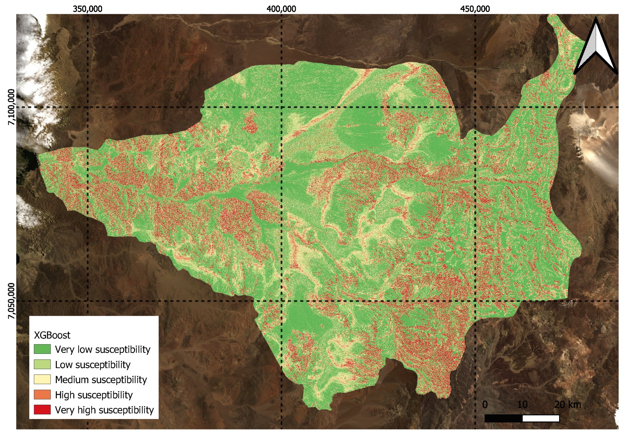
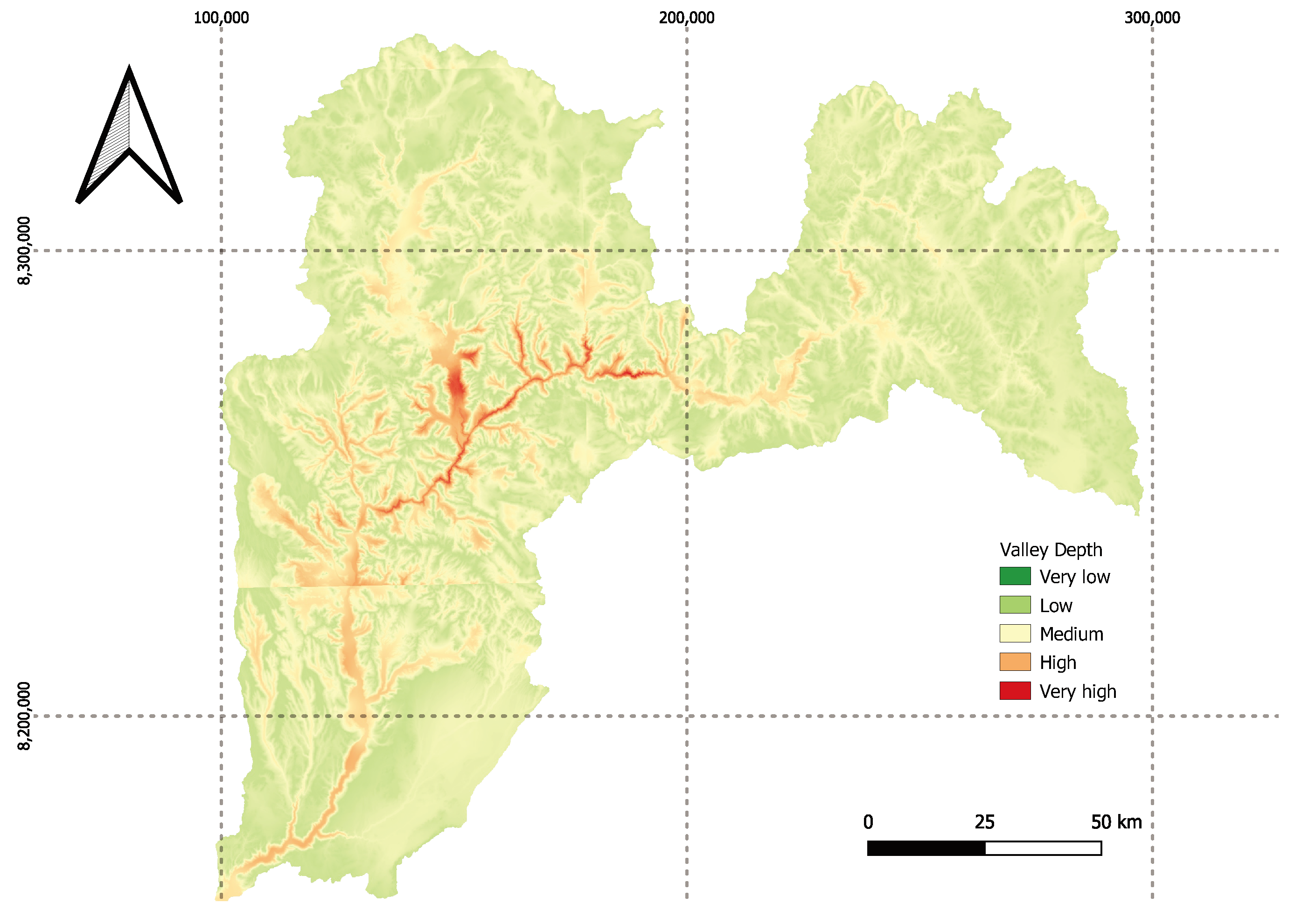
Among the factors studied in this work, two stand out with respect to the others in terms of their influence on the model: the valley depth index (VD) and the TWI. A high valley depth index may be related to a high susceptibility to landslides due to the steep topography and abrupt relief present in the study area, which may favor the occurrence of gravitational processes and increase the erosion rate on the slopes, while a high TWI indicates saturated soil, which implies an increase in the susceptibility to landslides.

It is also novel that the “Valley Depth” (VD) index is the one that provides the most information for the model. The variable VD (valley depth) in the study refers to the vertical distance to the base level of the hydrographic network. This index is calculated using an algorithm that involves interpolating the elevation of the base level of the hydrographic network and then subtracting this base level from the original elevations. This characteristic corresponds to the vertical distance to the base level of the hydrographic network. The algorithm that calculates this index consists of two steps, which involve the interpolation of the elevation of the base level of the hydrographic network and the subsequent subtraction of this base level from the original elevations [97]. A high valley depth index may be related to a high susceptibility to landslides due to the steep topography and abrupt relief present in the study area, which favors the occurrence of gravitational processes and increases the rate of erosion on the slopes. This implies that the landslide and non-landslide sites in the area share similar values of VD, respectively. This aspect is important for morphologies such as that of the Salado River basin, which has a marked slope at the geographic transition as it crosses from the foothills to the intermediate depression and has a “funnel” shape [12].

In summary, the novelty of this study consists of applying repeated cross-validation to obtain the metrics of the models and using the valley depth index, NDGI, and EVI to construct the susceptibility models. Another novelty is the use of the MLR3 package in solving the machine learning problem and the combination with other geospatial packages in R in order to produce the susceptibility maps. Also, the data sources used in the construction of the model proposed in our article come exclusively from satellite images and digital elevation models, unlike other studies, which consider sources of information with a greater number of data and are therefore more difficult for disaster risk management analysts to apply in practice. The method has the advantage in that it can enable the creation of systems that produce susceptibility maps based on the routine updating of satellite images, which can contribute to the development of a susceptibility monitoring system that technical agencies in the disaster area can implement.

After an extensive and updated literature review, we found few publications linked to susceptibility assessment in the Andes. In this regard, we found that in [98], susceptibility mapping was performed in a different Andean area in terms of geomorphology and climate, but like our study, the most successful algorithm corresponds to the random forest. In [99], they use GAM models for the calculation of susceptibility in areas near roads, and here, they note the importance of curvature, like in our study, as an important factor in the calculation of susceptibility. In [100], they also found relevance in the curvature. Finally, in [101], susceptibility maps are used using only the DEM of the zone, holding the results obtained in this work, which also uses satellite imagery. Also, they use a logistic regression model to calculate susceptibility in the Cordillera Blanca, achieving an AUC of 0.75. The region in question presents topographic similarities with the Salado Basin, so the model built in this study may have promising results in that area.

The applicability of the proposed model is determined by the climatic, topographic, and morphometric characteristics of the study area. Under that perspective, the model can be expected to be suitable in areas worldwide that are semiarid zones with a variable topography and a Mediterranean climate with a prolonged dry season, in addition to having narrow and deep valleys where the maximum susceptibility is concentrated. Examples of these zones that are recommended to use this model are the following:

• Colca Valley, Peru: This region is located in southern Peru and has a rugged topography with narrow and deep valleys. The climate is semiarid with a prolonged dry season and has geomorphological characteristics similar to those of the Salado Basin.
• Indo Valley, Pakistan: This valley is located in northern Pakistan and is a mountainous region with deep, narrow valleys. The climate is arid with a prolonged dry season, and the region has a geomorphology similar to the study zone.
• Colorado River Valley, United States: This region is located in the southern part of the state of Colorado and in northern New Mexico. It is a semiarid area with a rugged and mountainous topography and narrow and deep valleys similar to those of the Salado Basin.

To demonstrate the usefulness of the model in other geographical areas, we include a map of the valley depth index in the basin associated with the Colca Valley in Peru (Figure 12), because that factor is the most important in our model. What is interesting about this map is that it is very similar to the generated landslide susceptibility map obtained in [65].

5. Conclusions

This study has comprehensively examined landslide susceptibility in Chañaral province, Chile, using a variety of machine learning algorithms. Our findings reveal a significant influence of topographic and satellite factors, such as the NDGI and EVI, on landslide prediction, bringing a new perspective to the existing literature. We performed a detailed comparison and evaluation of four machine learning models: random forest, support vector machine, XGBoost, and logistic Regression. To train and validate these models, 86 locations were identified as landslides and 86 locations as non-landslides, using 22 conditioning factors, of which 7 were chosen using feature selection techniques such as IGR and Pearson correlation. Furthermore, unlike traditional models, it only uses factors from two easily accessible data sources, which would allow this model to be easily placed in a temporal susceptibility monitoring system in the future.

Model validation was performed through a 5-fold cross-validation repeated 100 times. The metrics employed included the area under the ROC curve (AUC) and classification error to measure the level of accuracy of the models and to determine significant differences between them. The results indicate that the RF and XGBoost models obtain the highest AUC indices, at 0.957 and 0.955, respectively. Furthermore, nonparametric statistical tests indicated that there are no significant statistical differences between them. Maps were generated for these models, highlighting valley depth as the most relevant factor for susceptibility in this area, suggesting its usefulness in similar geographical regions.

The main limitations identified in this work include:

• Integration of other factors: the study focuses only on topographic, hydrological, and satellite factors. Future research could incorporate anthropogenic, geological, or infrastructural factors.
• Spatial resolution: The study area is considerably larger than those commonly analysed in this type of research. It is suggested to limit future studies to a sub-basin of interest and to work with a resolution higher than 30 m/pixel.

These findings offer valuable insights for informed decision making and policy formulation in landslide-prone regions. Overall, our study highlights the potential of machine learning models, especially XGBoost and RF, to accurately and reliably map landslide susceptibility, which is useful for identifying high-risk areas and implementing effective mitigation strategies, benefiting land-use planning authorities and stakeholders. By enhancing the prediction accuracy of landslide susceptibility, we proactively safeguard natural habitats, thereby preserving biodiversity and ecosystem services. Furthermore, the integration of our research into regional sustainability policies can catalyze informed decision making that aligns with sustainable development goals.

References

1. Li, Y.; Liu, X.; Han, Z.; Dou, J. Spatial proximity-based geographically weighted regression model for landslide susceptibility assessment: A case study of Qingchuan area, China. Appl. Sci. 2020, 10, 1107. [Google Scholar] [CrossRef]
2. Wang, Y.; Fang, Z.; Hong, H. Comparison of convolutional neural networks for landslide susceptibility mapping in Yanshan County, China. Sci. Total. Environ. 2019, 666, 975–993. [Google Scholar] [CrossRef]
3. Dang, V.-H.; Hoang, N.-D.; Nguyen, L.-M.-D.; Bui, D.T.; Samui, P. A novel GIS-based random forest machine algorithm for the spatial prediction of shallow landslide susceptibility. Forests 2020, 1, 118. [Google Scholar] [CrossRef]
4. Sun, D.; Wu, X.; Wen, H.; Gu, Q. A LightGBM-based landslide susceptibility model considering the uncertainty of non-landslide samples. Geomat. Nat. Hazards Risk 2023, 14, 2213807. [Google Scholar] [CrossRef]
5. Cao, J.; Zhang, Z.; Wang, C.; Liu, J.; Zhang, L. Susceptibility assessment of landslides triggered by earthquakes in the Western Sichuan Plateau. Catena 2019, 175, 63–76. [Google Scholar] [CrossRef]
6. Saha, S.; Roy, J.; Hembram, T.K.; Pradhan, B.; Dikshit, A.; Abdul Maulud, K.N.; Alamri, A.M. Comparison between deep learning and tree-based machine learning approaches for landslide susceptibility mapping. Water 2021, 13, 2664. [Google Scholar] [CrossRef]
7. Tien Bui, D.; Tuan, T.A.; Klempe, H.; Pradhan, B.; Revhaug, I. Spatial prediction models for shallow landslide hazards: A comparative assessment of the efficacy of support vector machines, artificial neural networks, kernel logistic regression, and logistic model tree. Landslides 2016, 13, 361–378. [Google Scholar] [CrossRef]
8. Pourghasemi, H.R.; Rahmati, O. Prediction of the landslide susceptibility: Which algorithm, which precision? Catena 2018, 162, 177–192. [Google Scholar] [CrossRef]
9. Bui, D.T.; Tsangaratos, P.; Nguyen, V.-T.; Van Liem, N.; Trinh, P.T. Comparing the prediction performance of a Deep Learning Neural Network model with conventional machine learning models in landslide susceptibility assessment. Catena 2020, 188, 104426. [Google Scholar] [CrossRef]
10. Serey, A.; Sepúlveda, S.A.; Murphy, W.; Petley, D.N.; De Pascale, G. Developing conceptual models for the recognition of coseismic landslides hazard for shallow crustal and megathrust earthquakes in different mountain environments—An example from the Chilean Andes. Q. J. Eng. Geol. Hydrogeol. 2021, 54, qjegh2020-023. [Google Scholar] [CrossRef]
11. Marin, M.V.; Muńoz, A.A.; Naranjo, J.A. Víctimas Fatales Causadas por Remociones en Masa en Chile (1928–2017). 2018. Available online: https://www.researchgate.net/profile/Jose-Naranjo-5/publication/329370691_Victimas_fatales_causadas_por_remociones_en_masa_en_Chile_1928-2017/links/5c07b3f0299bf169ae336dda/Victimas-fatales-causadas-por-remociones-en-masa-en-Chile-1928-2017.pdf (accessed on 1 March 2021).
12. González, F. Estudio y ModelacióN 2D del Aluvión de Marzo de 2015 en Chañaral, Atacama; Universidad de Chile: Santiago de Chile, Chile, 2018. [Google Scholar]
13. Vargas Easton, G.; Pérez Tello, S.; Aldunce Ide, P. Aluviones y resiliencia en Atacama. Construyendo saberes sobre riesgos y desastres. In Social Ediciones; Universidad de Chile: Santiago, Chile, 2018. [Google Scholar]
14. Abedini, M.; Ghasemian, B.; Shirzadi, A.; Bui, D.T. A comparative study of support vector machine and logistic model tree classifiers for shallow landslide susceptibility modeling. Environ. Earth Sci. 2019, 78, 560. [Google Scholar] [CrossRef]
15. Luo, W.; Liu, C.C. Innovative landslide susceptibility mapping supported by geomorphon and geographical detector methods. Landslides 2018, 15, 465–474. [Google Scholar] [CrossRef]
16. Abedini, M.; Ghasemian, B.; Shirzadi, A.; Shahabi, H.; Chapi, K.; Pham, B.T.; Bin Ahmad, B.; Tien Bui, D. A novel hybrid approach of bayesian logistic regression and its ensembles for landslide susceptibility assessment. Geocarto Int. 2019, 34, 1427–1457. [Google Scholar] [CrossRef]
17. Merghadi, A.; Yunus, A.P.; Dou, J.; Whiteley, J.; ThaiPham, B.; Bui, D.T.; Avtar, R.; Abderrahmane, B. Machine learning methods for landslide susceptibility studies: A comparative overview of algorithm performance. Earth-Sci. Rev. 2020, 207, 103225. [Google Scholar] [CrossRef]
18. Masek, J.G.; Wulder, M.A.; Markham, B.; McCorkel, J.; Crawford, C.J.; Storey, J.; Jenstrom, D.T. Applicability and performance of deterministic and probabilistic physically based landslide modeling in a data-scarce environment of the Colombian Andes. J. S. Am. Earth Sci. 2021, 108, 103175. [Google Scholar]
19. Elmoulat, M.; Brahim, L.A.; Elmahsani, A.; Abdelouafi, A.; Mastere, M. Mass movements susceptibility mapping by using heuristic approach. Case study: Province of Tétouan (North of Morocco). Geoenviron. Disasters 2021, 8, 20. [Google Scholar] [CrossRef]
20. Zhang, G.; Cai, Y.; Zheng, Z.; Zhen, J.; Liu, Y.; Huang, K. Integration of the statistical index method and the analytic hierarchy process technique for the assessment of landslide susceptibility in Huizhou, China. Catena 2016, 142, 233–244. [Google Scholar] [CrossRef]
21. Regmi, A.D.; Devkota, K.C.; Yoshida, K.; Pradhan, B.; Pourghasemi, H.R.; Kumamoto, T.; Akgun, A. Application of frequency ratio, statistical index, and weights-of-evidence models and their comparison in landslide susceptibility mapping in Central Nepal Himalaya. Arab. J. Geosci. 2014, 7, 725–742. [Google Scholar] [CrossRef]
22. Pham, B.T.; Prakash, I.; Bui, D.T. Spatial prediction of landslides using a hybrid machine learning approach based on random subspace and classification and regression trees. Geomorphology 2018, 303, 256–270. [Google Scholar] [CrossRef]
23. Shirzadi, A.; Saro, L.; Joo, O.H.; Chapi, K. A GIS-based logistic regression model in rock-fall susceptibility mapping along a mountainous road: Salavat Abad case study, Kurdistan, Iran. Nat. Hazards 2012, 64, 1639–1656. [Google Scholar] [CrossRef]
24. Chen, T.; Guestrin, C. Xgboost: A scalable tree boosting system. In Proceedings of the 22nd Acm Sigkdd International Conference on Knowledge Discovery And Data Mining, San Francisco, CA, USA, 13–17 August 2016. [Google Scholar]
25. Tsangaratos, P.; Ilia, I. Landslide susceptibility mapping using a modified decision tree classifier in the Xanthi Perfection, Greece. Landslides 2016, 13, 305–320. [Google Scholar] [CrossRef]
26. Wu, Y.; Ke, Y.; Chen, Z.; Liang, S.; Zhao, H.; Hong, H. Application of alternating decision tree with AdaBoost and bagging ensembles for landslide susceptibility mapping. Catena 2020, 7187, 104396. [Google Scholar] [CrossRef]
27. Hong, H.; Pourghasemi, H.R.; Pourtaghi, Z.S. Landslide susceptibility assessment in Lianhua County (China): A comparison between a random forest data mining technique and bivariate and multivariate statistical models. Geomorphology 2016, 259, 105–118. [Google Scholar] [CrossRef]
28. Wang, Z.; Brenning, A. Active-learning approaches for landslide mapping using support vector machines. Remote Sens. 2021, 13, 2588. [Google Scholar] [CrossRef]
29. Ahmadlou, M.; Karimi, M.; Alizadeh, S.; Shirzadi, A.; Parvinnejhad, D.; Shahabi, H.; Panahi, M. Flood susceptibility assessment using integration of adaptive network-based fuzzy inference system (ANFIS) and biogeography-based optimization (BBO) and BAT algorithms (BA). Geocarto Int. 2020, 34, 1252–1272. [Google Scholar] [CrossRef]
30. Piciullo, L.; Calvello, M.; Cepeda, J.M. Territorial early warning systems for rainfall-induced landslides. Earth-Sci. Rev. 2018, 179, 228–247. [Google Scholar] [CrossRef]
31. Shano, L.; Raghuvanshi, T.K.; Meten, M. Landslide susceptibility evaluation and hazard zonation techniques—A review. Geoenviron. Disasters 2020, 7, 18. [Google Scholar] [CrossRef]
32. Dou, J.; Yunus, A.P.; Xu, Y.; Zhu, Z.; Chen, C.-W.; Sahana, M.; Khosravi, K.; Yang, Y.; Pham, B.T. Torrential rainfall-triggered shallow landslide characteristics and susceptibility assessment using ensemble data-driven models in the Dongjiang Reservoir Watershed, China. Nat. Hazards 2019, 97, 579–609. [Google Scholar] [CrossRef]
33. Ij, H. Statistics versus machine learning. Nat. Methods 2018, 15, 233. [Google Scholar]
34. Lary, D.J.; Alavi, A.H.; Gandomi, A.H.; Walker, A.L. Machine learning in geosciences and remote sensing. Geosci. Front. 2016, 7, 3–10. [Google Scholar] [CrossRef]
35. Miao, F.; Wu, Y.; Xie, Y.; Li, Y. Prediction of landslide displacement with step-like behavior based on multialgorithm optimization and a support vector regression model. Landslides 2018, 15, 475–488. [Google Scholar] [CrossRef]
36. Sekkeravani, M.A.; Bazrafshan, O.; Pourghasemi, H.R.; Holisaz, A. Spatial modeling of land subsidence using machine learning models and statistical methods. Environ. Sci. Pollut. Res. 2022, 29, 28866–28883. [Google Scholar] [CrossRef] [PubMed]
37. Tang, H.; Wang, C.; An, S.; Wang, Q.; Jiang, C. A Novel Heterogeneous Ensemble Framework Based on Machine Learning Models for Shallow Landslide Susceptibility Mapping. Remote Sens. 2023, 15, 4159. [Google Scholar] [CrossRef]
38. Guo, Z.; Shi, Y.; Huang, F.; Fan, X.; Huang, J. Landslide susceptibility zonation method based on C5. 0 decision tree and K-means cluster algorithms to improve the efficiency of risk management. Geosci. Front. 2021, 12, 101249. [Google Scholar] [CrossRef]
39. Mavor, S.P.; Singleton, J.S.; Heuser, G.; Gomila, R.; Seymour, N.M.; Williams, S.; Arancibia, G. Sinistral shear during Middle Jurassic emplacement of the Matancilla Plutonic Complex in northern Chile (25.4° S) as evidence of oblique plate convergence during the early Andean orogeny. J. S. Am. Earth Sci. 2022, 120, 104407. [Google Scholar] [CrossRef]
40. Harrington, H.J. Geology of parts of Antofagasta and Atacama provinces, northern Chile. AAPG Bulletin 1961, 45, 169–197. [Google Scholar]
41. Schulz, N.; Boisier, J.P.; Aceituno, P. Climate change along the arid coast of northern Chile. Int. J. Climatol. 2012, 32, 1803–1814. [Google Scholar] [CrossRef]
42. Tadono, T.; Nagai, H.; Ishida, H.; Oda, F.; Naito, S.; Minakawa, K.; Iwamoto, H. Generation of the 30 M-mesh global digital surface model by ALOS PRISM. Int. Arch. Photogramm. Remote Sens. Spat. Inf. Sci. 2016, 41, 157–162. [Google Scholar] [CrossRef]
43. Masek, J.G.; Wulder, M.A.; Markham, B.; McCorkel, J.; Crawford, C.J.; Storey, J.; Jenstrom, D.T. Landsat 9: Empowering open science and applications through continuity. Remote Sens. Environ. 2020, 248, 111968. [Google Scholar] [CrossRef]
44. Huqqani, I.A.; Tay, L.T.; Mohamad-Saleh, J. Spatial landslide susceptibility modelling using metaheuristic-based machine learning algorithms. Eng. Comput. 2023, 39, 867–891. [Google Scholar] [CrossRef]
45. Ikram RM, A.; Dehrashid, A.A.; Zhang, B.; Chen, Z.; Le, B.N.; Moayedi, H. A novel swarm intelligence: Cuckoo optimization algorithm (COA) and SailFish optimizer (SFO) in landslide susceptibility assessment. Stoch. Environ. Res. Risk Assess. 2023, 37, 1717–1743. [Google Scholar] [CrossRef]
46. Ali, S.A.; Parvin, F.; Pham, Q.B.; Khedher, K.M.; Dehbozorgi, M.; Rabby, Y.W.; Anh, D.T.; Nguyen, D.H. An ensemble random forest tree with SVM, ANN, NBT, and LMT for landslide susceptibility mapping in the Rangit River watershed, India. Nat. Hazards 2022, 113, 1601–1633. [Google Scholar] [CrossRef]
47. Dai, F.C.; Lee, C.F.; Ngai, Y.Y. Landslide risk assessment and management: An overview. Eng. Geol. 2002, 64, 65–87. [Google Scholar] [CrossRef]
48. Alqadhi, S.; Mallick, J.; Talukdar, S.; Bindajam, A.A.; Van Hong, N.; Saha, T. K Selecting optimal conditioning parameters for landslide susceptibility: An experimental research on Aqabat Al-Sulbat, Saudi Arabia. Environ. Sci. Pollut. Res. 2022, 29, 3743–3762. [Google Scholar] [CrossRef] [PubMed]
49. Le Minh, N.; Truyen, P.T.; Van Phong, T.; Jaafari, A.; Amiri, M.; Van Duong, N.; Van Bien, N.; Duc, D.M.; Prakash, I.; Pham, B.T. Ensemble models based on radial basis function network for landslide susceptibility mapping. Environ. Sci. Pollut. Res. 2023, 30, 99380–99398. [Google Scholar] [CrossRef] [PubMed]
50. Qasimi, A.B.; Isazade, V.; Enayat, E.; Nadry, Z.; Majidi, A.H. Landslide susceptibility mapping in Badakhshan province, Afghanistan: A comparative study of machine learning algorithms. Geocarto Int. 2023, 38, 2248082. [Google Scholar] [CrossRef]
51. Nefeslioglu, H.A.; Gokceoglu, C.; Sonmez, H.; Gorum, T. Medium-scale hazard mapping for shallow landslide initiation: The Buyukkoy catchment area (Cayeli, Rize, Turkey). Landslides 2011, 8, 459–483. [Google Scholar] [CrossRef]
52. Chen, W.; Yang, Z. Landslide susceptibility modeling using bivariate statistical-based logistic regression, naïve Bayes, and alternating decision tree models. Bull. Eng. Geol. Environ. 2023, 82, 190. [Google Scholar] [CrossRef]
53. Zhang, Y.; Zhang, J.; Dong, L. Fuzzy Logic Regional Landslide Susceptibility Multi-Field Information Map Representation Analysis Method Constrained by Spatial Characteristics of Mining Factors in Mining Areas. Processes 2023, 11, 985. [Google Scholar] [CrossRef]
54. Kadirhodjaev, A.; Rezaie, F.; Lee, M.J.; Lee, S. Landslide susceptibility assessment using an optimized group method of data handling model. ISPRS Int. J. Geo-Inf. 2020, 9, 566. [Google Scholar] [CrossRef]
55. Kadirhodjaev, A.; Kadavi, P.R.; Lee, C.W.; Lee, S. Analysis of the relationships between topographic factors and landslide occurrence and their application to landslide susceptibility mapping: A case study of Mingchukur, Uzbekistan. Geosci. J. 2018, 22, 1053–1067. [Google Scholar] [CrossRef]
56. Chen, W.; Panahi, M.; Tsangaratos, P.; Shahabi, H.; Ilia, I.; Panahi, S.; Li, S.; Jaafari, A.; Bin Ahmad, B. Applying population-based evolutionary algorithms and a neuro-fuzzy system for modeling landslide susceptibility. Catena 2019, 172, 212–231. [Google Scholar] [CrossRef]
57. Patil, A.S.; Bhadra, B.K.; Panhalkar, S.S.; Patil, P.T. Landslide susceptibility mapping using landslide numerical risk factor model and landslide inventory prepared through OBIA in Chenab Valley, Jammu and Kashmir (India). J. Indian Soc. Remote Sens. 2020, 48, 431–449. [Google Scholar] [CrossRef]
58. Zhong, C.; Oguchi, T.; Lai, R. Effects of Topography on Vegetation Recovery after Shallow Landslides in the Obara and Shobara Districts, Japan. Remote Sens. 2023, 15, 3994. [Google Scholar] [CrossRef]
59. Fatemi Aghda, S.M.; Bagheri, V.; Razifard, M. Landslide susceptibility mapping using fuzzy logic system and its influences on mainlines in lashgarak region, Tehran, Iran. Geotech. Geol. Eng. 2018, 36, 915–937. [Google Scholar] [CrossRef]
60. Rikimaru, A.; Roy, P.S.; Miyatake, S. Tropical forest cover density mapping. Trop. Ecol. 2002, 43, 39–47. [Google Scholar]
61. Benabdelouahab, T.; Balaghi, R.; Hadria, R.; Lionboui, H.; Minet, J.; Tychon, B. Monitoring surface water content using visible and short-wave infrared SPOT-5 data of wheat plots in irrigated semi-arid regions. Int. J. Remote Sens. 2015, 36, 4018–4036. [Google Scholar] [CrossRef]
62. Keshri, A.K.; Shukla, A.; Gupta, R.P. ASTER ratio indices for supraglacial terrain mapping. Int. J. Remote Sens. 2009, 30, 519–524. [Google Scholar] [CrossRef]
63. Es-smairi, A.; Elmoutchou, B.; Mir, R.A.; Touhami AE, O.; Namous, M. Delineation of landslide susceptible zones using Frequency Ratio (FR) and Shannon Entropy (SE) models in northern Rif, Morocco. Geosyst. Geoenviron. 2020, 2, 100195. [Google Scholar] [CrossRef]
64. Nithya, N.S.; Duraiswamy, K. Gain ratio based fuzzy weighted association rule mining classifier for medical diagnostic interface. Sadhana 2014, 39, 39–52. [Google Scholar] [CrossRef]
65. Kumar, C.; Walton, G.; Santi, P.; Luza, C. An Ensemble Approach of Feature Selection and Machine Learning Models for Regional Landslide Susceptibility Mapping in the Arid Mountainous Terrain of Southern Peru. Remote Sens. 2023, 15, 1376. [Google Scholar] [CrossRef]
66. Chapi, K.; Singh, V.P.; Shirzadi, A.; Shahabi, H.; Bui, D.T.; Pham, B.T.; Khosravi, K. A novel hybrid artificial intelligence approach for flood susceptibility assessment. Environ. Model. Softw. 2017, 95, 229–245. [Google Scholar] [CrossRef]
67. Cervantes, J.; Garcia-Lamont, F.; Rodríguez-Mazahua, L.; Lopez, A. A comprehensive survey on support vector machine classification: Applications, challenges and trends. Neurocomputing 2020, 408, 189–215. [Google Scholar] [CrossRef]
68. Kavzoglu, T.; Sahin, E.K.; Colkesen, I. An assessment of multivariate and bivariate approaches in landslide susceptibility mapping: A case study of Duzkoy district. Nat. Hazards 2015, 76, 471–496. [Google Scholar] [CrossRef]
69. Budimir, M.E.A.; Atkinson, P.M.; Lewis, H.G. A systematic review of landslide probability mapping using logistic regression. Landslides 2015, 12, 419–436. [Google Scholar] [CrossRef]
70. Chang, K.-T.; Merghadi, A.; Yunus, A.P.; Pham, B.T.; Dou, J. Evaluating scale effects of topographic variables in landslide susceptibility models using GIS-based machine learning techniques. Sci. Rep. 2019, 9, 12296. [Google Scholar] [CrossRef] [PubMed]
71. Breiman, L. Random forests. Mach. Learn. 2001, 45, 5–32. [Google Scholar]
72. Breiman, L. Classification and Regression Trees; Routledge: New York, NY, USA, 2017. [Google Scholar]
73. Arabameri, A.; Saha, S.; Roy, J.; Chen, W.; Blaschke, T.; Bui, D.T. Landslide susceptibility evaluation and management using different machine learning methods in the Gallicash River Watershed, Iran. Remote Sens. 2020, 12, 475. [Google Scholar] [CrossRef]
74. Gómez-Méndez, I.; Joly, E. Regression with missing data, a comparison study of techniques based on random forests. J. Stat. Comput. Simul. 2023, 1–26. [Google Scholar] [CrossRef]
75. Mienye, I.D.; Sun, Y. A survey of ensemble learning: Concepts, algorithms, applications, and prospects. IEEE Access 2022, 10, 99129–99149. [Google Scholar] [CrossRef]
76. Nielsen, D. Tree Boosting with Xgboost-Why Does Xgboost Win “Every” Machine Learning Competition? Master’s Thesis, NTNU, Trondheim, Norway, 2016. [Google Scholar]
77. Tyralis, H.; Papacharalampous, G. Boosting algorithms in energy research: A systematic review. Neural Comput. Appl. 2021, 33, 14101–14117. [Google Scholar] [CrossRef]
78. Todorov, B.; Billah, A.M. Post-earthquake seismic capacity estimation of reinforced concrete bridge piers using Machine learning techniques. Structures 2022, 41, 1190–1206. [Google Scholar] [CrossRef]
79. Kasraei, B.; Heung, B.; Saurette, D.D.; Schmidt, M.G.; Bulmer, C.E.; Bethel, W. Quantile regression as a generic approach for estimating uncertainty of digital soil maps produced from machine-learning. Environ. Model. Softw. 2021, 144, 105139. [Google Scholar] [CrossRef]
80. Krstajic, D.; Buturovic, L.J.; Leahy, D.E.; Thomas, S. Cross-validation pitfalls when selecting and assessing regression and classification models. J. Cheminfor. 2014, 6, 10. [Google Scholar] [CrossRef] [PubMed]
81. Jonathan, O.; Omoregbe, N.; Misra, S. Empirical comparison of cross-validation and test data on internet traffic classification methods. J. Phys. Conf. Ser. 2019, 1299, 012044. [Google Scholar] [CrossRef]
82. Lovelace, R.; Nowosad, J.; Muenchow, J. Geocomputation with R; Chapman Hall: London, UK; CRC: Boca Raton, FL, USA, 2019. [Google Scholar]
83. Berger, V.W.; Zhou, Y.Y. Kolmogorov–smirnov test: Overview. In Wiley StatsRef: Statistics Reference Online; Wiley: Hoboken, NJ, USA, 2014. [Google Scholar]
84. Ostertagova, E.; Ostertag, O.; Kováč, J. Methodology and application of the Kruskal-Wallis test. Appl. Mech. Mater. 2014, 611, 115–120. [Google Scholar] [CrossRef]
85. Liu, Y.; Chen, W. A SAS macro for testing differences among three or more independent groups using Kruskal-Wallis and Nemenyi tests. J. Huazhong Univ. Sci. Technol. [Med. Sci.] 2012, 32, 130–134. [Google Scholar] [CrossRef]
86. Lang, M.; Binder, M.; Richter, J.; Schratz, P.; Pfisterer, F.; Coors, S.; Au, Q.; Casalicchio, G.; Kotthoff, L.; Bischl, B. mlr3: A modern object-oriented machine learning framework in R. J. Open Source Softw. 2019, 4, 1903. [Google Scholar] [CrossRef]
87. Aguirre-Gutiérrez, J.; Carvalheiro, L.G.; Polce, C.; van Loon, E.E.; Raes, N.; Reemer, M.; Biesmeijer, J.C. Fit-for-purpose: Species distribution model performance depends on evaluation criteria—Dutch hoverflies as a case study. PLoS ONE 2013, 8, e63708. [Google Scholar] [CrossRef]
88. Huang, F.; Cao, Z.; Guo, J.; Jiang, S.H.; Li, S.; Guo, Z. Comparisons of heuristic, general statistical and machine learning models for landslide susceptibility prediction and mapping. Catena 2020, 191, 104580. [Google Scholar] [CrossRef]
89. Zhao, P.; Masoumi, Z.; Kalantari, M.; Aflaki, M.; Mansourian, A. A GIS-Based Landslide Susceptibility Mapping and Variable Importance Analysis Using Artificial Intelligent Training-Based Methods. Remote Sens. 2022, 14, 211. [Google Scholar] [CrossRef]
90. Huang, F.; Cao, Z.; Guo, J.; Jiang, S.H.; Li, S.; Guo, Z. The uncertainty of landslide susceptibility prediction modeling: Suitability of linear conditioning factors. Bull. Eng. Geol. Environ. 2022, 81, 182. [Google Scholar] [CrossRef]
91. Bruzón, A.G.; Arrogante-Funes, P.; Arrogante-Funes, F.; Martín-González, F.; Novillo, C.J.; Fernández, R.R.; Ramos-Bernal, R.N. Landslide susceptibility assessment using an AutoML. framework Int. J. Environ. Res. Public Health 2021, 18, 10971. [Google Scholar] [CrossRef] [PubMed]
92. Zhu, L.; Huang, L.; Fan, L.; Huang, J.; Huang, F.; Chen, J.; Wang, Y. Landslide susceptibility prediction modeling based on remote sensing and a novel deep learning algorithm of a cascade-parallel recurrent neural network. Sensors 2020, 20, 1576. [Google Scholar] [CrossRef] [PubMed]
93. Can, R.; Kocaman, S.; Gokceoglu, C. A comprehensive assessment of XGBoost algorithm for landslide susceptibility mapping in the upper basin of Ataturk dam, Turkey. Appl. Sci. 2020, 11, 4993. [Google Scholar] [CrossRef]
94. Ali, S.A.; Parvin, F.; Vojteková, J.; Costache, R.; Linh, N.T.T.; Pham, Q.B.; Ghorbani, M.A. GIS-based landslide susceptibility modeling: A comparison between fuzzy multi-criteria and machine learning algorithms. Geosci. Front. 2021, 12, 857–876. [Google Scholar] [CrossRef]
95. Abedi, R.; Costache, R.; Shafizadeh-Moghadam, H.; Pham, Q.B. Flash-flood susceptibility mapping based on XGBoost, random forest and boosted regression trees. Geocarto Int. 2022, 37, 5479–5496. [Google Scholar] [CrossRef]
96. Costanzo, D.; Chacón, J.; Conoscenti, C.; Irigaray, C.; Rotigliano, E. Forward logistic regression for earth-flow landslide susceptibility assessment in the Platani river basin (southern Sicily, Italy). Landslides 2014, 11, 639–653. [Google Scholar] [CrossRef]
97. Conrad, O.; Bechtel, B.; Bock, M.; Dietrich, H.; Fischer, E.; Gerlitz, L.; Wehberg, J.; Wichmann, V.; Böhner, J. System for automated geoscientific analyses (SAGA) v. 2.1.4. Geosci. Model Dev. 2015, 8, 1991–2007. [Google Scholar] [CrossRef]
98. Ospina-Gutiérrez, J.P.; Aristizábal, E. Aplicación de inteligencia artificial y técnicas de aprendizaje automático para la evaluación de la susceptibilidad por movimientos en masa. Rev. Mex. Cienc. Geológicas 2021, 38, 43–54. [Google Scholar] [CrossRef]
99. Brenning, A.; Schwinn, M.; Ruiz-Páez, A.P.; Muenchow, J. Landslide susceptibility near highways is increased by 1 order of magnitude in the Andes of southern Ecuador, Loja province. Nat. Hazards Earth Syst. Sci. 2015, 15, 45–57. [Google Scholar] [CrossRef]
100. Lizama, E.; Morales, B.; Somos-Valenzuela, M.; Chen, N.; Liu, M. Understanding landslide susceptibility in Northern Chilean Patagonia: A basin-scale study using machine learning and field data. Appl. Sci. 2022, 14, 907. [Google Scholar] [CrossRef]
101. Bueechi, E.; Klimeš, J.; Frey, H.; Huggel, C.; Strozzi, T.; Cochachin, A. Regional-scale landslide susceptibility modelling in the Cordillera Blanca, Peru—A comparison of different approaches. Landslides 2019, 16, 395–407. [Google Scholar] [CrossRef]
Figure 1. Map of the study area.
Sustainability 15 16806 g001
Figure 2. Thematic maps—1. (a) aspect; (b) Elevation; (c) hillshade; (d) slope; (e) total curvature; (f) planar curvature; (g) topographic wetness index (TWI); (h) terrain ruggedness index (TRI).
Sustainability 15 16806 g002
Figure 3. Thematic maps—2. (a) Topographic position index; (b) slope; (c) Melton ruggedness number; (d) convergence index; (e) valley depth; (f) LS factor; (g) geomorphons; (h) NDVI.
Sustainability 15 16806 g003
Figure 4. Thematic maps—3. (a) GNDVI; (b) EVI; (c) NDMI; (d) BSI; (e) NDWI; (f) NDGI.
Sustainability 15 16806 g004
Figure 5. Experimental model.
Sustainability 15 16806 g005
Figure 6. Predictive power of factors according to IGR.
Sustainability 15 16806 g006
Figure 7. Summary chart—correlation.
Sustainability 15 16806 g007
Figure 8. ROC curves after cross-validation. Test set. The x-axis corresponds to 1 s p e c i f i t y and the y-axis is the s e n s i t i v i t y . (a) SVM; (b) random forest; (c) XGBoost; (d) logistic regression.
Sustainability 15 16806 g008aSustainability 15 16806 g008b
Figure 9. Comparison of classification error values for the different models.
Sustainability 15 16806 g009
Figure 10. Susceptibility map—RF.
Sustainability 15 16806 g010
Figure 11. Susceptibility map—XGBoost.
Sustainability 15 16806 g011
Figure 12. Valley depth index map in Colca Valley, Perú. EPSG 32718.
Sustainability 15 16806 g012