Effects of Topography on Vegetation Recovery after Shallow Landslides in the Obara and Shobara Districts, Japan

Abstract

Intense rainfall-induced shallow landslides can have severe consequences, including soil erosion and vegetation loss, making in-depth research essential for disaster risk management. However, vegetation recovery processes after shallow landslides and their influencing multivariate factors are not well known. This study aims to address this gap by investigating the vegetation recovery processes after shallow landslides and the impact of topography on this recovery. We focus on two regions in Japan: the Shobara district in Hiroshima Prefecture and the Obara district in Aichi Prefecture. The Normalized Difference Vegetation Index (NDVI) and Enhanced Vegetation Index (EVI) derived from long-term Landsat images, as well as aerial photographs and environmental datasets, are used to measure vegetation recovery. Then, statistical analysis and the Seasonal Autoregressive Integrated Moving Averages (SARIMA) model were employed to investigate the dynamic response of vegetation under different combinations of environmental conditions using NDVI and EVI time series. Historical aerial photographs and vegetation index trend analysis suggest that vegetation in the study areas will take more than ten years to return to a stable state. The results also demonstrate the influence of atmospheric and land cover conditions when monitoring vegetation response using NDVI and EVI. In Obara, concave and convergent terrain positively influenced NDVI, while non-steep, low-elevation, and north-facing terrain positively influenced EVI. In Shobara, gentle and northwest-facing slopes were positively correlated with NDVI, and gentle and west-facing slopes were positively correlated with EVI. SARIMA modeling found that NDVI is more suitable for modeling the middle and late stages of vegetation recovery within 10–25 years after the landslide. In comparison, EVI is better for modeling the early stage of vegetation recovery within 10 years after the landslide.

1. Introduction

Rainfall-induced landslides can have severe consequences on communities [1]. Japan is prone to rainfall-induced landslides due to its geological, geomorphological, and climatic conditions [2]. Examining vegetation recovery following shallow landslides can offer valuable insights into improving future disaster recovery efforts.

Recent advances in Geographic Information Systems (GIS) and remote sensing technology have enabled researchers to collect detailed information to monitor vegetation recovery over space and time [3,4,5,6]. Vegetation indices are commonly used to extract data from multiple spectral bands to investigate vegetation changes [7,8,9,10,11]. These indices usually rely on the measurement of greenness using algebraic combinations between different spectral bands, particularly the red and near-infrared (NIR) bands [12,13]. The Normalized Difference Vegetation Index (NDVI) [14] and Enhanced Vegetation Index (EVI) [15], which are derived from NIR-based spectral indices, are frequently used to monitor vegetation recovery. The NDVI is chlorophyll sensitive, whereas the EVI is more responsive to canopy structural variations [16]. Li et al. (2010) compared and evaluated the accuracy of predicting natural vegetation cover using NDVI and EVI based on the Moderate Resolution Imaging Spectroradiometer (MODIS) sensor by developing optimal regression equations for grassland, shrub, and forest samples. They found that NDVI has apparent advantages for predicting natural vegetation coverage over EVI [17]. Matsushita et al. (2007) presented a theoretical analysis of the topographic effect on EVI and NDVI using a non-Lambertian model. In a case study utilizing airborne-based images from a mountainous area with a dense Japanese cypress plantation, they found that EVI is more sensitive to topographic conditions than NDVI [18]. However, the comparative applicability and performance of NDVI and EVI in monitoring and simulating dynamic vegetation recovery in mountainous forest areas under various environmental conditions are still poorly understood. Thus, identifying appropriate and interpretable vegetation indices is necessary to comprehend vegetation responses after landslides under different environmental conditions.

The effectiveness of vegetation indices in representing vegetation recovery is heavily influenced by the type of landscape disturbance, soil characteristics, and topography [19]. For example, aspect is a crucial control of an area’s microclimate, localized hydrological variability, and soil hydrophobicity [20]. The slope gradient is critical in controlling soil moisture and affecting growing vegetation [21]. One or more topographic variables can significantly change the vegetation index response, and indices have different sensitivities to environmental conditions [22]. Vegetation also affects geomorphic processes through precipitation–vegetation–erosion feedback [23,24,25]. Considering the interdependence between topography and vegetation is crucial for effective vegetation recovery monitoring. Several studies have analyzed the suitability and relevance of different vegetation indices, considering several confounding factors, notably topographic variables, for vegetation monitoring [26,27,28].

Recent improvements in remote sensing technology and enhanced computing capabilities have provided researchers with unprecedented access to data, leading to a better comprehension of large-scale vegetation recovery over extended periods. These advances have created novel opportunities to investigate the complex connection between topography and vegetation recovery over time. Therefore, this study examines topography’s influence on vegetation recovery in landslide-affected areas in two study areas, the Shobara district in Hiroshima Prefecture and the Obara district in Aichi Prefecture, Japan. These areas were selected based on their susceptibility to shallow landslides owing to geological conditions and the availability of Landsat satellite images, aerial photographs of vegetation conditions, and environmental variables datasets. The study comprises four key components to achieve its objective. Firstly, we used historical aerial photographs to identify areas impacted by landslides. Secondly, we assessed vegetation recovery using vegetation indices derived from long-term satellite imagery. Thirdly, we analyzed correlations and time series data to evaluate the relationship between vegetation recovery and environmental variables. Finally, we compared the effectiveness of different vegetation indices for monitoring vegetation recovery under varying ecological conditions.

2. Materials and Methods

2.1. Study Areas

2.1.1. Obara District

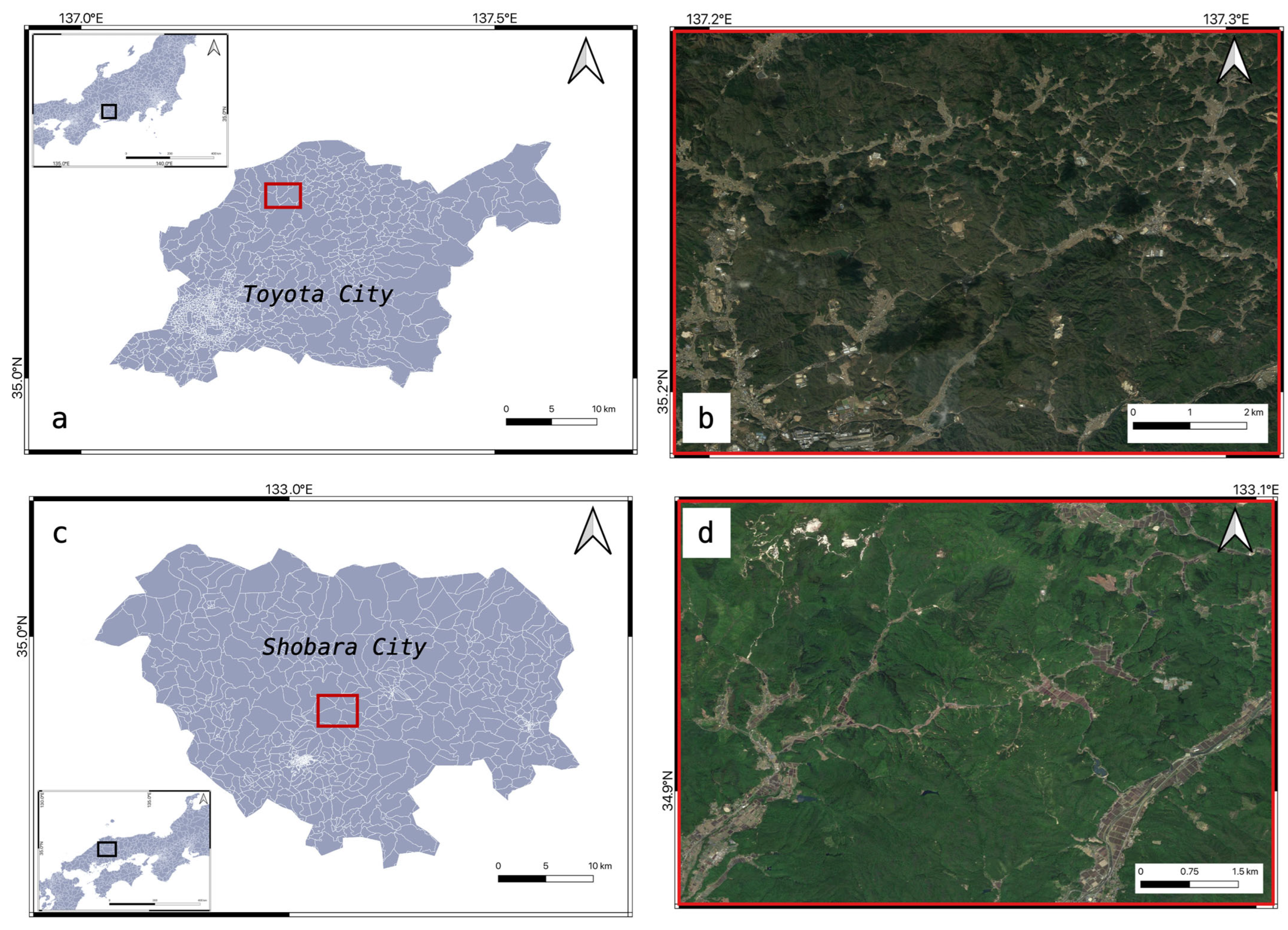
The first study area is the Obara district in Toyota City, northern Aichi Prefecture, central Japan (Figure 1a,b). The region’s topography consists of low-relief mountains with elevations ranging from 200 to 600 m. This area experienced heavy rainfall on 12–13 July 1972, with precipitation of 218 mm per 5 h, resulting in numerous shallow landslides [29]. The affected areas consist mainly of weathered granitoid, making the area prone to shallow landslides [30]. The two main types of granitoid in the study area are coarse-grained granite (CG) and medium-grained granite (MG) [31]. Vegetation is scarce on cliffs, and the other areas are mainly covered with red spruce trees [32]. The subsequent post-landslide vegetation recovery process is natural.

2.1.2. Shobara District

The Shobara district is in Shobara City, in northeastern Hiroshima Prefecture of western Japan (Figure 1c,d). On 16 July 2010, a severe rainstorm caused over a thousand shallow landslides [33]. The region’s geology primarily comprises rhyolite (RL) and andesite (AS). The topography is characterized by low-relief mountains, with elevations ranging from 250 to 650 m. Deciduous broad-leaved forests cover most slopes, with some areas consisting of conifer forests [34].

2.2. Data

2.2.1. Aerial Photographs

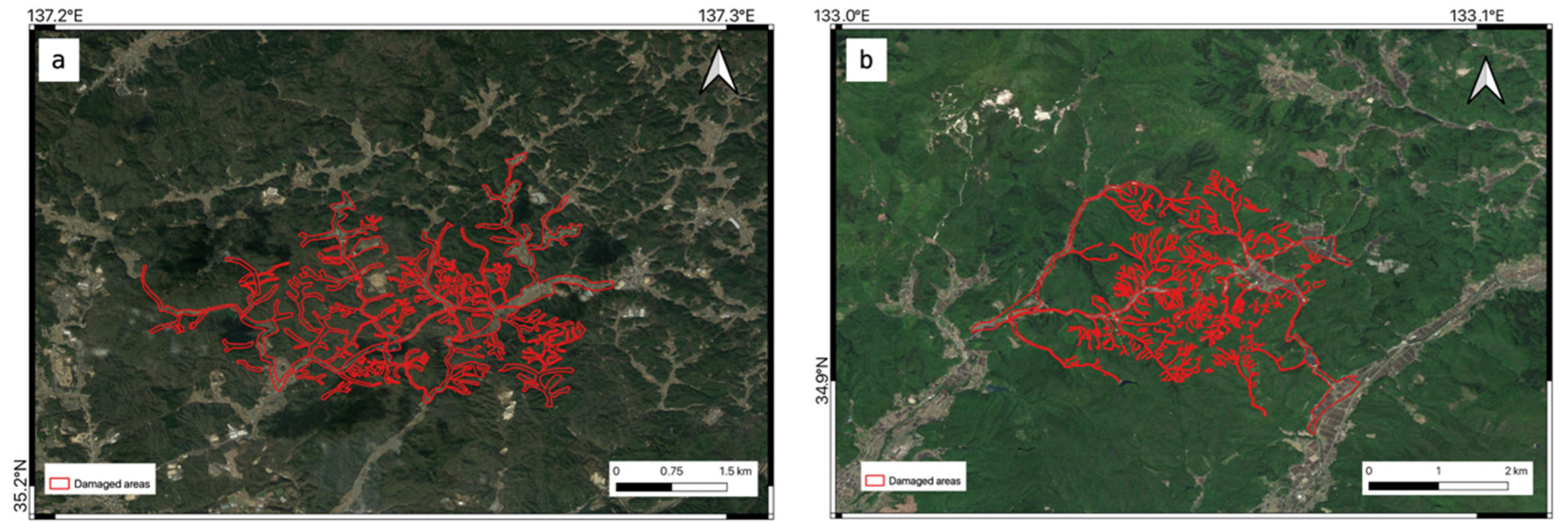
Historical aerial photographs were obtained from the Geospatial Information Authority of Japan for different years: 1968, 1972, 1974, 1977, 1982, 1998, and 2000 for the Obara district and 1975 and 2010 for the Shobara district. We compared the pre- and post-landslide conditions of the study areas to create maps by visual inspection to show the distribution of damaged areas affected by the landslides (Figure 2). While areas with known human activities were excluded during the extraction of damaged areas, it should be acknowledged that some areas may have been affected by human activities, such as conversion to farmland, during the subsequent recovery period. However, the proportion of affected pixels in both study areas is less than 1%, rendering their impact insignificant for our analysis.

2.2.2. Satellite Imagery

Long-term time series satellite data were used to investigate the vegetation recovery processes. For Obara, Landsat 5 surface reflectance spanning 28 years (January 1984 to May 2012) with 30 m resolution was obtained from the National Aeronautics and Space Administration (NASA). Satellite imagery before 1984 was unavailable for Obara due to significant coverage gaps in Landsat 1–3 Multispectral Scanner (MSS) data. Furthermore, the absence of a blue band in Landsat 1–3 MSS hindered the calculation of EVI. For Shobara, Landsat 7 and 8 surface reflectance data were acquired at 30 m resolution over 22 years (January 1999 to November 2021) and eight years (April 2013 to December 2021), respectively. We then conducted other processing steps on the Landsat time series through Google Earth Engine (GEE), a cloud-computing platform capable of handling satellite imagery and geospatial datasets [35].

2.2.3. Geological Type Database

We obtained a geological distribution map from the geological map display system of the Geological Survey of Japan to investigate the impact of geological type on vegetation recovery. We generated a vector shapefile layer using the map to represent the geological conditions of various regions in the two study areas. This geological layer was co-registered with satellite imagery to analyze the correlation between geological type and vegetation recovery.

2.2.4. Digital Elevation Models

Digital elevation models (DEMs) were obtained from NASA’s Shuttle Radar Topography Mission (SRTM) digital elevation 30 m and used in GEE to calculate various topographic variables (

Table 1. Summary of topographic variables used for statistical analysis. The value ranges are those of data from the sources mentioned above.

Topographic Variables	Unit	Description	Value Range
			Obara	Shobara
Elevation (E)	m	Height of terrain above sea level	0–330	90–500
Slope gradient (S)	degrees	Slope gradient	0–80	0–80
Aspect (A)	degrees	Compass direction	0–360	0–360
Horizontal curvature (HC)	m	Curvature tangent to the contour line	−0.1–0.2	−0.1–0.2
Vertical curvature (VC)	m	Curvature tangent to the slope line	−0.01–0.04	−0.1–0.1
Maximal curvature (MC)	m	Highest values of curvature	−0.01–0.2	−0.01–0.3

). The consistent spatial resolution with Landsat imagery enabled direct comparison of calculated variables to Landsat data. These variables were selected based on their known impact on vegetation growth and survival. Elevation affects temperature and moisture, creating climatic gradients as elevation changes [36]. Slope gradient affects land stability and erosion rates and has been shown to impact vegetation recovery in eroded rills and gullies [21]. Aspect, the direction of a slope, creates spatial differences in solar insolation that can influence hydrologic, ecological, and geomorphic processes [20]. Additionally, curvature, divided into horizontal curvature, vertical curvature, and maximal curvature, is a crucial factor affecting soil moisture distribution and water transport, ultimately affecting vegetation growth [37].

3. Method

The methodology used in this study consists of three main stages: preprocessing of the satellite image time series, computation of vegetation recovery trends on a pixel-by-pixel basis, and identification of significant variables via statistical analysis to be utilized in subsequent time series analysis.

3.1. Preprocessing Landsat Time Series

We applied various filtering and processing techniques to preprocess the reflectance dataset acquired from Landsat 5, 7, and 8 satellite imagery. We used the damaged areas distribution map extracted from the pre- and post-landslide aerial photographs to constrain the Landsat data to the boundary of the damaged areas. The Landsat surface reflectance images have already been calibrated, converted to top-of-atmosphere reflectance, and atmospherically corrected [38] to ensure high quality images suitable for time series analysis. Data with less than 80% cloud cover over land and geometric root mean squared error of less than 10% were filtered, and terrain correction was applied to minimize topographic shading. Given the smaller size of the study areas compared to the Landsat footprint and the acquisition of multiple satellite images per month or year, an 80% cloud cover filter is unlikely to significantly impact the data extracted from study areas because image composition was performed per month or year. After terrain correction, the images were harmonized [39], classified by year and month, and then composited separately yearly and monthly, resulting in datasets of yearly and monthly median multispectral images. Annual values were employed to assess long-term trends and changes in vegetation conditions. Monthly values were used to evaluate seasonal trends in vegetation conditions.

3.2. Computing Vegetation Indices and Deriving Recovery Trends

This study analyzed vegetation recovery in landslide areas using two commonly used vegetation indices, the Normalized Difference Vegetation Index (NDVI) and the Enhanced Vegetation Index (EVI). EVI is preferred for its improved vegetation monitoring capability [40]. On the other hand, NDVI is chosen because it provides reliable vegetation cover estimates across various vegetation types [41] and different soil and lithological backgrounds [42]. Its ability to normalize minimizes the effect of background variations [43]. Furthermore, NDVI is frequently preferred for long-term observations compared to the Soil Adjusted Vegetation Indices (SAVI), which are more suitable for sparsely vegetated areas [44]. Although NDVI has drawbacks such as topographic illumination and shading effects issues [18,45], terrain correction during the preprocessing of Landsat time series data can generally address these limitations caused by the topographic relief [46]. To calculate average annual vegetation index values after rainfall-induced landslides, the study period was set from 1985 to 2011 for Obara and from 2011 to 2020 for Shobara. The study periods were chosen to ensure complete data coverage during the summer months of each year (June, July, and August), thus providing an accurate representation of the annual vegetation index. Annual NDVI and EVI values were obtained using linear regression for Obara time series data and log-linear regression for Shobara, reflecting the distinct vegetation recovery patterns in each study area. These regression methods were chosen based on approaches used in previous studies [47,48] to provide a simplified representation of the vegetation recovery patterns observed in each study area.

NDVI is calculated as

$$NDVI=\frac{NIR-RED}{NIR+RED}$$

(1)

where NIR is the near-infrared band intensity and RED is the red band intensity.

EVI corrects for some atmospheric conditions and canopy background noise [15]. It is calculated as

$$EVI=2.5\times \frac{(NIR-RED)}{(NIR+6RED-7.5BLUE+1)}$$

(2)

where BLUE is the blue band intensity, the value of 2.5 represents the gain factor, 6 and 7.5 represent the coefficients of the aerosol resistance term, and adding the value of 1 adjusts the canopy background [49]. All parameters were defined according to the Landsat EVI description from USGS [50].

The differences in $d_{NDVI}$ and $d_{EVI}$ calculated from two images after landslides were used to assess the net change in vegetation index value for vegetation change distribution calculation and further statistical analysis:

$$d_{NDVI}={NDVI}_{year2}-{NDVI}_{year1}$$

(3)

$$d_{EVI}={EVI}_{year2}-{EVI}_{year1}$$

(4)

In this study, $year1$ and $year2$ represent the start and end years of the study period for each area. We used linear regression for Obara and log-linear regression for Shobara to determine the values of ${NDVI}_{year1}$, ${NDVI}_{year2}$, ${EVI}_{year1}$, and ${EVI}_{year2}$. These regression models were applied to the NDVI and EVI time series data, enabling us to derive the indicators for the start and end years of the study period.

3.3. Statistical Analysis

To investigate the relationship between environmental variables and vegetation recovery, locations of damaged areas, Landsat time series, and topographic variables were converted into a vector shapefile layer and georeferenced to the EPSG:4326 coordinate system using GEE. Then, we performed multivariate analysis, including analysis of variance (ANOVA) and Tukey Honestly Significant Difference (Tukey HSD) tests. One-way, two-way, and three-way ANOVAs were conducted to understand environmental variables’ effects on vegetation recovery comprehensively. One-way ANOVA reflects the impact of each environmental variable on vegetation recovery. Two-way ANOVA shows the combined effects of two environmental variables and their interactions. Three-way ANOVA allows us to investigate the simultaneous effects of three environmental variables and their interactions. In addition, Tukey HSD [51] analysis was conducted following ANOVA to understand which specific groups of environmental variables differ by determining the honest significant differences between group means. Furthermore, Spearman’s correlation coefficient [52] was employed to assess the positive or negative relationships between the identified significantly different groups and vegetation indices.

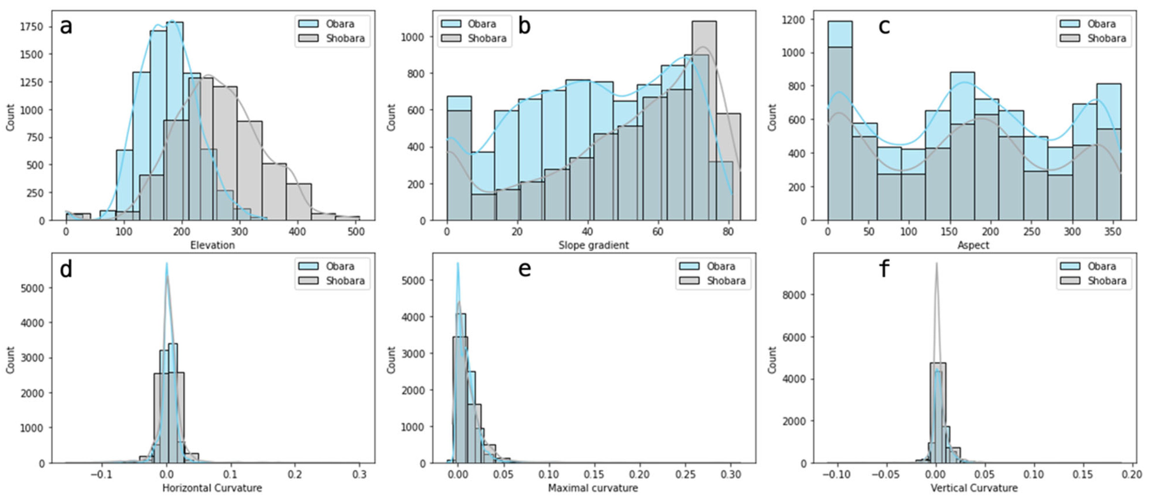
Categorizing the data for conducting ANOVA is necessary to determine if there are statistically significant differences between the categories. The categories presented in

Table 2. Summary of environmental variables’ categories used for statistical analysis.

Topographic Variables		Categories
Obara	Shobara
E (m)
0–80	90–190	Lower level
80–160	190–290	Lower-middle level
160–240	290–390	Upper-middle level
240–330	390–500	Upper level
S (degrees)
0–20	0–20	Gentler slopes
20–40	20–40	Gentler-moderate slopes
40–60	40–60	Steeper-moderate slopes
60–80	60–80	Steeper slopes
A (degrees)
0–45	0–45	N
45–90	45–90	NE
90–135	90–135	E
135–180	135–180	SE
180–225	180–225	S
225–270	225–270	SW
270–315	270–315	W
315–360	315–360	NW
HC (m)
−0.1–0	−0.1–0	Convergent terrain
0–0.1	0–0.1	Slightly divergent terrain
0.1–0.2	0.1–0.2	Divergent terrain
VC (m)
−0.01–0	−0.1–0	Concave terrain
0–0.02	0–0.02	Slightly convex terrain
0.02–0.04	0.02–0.1	Convex terrain
MC (m)
−0.01–0	−0.01–0	Convergent and concave terrain
0–0.1	0–0.1	Slightly divergent and convex terrain
0.1–0.2	0.1–0.3	Divergent and convex terrain
G
CG	RL	-
MG	AS	-

were defined based on the range of values observed in the data (Figure 3), with varying bin widths chosen to suit the data distribution. Elevation, slope gradient, and aspect were divided into several groups based on the range of values. Horizontal, vertical, and maximal curvature were split into three groups centered around zero and boundary values. Geology (G) was categorized based on geological type. These groups were considered as independent variables, while $d_{NDVI}$ and $d_{EVI}$ were dependent variables. A p-value of less than 0.01 was used to determine statistical significance.

3.4. Modeling Vegetation Recovery

The vegetation response was modeled using the Seasonal Autoregressive Integrated Moving Averages (SARIMA) Box–Jenkins model [53]. A comparative analysis of NDVI and EVI responses and modeling performance was conducted under different environmental conditions in the two study cases. Specifically, we considered Shobara as a case representing the early stage of vegetation recovery, while Obara represented the middle and late stages.

The SARIMA model helps model stochastic processes considering the past behavior of a time series. It can be composed of an autoregressive (AR) model, a moving average (MA) model, or a combination of both (ARMA). The ARMA model is appropriate for stationary series where values vary uniformly around the mean without trend. However, for non-stationary series, such as those represented by the vegetation indices in this study, it is necessary to achieve stationarity by identifying and removing all factors contributing to non-stationarity, resulting in an Autoregressive Integrated Moving Averages (ARIMA) model. Moreover, vegetation index time series often exhibit marked seasonality, which can be incorporated into the Seasonal ARIMA (SARIMA) model through seasonal differences. The SARIMA model is represented as

SARIMA(p,d,q)(P,D,Q)_S

(5)

where p and q are the orders of the AR and MA models, respectively, and d is the order of the difference applied to the series to achieve stationarity. P, D, and Q are the orders of the seasonal differences used concerning a seasonal period S [54]. The simplified equation for the SARIMA model is

$${\varphi }_p\left(B\right){\Phi }_p\left(B^S\right){\nabla }^d{\nabla }_S^D{Y}_t={\theta }_q\left(B\right){\Theta }_Q\left(B^S\right){\epsilon }_t$$

(6)

where $Y_t$ is the observed value of the time series in period t with a seasonal period of S, ${\epsilon }_t$ is a white noise process in period t, and $B$ is a simple or seasonal backshift operator where for each ${\epsilon }_t$: $B{\epsilon }_t={\epsilon }_{t-1}$ and $B^S{\epsilon }_t={\epsilon }_{t-S}$. In this way, the operators of the simple, seasonal AR and MA models can be written concerning B. Furthermore, the $\nabla$ operator of the simple and seasonal differences is also written in terms of B for each ${\epsilon }_t$.

Building a SARIMA model involves three main steps: identification, parameter training and test number estimation, and model assessment. In the identification step, the orders of differencing d and D were selected to achieve stationarity, and the order of the autoregressive (AR), moving average (MA), and seasonal components (P and Q) of the model were determined based on the analysis of autocorrelation functions (ACFs) and partial autocorrelation functions (PACFs) of the differenced series. After the identification step, we estimated all parameters in Equation (5) and the number of training and test data points. Three statistical indices were used to evaluate the model performance: the determination coefficient (R²), the Mean Absolute Percentage Error (MAPE), and the Root Mean Square Error (RMSE). The best model was selected based on the highest overall performance for each time series. Furthermore, we evaluated the performance of the best model to determine the vegetation indices suitable for modeling vegetation recovery trends under different environmental conditions in the two study cases.

4. Results

4.1. NDVI and EVI Responses to Vegetation Recovery

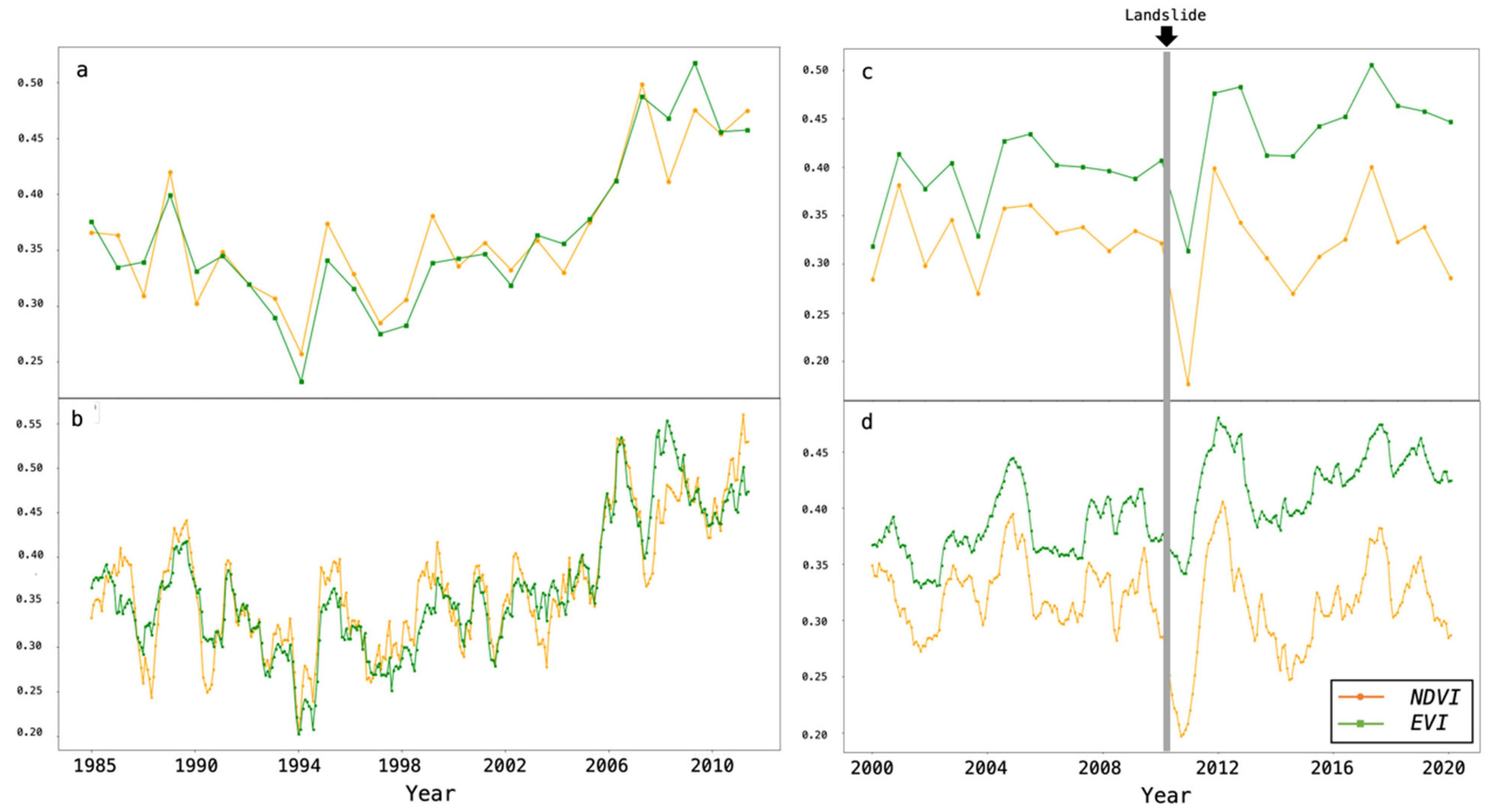
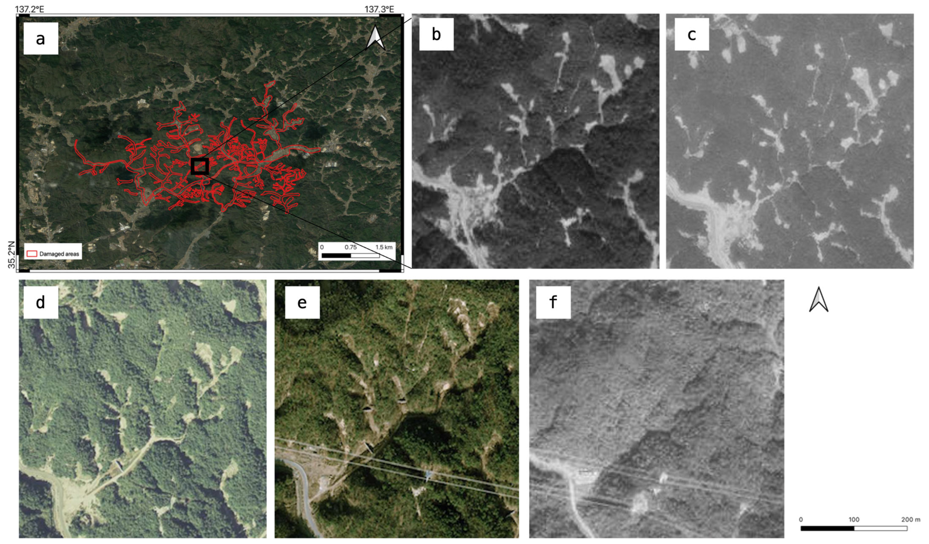
The temporal changes in NDVI and EVI exhibit a distinct seasonal pattern. High NDVI and EVI characterize the summer season from July to October, while lower NDVI and EVI were observed during the withering season from December to April (Figure 4b,d). There is a negligible difference between NDVI and EVI temporal changes in both study areas and seasonal cycles. The annual mean NDVI and EVI on the damaged slopes ranged from 0.2 to 0.6 in the Obara district (Figure 4a). In Shobara, the mean annual NDVI and EVI in the damaged areas ranged from 0.1 to 0.6 (Figure 4c). Before the heavy rainfall in 2011, the NDVI values at Shobara ranged from 0.25 to 0.45. However, in 2011, a year after the rainfall-induced landslide event, the mean NDVI and EVI decreased to 0.2 and 0.3, respectively (Figure 4c). For Obara, although satellite imagery was unavailable before 1985, the increasing trend in annual mean NDVI and EVI between 1985 and 2011 indicates continuous recovery even after landslides occurred approximately ten years earlier (Figure 4a). Aerial photographs showed rainfall-induced landslides in Obara caused vegetation loss in July 1972 (Figure 5b). Post-rainfall aerial photographs from 1972 to 1998 showed increased vegetation coverage in the damaged areas over the years, suggesting vegetation recovery (Figure 5b–f).

The regression models used to derive ${NDVI}_{year1}$, ${NDVI}_{year2}$, ${EVI}_{year1}$, and ${EVI}_{year2}$ for $d_{NDVI}$ and $d_{EVI}$ calculations demonstrated the following best fits: linear regression in Obara (NDVI: R² = 0.36; EVI: R² = 0.38) and log-linear regression in Shobara (NDVI: R² = 0.14; EVI: R² = 0. 34). Changes in vegetation indices were categorized using the threshold values of $d_{NDVI}$ and $d_{EVI}$, as described in

Table 3. Threshold values of $d_{NDVI}$ and $d_{EVI}$ and the corresponding frequency distribution in the Obara district and the Shobara district. “Poor” to “Excellent” categories indicate increasing positive changes in vegetation index values. “Very poor” means a negative change in the vegetation index value.

Category	Obara			Shobara
	$d_{NDVI}$ and $d_{EVI}$	$\mathrm{Distribution} (\%) \mathrm{of} d_{NDVI}$	$\mathrm{Distribution} (\%) \mathrm{of} d_{EVI}$	$d_{NDVI}$ and $d_{EVI}$	$\mathrm{Distribution} (\%) \mathrm{of} d_{NDVI}$	$\mathrm{Distribution} (\%) \mathrm{of} d_{EVI}$
Excellent	>0.3	33.8	5.1	>0.2	18.6	1.9
Very good	0.2–0.3	28.1	6.9	0.1–0.2	39.4	12.2
Good	0.1–0.2	21.3	37.8	0.05–0.1	22.9	19.9
Poor	0–0.1	16.4	31.8	0–0.05	19.1	29.3
Very poor	<0	0.4	18.4	<0	0	36.7

. The same threshold values for $d_{NDVI}$ and $d_{EVI}$ were used for each area to compare the differences in NDVI and EVI changes over time after landslides. Overall, $d_{NDVI}$ exhibited greater changes than $d_{EVI}$ in both study areas.

4.2. Statistical Analyses on Environmental Variables Influencing Vegetation Recovery

The results of the one-way ANOVA analysis (

Table 4. Statistical analysis results of one-way ANOVA.

Variable	Obara		Shobara
	$d_{NDVI}$	$d_{EVI}$	$d_{NDVI}$	$d_{EVI}$
E	0.18	0.05	0.02	0.06
S	0.02	0.03	0.02	0.02
A	0.03	0.02	0.01 *	0.009 *
HC	0.002 *	0.06	0.07	0.19
VC	0.049	0.003 *	0.085	0.271
MC	0.05	0.003 *	0.044	0.128
G	0.005 *	0.02	0.07	0.14

* indicates statistical significance equal to or lower than 1%.

) reveal that in Obara, horizontal curvature and geological type significantly affect $d_{NDVI}$, whereas vertical curvature and maximum curvature affect $d_{EVI}$. In contrast, in Shobara, the aspect significantly affects both $d_{NDVI}$ and $d_{EVI}$. The two-way ANOVA results (

Table 5. Statistical analysis results of two-way ANOVA.

Variable1	Variable2	Obara		Shobara
		$d_{NDVI}$	$d_{EVI}$	$d_{NDVI}$	$d_{EVI}$
E	S	0.1	0.1	0.139	0.1
	A	0.001 *	0.006 *	0.028	0.559
	HC	0.089	0.017	0.084	0.076
	VC	0.001 *	0.001 *	0.075	0.001 *
	MC	0.045	0.001 *	0.01 *	0.071
	G	0.023	0.2	0.078	0.34
S	A	0.001 *	0.1	0.01 *	0.006 *
	HC	0.081	0.001 *	0.103	0.766
	VC	0.104	0.301	0.01 *	0.001 *
	MC	0.503	0.143	0.023	0.607
	G	0.100	0.100	0.56	0.67
A	HC	0.309	0.592	0.305	0.107
	VC	0.11	0.022	0.337	0.09
	MC	0.001 *	0.001 *	0.003 *	0.640
	G	0.02	0.05	0.56	0.41
HC	VC	0.488	0.107	0.65	0.572
	MC	0.100	0.200	0.01 *	0.021
	G	0.146	0.166	0.27	0.34
VC	MC	0.002 *	0.236	0.2	0.276
	G	0.2	0.14	0.1	0.1
MC	G	0.18	0.20	0.5	0.67

* indicates statistical significance equal to or lower than 1%.

) indicate that in Obara, the combination of maximum curvature or aspect with elevation, slope gradient, and vertical curvature significantly affects both $d_{NDVI}$ and $d_{EVI}$. Similarly, in Shobara, the combination of maximum curvature or aspect with elevation, slope gradient, and vertical curvature significantly affects $d_{NDVI}$ and $d_{EVI}$. Interestingly, the aspect effect is significant in vegetation recovery from one-way and two-way ANOVA. Furthermore, geological type does not show effective results in the two-way ANOVA analysis in either study area, indicating its independence from other topographic variables. The three-way ANOVA analysis (

Table 6. Statistical analysis results of three-way ANOVA.

Variable1	Variable2	Variable3	Obara		Shobara
			$d_{NDVI}$	$d_{EVI}$	$d_{NDVI}$	$d_{EVI}$
E	S	A	0.005 *	0.001 *	0.001 *	0.005 *
		HC	0.01 *	0.001 *	0.007 *	0.057
		VC	0.01 *	0.001 *	0.068	0.018
		MC	0.001 *	0.001 *	0.685	0.117
		G	0.278	0.346	0.510	0.690
S	A	HC	0.01 *	0.003 *	0.019	0.02
		VC	0.007 *	0.001 *	0.004 *	0.002
		MC	0.001 *	0.001 *	0.009 *	0.326
		G	0.402	0.153	0.013	0.307
A	HC	VC	0.002 *	0.003 *	0.313	0.025
		MC	0.001 *	0.001 *	0.718	0.654
		G	0.02	0.05	0.56	0.41
HC	VC	MC	0.01 *	0.01 *	0.001 *	0.029
		G	0.12	0.24	0.267	0.646
VC	MC	E	0.01 *	0.001 *	0.966	0.803
		G	0.584	0.301	0.560	0.170
MC	G	E	0.100	0.200	0.02	0.021

* indicates statistical significance equal to or lower than 1%.

) reveals that in Obara, almost all the combinations significantly affect both $d_{NDVI}$ and $d_{EVI}$. In Shobara, the significant combinations identified from two-way ANOVA results (maximum curvature or slope gradient and aspect) continued to show substantial effects when combined with other factors, such as elevation and vertical curvature, on $d_{NDVI}$. Only the combination of elevation, slope gradient, and aspect significantly affects $d_{EVI}$. Notably, the number of significant results is larger for $d_{NDVI}$ than for $d_{EVI}$ in both the two-way and three-way ANOVA analyses conducted in both study areas.

As ANOVA only provides a general test of the differences among variables, it is necessary to perform Tukey HSD tests to determine which specific categories are significantly different. It is important to note that the Tukey HSD results may differ from the ANOVA results, as a variable that shows a significant difference in ANOVA may not yield a significant difference in specific categories according to Tukey HSD. While ANOVA examines relationships among all levels, Tukey HSD compares individual levels.

Table 7. Summary of environmental variables’ significantly different group(s) derived from Tukey HSD analysis. The corresponding effects, derived from Spearman’s correlation coefficient, are listed in the right column for each group. A negative effect is denoted by ‘−’, a positive effect by ‘+’, and empty spaces indicate variables that did not yield significantly different groups or distinct effects.

Variables	Obara				Shobara
	NDVI		EVI		NDVI		EVI
E (m)	80–160, 240–330	−	80–160, 160–240	−	190–290, 290–390	−	120–250, 250–300	−
			0–80	+
S (degrees)	0–20	+	0–20, 20–40	+	0–20	+	0–20	+
	60–80	−			60–80	−
A (degrees)			0–45	+	315–360	+	270–315	+
			135–180	−
VC (m)			−0.01–0	+
HC (m)	0–0.1	−	0–0.1	−	−0.1–0	−
MC (m)	−0.01–0	+	−0.01–0	+
G

presents the Tukey HSD analysis results, categorizing the significantly different groups of environmental variables based on their positive or negative impact on vegetation recovery. The findings in Table 7 suggest that the middle elevation levels in the local damaged areas differ considerably from other groups in both study areas. For slope gradient, the flat and steep slopes differ substantially from other groups in both study areas. For aspect, the north and southeast groups in Obara and the west and northwest groups in Shobara show significant differences. For horizontal curvature, the group with a positive and higher value shows significant variations in Obara, whereas the group that approaches a zero value shows substantially different results in Shobara. Finally, the groups with negative vertical and maximum curvature values show significant differences.

4.3. Trend Analyses and SARIMA Modeling of Environmental Variables

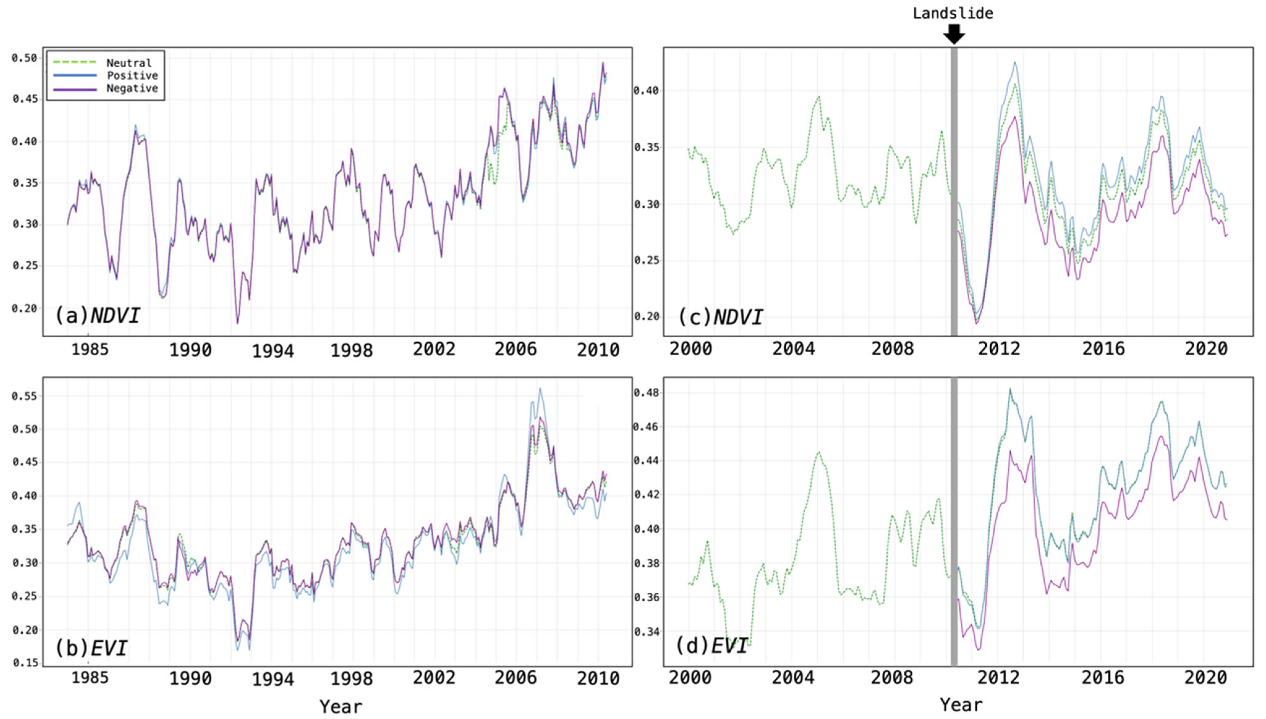
This study analyzed the effects of various environmental variables on vegetation regrowth, categorizing them as positive, neutral, and negative conditions represented by ‘+’, ‘blank’, and ‘−’, respectively, as shown in Table 7. The results are illustrated in Figure 6, where every value represents an average of the pixels in a particular group: the green dotted line represents vegetation recovery under neutral conditions, and the blue and purple lines represent vegetation recovery under positive and negative situations, respectively. The effects of different combinations of environmental variables on NDVI were not evident in Obara (Figure 6a). However, the impact of various combinations of environmental variables on EVI was more apparent than on NDVI, especially under the positive environmental condition (blue line in Figure 6b). In Shobara, the impact of different environmental factors was notable for NDVI and EVI time series trends after landslides. Specifically, the effect was more pronounced on the NDVI time series trend, whereas the unfavorable condition had a distinct impact on the EVI time series trend, different from the neutral and positive conditions (Figure 6c,d).

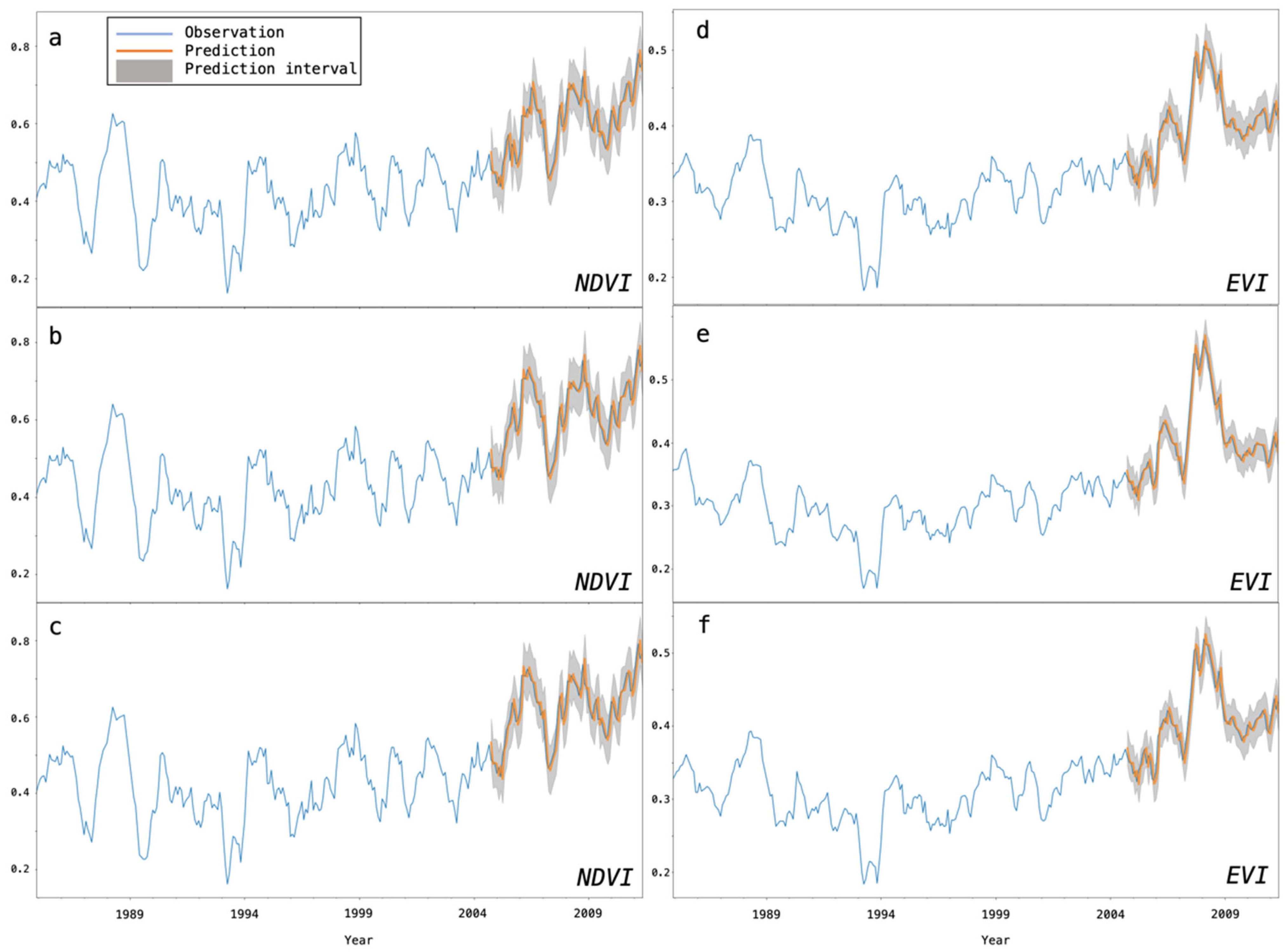
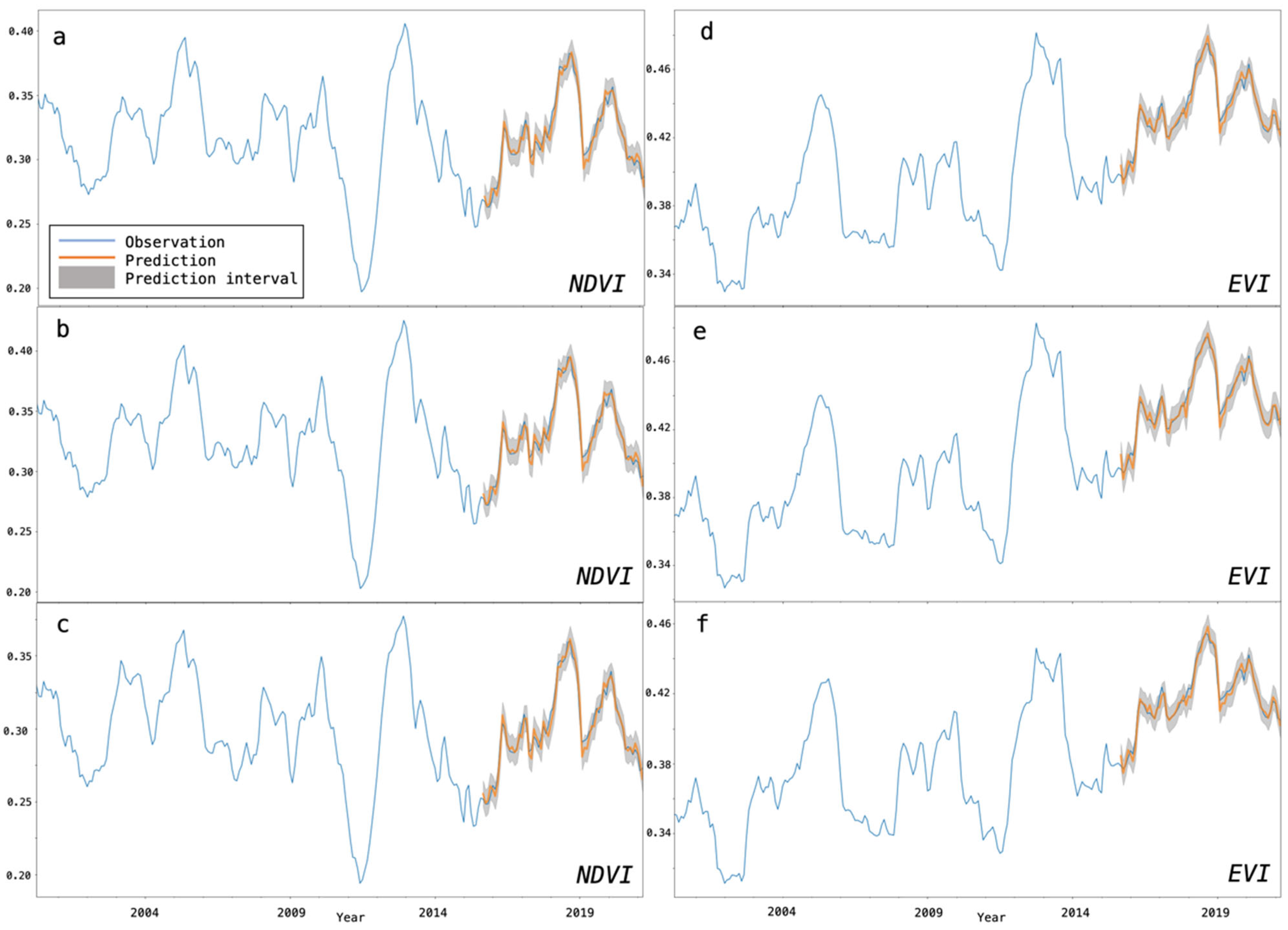
SARIMA was used to model the NDVI and EVI time series trends for the two study areas based on different combinations of environmental variables. The optimal order combination for each model was determined by feeding all the time series data into the SARIMA model and referring to the Akaike Information Criterion (AIC) value [55], commonly used to assess the relative quality of different statistical models. Three statistical indices, R², MAPE, and RMSE, were used to evaluate the performance of each model. The results are presented in

Table 8. Optimal order combination of the SARIMA model and the corresponding performance indices for each environmental condition in the Obara and Shobara districts. The subscript number in the Order line indicates a seasonal period S in Equation (5).

	NDVI			EVI
	Neutral	Positive	Negative	Neutral	Positive	Negative
Obara
Order	(1,1,0) (0,0,0)12	(1,1,0) (0,0,0)12	(1,1,0) (0,0,0)12	(1,1,0) (0,0,0)12	(1,1,0) (0,0,0)12	(1,1,0) (0,0,0)12
Train, Test	(238, 80)	(238, 80)	(238, 80)	(238, 80)	(238, 80)	(238, 80)
MAPE (%)	0.90	0.65	0.63	1.10	0.97	1.12
RMSE	0.0095	0.0070	0.0070	0.0114	0.0125	0.0118
R2	0.9738	0.9867	0.9872	0.9615	0.9650	0.9614
Shobara
Order	(1,0,1) (1,0,1)12	(2,1,1) (1,0,1)12	(2,1,1) (1,0,1)12	(1,0,1) (1,0,1)12	(2,1,1) (1,0,1)12	(1,0,1) (1,0,1)12
Train, Test	(155, 97)	(155, 97)	(155, 97)	(155, 97)	(155, 97)	(155, 97)
MAPE (%)	0.62	0.77	0.74	0.56	0.57	0.35
RMSE	0.0061	0.0080	0.0071	0.0068	0.0068	0.0041
R2	0.9739	0.9584	0.9600	0.9677	0.9678	0.9865

. Furthermore, we plotted the modeled values (orange line) of the test dataset for each model and compared them with the observed values (blue line) using 99% confidence intervals (gray area) in Figure 7 and Figure 8.

5. Discussion

5.1. Prolonged Vegetation Recovery

The NDVI and EVI trend analysis revealed that the vegetation recovery processes in the study areas exhibit a protracted duration, potentially extending beyond ten years (Figure 4 and Figure 5). This timeframe is longer than the average revegetation timescale documented in previous studies on Japan’s earthquake- and rainfall-induced landslide-affected areas [56,57,58]. Determining complete vegetation recovery in this study involves a comprehensive approach combining aerial photograph interpretation with the long-term stability of vegetation index trends. Estimating the time required for the vegetation recovery processes in Obara can be inferred by synthesizing two critical aspects of the findings. Firstly, historical aerial photograph analysis reveals that the vegetation coverage within the damaged regions remained incomplete by 1982 (Figure 5b,e). Secondly, trend analysis of NDVI and EVI calculated from Landsat imagery from 1985 to 2011 shows that both NDVI and EVI exhibited a consistent upward trend during this timeframe, influenced by seasonal fluctuations (Figure 4a,b). For Shobara, from 2011 to 2020, the observed trend revealed an upward trajectory of seasonal fluctuations in NDVI and EVI values without reaching a stable plateau of no further increase (Figure 5c,d).

The slower vegetation recovery observed in these study areas can be attributed to several factors. One is the severity of the landslide disturbance compared to the other areas. The distribution of damaged areas in both study areas is dense and extensive, and previous studies have shown a positive correlation between the disturbance magnitude and the time required for vegetation to recover fully [59,60]. The density of landslide-affected areas is around 10 and 15 patches km⁻² for Obara and Shobara, respectively, which is denser than 8–10 patches km⁻² for rainfall-induced landslides in Chiba Prefecture [56] and 5.1 patches km⁻² in the Kiso Mountains [57], central Japan. In addition, artificial vegetation was carried out on severely damaged slopes and landslide patches in the south Kiso Mountains [57]. By contrast, both study areas were left to recover naturally, extending vegetation recovery time. Therefore, the prolonged vegetation recovery can be attributed to the severity and density of the landslide disturbance and the absence of artificial vegetation interventions.

5.2. Environmental Variables Controlling Vegetation Recovery

Our analysis revealed that topographic variables (elevation, slope gradient, aspect, and curvature) significantly influenced vegetation recovery and that geological type exerted an independent influence. Previous studies have highlighted the independent impact of geological type on vegetation dynamics [61,62,63]. Different geological contexts form soil with different physical, chemical, and mineralogical properties [64,65]. Therefore, geology’s independent effect on vegetation recovery can be attributed to its influence on soil properties. However, our dataset does not enable the differentiation of soil properties, although NDVI may indicate soil reflectance to some extent [66].

For topographic variables, in Obara, rapid vegetation recovery was observed in concave and convergent terrain according to NDVI and in non-steep, low-elevation, north-facing terrain according to EVI. In Shobara, fast vegetation recovery was observed on gentler and northwest-facing slopes in terms of NDVI, and on gentler and west-facing slopes in terms of EVI. Rapid vegetation recovery in the north- to west-facing and non-steep regions may reflect higher soil moisture because of lower solar radiation (Figure 3c) [67]. Additionally, steep slope gradients may limit vegetation recovery due to limited water availability and difficulties in seed settlement and root anchoring [68]. While the elevation of the study areas did not induce significant variation in water or thermal conditions, the ANOVA results suggest that when combined with aspect or curvature, elevation may interact with vegetation recovery. Curvature shows substantial results from the three-way ANOVA (Table 6), especially in groups with slope gradients. Slightly convergent and concave terrain enhances vegetation recovery (Table 7), likely because concave depressions accumulate more water and nutrients [69,70].

Unfavorable conditions for vegetation recovery in the study areas, such as middle to upper elevations, steeper and southwest-facing slopes, and slight-divergent terrain, were widespread in the landslide-affected areas (Figure 3) and contributed to the delayed vegetation recovery observed in Section 5.1. The cumulative effect of these conditions exacerbates challenges for revegetation, including limited resources, heightened erosion risk, and reduced microclimatic suitability.

5.3. Comparisons of NDVI and EVI

This study utilized NDVI and EVI for monitoring vegetation recovery in damaged areas. NDVI is sensitive to atmospheric effects, such as cloud-induced variations [71]. Although the Landsat cloud mask helps mitigate cloud properties in per-pixel reflectance, it does not entirely eliminate bias in time series analysis [72]. On the other hand, EVI tends to show higher values in sparsely vegetated areas than NDVI [71], as NDVI is sensitive to the spectral effects of soil moisture and texture in sparsely vegetated areas [73,74]. Therefore, the high frequency of cloud cover and low vegetation coverage in Shobara has led to more pronounced differences between EVI and NDVI than in Obara (Figure 4). The greater variation in the distribution of NDVI changes (Table 3) may also reflect the high sensitivity of NDVI to soil moisture and texture [73,74].

The Shobara and Obara districts represent the early and middle-late stages of vegetation recovery, respectively. As vegetation recovery progresses, ecosystems exhibit increased resilience, diversity, and stability, leading to a decreased sensitivity to variations in environmental conditions [75] and a more consistent trend in the NDVI (Figure 6a). Although EVI was proposed to reduce atmospheric and soil background noise simultaneously, it was found to be sensitive to different environmental conditions in the two study areas (Figure 6). This may result from the soil adjustment factor in EVI that makes it more susceptible to topographic effects than NDVI [18]. Table 8 indicates that EVI outperforms NDVI in Shobara in modeling vegetation recovery trends under different environmental conditions, as the smaller MAPE value suggests. EVI incorporates the blue band, which minimizes atmospheric influences and improves sensitivity to changes in vegetation structure and density [18]. This makes EVI particularly suitable for capturing changes in early-stage vegetation conditions characterized by low structure and density, visible soil, and sparse vegetation cover. On the other hand, in Obara, NDVI demonstrates superior performance, as indicated by the lower MAPE value and higher R² value. This observation suggests that NDVI is better suited for modeling the middle and late stages of vegetation recovery within 10–25 years after the landslide. Previous studies have also reported the effectiveness of NDVI in assessing long-term vegetation dynamics in landslide-affected areas under different environmental conditions [76,77]. In addition, the Landsat time series we obtained for Obara has less cloud cover than the Shobara time series, leading to the superior performance of NDVI in Obara. However, cloud cover and its impact on NDVI do not undermine the overall effectiveness of NDVI in modeling longer-term vegetation recovery. It highlights the need to consider environmental conditions when interpreting NDVI data. Therefore, choosing appropriate and even different vegetation indices is necessary for modeling specific stages of vegetation recovery.

6. Conclusions

This study investigated vegetation recovery following rainfall-induced landslides in two areas of Japan, the Shobara and Obara districts, using Landsat data to derive NDVI and EVI time series. We found that vegetation recovery was gradual and consistent, taking over a decade without reaching a near-stable state, exceeding the previously reported vegetation recovery time for landslide-affected areas in Japan. This was caused by the severity of landslide disturbance, lack of restoration work, and the widespread occurrence of unfavorable environmental conditions. Statistical analysis of environmental variables showed that elevation, slope gradient, aspect, and curvature significantly correlated with NDVI and EVI responses in both study areas. The SARIMA model performed well in modeling NDVI and EVI under different environmental conditions. We also found that NDVI is more suitable for modeling the middle and late stages of vegetation recovery within 10–25 years after the landslide for various environmental conditions. In contrast, EVI is more suitable for modeling the early stages within 10 years after the landslides. NDVI provides insights into the long-term health and maturity of the recovering vegetation, while EVI helps capture the initial vegetation growth patterns. These results successfully addressed the primary motivation of investigating vegetation recovery and identifying suitable vegetation indices to understand post-landslide vegetation dynamics while considering the complex relationship between topography and vegetation over time. The study’s findings allow for targeted and nuanced monitoring and assessment of vegetation dynamics, enabling effective management and decision making in post-landslide ecosystems.

This study acknowledges several limitations. Firstly, Obara’s lack of certain data restricted the analysis to satellite imagery and aerial photographs, limiting the comprehensive assessment. Future studies should consider incorporating higher-resolution imagery or Light Detection and Ranging (LiDAR) data to enhance correlations with vegetation characteristics. To enhance data quality, integrating Sentinel data with Landsat imagery [78,79] can improve the accuracy of future vegetation dynamics estimates. Additionally, the contrasting results between NDVI and EVI in modeling vegetation recovery under different conditions require further investigation through additional data collection, such as soil moisture and local climate data, to better understand the underlying mechanisms. Meanwhile, further research is needed to investigate the reciprocal influences of geomorphic processes on vegetation dynamics by simulating topographic changes, enhancing the comprehension of the intricate relationship between vegetation recovery and topography. Finally, although regression models have helped to capture general trends in vegetation recovery in Obara and Shobara, future studies could consider exploring advanced approaches, such as long short-term memory (LSTM) networks, to better understand the complex nature of vegetation recovery in these regions.

References

- Saito, H.; Nakayama, D.; Matsuyama, H. Relationship between the initiation of a shallow landslide and rainfall intensity—Duration thresholds in Japan. Geomorphology 2010, 118, 167–175. [Google Scholar] [CrossRef]
- Dahal, R.K.; Hasegawa, S.; Nonomura, A.; Yamanaka, M.; Masuda, T.; Nishino, K. Failure characteristics of rainfall-induced shallow landslides in granitic terrains of Shikoku Island of Japan. Environ. Geol. 2009, 56, 1295–1310. [Google Scholar] [CrossRef]
- Van Beek, L.P.H.; Van Asch, T.W.J. Regional Assessment of the Effects of Land-Use Change on Landslide Hazard by Means of Physically Based Modelling. Nat. Hazards 2004, 31, 289–304. [Google Scholar] [CrossRef]
- Wulder, M.A.; White, J.C.; Goward, S.N.; Masek, J.G.; Irons, J.R.; Herold, M.; Cohen, W.B.; Loveland, T.R.; Woodcock, C.E. Landsat continuity: Issues and opportunities for land cover monitoring. Remote Sens. Environ. 2008, 112, 955–969. [Google Scholar] [CrossRef]
- Hermosilla, T.; Wulder, M.A.; White, J.C.; Coops, N.C.; Hobart, G.W.; Campbell, L.B. Mass data processing of time series Landsat imagery: Pixels to data products for forest monitoring. Int. J. Digit. Earth 2016, 9, 1035–1054. [Google Scholar] [CrossRef] [Green Version]
- McDowell, N.G.; Coops, N.C.; Beck, P.S.A.; Chambers, J.Q.; Gangodagamage, C.; Hicke, J.A.; Huang, C.-Y.; Kennedy, R.; Krofcheck, D.J.; Litvak, M.; et al. Global Satellite Monitoring of Climate-Induced Vegetation Disturbances. Trends Plant Sci. 2015, 20, 114–123. [Google Scholar] [CrossRef] [Green Version]
- Frost, G.V.; Epstein, H.E.; Walker, D.A. Regional and landscape-scale variability of Landsat-observed vegetation dynamics in northwest Siberian tundra. Environ. Res. Lett. 2014, 9, 025004. [Google Scholar] [CrossRef] [Green Version]
- Wang, Z.; Schaaf, C.B.; Sun, Q.; Kim, J.; Erb, A.M.; Gao, F.; Román, M.O.; Yang, Y.; Petroy, S.; Taylor, J.R.; et al. Monitoring land surface albedo and vegetation dynamics using high spatial and temporal resolution synthetic time series from Landsat and the MODIS BRDF/NBAR/albedo product. Int. J. Appl. Earth Obs. Geoinf. 2017, 59, 104–117. [Google Scholar] [CrossRef]
- Hwang, T.; Song, C.; Bolstad, P.V.; Band, L.E. Downscaling real-time vegetation dynamics by fusing multi-temporal MODIS and Landsat NDVI in topographically complex terrain. Remote Sens. Environ. 2011, 115, 2499–2512. [Google Scholar] [CrossRef]
- Jiao, Q.; Zhang, B.; Liu, L.; Li, Z.; Yue, Y.; Hu, Y. Assessment of spatio-temporal variations in vegetation recovery after the Wenchuan earthquake using Landsat data. Nat. Hazards 2014, 70, 1309–1326. [Google Scholar] [CrossRef]
- Kennedy, R.E.; Yang, Z.; Cohen, W.B. Detecting trends in forest disturbance and recovery using yearly Landsat time series: 1. LandTrendr—Temporal segmentation algorithms. Remote Sens. Environ. 2010, 114, 2897–2910. [Google Scholar] [CrossRef]
- Villarreal, M.L.; Norman, L.M.; Buckley, S.; Wallace, C.S.; Coe, M.A. Multi-index time series monitoring of drought and fire effects on desert grasslands. Remote Sens. Environ. 2016, 183, 186–197. [Google Scholar] [CrossRef] [Green Version]
- Morresi, D.; Vitali, A.; Urbinati, C.; Garbarino, M. Forest Spectral Recovery and Regeneration Dynamics in Stand-Replacing Wildfires of Central Apennines Derived from Landsat Time Series. Remote Sens. 2019, 11, 308. [Google Scholar] [CrossRef] [Green Version]
- Tucker, C.J. Red and photographic infrared linear combinations for monitoring vegetation. Remote Sens. Environ. 1979, 8, 127–150. [Google Scholar] [CrossRef]
- Huete, A.; Didan, K.; Miura, T.; Rodriguez, E.P.; Gao, X.; Ferreira, L.G. Overview of the radiometric and biophysical performance of the MODIS vegetation indices. Remote Sens. Environ. 2002, 83, 195–213. [Google Scholar] [CrossRef]
- Gao, X.; Huete, A.R.; Ni, W.; Miura, T. Optical–Biophysical Relationships of Vegetation Spectra without Background Contamination. Remote Sens. Environ. 2000, 74, 609–620. [Google Scholar] [CrossRef]
- Li, Z.; Li, X.; Wei, D.; Xu, X.; Wang, H. An assessment of correlation on MODIS-NDVI and EVI with natural vegetation coverage in Northern Hebei Province, China. Procedia Environ. Sci. 2010, 2, 964–969. [Google Scholar] [CrossRef] [Green Version]
- Matsushita, B.; Yang, W.; Chen, J.; Onda, Y.; Qiu, G. Sensitivity of the Enhanced Vegetation Index (EVI) and Normalized Difference Vegetation Index (NDVI) to Topographic Effects: A Case Study in High-density Cypress Forest. Sensors 2007, 7, 2636–2651. [Google Scholar] [CrossRef] [Green Version]
- Riva, M.J.; Daliakopoulos, I.N.; Eckert, S.; Hodel, E.; Liniger, H. Assessment of land degradation in Mediterranean forests and grazing lands using a landscape unit approach and the normalized difference vegetation index. Appl. Geogr. 2017, 86, 8–21. [Google Scholar] [CrossRef]
- Ireland, G.; Petropoulos, G.P. Exploring the relationships between post-fire vegetation regeneration dynamics, topography and burn severity: A case study from the Montane Cordillera Ecozones of Western Canada. Appl. Geogr. 2015, 56, 232–248. [Google Scholar] [CrossRef]
- Lawrence, R.L.; Ripple, W.J. Fifteen Years of Revegetation of Mount St. Helens: A Landscape-Scale Analysis. Ecology 2000, 81, 2742–2752. [Google Scholar] [CrossRef]
- Hwang, T.; Song, C.; Vose, J.M.; Band, L.E. Topography-mediated controls on local vegetation phenology estimated from MODIS vegetation index. Landsc. Ecol. 2011, 26, 541–556. [Google Scholar] [CrossRef]
- Langbein, W.B.; Schumm, S.A. Yield of sediment in relation to mean annual precipitation. Trans. Am. Geophys. Union 1958, 39, 1076–1084. [Google Scholar] [CrossRef] [Green Version]
- Srivastava, A.; Yetemen, O.; Saco, P.M.; Rodriguez, J.F.; Kumari, N.; Chun, K.P. Influence of orographic precipitation on coevolving landforms and vegetation in semi-arid ecosystems. Earth Surf. Process. Landf. 2022, 47, 2846–2862. [Google Scholar] [CrossRef]
- Saco, P.M.; Moreno-De Las Heras, M. Ecogeomorphic coevolution of semiarid hillslopes: Emergence of banded and striped vegetation patterns through interaction of biotic and abiotic processes. Water Resour. Res. 2013, 49, 115–126. [Google Scholar] [CrossRef]
- Zeng, Y.; Hao, D.; Huete, A.; Dechant, B.; Berry, J.; Chen, J.M.; Joiner, J.; Frankenberg, C.; Ben Bond-Lamberty, B.; Ryu, Y.; et al. Optical vegetation indices for monitoring terrestrial ecosystems globally. Nat. Rev. Earth Environ. 2022, 3, 477–493. [Google Scholar] [CrossRef]
- Sader, S.A.; Waide, R.B.; Lawrence, W.T.; Joyce, A.T. Tropical forest biomass and successional age class relationships to a vegetation index derived from Landsat TM data. Remote Sens. Environ. 1989, 28, 143–156. [Google Scholar] [CrossRef]
- Lai, R.; Oguchi, T.; Zhong, C. Evaluating Spatiotemporal Patterns of Post-Eruption Vegetation Recovery at Unzen Volcano, Japan, from Landsat Time Series. Remote Sens. 2022, 14, 5419. [Google Scholar] [CrossRef]
- Tobe, H.; Chigira, M. Causes of Shallow Landslides of Weathered Granitic Rocks–From the View Point of Weathering Styles and Petrologic Textures. Disaster Mitigation of Debris Flows, Slope Failures and Landslides; Universal Academy Press: Tokyo, Japan, 2006; pp. 493–501. [Google Scholar]
- Durgin, P.B. Landslides and the weathering of granitic rocks. In Landslide; The Geological Society of America: Boulder, CO, USA, 1977; Volume 3, pp. 127–131. [Google Scholar] [CrossRef]
- Onda, Y. Underlying Rock Type Controls of Hydrological Processes and Shallow Landslide Occurrence; IAHS Publication: Wallingford, UK, 1993; pp. 47–55. [Google Scholar]
- Kazukuni, K. Development of Vegetation at Some Landslides. Soc. Nat. Sci. Lib. Arts Ser. 1980, 31, 57–68. [Google Scholar]
- Okada, Y.; Kurokawa, U. Examining effects of tree roots on shearing resistance in shallow landslides triggered by heavy rainfall in Shobara in 2010. J. For. Res. 2015, 20, 230–235. [Google Scholar] [CrossRef]
- Masahiro, K.; Yoshiharu, I.; Yoshifumi, S.; Kazuki, M.; Kana, N.; Yuji, H.; Naoki, M.; Teruyoshi, T.; Kozaburo, F.; Kosuke, Y.; et al. Sediment-Related Disasters Induced by a Heavy Rainfall in Hiroshima-City on 20th August, 2014. J. Jpn. Soc. Eros. Control. Eng. 2014, 67, 49–59. [Google Scholar]
- Gorelick, N.; Hancher, M.; Dixon, M.; Ilyushchenko, S.; Thau, D.; Moore, R. Google Earth Engine: Planetary-scale geospatial analysis for everyone. Remote Sens. Environ. 2017, 202, 18–27. [Google Scholar] [CrossRef]
- Griffiths, R.P.; Madritch, M.D.; Swanson, A.K. The effects of topography on forest soil characteristics in the Oregon Cascade Mountains (USA): Implications for the effects of climate change on soil properties. For. Ecol. Manag. 2009, 257, 1–7. [Google Scholar] [CrossRef]
- Baartman, J.E.M.; Temme, A.J.A.M.; Saco, P.M. The effect of landform variation on vegetation patterning and related sediment dynamics. Earth Surf. Process. Landf. 2018, 43, 2121–2135. [Google Scholar] [CrossRef] [Green Version]
- Masek, J.G.; Vermote, E.F.; Saleous, N.E.; Wolfe, R.; Hall, F.G.; Huemmrich, K.F.; Gao, F.; Kutler, J.; Lim, T.K. A Landsat surface reflectance dataset for North America, 1990–2000. IEEE Geosci. Remote Sens. Lett. 2006, 3, 68–72. [Google Scholar] [CrossRef]
- Roy, D.P.; Kovalskyy, V.; Zhang, H.K.; Vermote, E.F.; Yan, L.; Kumar, S.S.; Egorov, A. Characterization of Landsat-7 to Landsat-8 reflective wavelength and normalized difference vegetation index continuity. Remote Sens. Environ. 2016, 185, 57–70. [Google Scholar] [CrossRef] [Green Version]
- Huete, A.R.; Didan, K.; Huete, A.; Didan, K.; Van Leeuwen, W.; Jacobson, A.; Solanos, R.; Laing, T. MODIS Vegetation Index (MOD13). Algorithm Theor. Basis Doc. 1999, 3, 295–309. [Google Scholar]
- Purevdorj, T.S.; Tateishi, R.; Ishiyama, T.; Honda, Y. Relationships between percent vegetation cover and vegetation indices. Int. J. Remote Sens. 1998, 19, 3519–3535. [Google Scholar] [CrossRef]
- Diaz-Delgado, R.; Da Cruz, R.; Salvador, L.; Pons, X. Monitoring of Plant Community Regeneration after Fire by Remote Sensing. In Fire Management and Landscape Ecology; International Association of Wildland Fire: Missoula, MT, USA, 1998; pp. 315–324. Available online: https://www.researchgate.net/profile/Ricardo-Diaz-Delgado/publication/263168534_Monitoring_of_plant_community_regeneration_after_fire_by_remote_sensing/links/00b4953a16fb02f2e0000000/Monitoring-of-plant-community-regeneration-after-fire-by-remote-sensing.pdf (accessed on 27 July 2023).
- Veraverbeke, S.; Gitas, I.; Katagis, T.; Polychronaki, A.; Somers, B.; Goossens, R. Assessing post-fire vegetation recovery using red–near infrared vegetation indices: Accounting for background and vegetation variability. ISPRS J. Photogramm. Remote Sens. 2012, 68, 28–39. [Google Scholar] [CrossRef] [Green Version]
- Huete, A.R. A soil-adjusted vegetation index (SAVI). Remote Sens. Environ. 1988, 25, 295–309. [Google Scholar] [CrossRef]
- Martín-Ortega, P.; García-Montero, L.G.; Sibelet, N. Temporal Patterns in Illumination Conditions and Its Effect on Vegetation Indices Using Landsat on Google Earth Engine. Remote Sens. 2020, 12, 211. [Google Scholar] [CrossRef] [Green Version]
- Gao, M.-L.; Zhao, W.-J.; Gong, Z.-N.; Gong, H.-L.; Chen, Z.; Tang, X.-M. Topographic Correction of ZY-3 Satellite Images and Its Effects on Estimation of Shrub Leaf Biomass in Mountainous Areas. Remote Sens. 2014, 6, 2745–2764. [Google Scholar] [CrossRef] [Green Version]
- Van Leeuwen, W.J.D. Monitoring the Effects of Forest Restoration Treatments on Post-Fire Vegetation Recovery with MODIS Multitemporal Data. Sensors 2008, 8, 2017–2042. [Google Scholar] [CrossRef] [PubMed] [Green Version]
- Riaño, D.; Chuvieco, E.; Ustin, S.; Zomer, R.; Dennison, P.; Roberts, D.; Salas, J. Assessment of vegetation regeneration after fire through multitemporal analysis of AVIRIS images in the Santa Monica Mountains. Remote Sens. Environ. 2002, 79, 60–71. [Google Scholar] [CrossRef]
- Huete, A.R.; Liu, H.Q.; Batchily, K.; Van Leeuwen, W. A comparison of vegetation indices over a global set of TM images for EOS-MODIS. Remote Sens. Environ. 1997, 59, 440–451. [Google Scholar] [CrossRef]
- U.S. Geological Survey Landsat Enhanced Vegetation Index. Available online: https://www.usgs.gov/landsat-missions/landsat-enhanced-vegetation-index (accessed on 1 April 2021).
- Abdi, H.; Williams, L.J. Tukey’s Honestly Significant Difference (HSD) Test. Encycl. Res. Des. 2010, 3, 1–5. [Google Scholar]
- Kendall, M.G. A New Measure of Rank Correlation. Biometrika 1938, 30, 81–93. [Google Scholar] [CrossRef]
- Box, G. Box and Jenkins: Time Series Analysis, Forecasting and Control. In A Very British Affair: Six Britons and the Development of Time Series Analysis during the 20th Century; Springer: London, UK, 2013; pp. 161–215. [Google Scholar]
- Alhamad, M.N.; Stuth, J.; Vannucci, M. Biophysical modelling and NDVI time series to project near-term forage supply: Spectral analysis aided by wavelet denoising and ARIMA modelling. Int. J. Remote Sens. 2007, 28, 2513–2548. [Google Scholar] [CrossRef]
- Bozdogan, H. Model selection and Akaike’s Information Criterion (AIC): The general theory and its analytical extensions. Psychometrika 1987, 52, 345–370. [Google Scholar] [CrossRef]
- Shinya, N.; Masakazu, S.; Miki, N.; Koichiro, K.; Tsuguo, S.; Takehiko, O. Monitoring of Revegetation after Slope Failure Using Aerial photography–A 25-Year Trend in Slope Failure Sites Created by the Southern Bousou Storm in 1970. Jpn. Soc. Eros. Control. Eng. 1999, 52, 14–20. [Google Scholar]
- Yoshinori, T.; Izumi, K.; Hideki, T.; Itsurou, I.; Masumi, O.; Takashi, F. Process of Occurrence and Recovery of Surface Soil Slides–An Analysis in “Preliminary Area of Erosion Front” of Mountain Devastation Model. Jpn. Soc. Eros. Control. Eng. 2001, 54, 63–72. [Google Scholar]
- Saito, H.; Uchiyama, S.; Teshirogi, K. Rapid vegetation recovery at landslide scars detected by multitemporal high-resolution satellite imagery at Aso volcano, Japan. Geomorphology 2022, 398, 107989. [Google Scholar] [CrossRef]
- Johansen, M.P.; Hakonson, T.E.; Breshears, D.D. Post-fire runoff and erosion from rainfall simulation: Contrasting forests with shrublands and grasslands. Hydrol. Process. 2001, 15, 2953–2965. [Google Scholar] [CrossRef]
- Montgomery, D.R.; Dietrich, W.E. A physically based model for the topographic control on shallow landsliding. Water Resour. Res. 1994, 30, 1153–1171. [Google Scholar] [CrossRef]
- Marston, R.A. Geomorphology and vegetation on hillslopes: Interactions, dependencies, and feedback loops. Geomorphology 2010, 116, 206–217. [Google Scholar] [CrossRef]
- Major, J. A Functional, Factorial Approach to Plant Ecology. Ecology 1951, 32, 392–412. [Google Scholar] [CrossRef]
- Kulkarni, A.; Shetti, R.; Shigwan, B.K.; Vijayan, S.; Datar, M.N. What determines vegetation on rock outcrops of the Western Ghats: The macro-environment or lithotype? Folia Geobot. 2021, 56, 149–165. [Google Scholar] [CrossRef]
- Da Silva, Y.J.A.B.; Do Nascimento, C.W.A.; Biondi, C.M.; van Straaten, P.; da Silva, Y.J.A.B.; de Souza, V.S.; de Araújo, J.D.C.T.; Alcantara, V.C.; da Silva, F.L.; da Silva, R.J.A.B. Concentrations of major and trace elements in soil profiles developed over granites across a climosequence in northeastern Brazil. Catena 2020, 193, 104641. [Google Scholar] [CrossRef]
- Wilson, M.J. The importance of parent material in soil classification: A review in a historical context. Catena 2019, 182, 104131. [Google Scholar] [CrossRef]
- Huete, A.R.; Jackson, R.D.; Post, D.F. Spectral response of a plant canopy with different soil backgrounds. Remote Sens. Environ. 1985, 17, 37–53. [Google Scholar] [CrossRef]
- Nadal-Romero, E.; Petrlic, K.; Verachtert, E.; Bochet, E.; Poesen, J. Effects of slope angle and aspect on plant cover and species richness in a humid Mediterranean badland. Earth Surf. Process. Landf. 2014, 39, 1705–1716. [Google Scholar] [CrossRef]
- Lin, C.-Y.; Lo, H.-M.; Chou, W.-C.; Lin, W.-T. Vegetation recovery assessment at the Jou-Jou Mountain landslide area caused by the 921 Earthquake in Central Taiwan. Ecol. Model. 2004, 176, 75–81. [Google Scholar] [CrossRef]
- Florinsky, I.V.; Kuryakova, G.A. Influence of topography on some vegetation cover properties. Catena 1996, 27, 123–141. [Google Scholar] [CrossRef]
- Mörsdorf, M.A.; Ravolainen, V.T.; Yoccoz, N.G.; Thórhallsdóttir, T.E.; Jónsdóttir, I.S. Decades of Recovery from Sheep Grazing Reveal No Effects on Plant Diversity Patterns within Icelandic Tundra Landscapes. Front. Ecol. Evol. 2021, 8, 602538. [Google Scholar] [CrossRef]
- Song, C.; Woodcock, C.E. Monitoring forest succession with multitemporal Landsat images: Factors of uncertainty. IEEE Trans. Geosci. Remote Sens. 2003, 41, 2557–2567. [Google Scholar] [CrossRef]
- Holden, C.E.; Woodcock, C.E. An analysis of Landsat 7 and Landsat 8 underflight data and the implications for time series investigations. Remote Sens. Environ. 2016, 185, 16–36. [Google Scholar] [CrossRef] [Green Version]
- Kremer, R.G.; Running, S.W. Community type differentiation using NOAA/AVHRR data within a sagebrush-steppe ecosystem. Remote Sens. Environ. 1993, 46, 311–318. [Google Scholar] [CrossRef]
- Schmidt, H.; Karnieli, A. Remote sensing of the seasonal variability of vegetation in a semi-arid environment. J. Arid. Environ. 2000, 45, 43–59. [Google Scholar] [CrossRef] [Green Version]
- Oliver, T.H.; Heard, M.S.; Isaac, N.J.B.; Roy, D.B.; Procter, D.; Eigenbrod, F.; Freckleton, R.P.; Hector, A.L.; Orme, C.D.L.; Petchey, O.; et al. Biodiversity and Resilience of Ecosystem Functions. Trends Ecol. Evol. 2015, 30, 673–684. [Google Scholar] [CrossRef] [Green Version]
- Chen, M.; Tang, C.; Li, M.; Xiong, J.; Luo, Y.; Shi, Q.; Zhang, X.; Tie, Y.; Feng, Q. Changes of surface recovery at coseismic landslides and their driving factors in the Wenchuan earthquake-affected area. Catena 2022, 210, 105871. [Google Scholar] [CrossRef]
- Chen, T.-H.K.; Prishchepov, A.V.; Fensholt, R.; Sabel, C.E. Detecting and monitoring long-term landslides in urbanized areas with nighttime light data and multi-seasonal Landsat imagery across Taiwan from 1998 to 2017. Remote Sens. Environ. 2019, 225, 317–327. [Google Scholar] [CrossRef]
- Claverie, M.; Ju, J.; Masek, J.G.; Dungan, J.L.; Vermote, E.F.; Roger, J.-C.; Skakun, S.V.; Justice, C. The Harmonized Landsat and Sentinel-2 surface reflectance data set. Remote Sens. Environ. 2018, 219, 145–161. [Google Scholar] [CrossRef]
- Chaves, M.E.D.; Picoli, M.C.A.; Sanches, I.D. Recent Applications of Landsat 8/OLI and Sentinel-2/MSI for Land Use and Land Cover Mapping: A Systematic Review. Remote Sens. 2020, 12, 3062. [Google Scholar] [CrossRef]
Figure 1.
Study areas. (a) Location of the Obara district in Japan and Toyota City, black and red boxes, respectively. (b) Shallow landslides in the Obara district from the Google World Map. (c) Location of the Shobara district in Japan and Shobara City, black and red boxes, respectively. (d) Shallow landslides in the Shobara district from the Google World Map.
Figure 2.
Extracted damaged areas distribution maps of the Obara (a) and Shobara (b) districts. The base map was referenced from the Google World Map.
Figure 3.
Frequency distribution of (a) elevation, (b) slope gradient, (c) aspect, (d) horizontal curvature, (e) maximal curvature, and (f) vertical curvature in damaged areas as calculated from the SRTM 30 m DEM.
Figure 4.
NDVI (in yellow) and EVI (in green) temporal fluctuations for landslide-affected regions. (a) Yearly average values of NDVI and EVI in Obara from 1985 to 2011; (b) monthly average values of NDVI and EVI in Obara from December 1984 to May 2012; (c) yearly average values of NDVI and EVI in Shobara from 2000 to 2020, and (d) monthly average values of NDVI and EVI in Shobara from October 1999 to September 2021. The gray line in (c,d) represents the landslide event triggered by heavy rainfall in July 2010 in Shobara.
Figure 5.
Photographs showing vegetation recovery at the same damaged region (black box in (a)) in the Obara district after the 1972 landslide; (b) 1972, (c) 1974, (d) 1977, (e) 1982, (f) 1988.
Figure 6.
Impact of environmental factors on NDVI and EVI time series trends in the Obara and Shobara districts. (a,b) show the NDVI and EVI responses in Obara, respectively; (c,d) show the NDVI and EVI responses in Shobara, respectively. The green dotted line indicates neutral conditions. The blue and purple solid lines indicate positive and negative conditions, respectively. The gray line in panels (c,d) represents the occurrence of landslides triggered by heavy rainfall in July 2010 in Shobara.
Figure 7.
Comparison between the modeled and observed values of the test datasets for each model in Obara under different environmental factor conditions: (a) NDVI with neutral conditions, (b) NDVI with positive conditions, (c) NDVI with negative conditions, (d) EVI with neutral conditions, (e) EVI with positive conditions, and (f) EVI with negative conditions. The orange line represents the modeled values, while the blue line represents the observed values. The 99% confidence intervals of the modeled values are depicted as the gray area.
Figure 8.
Comparison between the modeled and observed values of the test datasets for each model in Shobara under different environmental factor conditions: (a) NDVI with neutral conditions, (b) NDVI with positive conditions, (c) NDVI with negative conditions, (d) EVI with neutral conditions, (e) EVI with positive conditions, and (f) EVI with negative conditions. The orange line represents the modeled values, while the blue line represents the observed values. The 99% confidence intervals of the modeled values are depicted as the gray area.