
The Impact of Urban Warming on the Mortality of Vulnerable Populations in Seoul


1
Department of Architectural Engineering, Kyung Hee University, 1732 Deogyeongdaero, Yongin-si 17104, Korea
2
Faculty of Built Environment, University of New South Wales, Sydney 2052, Australia
*
Author to whom correspondence should be addressed.
Sustainability 2022, 14(20), 13452; https://doi.org/10.3390/su142013452
Submission received: 24 September 2022
/
Revised: 9 October 2022
/
Accepted: 13 October 2022
/
Published: 18 October 2022
(This article belongs to the Special Issue Urban Climate and Health)
Abstract
:Climate change influences urban mortality. The magnitude of such influences differs from locality to locality and is fundamentally driven by a facet of factors that include changes in local climatic conditions, demographics, and social-economic factors. Here, we employ regression and clustering methods to study linkages between mortality and local climatic changes in Seoul. Personal factors of the deceased (e.g., age and gender), social-economic factors (i.e., education level), and outdoor climatic factors, including heatwaves (HWs) and the urban heat island (UHI) phenomenon are considered in the analysis. We find that, among many elements of outdoor weather factors considered, the apparent temperature mostly correlated to daily mortalities; the mortality risk to apparent temperature exposure is more heightened for males (RR = 0.40, 95% CI; 0.23–0.54) than females (RR = 0.05, 95% CI; −0.10–0.20) at higher apparent temperatures (i.e., 60 °C). Furthermore, the influence of HWs on mortality is more apparent in the “Male” gender group and the “Above 65” age group. The results are useful in identifying vulnerable demographics amid the changing climate, especially in urban areas, and are fundamental in developing policies that promote climate resilience and adaptation.
1. Introduction
One significant effect of climate change is its adverse impact on human health and performance [1]. Various scientific reports provide substantial evidence relating climate change-driven temperature variations to heat and cold-related mortalities and morbidities [2,3,4]. Some recent efforts to quantify the effect of extreme temperature variations have reported increases in global temperature-related death ranging between 3% and 12.7% under future projections of greenhouse gas emissions [5]. Such effects of temperature on human health are often double-sided—extremely low temperatures promote hypothermic reactions. In contrast, extremely high temperatures induce hyperthermic reactions, which are detrimental to well-being, although the projections are seemingly more severe for warmer and poorer localities. Consequently, determining temperature balances that promote bodily homeostasis is crucial to achieving sustainable livelihoods, especially amid the changing climate.
The occurrence of heatwaves (HWs), defined as episodes of prolonged high temperatures and which are partly driven by the changing climate, also contribute significantly to heat-related mortalities and morbidities [6]. Empirical evidence demonstrating correlations between HWs, and heat-related mortality has been reported in many parts of Europe [7,8], the United States [9], Russia [10], and Korea [11]. The impact of HWs on heat-related mortalities is even more worrisome, given a vast number of scientific studies that forecast an increase in the frequency, duration, and severity of HWs in the near future.
Vulnerability to temperature-related mortalities and morbidities is more heightened in urban areas than rural areas. However, this tends to arise from extreme heat conditions than cold heat conditions and is mainly attributed to urban heat islands (UHI). UHIs refer to the often higher surface and atmospheric temperatures in urban environments than their rural, more natural surroundings [12]. UHIs arise from complex interactions between the urban form, which is primarily modified by urbanization, and urban climates that are substantially influenced by intense anthropogenic activities—such complex interactions significantly modify the urban thermal structure, intensifying extreme heat-related incidences in urban areas [13,14]. Various scientific studies have demonstrated the effects of UHI on heat-related mortality in many agglomerations. For instance, the extent of UHI impacts on heat-related mortality was reported at 1.1 deaths per million people in American cities [15]. The effect of UHI on heat-related mortalities has also been demonstrated in Athens [16], London [17], and Shanghai [18]. A more recent study conducted in multiple cities in China has shown that compound heat events are more pronounced in urban areas than their rural counterparts and such observations are potentially fueled by UHI formation [19]. Such influences of UHI on the well-being of urban populations are forecasted to worsen, considering the increasing rate of urbanization resulting in higher UHI intensities (UHII).
UHI and HWs have also been reported to interact synergistically, substantially amplifying heat-related mortalities. For instance, Founda and Santamouris reported higher UHII, reaching up to 3.5 °C, during HW periods than during normal summer conditions in Athens [20]. Such heightened UHII during HWs have also been reported in Sydney [21], Seoul [22] and multiple cities in China [23]. While the magnitude of the interdependencies between UHI and HWs is likely to differ from locality to locality given the peculiarity of each location (e.g., space form and configuration, land characteristics, etc.), the consensus in the literature points to the synergistic interactions between the two phenomena and their heightened influence on mortalities and morbidities in urban areas. This is worrisome amid increasing evidence projecting increased UHII and more frequent HWs in the near future [24].
The effects of climate change, HWs, and UHI on heat-related deaths discussed above are not equally distributed across all populations. Some populations are more affected than others, and this primarily arises from the differences in personal factors, social-economic factors, or a complex combination of the two elements. Epidemiological studies have shown that the physiological and psychological toll of extreme temperatures is higher in specific subgroups than the others [25]. For instance, the effects of high temperatures differ among age groups; temperature-related mortalities and morbidities are amplified at the extreme ends of the age curve [26]. Gender (used here and throughout the manuscript to refer to the biological differences between individuals of different sexes) has also been reported to modulate the effects of temperature on health and performance—the different responses to temperature changes between genders and age groups have been attributed to the inherent differences in physiology between genders or age groups [27,28].
Variations in how certain groups respond to temperature changes have also been attributed to occupational differences. Outdoor workers and occupations involving intense physical activities (e.g., athletes, soldiers) are more prone to temperature-related heat strokes primarily due to large amounts of metabolic heat production and heat gain intrinsic to the nature of certain occupations [29]. Energy poverty is also an issue that is increasingly having a substantial influence on the resilience of certain groups during extreme temperatures [30]. Vulnerability to heat-related health issues is highest for populations with less/insufficient access to energy resources or relevant equipment (e.g., heating ventilation and air conditioning systems).
Assessing the effect of local climatic changes on human health and performance is a challenging issue, particularly given the vast range of factors likely to modulate the said effect (i.e., UHI, HWs, personal factors, and social-economic factors) but one of urgency especially considering the changing climate. While the fundamental effects of temperature changes on heat-related mortality are properly understood in the literature, quantification of such effects is likely to vary from locality to locality, mainly due to acclimatization. Heat-related mortalities have been reported to increase substantially when temperatures deviate from the local mean [31]. Local mean temperatures vary considerably even across conurbations of similar sizes. To that end, the present study aims to explore variations in heat-related daily mortality counts in Seoul city, a densely populated and highly urbanized conurbation, considering local climatic conditions and personal and social-economic factors. The results shed more light on heat exposure-related vulnerability in Seoul city and form a basis for effective policies to combat heath issues stemming from changes in local climatic conditions.
2. Methods
2.1. Study Area
Seoul, South Korea’s capital and the most populous city in South Korea (i.e., it harbors about 21% of the country’s population) [32], was selected as the target area for the current study. It is located at a longitude of 126.59° E and latitude of 37.34° N, which is the central-western part of the Korean peninsula. Seoul’s climate falls under a combination of the humid continental and subtropical climates with relatively mid-range annual mean temperatures (i.e., 24 °C) [33]. Seoul’s urbanization rate has risen substantially, intensifying increases in local climatic changes associated with UHI. For instance, an increase of 0.7 °C over the last 30 years as reported by the Korean Meteorological Agency (KMA). Such changes in Seoul’s local climatic conditions are forecasted to worsen, given the increasing rate of urbanization and the need for extensive and dense infrastructure to cater for the said urbanization. In previous years, Seoul has also experienced several HWs and hot spells [34,35]. Such HWs, whose occurrence is projected to increase in frequency, duration, and severity, is likely to exacerbate heat-related mortalities and morbidities in Seoul. Consequently, Seoul makes for an ideal environment to assess the impact of local climatic changes on the well-being of urban dwellers in South Korea.
2.2. Mortality and Weather Data
We considered non-accidental deaths likely to be fueled by changes in climatic conditions (i.e., cardiovascular, and respiratory related deaths). Daily mortality counts due to cardiovascular and respiratory diseases were obtained from an open-source database provided by statistics Korea via a microdata service platform [36]. The platform avails the number of daily mortalities and personal details related to the deceased. Information such as age, gender, and level of education was extracted from the database and incorporated into the analysis to assess variations in temperature vulnerabilities stemming from personal differences. The data were collected for 19 years (i.e., from 1999 to 2018) to capture temporal changes in temperature-related vulnerabilities. The extended assessment period also captures the changes in urbanization, which are fundamentally linked to factors that drive changes in local climatic conditions (i.e., UHI and HW).
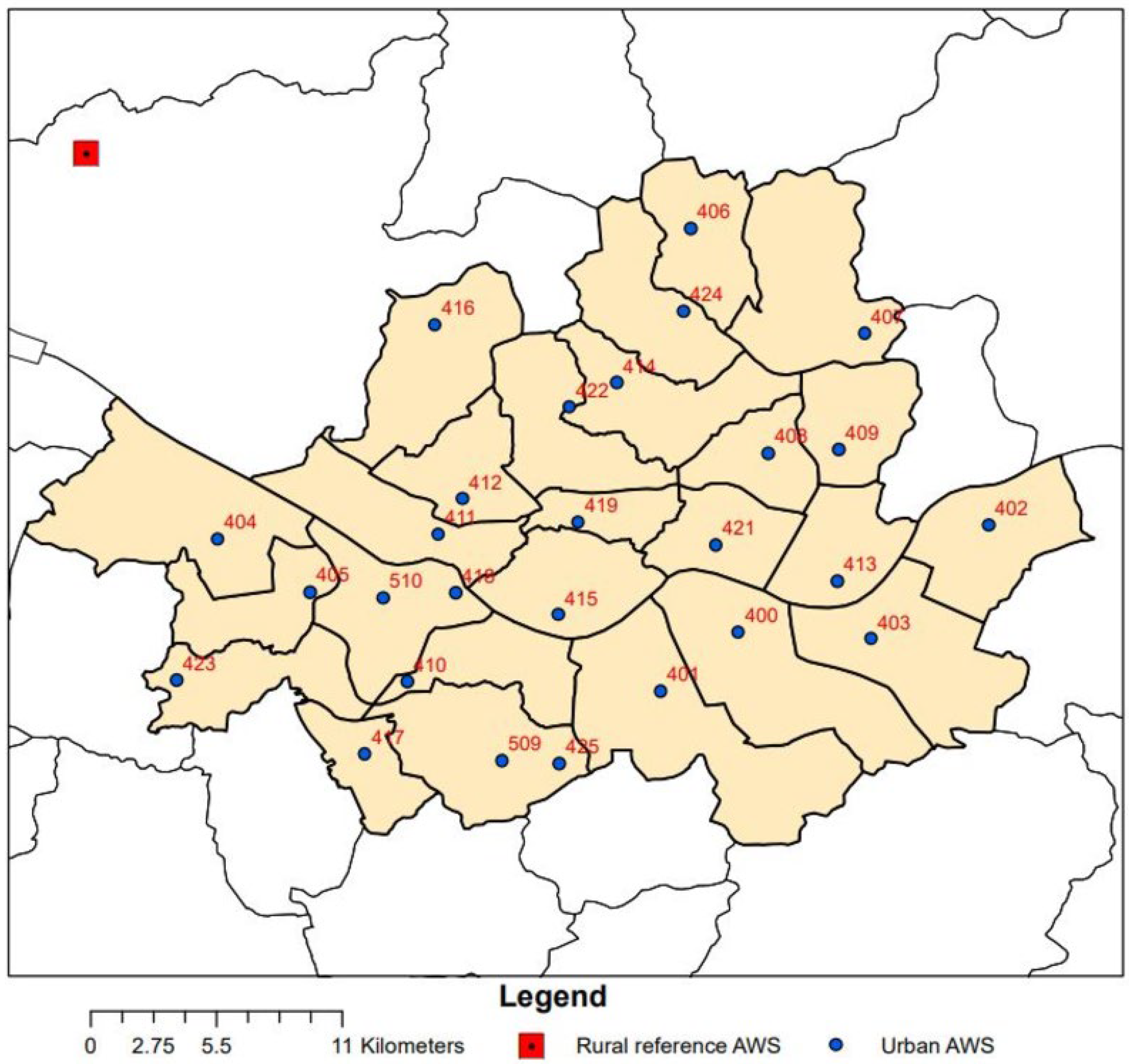
Hourly air temperature elements were also obtained from an open-source database run by the KMA [37]; these are recorded at 27 automatic weather stations (AWS) in Seoul (See Figure 1). The observatories were equipped with thin film sensors that record air temperature values in the range of −40 °C and 60 °C with an uncertainty error of 0.3 °C. To match the mortality data, hourly temperature values for 19 years were extracted.
2.3. Apparent, Mean Running and Dewpoint Temperature
As well as the temperature variants collected directly from the government platform discussed above, we also computed apparent air temperature and mean running temperature—The two variants of temperature, particularly apparent temperature, have been used consistently to quantify the impact of heat stress on mortality and health in various previous studies [38,39,40,41]. Apparent temperature considers the heat stress caused by the combined effect of temperature and humidity on the human body, while mean running temperature is a cumulative heat index that considers historical temperature values. The apparent temperature was computed from Equation (1) and mean running temperature was computed from Equation (2). Maximum dewpoint temperature is derived from ambient maximum temperature and relative humidity using a formula proposed in [42].
where = Apparent temperature, T = Outdoor air temperature, and = dewpoint temperature
where = Mean running temperature, is the mean outdoor temperature at n times—intervals previously, and α is a time constant that reflects the rate at which the effect of any past temperature decays.
2.4. Urban Heat Island (UHI) and Heatwaves (HWs)
UHI was quantified using the UHI intensity index (UHII), computed as the difference in air temperature in an urban area (Turban) and air temperature at a rural reference station (Trural). For urban temperature data, we considered hourly average values from 27 automatic weather stations run by the KMA and located in Seoul (See Figure 1); the obtained values were then averaged to obtain hourly temperature values representative of the entire Seoul. For the rural reference station, a single station, Neunggok, located on the outer boundary of Seoul at a longitude of 126.47° E and latitude of 37.37° N, was selected. The choice of the reference station was based on the World Meteorological Organization (WMO) guideline dictating that representative rural reference stations be located in relatively flat terrain with a paucity of urbanized infrastructure [43]. The chosen reference station has been used for the same role in multiple UHI studies in Seoul [44,45]. As well as being in a rural background in line with the WMO descriptions for an adequate rural reference station, it is also positioned in a manner exposing it to the same predominant wind conditions as Seoul, which further reduces potential errors in the estimation of UHI. The average distance between the considered urban AWSs and the rural reference station is 25 km. UHII was then computed as the difference in hourly temperature values between Seoul and Neuggok (see Equation (3)).
where = Urban heat island intensity, = Air temperature at an urban weather observatory, and = Air temperature at a selected reference rural weather observatory.
Furthermore, HWs are defined following the threshold by the KMA. The KMA defines a HW day as a day whose maximum temperature exceeds 33 °C. The threshold reflects the 96th percentile of the averaged daily maximum temperatures of all stations in Korea and has been the basis of multiple relevant studies in Korea [11,22,46]. In the present, a HW episode is thus defined as a period of 3 or more consecutive days whose daily maximum temperatures exceeded 33 °C (see Equation (4)).
2.5. Statistical Analysis
Several statistical analyses were conducted to determine the influence of the earlier mentioned (i) personal factors and weather elements on daily mortality counts. For instance, we conducted a regression analysis of multiple orders to analyze the variance in daily mortality counts considering multiple weather variables. Several criteria should be met to conduct a robust regression analysis (i.e., independence of observations and absence of homoscedasticity). In the present study, the independence of observations was assessed using the Durbin–Watson test [47]. Homoscedasticity was evaluated by the inspection of studentized and standardized residual plots.
Analysis of variance (ANOVA) was also employed to evaluate mean differences in daily mortality counts across different population groups (i.e., genders, age groups, and education level) and the interactive effect of several factors on daily mortality counts. ANOVA also requires that certain assumptions be met (i.e., normality of the data, homogeneity of variances, and absence of significant outliers). The present study assessed the normality assumption using the Shapiro–Wilk’s test [48], and the homogeneity test was assessed using Levine’s test [49]. When the data failed to meet the above assumptions, non-parametric approaches were used (e.g., Welch’s test of unequal variances). Moreover, to further assess the relationship between UHI and daily mortality counts, the UHI data were categorized into hierarchical clusters of increasing intensities; (i) Low UHI cluster (UHII ≤ 1 °C) (ii) Medium UHI cluster (1 °C ≤ UHII ≤ 2 °C) and (iii) High UHI cluster (UHII > 2 °C). Furthermore, to assess the relative contributions/importance of various factors on daily mortalities, we conducted a stepwise regression analysis correlating (i) time factors, (ii) weather factors, and (iii) personal factors. First, multicollinearity diagnostic analysis was conducted to identify dependencies among the different factors considered in the study—we used Pearson correlation analysis (r) to identify highly correlated variables (r > 0.8). Collinearity diagnostics were used to evaluate inter-correlations among the considered weather and personal elements using the tolerance and value inflation factor (VIF) index [50].
Additionally, we employed a generalized additive model (GAM) to estimate the rate ratio of the effect of temperature variants on the heat-related mortality of different subgroups (i.e., characterized by gender and age). GAMs are considered extensive versions of generalized linear models with high flexibility and potential to adjust for non-linearities often associated with time-series data (e.g., seasonality)—they are mathematically represented by the equations below and have been widely employed in modeling the effect of environmental conditions on mortality [41,51].
where represents the daily number of heat-related mortalities, is the coefficients of temperature variants. At the same time, denotes the relative log rate of death counts per unit change in temperature variation. represents the smoothing functions of other cofounding parameters (e.g., UHI, HWs). The modeling was conducted using the mgcv package in R. Relative risk is inherently determined as exp () at a 95% confidence interval (CI) and refers to the probability risk of mortality associated with a certain regressor. The analysis presented in the current study was conducted using R studio, version R-4.0.2.
3. Results
3.1. Variations in Daily Mortality Counts Grouped by Gender and Season
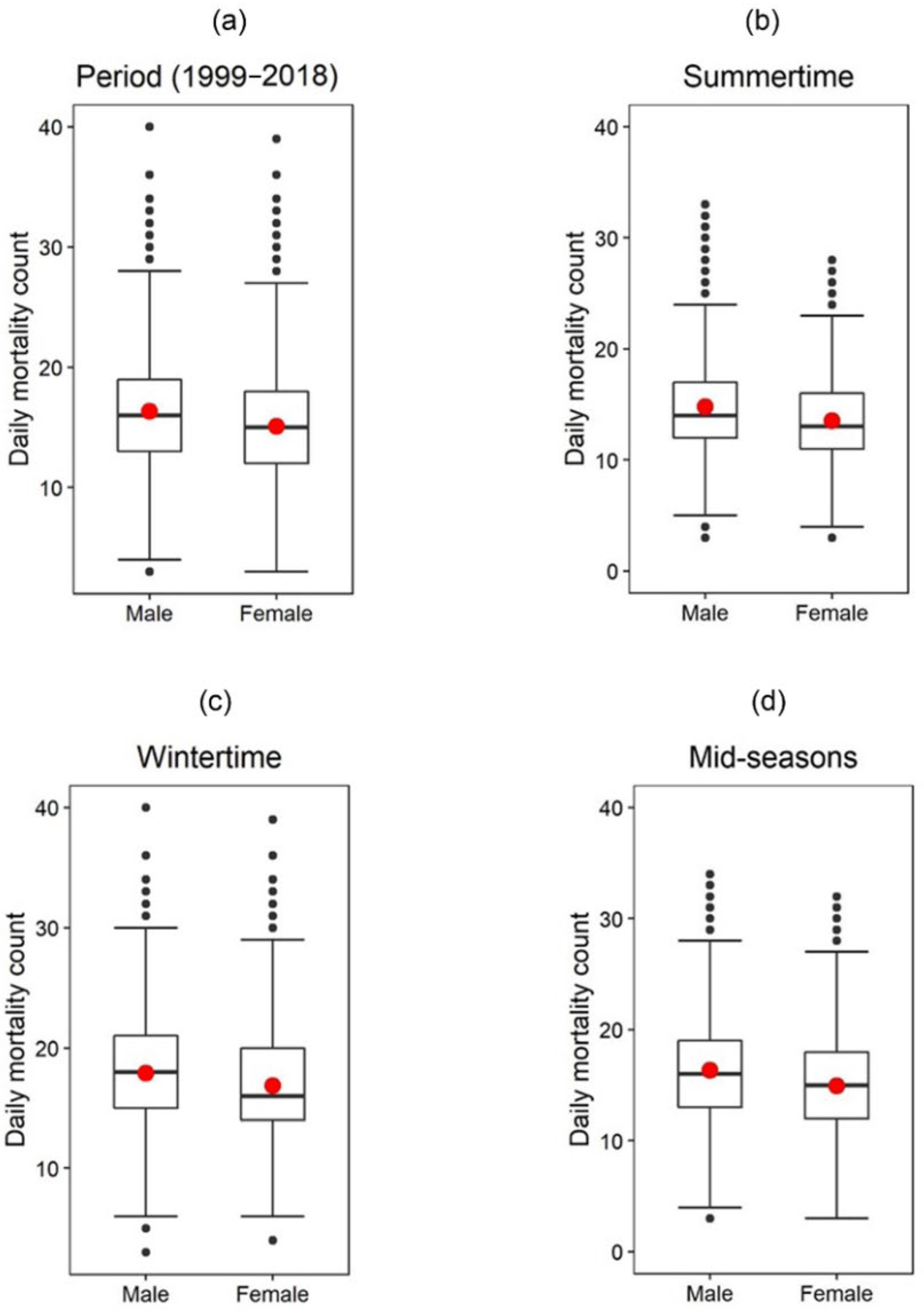
Figure 2 shows daily cardiovascular and respiratory disease variations grouped by gender and season; the specific values are reported as mean (M) ± standard deviation (SD). Considering the entire period (i.e.,1999–2018), daily mortalities were slightly higher for males (16.35 ± 4.55) than females (15.07 ± 4.39); these differences were also statistically significant F(1,14608) = 299.28, p < 0.05. The slightly higher mortality counts in males than females are consistent throughout all the seasons (i.e., summertime, wintertime, and mid-seasons) and, via a one-way ANOVA analysis, the observed differences are statistically significant across the seasons (See Table 1). Moreover, from the figure, it is observed that the highest number of daily mortalities, regardless of gender, occurred in the wintertime.
3.2. Variations in Daily Mortality Counts Grouped by Age, Gender, and Season
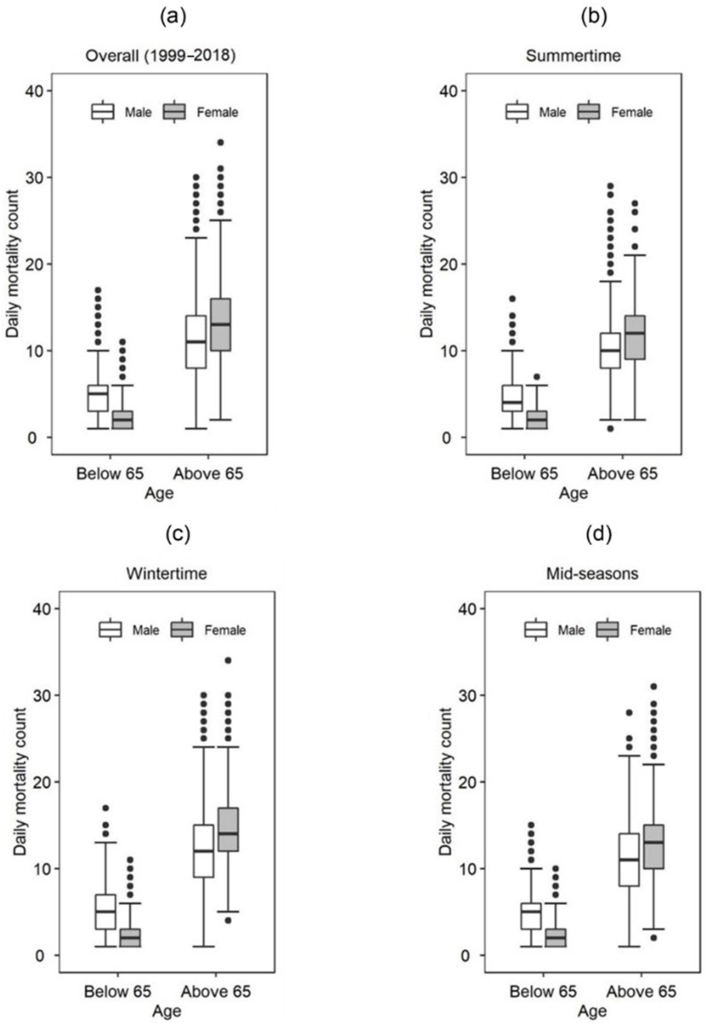
Figure 3 shows variations in seasonal daily mortality counts considering age and gender. The analysis focuses on a cutoff age boundary of 65 years because multiple previous studies have reported the age group above 65 years of age as the demographic mostly susceptible to temperature-related mortalities [16,52,53,54,55]. From the figure, it is observed that daily mortality counts are higher in the “Above 65” age group than the “Below 65” age group and seem to be modulated by gender and season. For example, the highest median mortality counts were observed for females above 65 years of age during the winter season (14 ± 4.40) while the lowest median mortality counts belonged to the group of females “Below 65” and seemed consistent throughout the seasons (i.e., approximately 2 ± 1.4). This indicates that the most vulnerable group are females above 65 years of age. Interestingly, in the “Above 65” age group, daily mortality counts were higher for females than males, whereas the opposite was true in the “Below 65” age group. A two-way ANOVA indicated that age was much more related to daily cardiovascular and respiratory mortality counts, particularly in the wintertime (F(1,3) = 13,056.27, p-value < 0.05, Partial η² = 0.65) than the other seasons. Furthermore, the results showed age to have a higher impact on daily mortalities than gender, while the interactive effect of the two factors showed small but statistically significant influences (See Table 2).
3.3. Effect of Outdoor Weather Conditions on Daily Mortality Counts
3.3.1. Minimum Temperature
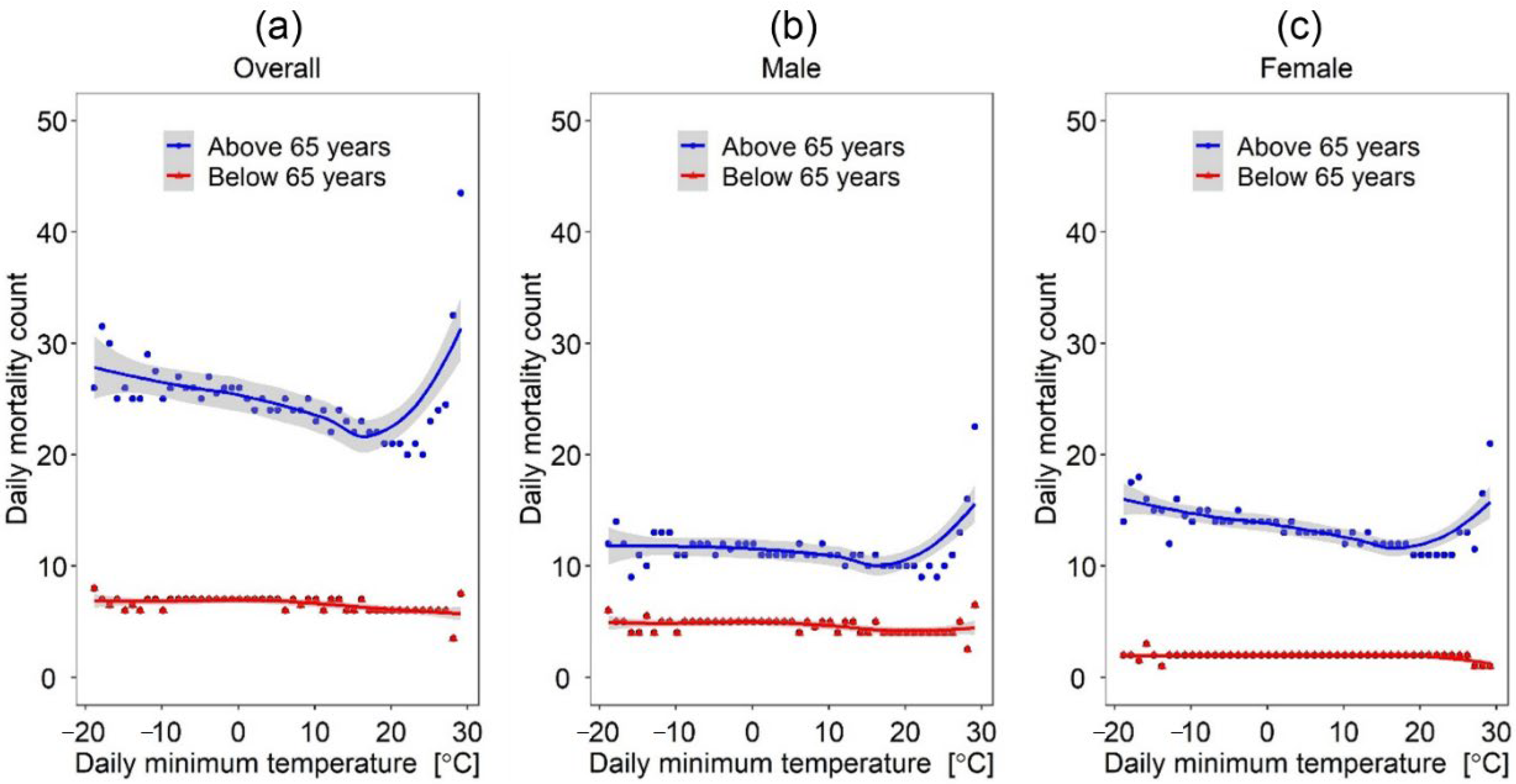
Figure 4 shows the changes in daily mortality counts as a function of daily minimum temperature grouped by age and gender. As observed from the figures, the relationship between daily mortality counts and daily minimum temperature is somewhat modified by age and gender. Considering age, the relationship showed a somewhat U-shaped curve with a sharp bend at 20 °C for the “Above 65” age group and rather a flat line for the “Below 65” age group (See Figure 4a); This seems to indicate that the effect of daily minimum temperature on mortality is more apparent for the people above 65 years of age than those that are below. Comparing Figure 4b and Figure 4c, it is seen that given the same minimum daily temperature, daily mortality counts were slightly higher for females than males. For instance, at a daily minimum temperature of 22 °C, the mortality counts for females were 17, while that for males were 11. When we consider temperature differences of 1 °C, the mortalities of females are slightly higher (3.5 deaths) than those of males (2 deaths).
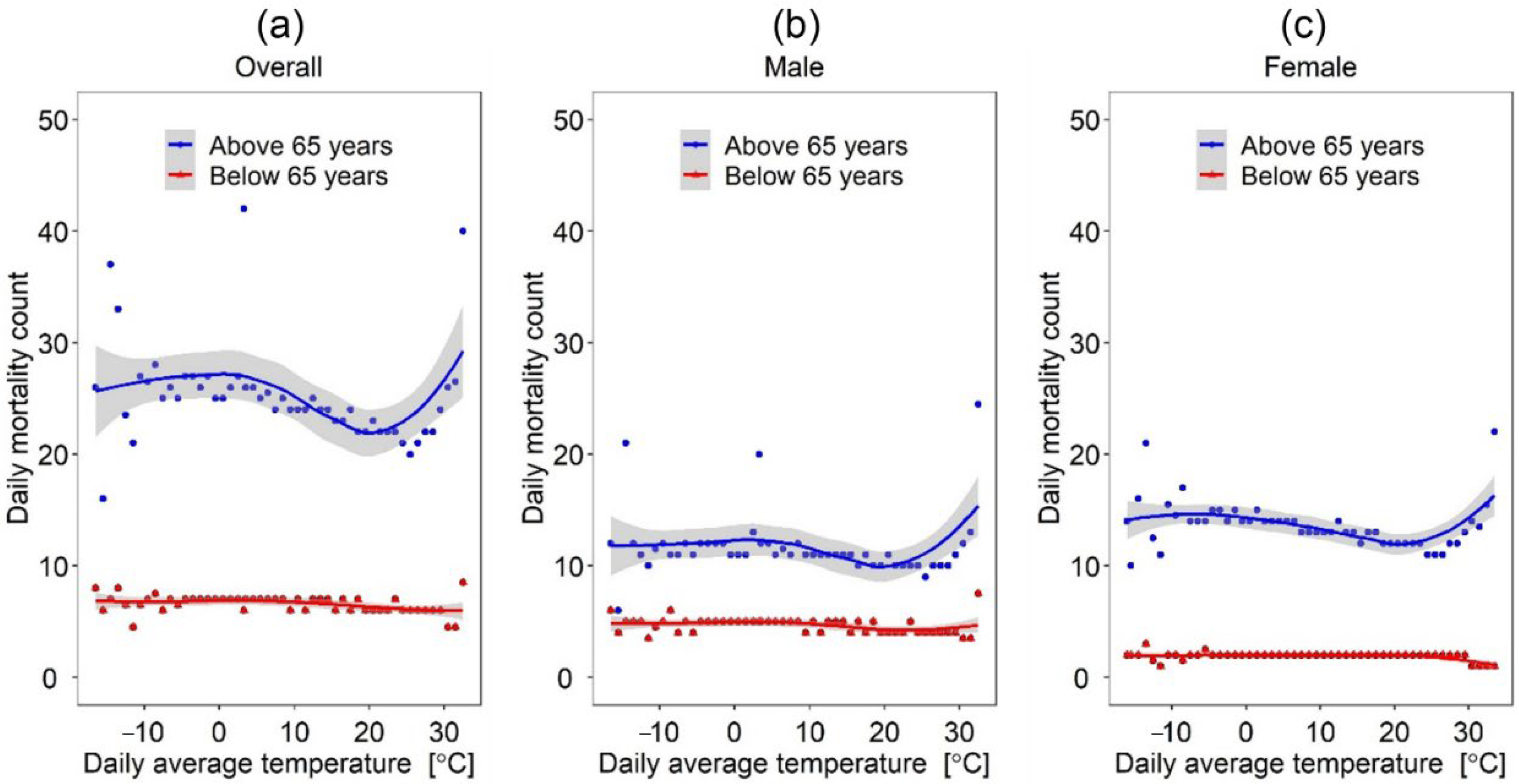
3.3.2. Daily Average Temperature
Figure 5 shows the variations in daily mortality rates as a function of daily average temperature. From the figures, it is apparent that the effect of the daily average temperature on daily mortality is substantially heightened for the “Above 65” age group than the “Below 65” age group. The lowest mortality counts were observed for daily average temperatures slightly lower than 20 °C, and there tends to be a sharp increase in mortality rates at daily average temperatures above 22 °C towards 30 °C. Furthermore, comparing Figure 5b and Figure 5c, the difference in the effect of daily average temperatures on daily mortality counts between genders tended to be negligible.
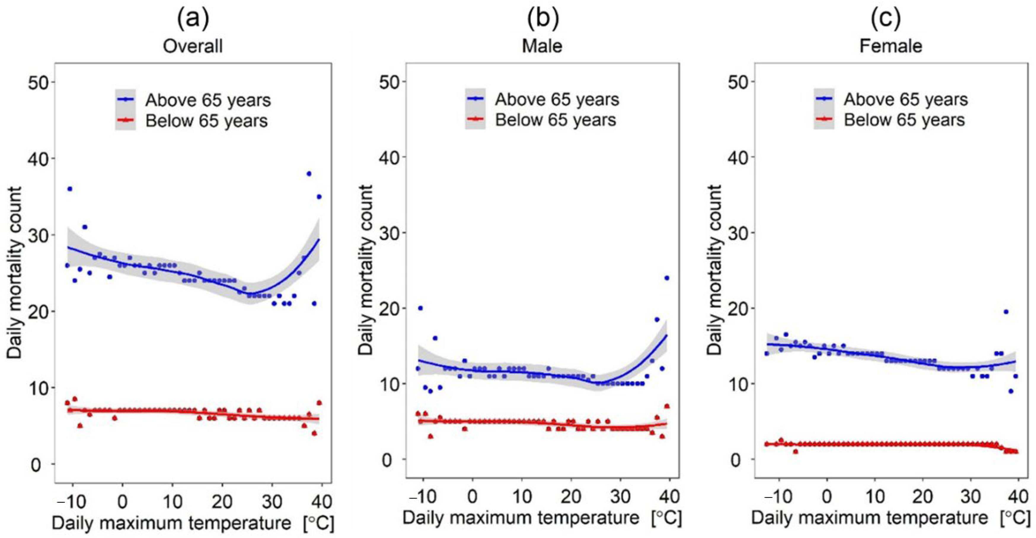
3.3.3. Daily Maximum Temperature
Figure 6 considers the effect of daily maximum temperature on daily mortality counts considering age and gender. Overall, mortalities were relatively high at low daily maximum temperatures but gradually reduced to a minimum at 26.7 °C before sharply increasing again at about 30 °C. Moreover, similar to the previous analysis on the effect of minimum and average daily temperatures on daily mortality counts considering age, there is a more apparent pattern between daily maximum temperature and mortality counts in the “Above 65” age group than the “Below 65” age group. One interesting observation concerns the relationship between daily maximum temperature and female mortality counts; the regression line tended to be relatively flat, indicating no sharp spikes observed at higher temperatures in the male group. This suggests a slightly higher tolerance of heightened temperatures by females than males.
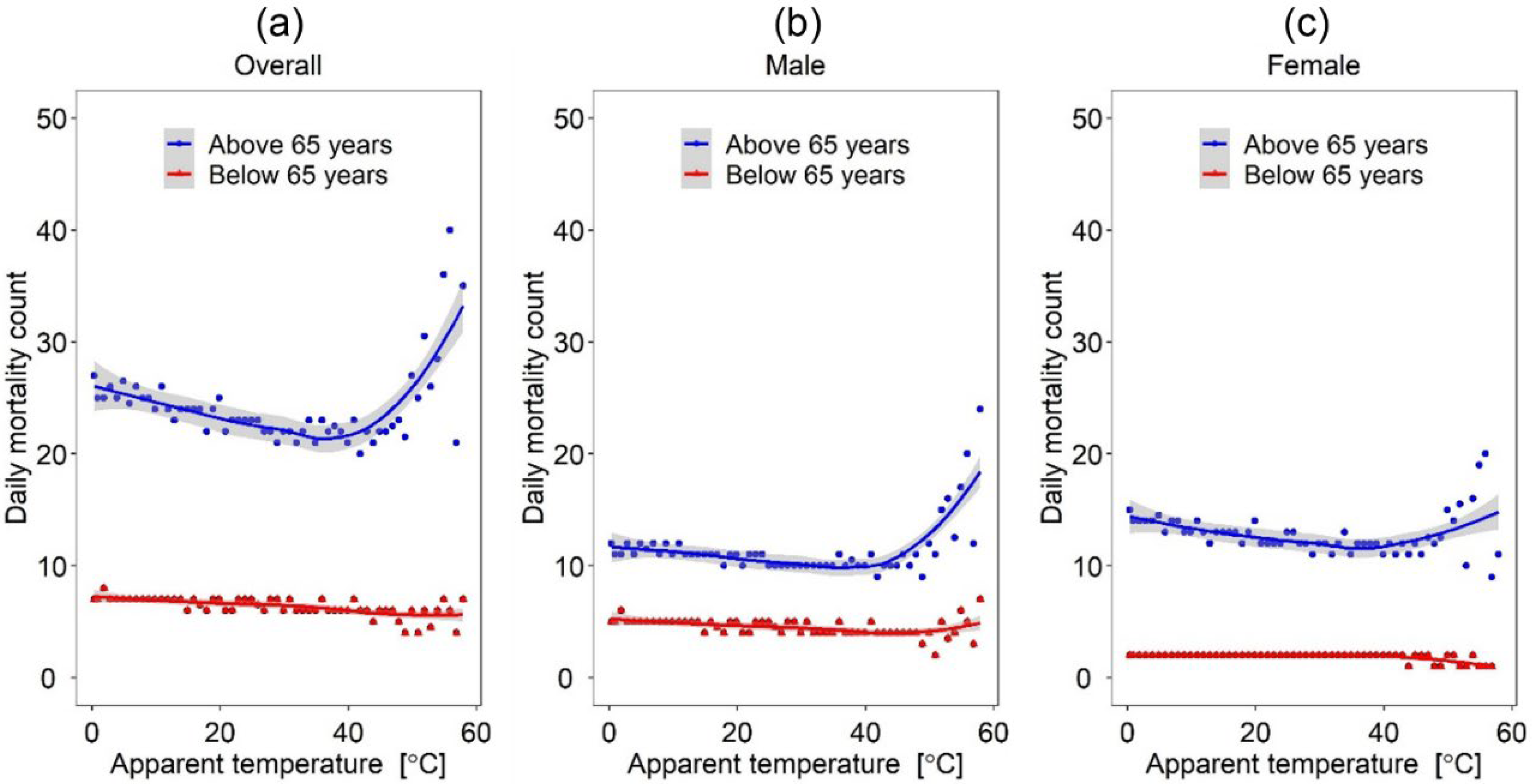
3.3.4. Apparent Temperature
Figure 7 demonstrates the variations in daily mortality counts as a function of apparent temperature. As expected, we observed a U-shaped relationship between apparent temperature and the overall daily mortality counts in the “Above 65” age group. Specifically, high mortality counts at apparent low temperatures gradually decreased to about 40 °C before sharply increasing again. In contrast, the relationship between apparent temperature and the overall daily mortality counts in the “Below 65” age group showed a somewhat flat line indicating no particular influences of apparent temperature. Furthermore, the relationship between apparent temperature and daily mortality counts was more defined for males than females. For instance, there is a much steeper increase in male daily mortality counts (Figure 7b) at apparent temperatures beyond 42 °C compared to female daily mortality counts (Figure 7c).
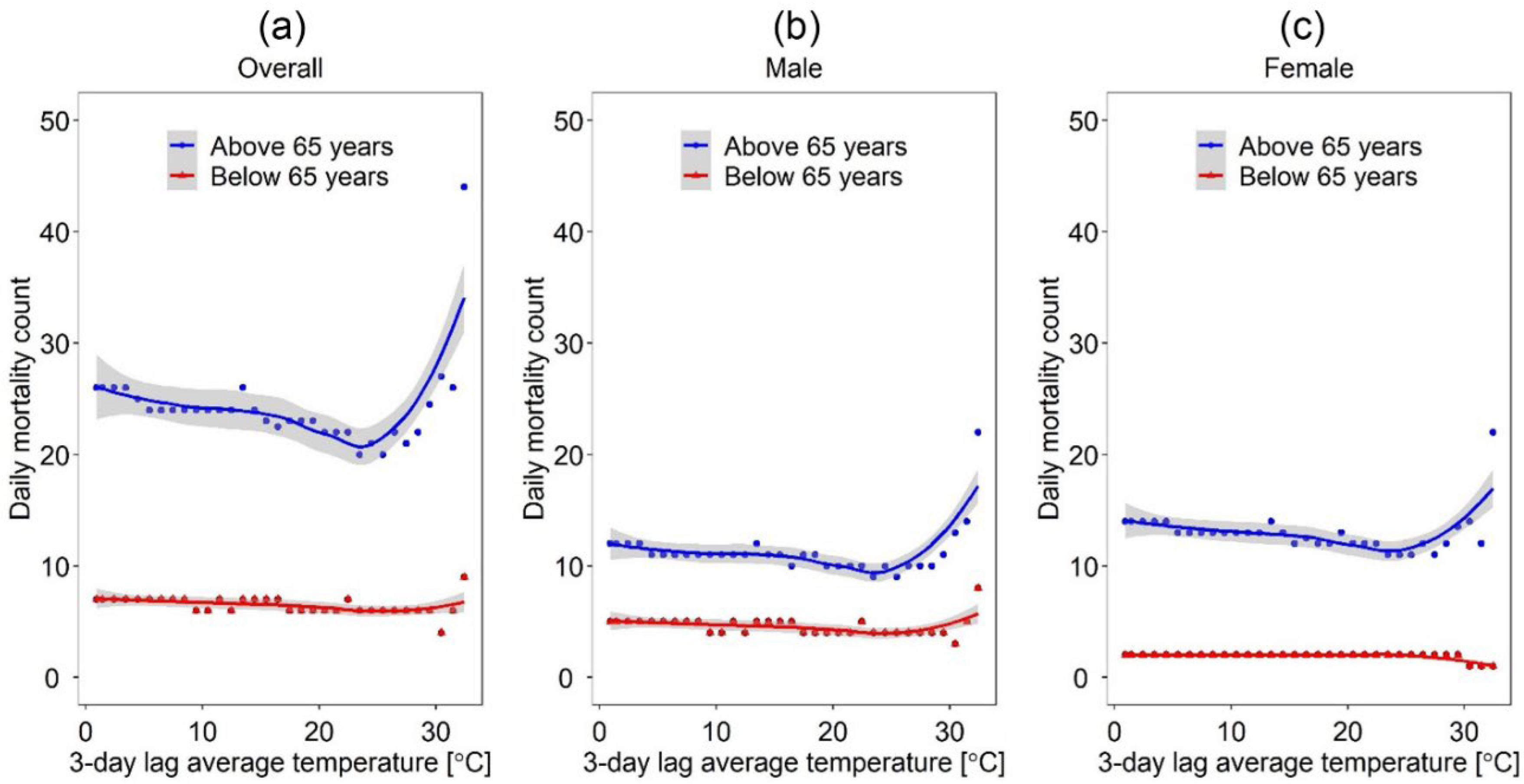
3.3.5. 3-Day Lagged Temperature
Figure 8 shows the relationship of a 3-day lagged temperature on daily mortality counts for each gender and age group. Similar to the previous analysis (shown above), a U-shaped curve, with a sharp increase at a temperature of 22 °C, is observed for the “Above 65” age group while the “Below 65” age group showed rather a flatline. Furthermore, comparing Figure 8b and Figure 8c, we found no substantial differences in the effect of lagged temperature on daily mortalities between genders.
3.4. Potential Effect of HWs on Daily Mortality Counts
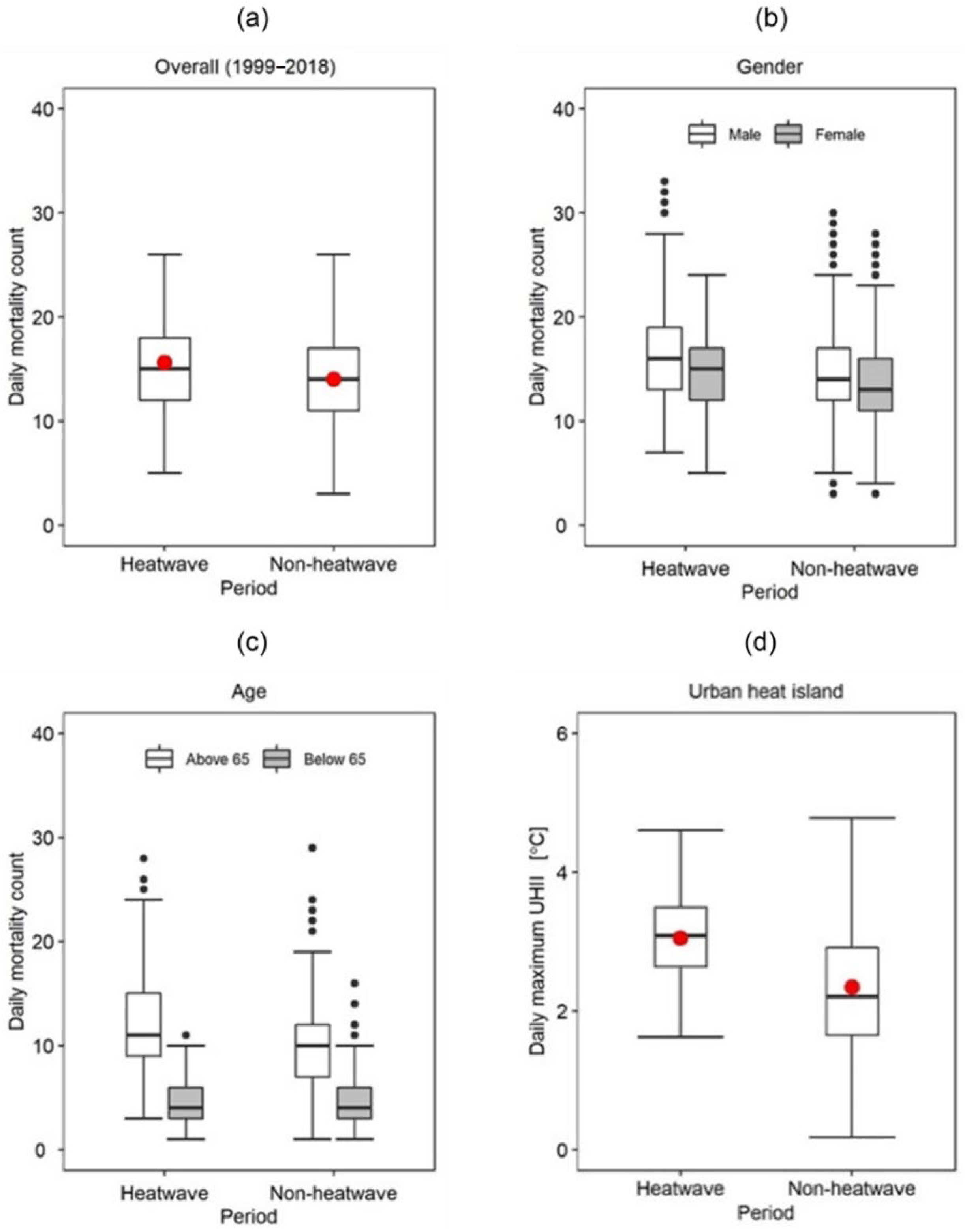
This section considers daily mortality variations during HWs and non-HW (NHW) periods considering gender and age (see Figure 9). Considering the entire period, we observed slightly higher daily mortality counts during HW periods than NHW periods. These differences were also statistically significant, as shown by the ANOVA results in Table 3. The effect of HWs on daily mortality was also observed when considering gender as a modulating factor and was significantly higher for males than females (See Table 4). Similarly, the effect of HWs on daily mortality counts is substantially modulated by age; it is more apparent in the “Above 65” age group and negligible in the “Below 65” age group (See Table 5). UHII was also slightly higher during HW periods than during NHW periods. (See Table 6).
3.5. Potential Effect of UHI on Daily Mortality Count
We considered the potential effect of UHI on mortalities and whether such effects were somewhat modulated by age and season. Table 7 shows correlations between daily average UHI and daily mortality counts. As illustrated in the table, the average daily UHI is more correlated with daily mortalities in the “Above 65” age group than the “Below 65” age group. Taking the overall data (considering the entire period) as an example, our analysis indicates a higher association between UHI, and daily mortality counts in the “above 65” age group (R2 = 0.100) than the “below 65” age group (R2 = 0.003). Furthermore, the observed positive correlations between UHI intensity and mortalities were strongest during the summertime than during other seasons.
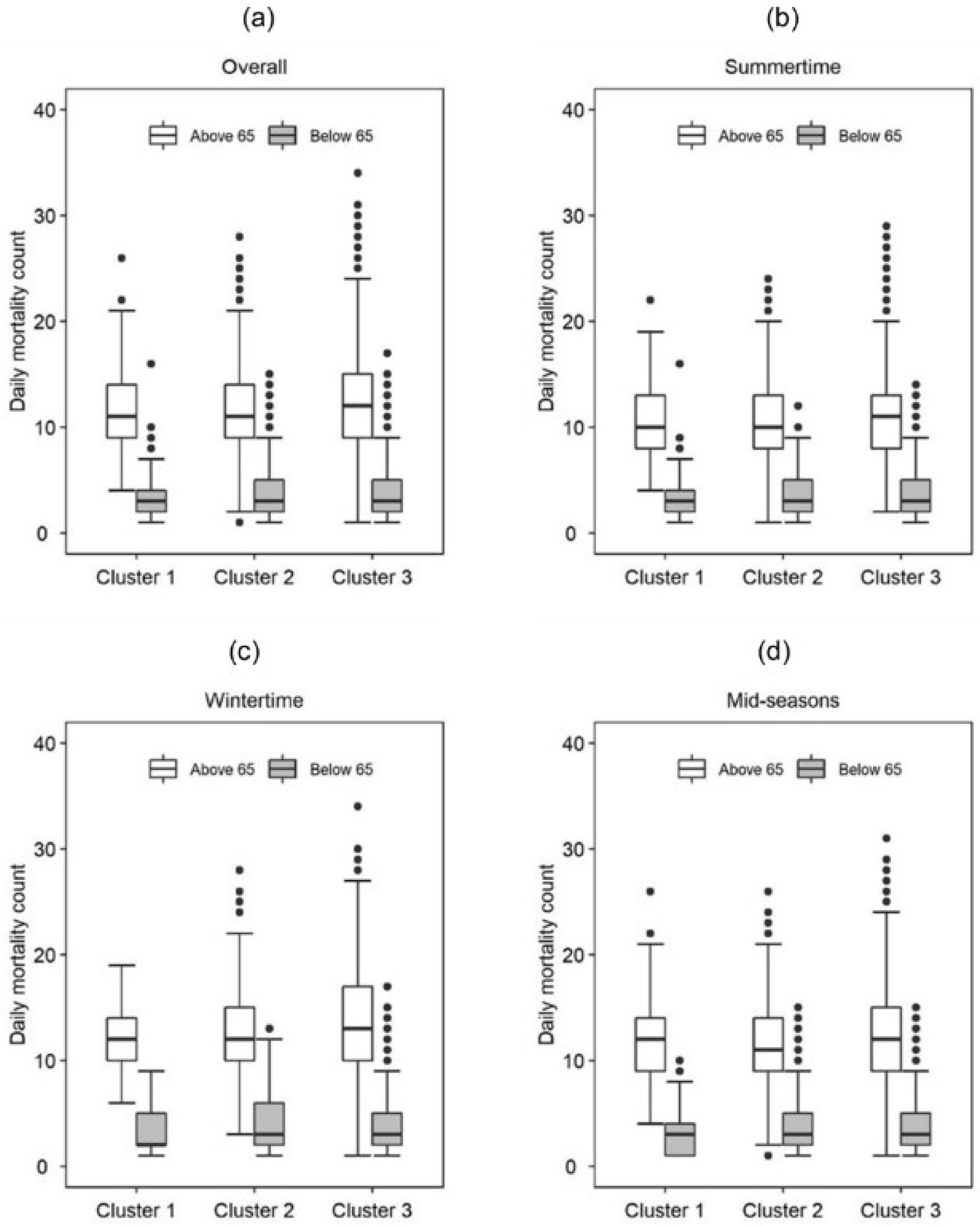
The potential impact of UHI was also analyzed using cluster analysis. As earlier discussed in the methods section, UHI data were grouped into hierarchical clusters of increasing intensities; Low UHI cluster (UHII ≤ 1 °C), medium UHI cluster (1 °C ≤ UHII ≤ 2 °C), and high UHI cluster (UHI > 2 °C). Daily mortality counts were then analyzed across each group while at the same time considering the potential modulating effect of age, gender, and season. Figure 10 shows the variations in daily mortality counts across the three UHI groups for each age group (i.e., Above 65 and Below 65 and across seasons. As seen from the figure, the effect of UHI on daily mortality counts is more apparent in the “Above 65” age group than the “Below 65” age group regardless of the UHI cluster. Taking cluster 1 (i.e., low UHI group) during the summertime as an example, the median difference in daily mortality counts between the “Above 65” and “Below 65” age groups was approximately eight deaths. Relatively similar numbers are seen across the other two clusters regardless of the season.
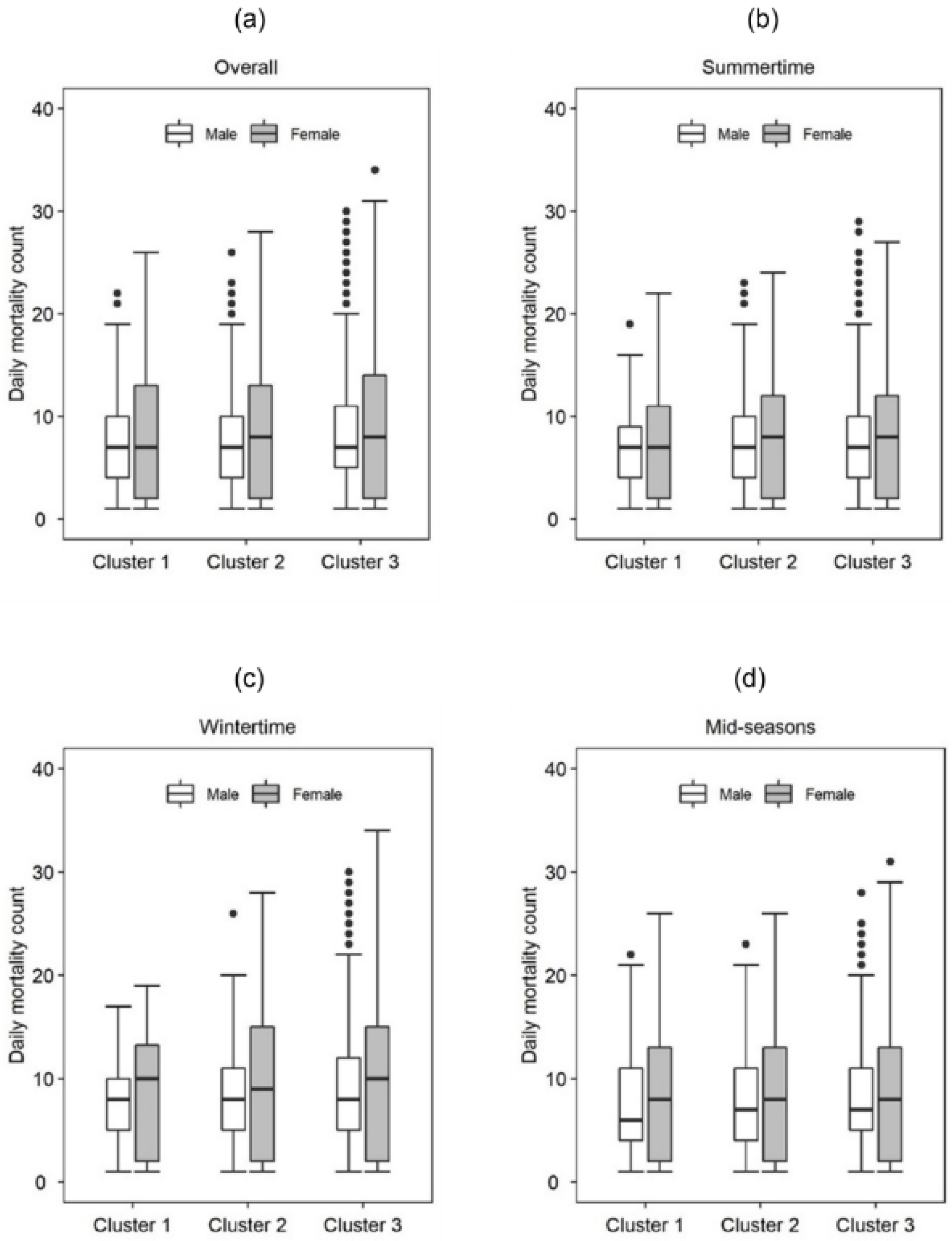
The interactive effect of gender and UHI on daily mortality counts was also analyzed. Figure 11 shows the distributions in daily mortality counts between genders and across different clusters of UHII. As shown in the figure, the differences in daily mortality counts were somewhat the same between the two genders regardless of the UHI cluster. Taking cluster 1 (i.e., low UHI cluster) as an example, it is observed that the difference in median daily mortality counts between genders is negligible. However, the distribution seems much broader for females than males in all seasons.
3.6. Variations in Daily Mortality Counts Considering Education Level and Outdoor Weather
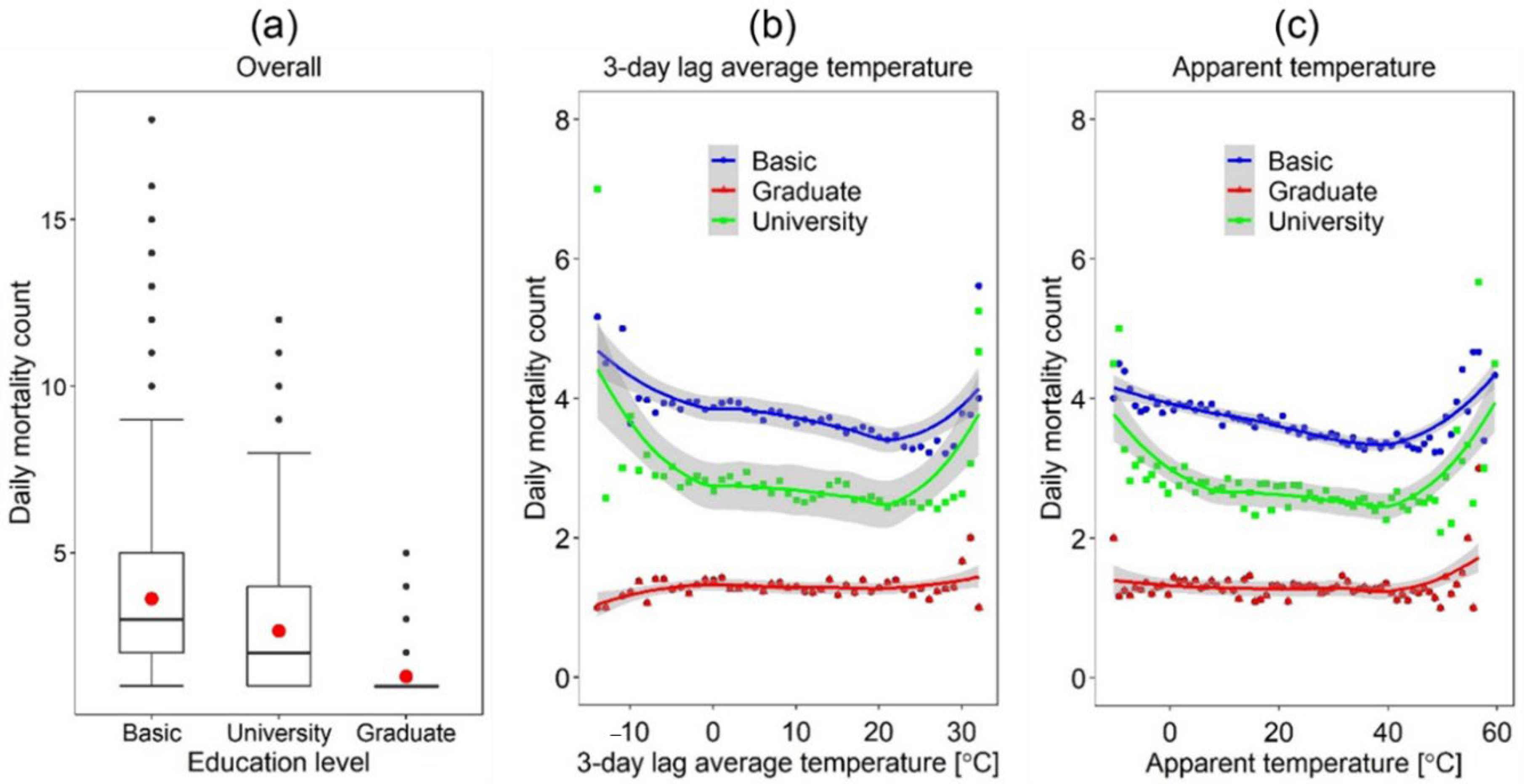
Figure 12 shows the variations of daily mortality counts among groups with different education levels. As indicated in the figure, the highest number of daily mortalities was observed for the low education level group (i.e., Basic). In contrast, the lowest number was observed for the highly educated group (i.e., Graduate school and above). For instance, the median mortality count in the “Basic” education group was 2.5 deaths, while the “Graduate” group was 1 death. This seems to indicate that the higher the education level, the lower the daily mortality counts.
Furthermore, similar results are observed when considering the effect of outdoor weather on the daily mortalities of groups with different education levels. At each given temperature, the daily mortality counts were highest in the low education group (i.e., Basic) and lowest in the high education group (i.e., Graduate). For instance, taking −10 degrees of 3-day lagged temperature as an example, the observed daily mortalities were, 3.9 deaths, 3.6 deaths, and 1.5 deaths for the “Basic”, “University” and “Graduate” education groups, respectively. Similar trends are seen when considering the potential effect of apparent temperature—a higher number of deaths were observed in the low education groups than the high education groups. However, the inflection point upon which heat-related mortalities begin to sharply rise tended to be somewhat the same across the education groups.
3.7. Relative Contributions of Different Factors on Mortality Counts
Table 8 shows the VIF and tolerance values for the considered independent variables. The bolded values show independent variables with potential collinearity issues based on the tolerance and VIF concept. As shown in the table, weather elements constitute substantial collinearity (e.g., VIF values < 10) that might bias the assessment of relative contributions. To assess the relative contributions, therefore, we employed a step-wise regression analysis with (i) time factors, (ii) weather factors, and (iii) personal factors as independent factors. Not all weather elements were introduced, given the observed collinearity. By introducing different variables (i.e., time variables, weather variables, and personal factors) in a step-wise manner, it is observed that personal factors (i.e., gender, age, and education) explain much more of the variance in daily mortality rates than time and weather factors (see Table 9). Note here that adjusted R2 values are presented in addition to R2 values. This is because R2 is a biased estimator when comparing various models; it increases monotonically when new regressors are added to the model even when said regressors have no prognostic addition to the model. As such, to better assess the “value” added by temperature variants (e.g., apparent temperature, maximum UHII) and HWs to Model 2 and later personal factors (e.g., gender, age, and education) in Model 3, adjusted R2 was employed.
3.8. Relative Risk of Mortality
3.8.1. Gender
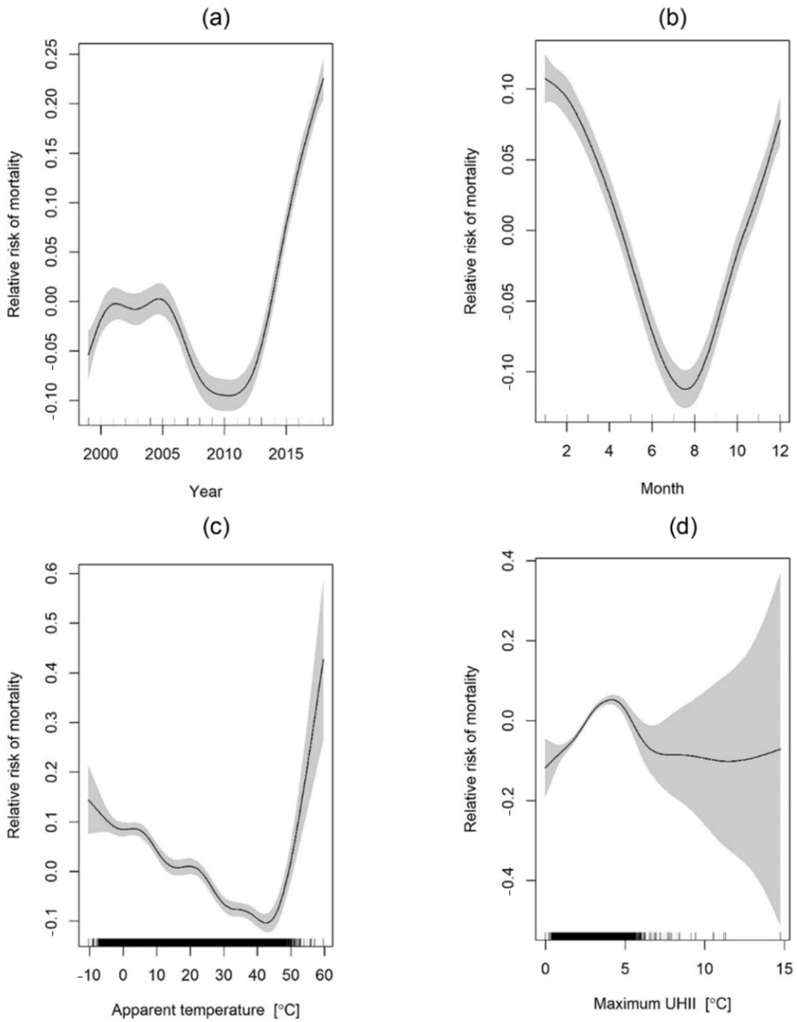
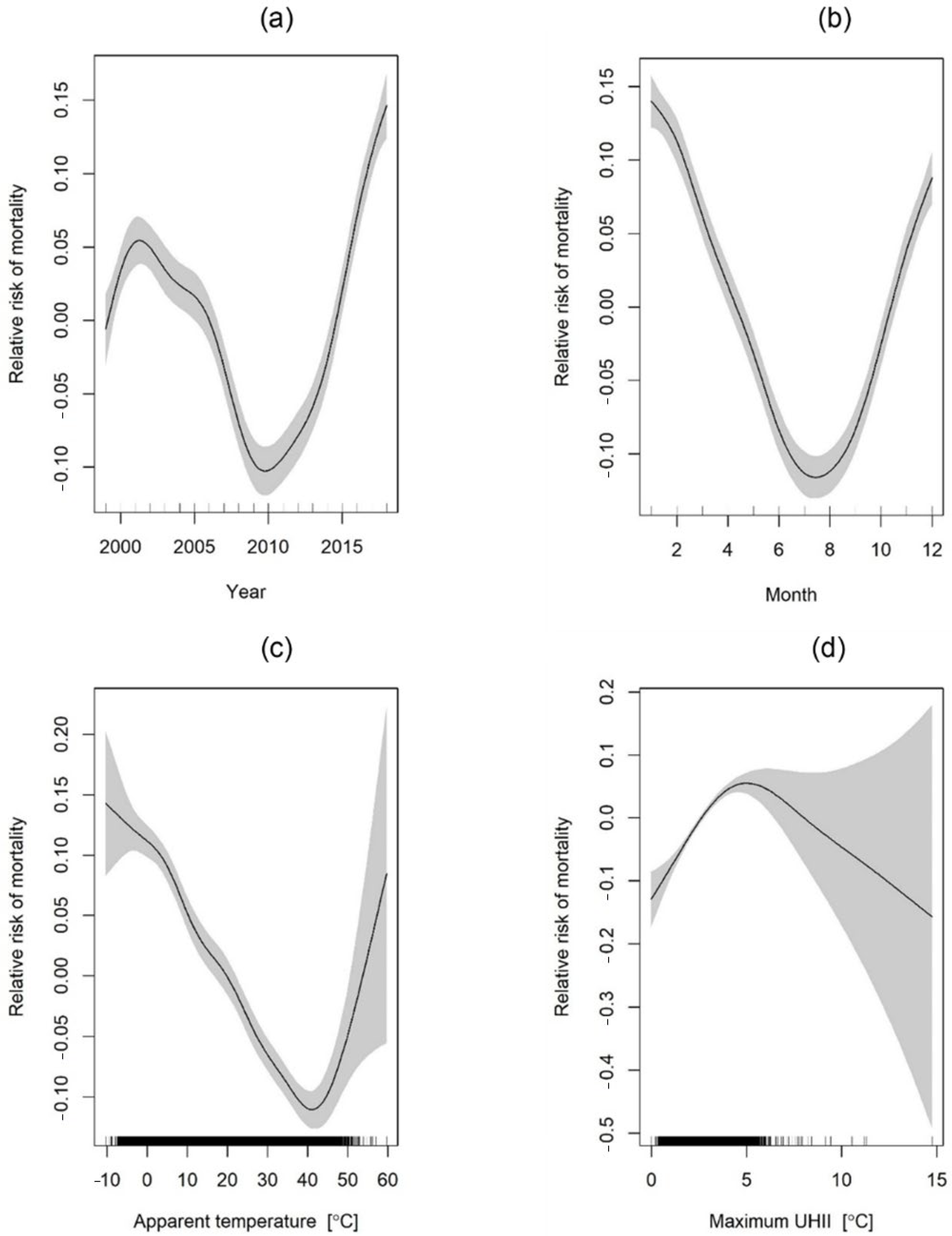
Figure 13 and Figure 14 below indicate estimated relative mortality risk considering gender, time factors, and selected weather factors at a 95% CI. From the figures, it is observed that mortality risk for both males and females increases with increasing years, lowest in the summer period (i.e., July) and highest in the winter period particularly January (RR = 0.10, 95% CI; 0.08–0.12). Furthermore, the relationship between relative mortality risk and apparent temperature shows a U-shaped curve with the lowest risk observed at approximately 40 °C and the highest risk at the highest apparent temperature of approximately 60 °C for both males and females. However, comparing Figure 13c and Figure 14c indicates that relative mortality risks are relatively the same for both genders at low apparent temperatures (RR = 0.10, 95% CI; 0.09–0.20) and slightly more heightened for males (RR = 0.40, 95% CI; 0.23–0.54) than females (RR = 0.05, 95% CI; −0.10–0.20) at higher apparent temperatures (i.e., 60 °C). UHII also tended to be directly proportional to relative risk of mortality for both genders but decreased at UHII above 5 °C (RR = 0.015, 95% CI; 0.012–0.016) perhaps due to the few incidences of UHII above 5 °C. This is also seen from the large margin of errors at UHII above 5 °C (See Figure 13d and Figure 14d).
3.8.2. Age
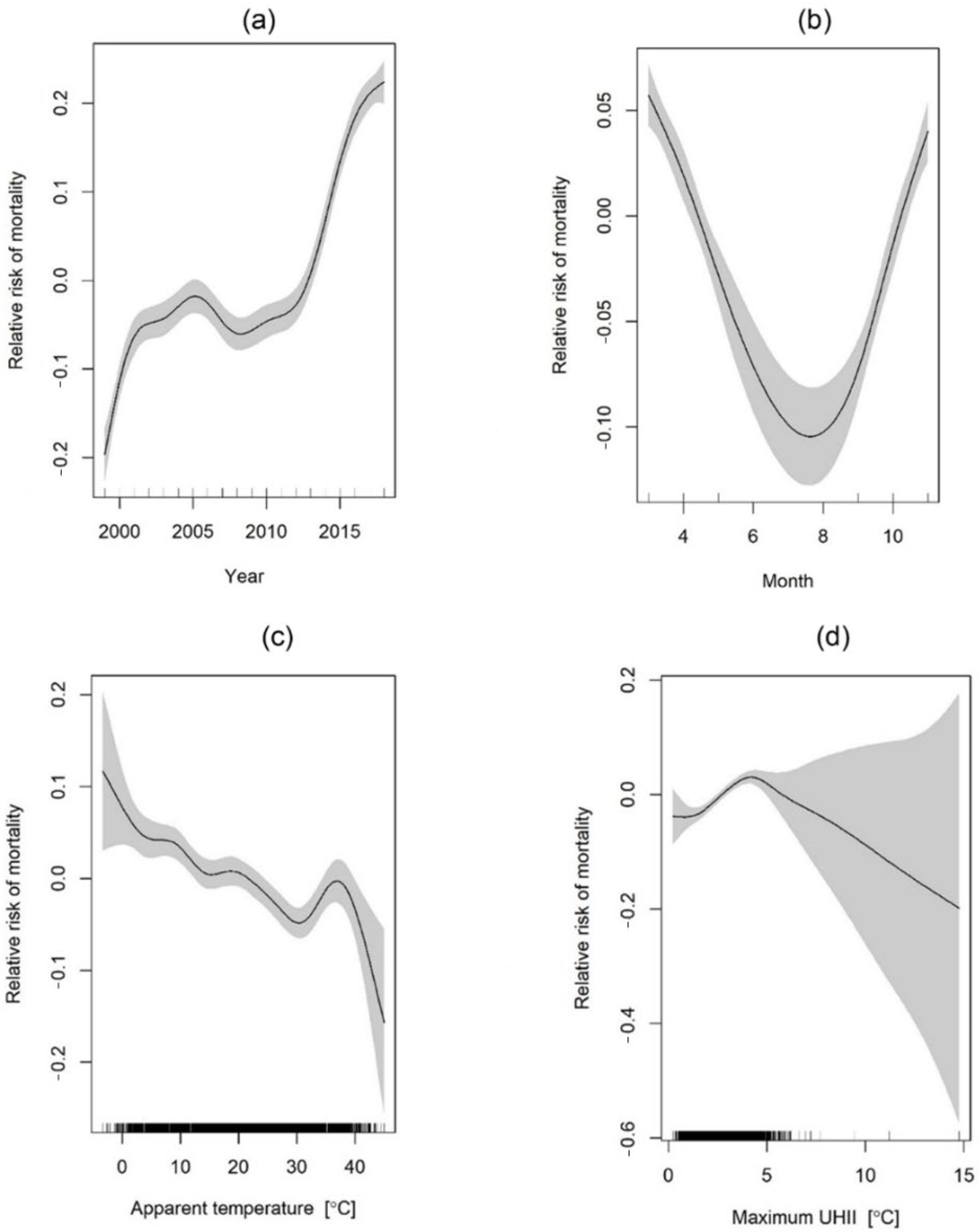
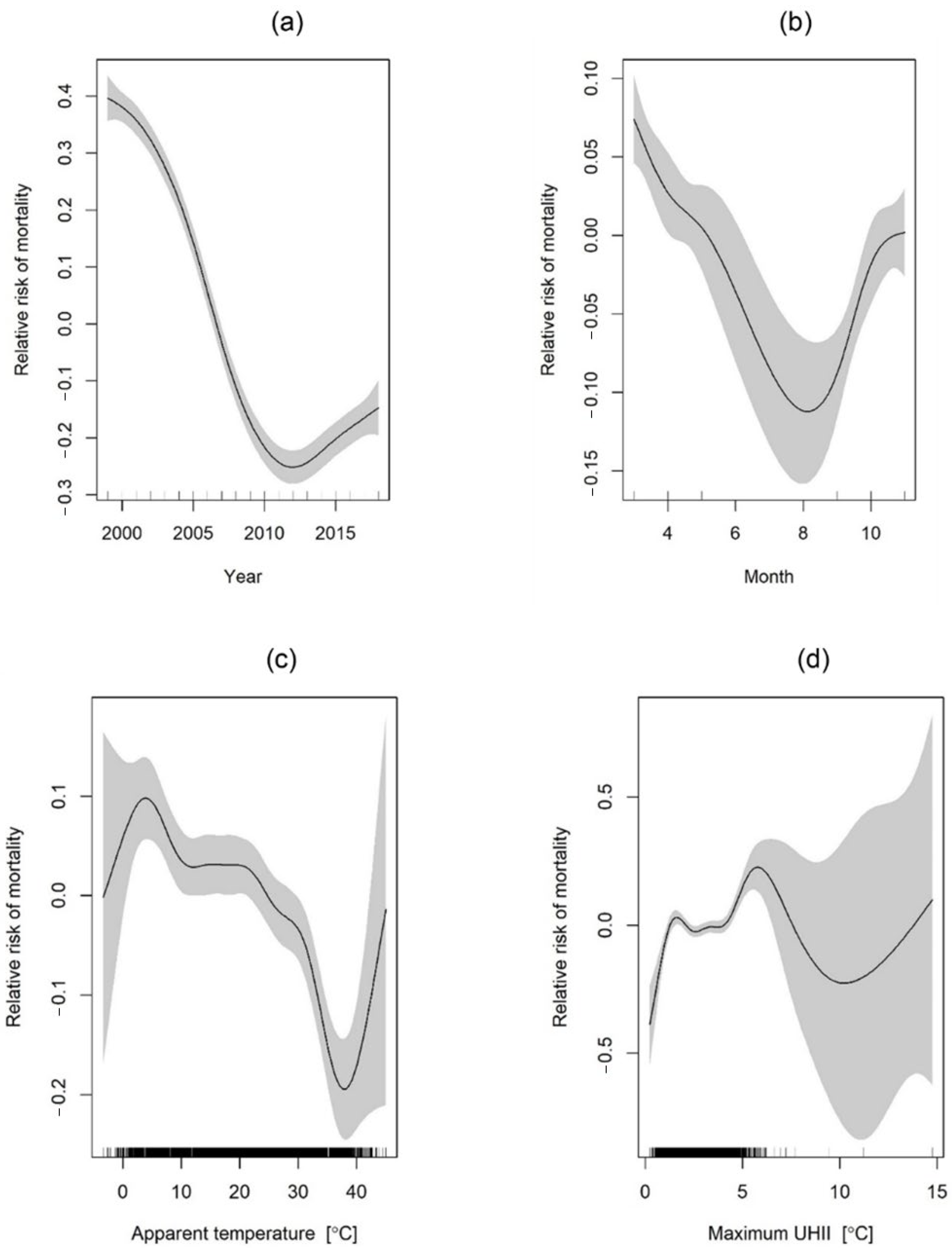
Figure 15 and Figure 16 below indicate estimated relative mortality risk considering age, time factors and selected weather factors. As seen from the figures, we found that the risk of mortality increases with the “Year” factor for the age group above 65 years (Figure 15a) and vice versa for the age group below 65 years (Figure 16a). Moreover, low apparent temperatures were associated with increased mortality risks and the risks were slightly higher for the age group above 65 years (RR = 0.10, 95% CI; 0.002–0.18) than below 65 years (RR = 0.01, 95% CI; −0.1–0.12); similarly, high apparent temperatures are associated with increased mortality risks but the peak apparent temperature upon which mortality risk is highest differs in the two age groups; it is slightly lower for the above 65 age group (38 °C) than the below 65 years age group (>40 °C). UHII is also directly proportional to relative risk of mortality and the induced risk is relatively similar in both age groups (RR = 0.01, 95% CI).
4. Discussion
Climate change, often from the perspective of long-term temporal temperature variability, has been at the forefront of human-centric issues in the 21st century. Epidemiological research, through various methodologies, has shown that extreme temperatures can have diverse physiological strains on a human body, leading to many health issues. For instance, Bobb et al. [56] reported that risks of hospitalization for fluid and electrolyte disorders, renal failure, and urinary tract infection increase under extreme heat events. Similar epidemiological research [57,58,59] has reported the significance of extreme heat vents on people’s physiological well-being, which could eventually lead to fatal outcomes.
The health vulnerabilities imposed by increasing temperatures are a much more severe concern in urban agglomerations as they often experience escalated thermal conditions, mainly resulting from local climate change [25]. While the impacts of temperature changes concern the majority population, the sensitivity and adaptive capacity to said temperature changes vary from demographic to demographic. Such variations are primarily a consequence of a complex combination of personal and social-economic elements. Consequently, it is essential to identify groups most vulnerable to heat exposure and subsequently deliver targeted mitigation and adaptive strategies. Moreover, the compounding effects of local/regional climate change vary from locality to locality and are driven mainly by geographical and social-political-economic elements endemic to said localities. Analyses dealing with the impact of regional and global climate change should thus be area-specific to enable locally tailored interventions and planning. To that end, the main objective of the current study was to quantitively evaluate the associations between temperature and respiratory and cardiovascular mortalities in Seoul while simultaneously analyzing how the said associations differ across different demographics characterized by (i) personal factors (i.e., age and gender), (ii) social-economic factors (i.e., education level), and (ii) local climatic episodes (i.e., UHI and HWs).
Our results showed that the effect of temperature variants (e.g., minimum daily temperature, average daily temperature, and maximum daily temperature) differ significantly across different age groups (i.e., above 65 years and below 65 years of age) and between males and females. For instance, given the same daily maximum temperature, the number of mortalities was significantly higher for females above 65 years of age than their male counterparts (see Figure 6). The finding reports that older females are more vulnerable to health issues resulting from elevated temperatures and reiterates reports from studies in South Korea [60], Spain [61], England [62] as well as cities in China [63]. Such differences in sensitivities to heat exposure between genders are, to an extent, attributed to differences in physiological characteristics inherent of the two genders (e.g., in terms of temperature regulatory mechanisms [64,65]. Another possible explanation for such a result pertains to social demographic characteristics that encourage gender differences in elements such as life expectancy and social isolation [61,66]. On the contrary, a study conducted in the Tibetan counties in China reported males to be more susceptible to extreme temperature exposure than females [67]. Similarly, a recent study conducted in multiple cities in China found that males were more affected by high-frequency temperature variations than females [68] while another study in Taiwan found no differences in susceptibility between the two genders [69]. Such observations seem to emphasize regional differences in temperature-mortality effects and perhaps warrants more intense discussions on the role of regional climatic conditions on temperature-mortality relationships.
One interesting finding with vast implications for urban planning policies is the inflection temperature point upon which daily mortalities increase between the two genders. This is better observed considering the daily average temperature (see Figure 5)—the inflection temperature point for males was observed at 20 °C while that for females was 21.5 °C. The finding suggests that the population in Seoul is acclimatized to low temperatures and that this is more the case for males than females. This can also be viewed from the perspective of physiological differences between the two sexes; men have been reported to have larger decreases in core body temperature than women when exposed to cold temperatures [70], and possibly the reason for the observed lower inflection temperature point in males than females (i.e., 20 °C vs. 21.5 °C).
Furthermore, age was indicated as a significant factor contributing to heat-related mortalities. For instance, given the same outdoor temperature conditions, the number of mortalities was significantly higher for the “above 65 years” age group than the “below 65 years” age group. This finding also corroborates reports from previous studies [52] and is potentially explained by the age-related differences in physiological mechanisms that influence thermoregulatory pathways. For instance, during elevated heat exposure, older individuals are reported to respond with reduced blood flow from the skin and minimized redistribution of blood from the splanchnic and renal circulations relative to younger individuals—as a result, core body temperatures increase, potentially leading to hypothermia [71].
Low-educated groups showed higher mortalities than high-educated groups. We hypothesize that the primary reasons for the seen differences in heat-related mortalities among groups with different education levels are closely linked to occupational job differences and long-term differences in financial capabilities. For instance, individuals in the high education clusters are likely involved in professions often conducted in well-ventilated/heated indoor spaces, significantly reducing the toll of temperature extremes on their health; the opposite is likely true for individuals in low education clusters. Additionally, other lifestyle differences that arise from the variability in economic status between highly educated and low-educated individuals (e.g., quality of their homes, access to a nutritious diet, access to medical facilities) and that lead to accumulated health issues in the low-education group—these pre-existing issues could exacerbate the influence of extreme temperature deviations on low educated individuals leading to increased rates of mortality.
Our analysis also showed that, generally, heat-related daily mortalities were on average 1 death higher during HW than NHW periods. Such findings are commensurate with reports from previous studies; For example, a study on non-accidental deaths during HWs in European cities reported increases in HW-induced mortalities of up to 33.6% in Milan and 7.6% in Munich [72]. The effect of HWs on heat-related mortalities is fundamentally explained by the earlier discussed severe pressure that heat exposure exerts on the thermoregulatory mechanisms of the human body. One specifically interesting observation relates to how gender modulates the influence of HWs on heat-related mortality. For example, we found that the number of heat-related deaths during HW was, on average, two deaths higher in males than females (see Table 4). This finding corroborates recent observations in Seoul that report a slightly higher risk of male mortality than female mortality during HW episodes [73]. However, numerous other studies have reported contradictory observations. For example, Fouillet et al., [74], reported a higher percentage (i.e., 64%) of female deaths than male deaths during the 2003 HW in France. Similar reports have been observed in Chinese cities [75] and more recently in Senegal [76]. One potential reason for the contradictions in the literature is perhaps because a vast number of previous research have seldom considered other demographic characteristics likely to expose men more to heat risks, particularly during HW episodes. For instance, outdoor workers who consist mainly of a higher proportion of men than women are particularly vulnerable to exertional heat strokes stemming from elevated temperatures during HW episodes. Consequently, it is essential to analyze the effects of gender on heat-related mortalities during HW episodes for specific subgroups. Additionally, assessing the role of public health interventions and the implementation of early warning systems for extreme heat events on reducing heat-related mortalities would provide deeper insights on the real effect of HWs on temperature-related deaths. This would be particularly interesting as recent studies in South Korea [77] have reported a relatively higher number of HW-related deaths in rural areas than urban areas. While such observations contradict existing theoretical evidence, they also point to the lack of in-depth analysis on the impact of HW on temperature-related mortalities that considers other overlooked social-economic characteristics such as the prevalence of HVAC usage and availability in the much-developed sub-regions of Seoul city. The observed effect of HWs on mortality is also potentially amplified by the additional influence of UHI. Previous studies [20,22,78] have drawn linkages between HW and UHI, illustrating synergetic interactions between the two elements. These interactions are also found in the present study (See Figure 9) and further point to the usefulness of UHI mitigative measures in reducing mortalities during HWs.
We also assessed the potential effect of UHI on heat-related mortalities across sexes and age groups. Our results showed that the number of heat-related mortalities was significantly higher in high UHII clusters than low UHII clusters, particularly for the “above 65” age group and the females, further pointing to the attenuated sensitivity to heat exposure by females and the elderly. It is worth noting that the direct influences of UHI on heat-related mortality have been somewhat neglected in the literature despite its obvious significance for climate-resilient environments [79] and adaptive potential that can be achieved through implementing UHI mitigative strategies [80]. Studies that precisely assess the effect of UHI on heat-related mortality are warranted and critical in the development of robust urban health policies. Furthermore, it is worth noting that although the models relating UHII to seasonal mortality explain relatively low mortality variations (see Table 7), the models are still statistically significant at a p-value < 0.05, indicating a good fit of the model to the data. Perhaps increasing the amount of data could better establish the inferred relationship between UHI intensity and mortality in Seoul—this is one issue that can be looked into as large datasets covering long periods become available.
Our results also reiterate previous reports on the impact of seasonality on temperature-related mortalities [81]. The mortality risk is substantially lower during the summer months than in winter, which points to a more serious concern for cold-related mortalities than heat-related mortalities in Seoul, especially for females and the elderly (e.g., >65 years of age). One potential reason for the higher mortalities during cold periods is linked to bronchoconstriction likely to develop during exposure to extreme cold conditions. Cold exposure also weakens mucociliary defenses, which cause respiratory infections and potential inflammation [82]. These conditions are likely to persist longer than those caused by heat exposure. They have been reported as the potential reason for the higher mortalities during colder periods than hotter ones [83]. This observation has wide implications, particularly regarding the current research trends in the field. Most of the research in the field seems to focus more on the consequences of heat-related mortalities, yet cold exposure claims higher mortality counts. Our findings agree with those by Gasparrini et al. [84], who critically reviewed existing epidemiological studies and found higher mortalities associated with cold exposure than heat exposure. This observation is useful for public health policies, particularly for Seoul city, as it evidences the mortality risk associated with cold exposure and provides a platform for discussing relevant policies and mitigation strategies. Moreover, while our results show a decline in the risk of temperature-related mortalities over the years for the “below 65 age group” (see Figure 16a), the risk increased substantially for the “above 65 age group” (see Figure 15a). This finding partly contradicts previous observations [85] reporting a temporal decline in heat-related mortalities during summers in South Korea and cold-related mortalities in London [86]. The contradictions are, potentially, because studies in the field have often concentrated on different demographics with no agreed-upon categorization scheme. For instance, the definition for elderly individuals seems to lack consistency across studies in the literature. Moreover, the role of improved infrastructure, technology, and public health interventions is seldom incorporated into the analysis. With such uncertainties, understanding the effect of temperature on human health becomes even more challenging. There is thus abundant space for analyzing temporal trends in temperature-related mortality in Seoul, particularly considering other social-economic elements (e.g., prevalence and use of aiding mechanical equipment) and newly implemented urban policies.
5. Conclusions
We set out to determine associations between temperature changes, HWs, and UHI on respiratory and cardiovascular mortalities in Seoul for a period of 19 years (1999–2018). At the same time, we observed how the said associations varied across different demographics characterized by personal and social-economic factors (e.g., age, gender, and education level). Additionally, through GAM regression, we estimated the relative risk of mortality induced by temperature changes for different demographic groups. We found that temperature-related risk of mortality in Seoul has increased after 2010 for both men and women and particularly for older individuals (i.e., above 65 years of age); the risk of mortality was slightly lower for younger individuals (i.e., below 65 years of age). In addition, among the many variants of temperature considered, the apparent temperature is mostly correlated to daily mortalities in Seoul; this relationship is substantially modulated by age while gender plays a very slight role. We also found that HW episodes had a more substantial impact on males than females. The effect of UHI on temperature-related mortalities was more apparent during the summertime than in other seasons. The observations pinpoint the cofounding effects of social-economic elements on temperature–mortality relations and help identify groups most vulnerable to regional temperature changes. Moreover, they provide key insights useful in developing urban health policies that promote climate resilience and adaptation.
6. Limitations and Future Research
The present article faces a few limitations. One such limitation is related to the heat stress measurement indices used in the study. For instance, we considered several variants of air temperature, particularly apparent temperature, which captures the integrated toll that air temperature and humidity have on heat stress. Similarly, we used absolute air temperature values. However, these indices do not consider certain critical elements, such as radiation and convective air flows, that have a substantial influence on the thermal load experienced by a subject. Consequently, future research needs to consider indices incorporating other essential factors likely to affect thermal stress on the human body. It is also important to note that there is a plethora of factors likely to compound the impact of thermal changes on human health and which were not considered in the present study. For instance, the present article did not control for the potential impact of the synergetic interactions between urban pollution and urban warming on mortality despite its likely huge effect on temperature-related mortality. Additionally, the quality of built environments (e.g., homes, offices) in terms of thermal insulation and access to cooling equipment substantially affects how individuals cope with heat stress and is an essential factor in assessing heat-related mortality. There are also factors related to the physical activeness of the deceased. Individuals with active physical lifestyles are likely to suffer fewer heat-related incidents, which perhaps explains increased heat-related mortalities in old individuals. Consequently, considering all these factors could indeed further our understanding of heat-related mortalities and underlying factors.
Author Contributions
Conceptualization, J.N., G.Y.Y. and M.S.; methodology, J.N., G.Y.Y. and M.S.; formal analysis, J.N., G.Y.Y. and M.S.; resources, G.Y.Y.; data curation, J.N.; writing—original draft preparation, J.N., G.Y.Y. and M.S.; writing—review and editing, J.N., G.Y.Y. and M.S.; visualization, J.N., G.Y.Y. and M.S.; funding acquisition, G.Y.Y. All authors have read and agreed to the published version of the manuscript.
Funding
This work was supported by the National Research Foundation of Korea (NRF) grant funded by the Korea government (MSIT) (No. 2020R1A2C1099611).
Institutional Review Board Statement
Not applicable.
Informed Consent Statement
Not applicable.
Data Availability Statement
The data maybe provided upon reasonable request from the corresponding author.
Conflicts of Interest
The authors declare no conflict of interest. The funders had no role in the design of the study; in the collection, analyses, or interpretation of data; in the writing of the manuscript; or in the decision to publish the results.
Abbreviations
| HW | Heat waves |
| NHW | Non-heat waves |
| UHI | Urban heat island |
| UHII | Urban heat island intensity |
| KMA | Korea meteorological agency |
| AWS | Automatic weather station |
| WMO | World meteorological organization |
| VIF | Value inflation factor |
| GAM | Generalized additive models |
| RR | Relative ratio |
| HVAC | Heating ventilation and air conditioning |
References
- Sweileh, W.M. Bibliometric Analysis of Peer-Reviewed Literature on Climate Change and Human Health with an Emphasis on Infectious Diseases. Global. Health 2020, 16, 1–17. [Google Scholar] [CrossRef] [PubMed]
- Vicedo-Cabrera, A.M.; Scovronick, N.; Sera, F.; Royé, D.; Schneider, R.; Tobias, A.; Astrom, C.; Guo, Y.; Honda, Y.; Hondula, D.M.; et al. The Burden of Heat-Related Mortality Attributable to Recent Human-Induced Climate Change. Nat. Clim. Chang. 2021, 11, 492–500. [Google Scholar] [CrossRef] [PubMed]
- Zafeiratou, S.; Samoli, E.; Dimakopoulou, K.; Rodopoulou, S.; Analitis, A.; Gasparrini, A.; Stafoggia, M.; De’ Donato, F.; Rao, S.; Monteiro, A.; et al. A Systematic Review on the Association between Total and Cardiopulmonary Mortality/Morbidity or Cardiovascular Risk Factors with Long-Term Exposure to Increased or Decreased Ambient Temperature. Sci. Total Environ. 2021, 772, 145383. [Google Scholar] [CrossRef]
- Liu, J.; Hansen, A.; Varghese, B.; Liu, Z.; Tong, M.; Qiu, H.; Tian, L.; Lau, K.K.L.; Ng, E.; Ren, C.; et al. Cause-Specific Mortality Attributable to Cold and Hot Ambient Temperatures in Hong Kong: A Time-Series Study, 2006–2016. Sustain. Cities Soc. 2020, 57, 102131. [Google Scholar] [CrossRef]
- Gasparrini, A.; Guo, Y.; Sera, F.; Vicedo-Cabrera, A.M.; Huber, V.; Tong, S.; de Sousa Zanotti Stagliorio Coelho, M.; Nascimento Saldiva, P.H.; Lavigne, E.; Matus Correa, P.; et al. Projections of Temperature-Related Excess Mortality under Climate Change Scenarios. Lancet Planet. Health 2017, 1, e360–e367. [Google Scholar] [CrossRef]
- Basarin, B.; Lukić, T.; Matzarakis, A. Review of Biometeorology of Heatwaves and Warm Extremes in Europe. Atmosphere 2020, 11, 1276. [Google Scholar] [CrossRef]
- Robine, J.M.; Cheung, S.L.K.; Le Roy, S.; Van Oyen, H.; Griffiths, C.; Michel, J.P.; Herrmann, F.R. Death Toll Exceeded 70,000 in Europe during the Summer of 2003. Comptes Rendus Biol. 2008, 331, 171–178. [Google Scholar] [CrossRef] [PubMed]
- Sahani, J.; Kumar, P.; Debele, S.; Emmanuel, R. Heat Risk of Mortality in Two Different Regions of the United Kingdom. Sustain. Cities Soc. 2022, 80, 103758. [Google Scholar] [CrossRef]
- Ostro, B.D.; Roth, L.A.; Green, R.S.; Basu, R. Estimating the Mortality Effect of the July 2006 California Heat Wave. Environ. Res. 2009, 109, 614–619. [Google Scholar] [CrossRef]
- Barriopedro, D.; Fischer, E.M.; Luterbacher, J.; Trigo, R.M.; García-Herrera, R. The Hot Summer of 2010: Redrawing the Temperature Record Map of Europe. Science 2011, 332, 220–224. [Google Scholar] [CrossRef]
- Choi, N.; Lee, M.I. Spatial Variability and Long-Term Trend in the Occurrence Frequency of Heatwave and Tropical Night in Korea. Asia-Pac. J. Atmos. Sci. 2019, 55, 101–114. [Google Scholar] [CrossRef]
- Oke, T.R. The Energetic Basis of the Urban Heat Island. Q. J. R. Meteorol. Soc. 1982, 108, 1–24. [Google Scholar] [CrossRef]
- Ngarambe, J.; Oh, J.W.; Su, M.A.; Santamouris, M.; Yun, G.Y. Influences of Wind Speed, Sky Conditions, Land Use and Land Cover Characteristics on the Magnitude of the Urban Heat Island in Seoul: An Exploratory Analysis. Sustain. Cities Soc. 2021, 71, 102953. [Google Scholar] [CrossRef]
- Li, Y.; Sun, Y.; Li, J.; Gao, C. Socioeconomic Drivers of Urban Heat Island Effect: Empirical Evidence from Major Chinese Cities. Sustain. Cities Soc. 2020, 63, 102425. [Google Scholar] [CrossRef]
- Lowe, S.A. An Energy and Mortality Impact Assessment of the Urban Heat Island in the US. Environ. Impact Assess. Rev. 2016, 56, 139–144. [Google Scholar] [CrossRef]
- Paravantis, J.; Santamouris, M.; Cartalis, C.; Efthymiou, C.; Kontoulis, N. Mortality Associated with High Ambient Temperatures, Heatwaves, and the Urban Heat Island in Athens, Greece. Sustainability 2017, 9, 606. [Google Scholar] [CrossRef] [Green Version]
- Taylor, J.; Wilkinson, P.; Davies, M.; Armstrong, B.; Chalabi, Z.; Mavrogianni, A.; Symonds, P.; Oikonomou, E.; Bohnenstengel, S.I. Mapping the Effects of Urban Heat Island, Housing, and Age on Excess Heat-Related Mortality in London. Urban Clim. 2015, 14, 517–528. [Google Scholar] [CrossRef]
- Tan, J.; Zheng, Y.; Tang, X.; Guo, C.; Li, L.; Song, G.; Zhen, X.; Yuan, D.; Kalkstein, A.J.; Li, F.; et al. The Urban Heat Island and Its Impact on Heat Waves and Human Health in Shanghai. Int. J. Biometeorol. 2010, 54, 75–84. [Google Scholar] [CrossRef]
- Wu, S.; Wang, P.; Tong, X.; Tian, H.; Zhao, Y.; Luo, M. Urbanization-Driven Increases in Summertime Compound Heat Extremes across China. Sci. Total Environ. 2021, 799, 149166. [Google Scholar] [CrossRef]
- Founda, D.; Santamouris, M. Synergies between Urban Heat Island and Heat Waves in Athens (Greece), during an Extremely Hot Summer (2012). Sci. Rep. 2017, 7, 1–11. [Google Scholar] [CrossRef]
- Khan, H.S.; Paolini, R.; Santamouris, M.; Caccetta, P. Exploring the Synergies between Urban Overheating and Heatwaves (HWS) in Western Sydney. Energies 2020, 13, 470. [Google Scholar] [CrossRef] [Green Version]
- Ngarambe, J.; Nganyiyimana, J.; Kim, I.; Santamouris, M.; Young Yun, G. Synergies between Urban Heat Island and Heat Waves in Seoul: The Role of Wind Speed and Land Use Characteristics. PLoS ONE 2020, 15, e0243571. [Google Scholar] [CrossRef]
- Miao, S.; Zhan, W.; Lai, J.; Li, L.; Du, H.; Wang, C.; Wang, C.; Li, J.; Huang, F.; Liu, Z.; et al. Heat Wave-Induced Augmentation of Surface Urban Heat Islands Strongly Regulated by Rural Background. Sustain. Cities Soc. 2022, 82, 103874. [Google Scholar] [CrossRef]
- Zhang, Y.; Mao, G.; Chen, C.; Lu, Z.; Luo, Z.; Zhou, W. Population Exposure to Concurrent Daytime and Nighttime Heatwaves in Huai River Basin, China. Sustain. Cities Soc. 2020, 61, 102309. [Google Scholar] [CrossRef]
- Nazarian, N.; Krayenhoff, E.S.; Bechtel, B.; Hondula, D.; Paolini, R.; Vanos, J.; Cheung, T.; Chow, W.T.L.; de Dear, R.; Lee, J.K.W.; et al. Integrated Assessment of Urban Overheating Impacts on Human Life. Earths Future 2022, 10, e2022EF002682. [Google Scholar] [CrossRef]
- Botzen, W.J.W.; Martinius, M.L.; Bröde, P.; Folkerts, M.A.; Ignjacevic, P.; Estrada, F.; Harmsen, C.N.; Daanen, H.A.M. Economic Valuation of Climate Change–Induced Mortality: Age Dependent Cold and Heat Mortality in the Netherlands. Clim. Chang. 2020, 162, 545–562. [Google Scholar] [CrossRef]
- Alele, F.; Malau-Aduli, B.; Malau-Aduli, A.; Crowe, M. Systematic Review of Gender Differences in the Epidemiology and Risk Factors of Exertional Heat Illness and Heat Tolerance in the Armed Forces. BMJ Open 2020, 10, e031825. [Google Scholar] [CrossRef] [Green Version]
- Meade, R.D.; Akerman, A.P.; Notley, S.R.; McGinn, R.; Poirier, P.; Gosselin, P.; Kenny, G.P. Physiological Factors Characterizing Heat-Vulnerable Older Adults: A Narrative Review. Environ. Int. 2020, 144, 105909. [Google Scholar] [CrossRef]
- Hosokawa, Y.; Casa, D.J.; Trtanj, J.M.; Belval, L.N.; Deuster, P.A.; Giltz, S.M.; Grundstein, A.J.; Hawkins, M.D.; Huggins, R.A.; Jacklitsch, B.; et al. Activity Modification in Heat: Critical Assessment of Guidelines across Athletic, Occupational, and Military Settings in the USA. Int. J. Biometeorol. 2019, 63, 405–427. [Google Scholar] [CrossRef]
- Churchill, S.A.; Smyth, R. Energy poverty and health: Panel data evidence from Australia. Energy Econ. 2021, 97, 105219. [Google Scholar] [CrossRef]
- Scortichini, M.; De’Donato, F.; De Sario, M.; Leone, M.; Åström, C.; Ballester, F.; Basagaña, X.; Bobvos, J.; Gasparrini, A.; Katsouyanni, K.; et al. The inter-annual variability of heat-related mortality in nine European cities (1990–2010). Environ. Health A Glob. Access Sci. Source 2018, 17, 66. [Google Scholar] [CrossRef] [Green Version]
- Lee, D.; Oh, K. Classifying urban climate zones (UCZs) based on statistical analyses. Urban Clim. 2018, 24, 503–516. [Google Scholar] [CrossRef]
- Park, S.; Lim, J.; Lim, H.S. Past climate changes over South Korea during MIS3 and MIS1 and their links to regional and global climate changes. Quat. Int. 2019, 519, 74–81. [Google Scholar] [CrossRef]
- Kyselý, J.; Kim, J. Mortality during Heat Waves in South Korea, 1991 to 2005: How Exceptional Was the 1994 Heat Wave? Clim. Res. 2009, 38, 105–116. [Google Scholar] [CrossRef] [Green Version]
- Son, J.-Y.; Lee, J.-T.; Anderson, G.B.; Bell, M.L. The Impact of Heat Waves on Mortality in Seven Major Cities in Korea. Environ. Health Perspect. 2012, 120, 566–571. [Google Scholar] [CrossRef] [Green Version]
- Korea, S. Microdata Integrated Service. Available online: https://mdis.kostat.go.kr/eng/pageLink.do?link=mdisIntro (accessed on 16 May 2022).
- Korea Meteorological Agency. Available online: https://data.kma.go.kr/data/grnd/selectAwsRltmList.do?pgmNo=56 (accessed on 24 June 2022).
- Zanobetti, A.; Schwartz, J. Temperature and Mortality in Nine US Cities. Epidemiology 2008, 19, 563–570. [Google Scholar] [CrossRef] [Green Version]
- Michelozzi, P.; Accetta, G.; D’ippoliti, D.; D’ovidio, M.; Marino, C.; Perucci, C.A.; Ballester, F.; Bisanti, L.; Goodman, P.; Schindler, C. Short-term Effects of Apparent Temperature on Hospital Admissions in European Cities: Results From the PHEWE Project. Epidemiology 2006, 17, S84. [Google Scholar] [CrossRef]
- Basu, R. High ambient temperature and mortality: A review of epidemiologic studies from 2001 to 2008. Environ. Health 2009, 8, 40. [Google Scholar] [CrossRef] [Green Version]
- Almeida, S.P.; Casimiro, E.; Calheiros, J. Effects of apparent temperature on daily mortality in Lisbon and Oporto, Portugal. Environ. Health A Glob. Access Sci. Source 2010, 9, 12. [Google Scholar] [CrossRef] [Green Version]
- Lawrence, M.G. The Relationship between Relative Humidity and the Dewpoint Temperature in Moist Air: A Simple Conversion and Applications. Bull. Am. Meteorol. Soc. 2005, 86, 225–234. [Google Scholar] [CrossRef]
- Oke, T.R. Initial Guidance to Obtain Representative Meteorological Observations at Urban Sites; World Meteorological Organization (WMO): Geneva, Switzerland, 2004. [Google Scholar]
- Kim, Y.-H.; Baik, J.-J. Spatial and Temporal Structure of the Urban Heat Island in Seoul. J. Appl. Meteorol. 2005, 44, 591–605. [Google Scholar] [CrossRef]
- Lee, Y.Y.; Kim, J.T.; Yun, G.Y. The neural network predictive model for heat island intensity in Seoul. Energy Build. 2016, 110, 353–361. [Google Scholar] [CrossRef]
- Min, K.H.; Chung, C.H.; Bae, J.H.; Cha, D. Synoptic characteristics of extreme heatwaves over the Korean Peninsula based on ERA Interim reanalysis data. Int. J. Clim. 2020, 40, 3179–3195. [Google Scholar] [CrossRef]
- White, K.J. The Durbin-Watson Test for Autocorrelation in Nonlinear Models. Rev. Econ. Stat. 1992, 74, 370. [Google Scholar] [CrossRef]
- Shapiro, S.S.; Wilk, M.B. An Analysis of Variance Test for Normality (Complete Samples). Biometrika 1965, 52, 591. [Google Scholar] [CrossRef]
- Gastwirth, J.L.; Gel, Y.R.; Miao, W. The Impact of Levene’s Test of Equality of Variances on Statistical Theory and Practice. Stat. Sci. 2009, 24, 343–360. [Google Scholar] [CrossRef] [Green Version]
- Miles, J. Tolerance and Variance Inflation Factor. In Wiley StatsRef: Statistics Reference Online; John Wiley & Sons: Hoboken, NJ, USA, 2014. [Google Scholar]
- Basu, R.; Feng, W.-Y.; Ostro, B.D. Characterizing Temperature and Mortality in Nine California Counties. Epidemiology 2008, 19, 138–145. [Google Scholar] [CrossRef]
- Whitman, S.; Good, G.; Donoghue, E.R.; Benbow, N.; Shou, W.; Mou, S. Mortality in Chicago attributed to the July 1995 heat wave. Am. J. Public Health 1997, 87, 1515–1518. [Google Scholar] [CrossRef] [Green Version]
- Harlan, S.L.; Chowell, G.; Yang, S.; Petitti, D.B.; Butler, E.J.M.; Ruddell, B.L.; Ruddell, D.M. Heat-Related Deaths in Hot Cities: Estimates of Human Tolerance to High Temperature Thresholds. Int. J. Environ. Res. Public Health 2014, 11, 3304–3326. [Google Scholar] [CrossRef] [Green Version]
- Semenza, J.C.; McCullough, J.E.; Flanders, W.D.; McGeehin, M.A.; Lumpkin, J.R. Excess hospital admissions during the July 1995 heat wave in Chicago. Am. J. Prev. Med. 1999, 16, 269–277. [Google Scholar] [CrossRef]
- Díaz, J.; García, R.; Velázquez De Castro, F.; Hernández, E.; López, C.; Otero, A. Effects of extremely hot days on people older than 65 years in Seville (Spain) from 1986 to 1997. Int. J. Biometeorol. 2002, 46, 145–149. [Google Scholar] [CrossRef]
- Bobb, J.F.; Obermeyer, Z.; Wang, Y.; Dominici, F. Cause-Specific Risk of Hospital Admission Related to Extreme Heat in Older Adults. JAMA 2014, 312, 2659–2667. [Google Scholar] [CrossRef] [Green Version]
- Petkova, E.P.; Gasparrini, A.; Kinney, P.L. Heat and Mortality in New York City Since the Beginning of the 20th Century. Epidemiology 2014, 25, 554–560. [Google Scholar] [CrossRef] [PubMed]
- Kosaka, M.; Yamane, M.; Ogai, R.; Kato, T.; Ohnishi, N.; Simon, E. Human body temperature regulation in extremely stressful environment: Epidemiology and pathophysiology of heat stroke. J. Therm. Biol. 2004, 29, 495–501. [Google Scholar] [CrossRef]
- Shiue, I.; Matzarakis, A. When Stroke Epidemiology Meets Weather and Climate: A Heat Exposure Index from Human Biometeorology. Int. J. Stroke 2011, 6, 176. [Google Scholar] [CrossRef] [PubMed]
- Son, J.-Y.; Lee, J.-T.; Anderson, G.B.; Bell, M.L. Vulnerability to temperature-related mortality in Seoul, Korea. Environ. Res. Lett. 2011, 6. [Google Scholar] [CrossRef]
- Achebak, H.; Devolder, D.; Ballester, J. Heat-related mortality trends under recent climate warming in Spain: A 36-year observational study. PLOS Med. 2018, 15, e1002617. [Google Scholar] [CrossRef]
- Hajat, S.; Kovats, R.S.; Lachowycz, K. Heat-related and cold-related deaths in England and Wales: Who is at risk? Occup. Environ. Med. 2007, 64, 93–100. [Google Scholar] [CrossRef] [Green Version]
- Huang, Z.; Lin, H.; Liu, Y.; Zhou, M.; Liu, T.; Xiao, J.; Zeng, W.; Li, X.; Zhang, Y.; Ebi, K.L.; et al. Individual-level and community-level effect modifiers of the temperature–mortality relationship in 66 Chinese communities. BMJ Open 2015, 5, e009172. [Google Scholar] [CrossRef] [Green Version]
- Bittel, J.; Henane, R. Comparison of thermal exchanges in men and women under neutral and hot conditions. J. Physiol. 1975, 250, 475–489. [Google Scholar] [CrossRef] [PubMed]
- Anderson, G.S.; Ward, R.; Mekjavic, I.B. Gender differences in physiological reactions to thermal stress. Eur. J. Appl. Physiol. Occup. Physiol. 1995, 71, 95–101. [Google Scholar] [CrossRef] [PubMed]
- Naughton, M.P.; Henderson, A.; Mirabelli, M.C.; Kaiser, R.; Wilhelm, J.L.; Kieszak, S.M.; Rubin, C.H.; McGeehin, M.A. Heat-related mortality during a 1999 heat wave in Chicago. Am. J. Prev. Med. 2002, 22, 221–227. [Google Scholar] [CrossRef]
- Bai, L.; Cirendunzhu; Woodward, A.; Dawa; Xiraoruodeng; Liu, Q. Temperature and mortality on the roof of the world: A time-series analysis in three Tibetan counties, China. Sci. Total Environ. 2014, 485–486, 41–48. [Google Scholar] [CrossRef] [PubMed] [Green Version]
- Tian, H.; Zhou, Y.; Wang, Z.; Huang, X.; Ge, E.; Wu, S.; Wang, P.; Tong, X.; Ran, P.; Luo, M. Effects of high-frequency temperature variabilities on the morbidity of chronic obstructive pulmonary disease: Evidence in 21 cities of Guangdong, South China. Environ. Res. 2021, 201, 111544. [Google Scholar] [CrossRef] [PubMed]
- Goggins, W.B.; Chan, E.Y.Y.; Ng, E.; Ren, C.; Chen, L. Effect Modification of the Association between Short-term Meteorological Factors and Mortality by Urban Heat Islands in Hong Kong. PLoS ONE 2012, 7, e38551. [Google Scholar] [CrossRef] [Green Version]
- Wagner, J.A.; Horvath, S.M. Cardiovascular reactions to cold exposures differ with age and gender. J. Appl. Physiol. 1985, 58, 187–192. [Google Scholar] [CrossRef]
- Kenney, W.L.; Munce, T.A. Invited Review: Aging and human temperature regulation. J. Appl. Physiol. 2003, 95, 2598–2603. [Google Scholar] [CrossRef]
- D’Ippoliti, D.; Michelozzi, P.; Marino, C.; De’Donato, F.; Menne, B.; Katsouyanni, K.; Kirchmayer, U.; Analitis, A.; Medina-Ramón, M.; Paldy, A.; et al. The impact of heat waves on mortality in 9 European cities: Results from the EuroHEAT project. Environ. Health A Glob. Access Sci. Source 2010, 9, 37. [Google Scholar] [CrossRef] [Green Version]
- Kim, Y.-O.; Lee, W.; Kim, H.; Cho, Y. Social isolation and vulnerability to heatwave-related mortality in the urban elderly population: A time-series multi-community study in Korea. Environ. Int. 2020, 142, 105868. [Google Scholar] [CrossRef]
- Fouillet, A.; Rey, G.; Laurent, F.; Pavillon, G.; Bellec, S.; Guihenneuc-Jouyaux, C.; Clavel, J.; Jougla, E.; Hémon, D. Excess mortality related to the August 2003 heat wave in France. Int. Arch. Occup. Environ. Health Int. Arch. Occup. Environ. Health 2006, 80, 16–24. [Google Scholar] [CrossRef] [PubMed]
- Yang, J.; Yin, P.; Sun, J.; Wang, B.; Zhou, M.; Li, M.; Tong, S.; Meng, B.; Guo, Y.; Liu, Q. Heatwave and mortality in 31 major Chinese cities: Definition, vulnerability and implications. Sci. Total Environ. 2019, 649, 695–702. [Google Scholar] [CrossRef] [PubMed]
- Faye, M.; Dème, A.; Diongue, A.K.; Diouf, I. Impact of different heat wave definitions on daily mortality in Bandafassi, Senegal. PLoS ONE 2021, 16, e0249199. [Google Scholar] [CrossRef] [PubMed]
- Kang, C.; Park, C.; Lee, W.; Pehlivan, N.; Choi, M.; Jang, J.; Kim, H. Heatwave-Related Mortality Risk and the Risk-Based Definition of Heat Wave in South Korea: A Nationwide Time-Series Study for 2011–2017. Int. J. Environ. Res. Public Health 2020, 17, 5720. [Google Scholar] [CrossRef] [PubMed]
- He, B.-J.; Wang, J.; Liu, H.; Ulpiani, G. Localized synergies between heat waves and urban heat islands: Implications on human thermal comfort and urban heat management. Environ. Res. 2021, 193, 110584. [Google Scholar] [CrossRef] [PubMed]
- Heaviside, C.; Macintyre, H.; Vardoulakis, S. The Urban Heat Island: Implications for Health in a Changing Environment. Curr. Environ. Health Rep. 2017, 4, 296–305. [Google Scholar] [CrossRef]
- Dang, T.N.; Van, D.Q.; Kusaka, H.; Seposo, X.T.; Honda, Y. Green Space and Deaths Attributable to the Urban Heat Island Effect in Ho Chi Minh City. Am. J. Public Health 2018, 108, S137–S143. [Google Scholar] [CrossRef]
- Yang, J.; Zhou, M.; Ou, C.-Q.; Yin, P.; Li, M.; Tong, S.; Gasparrini, A.; Liu, X.; Li, J.; Cao, L.; et al. Seasonal variations of temperature-related mortality burden from cardiovascular disease and myocardial infarction in China. Environ. Pollut. 2017, 224, 400–406. [Google Scholar] [CrossRef]
- Eccles, R. An Explanation for the Seasonality of Acute Upper Respiratory Tract Viral Infections. Acta Oto Laryngol. 2002, 122, 183–191. [Google Scholar] [CrossRef]
- Keatinge, W.R.; Coleshaw, S.R.K.; Cotter, F.; Mattock, M.; Murphy, M.; Chelliah, R. Increases in platelet and red cell counts, blood viscosity, and arterial pressure during mild surface cooling: Factors in mortality from coronary and cerebral thrombosis in winter. BMJ 1984, 289, 1405–1408. [Google Scholar] [CrossRef] [Green Version]
- Gasparrini, A.; Guo, Y.; Hashizume, M.; Lavigne, E.; Zanobetti, A.; Schwartz, J.; Tobías, A.; Tong, S.; Rocklöv, J.; Forsberg, B.; et al. Mortality risk attributable to high and low ambient temperature: A multicountry observational study. Lancet 2015, 386, 369–375. [Google Scholar] [CrossRef]
- Ha, J.; Kim, H. Changes in the association between summer temperature and mortality in Seoul, South Korea. Int. J. Biometeorol. 2013, 57, 535–544. [Google Scholar] [CrossRef] [PubMed]
- Carson, C.; Hajat, S.; Armstrong, B.; Wilkinson, P. Declining Vulnerability to Temperature-related Mortality in London over the 20th Century. Am. J. Epidemiol. 2006, 164, 77–84. [Google Scholar] [CrossRef] [PubMed]
Figure 1.
Relative positions of the considered urban automatic weather stations (AWS) and rural reference AWS.
Figure 1.
Relative positions of the considered urban automatic weather stations (AWS) and rural reference AWS.

Figure 2.
Variations in daily mortalities grouped by gender and season (a) Period (1999–2018), (b) Summertime (c) Wintertime (d) Mid-seasons.
Figure 2.
Variations in daily mortalities grouped by gender and season (a) Period (1999–2018), (b) Summertime (c) Wintertime (d) Mid-seasons.

Figure 3.
Variations in daily mortalities grouped by age, gender, and season; (a) overall (1999–2018), (b) Summertime, (c) Wintertime, (d) Mid-seasons.
Figure 3.
Variations in daily mortalities grouped by age, gender, and season; (a) overall (1999–2018), (b) Summertime, (c) Wintertime, (d) Mid-seasons.

Figure 4.
Variations in daily mortality counts considering minimum temperature, age, and gender; (a) Overall (1999–2018), (b) Male, (c) Female.
Figure 4.
Variations in daily mortality counts considering minimum temperature, age, and gender; (a) Overall (1999–2018), (b) Male, (c) Female.

Figure 5.
Variations in daily mortality counts considering daily average temperature, age, and gender; (a) Overall (1999–2018), (b) Male, (c) Female.
Figure 5.
Variations in daily mortality counts considering daily average temperature, age, and gender; (a) Overall (1999–2018), (b) Male, (c) Female.

Figure 6.
Variations in daily mortality counts considering daily maximum temperature, age, and gender; (a) Overall (1999–2018), (b) Male, (c) Female.
Figure 6.
Variations in daily mortality counts considering daily maximum temperature, age, and gender; (a) Overall (1999–2018), (b) Male, (c) Female.

Figure 7.
Variations in daily mortality counts considering apparent temperature, age, and gender; (a) Overall (1999–2018), (b) Male, (c) Female.
Figure 7.
Variations in daily mortality counts considering apparent temperature, age, and gender; (a) Overall (1999–2018), (b) Male, (c) Female.

Figure 8.
Variations in daily mortality counts considering 3-day lag daily average temperature, age, and gender; (a) Overall (1999–2018), (b) Male, (c) Female.
Figure 8.
Variations in daily mortality counts considering 3-day lag daily average temperature, age, and gender; (a) Overall (1999–2018), (b) Male, (c) Female.

Figure 9.
Variations in daily mortality counts considering HW and NHW periods; (a)overall (1999–2018), (b) Gender, (c) Age, (d) urban heat island (UHI).
Figure 9.
Variations in daily mortality counts considering HW and NHW periods; (a)overall (1999–2018), (b) Gender, (c) Age, (d) urban heat island (UHI).

Figure 10.
Variations in daily mortality counts considering different intensities of UHI and age groups; (a) Overall, (b) Summertime, (c) Wintertime, (d) Mid-seasons.
Figure 10.
Variations in daily mortality counts considering different intensities of UHI and age groups; (a) Overall, (b) Summertime, (c) Wintertime, (d) Mid-seasons.

Figure 11.
Variations in daily mortality counts considering different intensities of UHI and gender; (a) Overall, (b) Summertime, (c) Wintertime, (d) Mid-seasons.
Figure 11.
Variations in daily mortality counts considering different intensities of UHI and gender; (a) Overall, (b) Summertime, (c) Wintertime, (d) Mid-seasons.

Figure 12.
Variations in daily mortality counts grouped by education level and considering outdoor weather elements; (a) Overall, (b) 3-day lag average temperature, (c) Apparent temperature.
Figure 12.
Variations in daily mortality counts grouped by education level and considering outdoor weather elements; (a) Overall, (b) 3-day lag average temperature, (c) Apparent temperature.

Figure 13.
Response curve for (a) year (b) month (c) apparent temperature and (d) maximum UHII and daily mortality counts of males in the period 1999–2018.
Figure 13.
Response curve for (a) year (b) month (c) apparent temperature and (d) maximum UHII and daily mortality counts of males in the period 1999–2018.

Figure 14.
Response curve for (a) year (b) month (c) apparent temperature and (d) maximum UHII and daily mortality counts of females in the period 1999–2018.
Figure 14.
Response curve for (a) year (b) month (c) apparent temperature and (d) maximum UHII and daily mortality counts of females in the period 1999–2018.

Figure 15.
Response curve for (a) year (b) month (c) apparent temperature and (d) maximum UHII and daily mortality counts of the “above 65 years” age group in the period 1999–2018.
Figure 15.
Response curve for (a) year (b) month (c) apparent temperature and (d) maximum UHII and daily mortality counts of the “above 65 years” age group in the period 1999–2018.

Figure 16.
Response curve for (a) year (b) month (c) apparent temperature and (d) maximum UHII and daily mortality counts of the “below 65 years” age group in the period 1999–2018.
Figure 16.
Response curve for (a) year (b) month (c) apparent temperature and (d) maximum UHII and daily mortality counts of the “below 65 years” age group in the period 1999–2018.


Table 1.
One-way ANOVA results for the variations between gender mortalities per season.
| Period | Mean ± SD | ANOVA | ||
|---|---|---|---|---|
| Males | Females | F-Statistic | p Value | |
| Entire period (1999–2018) | 16.35 ± 4.55 | 15.07 ± 4.39 | 299.80 | <0.05 |
| Summertime | 14.80 ± 4.16 | 13.54 ± 3.84 | 91.02 | <0.05 |
| Wintertime | 17.92 ± 4.91 | 16.85 ± 4.69 | 44.14 | <0.05 |
| Mid-seasons | 16.36 ± 4.29 | 14.96 ± 4.19 | 199.62 | <0.05 |
Table 2.
Two-way ANOVA results on the interactive effects of age, gender, and season on daily mortality counts.
Table 2.
Two-way ANOVA results on the interactive effects of age, gender, and season on daily mortality counts.
| Period | Factor | DF | MS | F | p Value | Partial |
|---|---|---|---|---|---|---|
| Entire period (1999–2018) | Age | 1 | 509,538.38 | 47,825.97 | <0.05 | 0.630 |
| Gender | 1 | 889.30 | 83.47 | <0.05 | 0.003 | |
| Age × Gender | 1 | 37,527.62 | 3522.39 | <0.05 | 0.113 | |
| Summertime | Age | 1 | 188,730.94 | 16,851.49 | <0.05 | 0.501 |
| Gender | 1 | 33.46 | 2.98 | <0.05 | 0.000 | |
| Age × Gender | 1 | 20,503.02 | 1830.68 | <0.05 | 0.098 | |
| Wintertime | Age | 1 | 161,811.01 | 13,056.257 | <0.05 | 0.650 |
| Gender | 1 | 98.22 | 7.93 | <0.05 | 0.001 | |
| Age × Gender | 1 | 12,388.93 | 999.64 | <0.05 | 0.127 | |
| Mid-season | Age | 1 | 251,790.79 | 25,566.78 | <0.05 | 0.648 |
| Gender | 1 | 637.76 | 64.76 | <0.05 | 0.005 | |
| Age × Gender | 1 | 17,910.37 | 1818.62 | <0.05 | 0.116 |
Table 3.
One-Way ANOVA; HW vs. NHW period.
| Period | Mean ± SD | ANOVA | |
|---|---|---|---|
| Daily Mortality Count | F-Statistic | p Value | |
| HW | 15.62 ± 4.71 | 32.129 | <0.05 |
| NHW | 14.04 ± 3.95 | ||
Table 4.
One-Way ANOVA; HW vs. NHW period considering gender.
| Period | Mean ± SD | ANOVA | ||
|---|---|---|---|---|
| Males | Females | F-Statistic | p Value | |
| HW | 16.42 ± 5.28 | 14.82 ± 3.97 | 8.92 | <0.05 |
| NHW | 16.36 ± 4.54 | 15.09 ± 4.54 | 283.72 | <0.05 |
Table 5.
One-Way ANOVA; HW vs. NHW period considering the age.
| Period | Mean ± SD | ANOVA | ||
|---|---|---|---|---|
| Above 65 | Below 65 | F-Statistic | p Value | |
| HW | 11.79 ± 4.68 | 4.37 ± 2.22 | 312.38 | <0.05 |
| NHW | 9.90 ±3.51 | 4.50 ± 2.25 | 2673.17 | <0.05 |
Table 6.
One-Way ANOVA; UHI intensity differences between HW periods and NHW periods.
| Period | Mean ± SD | ANOVA | |
|---|---|---|---|
| UHI Intensity [°C] | F-Statistic | p Value | |
| HW | 3.04 ± 0.61 | 125.44 | <0.05 |
| NHW | 2.40 ± 1.10 | ||
Table 7.
Potential effect of seasonal UHII on mean daily mortality counts.
| Age Group | Period | R2 | p-Value |
|---|---|---|---|
| Above 65 | Entire period | 0.105 | <0.05 |
| Summertime | 0.170 | <0.05 | |
| wintertime | 0.060 | <0.05 | |
| Midseason | 0.070 | <0.05 | |
| Below 65 | Entire period | 0.000 | <0.05 |
| Summertime | 0.050 | <0.05 | |
| wintertime | 0.012 | <0.05 | |
| Midseason | 0.015 | <0.05 |
Table 8.
Tolerance and value inflation factor (VIF) values for the dependent values.
| Model | Collinearity Statistics | |
|---|---|---|
| Tolerance | VIF | |
| Year | 0.762 | 1.312 |
| Month | 0.883 | 1.132 |
| Day | 0.995 | 1.005 |
| Average UHII | 0.181 | 5.521 |
| Maximum UHII | 0.173 | 5.769 |
| Average temperature | 0.002 | 533.116 |
| Maximum temperature | 0.005 | 206.977 |
| Minimum temperature | 0.006 | 160.008 |
| Three-day lagged temperature | 0.035 | 28.3620 |
| Apparent temperature | 0.022 | 44.4460 |
| HW | 0.894 | 1.118 |
| Gender | 0.945 | 1.058 |
| Age | 0.966 | 1.035 |
| Education | 0.945 | 1.059 |
Table 9.
Relative contribution of various factors on daily mortalities.
| Model Performance | Model 1 | Model 2 | Model 3 |
|---|---|---|---|
| Year | Year | Year | |
| Month | Month | Month | |
| Apparent temperature | Apparent temperature | ||
| Maximum UHII | Maximum UHII | ||
| HW | HW | ||
| Gender | |||
| Age | |||
| Education | |||
| 0.0080 | 0.0085 | 0.6130 | |
| Adjusted | 0.0080 | 0.0082 | 0.6060 |
| Deviance explained (%) | 0.97 | 0.99 | 53.10 |
Publisher’s Note: MDPI stays neutral with regard to jurisdictional claims in published maps and institutional affiliations. |
© 2022 by the authors. Licensee MDPI, Basel, Switzerland. This article is an open access article distributed under the terms and conditions of the Creative Commons Attribution (CC BY) license (https://creativecommons.org/licenses/by/4.0/).
Share and Cite
MDPI and ACS Style
Ngarambe, J.; Santamouris, M.; Yun, G.Y. The Impact of Urban Warming on the Mortality of Vulnerable Populations in Seoul. Sustainability 2022, 14, 13452. https://doi.org/10.3390/su142013452
AMA Style
Ngarambe J, Santamouris M, Yun GY. The Impact of Urban Warming on the Mortality of Vulnerable Populations in Seoul. Sustainability. 2022; 14(20):13452. https://doi.org/10.3390/su142013452
Chicago/Turabian StyleNgarambe, Jack, Mattheos Santamouris, and Geun Young Yun. 2022. "The Impact of Urban Warming on the Mortality of Vulnerable Populations in Seoul" Sustainability 14, no. 20: 13452. https://doi.org/10.3390/su142013452
Note that from the first issue of 2016, this journal uses article numbers instead of page numbers. See further details here.