Article

Historical Dynamic Mapping of Eucalyptus Plantations in Guangxi during 1990–2019 Based on Sliding-Time-Window Change Detection Using Dense Landsat Time-Series Data

1
School of Information Engineering, China University of Geosciences, Beijing 100083, China
2
School of Traffic & Transportation Engineering, Changsha University of Science & Technology, Changsha 410114, China
3
College of Geography and Tourism, Hengyang Normal University, Hengyang 421002, China
4
College of Earth Sciences, Chengdu University of Technology, Chengdu 610059, China
*
Author to whom correspondence should be addressed.
Remote Sens. 2024, 16(5), 744; https://doi.org/10.3390/rs16050744
Submission received: 28 December 2023 / Revised: 12 February 2024 / Accepted: 19 February 2024 / Published: 21 February 2024
(This article belongs to the Section Forest Remote Sensing)

Abstract

:
Eucalyptus plantations are expanding rapidly in southern China owing to their short rotation periods and high wood yields. Determining the plantation dynamics of eucalyptus plantations facilitates accurate operational planning, maximizes benefits, and allows the scientific management and sustainable development of eucalyptus plantations. This study proposes a sliding-time-window change detection (STWCD) approach for the holistic characterization and analysis of eucalyptus plantation dynamics between 1990 and 2019 through dense Landsat time-series data. To achieve this, pre-processing was first conducted to obtain high-quality reflectance data and the monthly composite maximum normalized-difference vegetation index (NDVI) time series was determined for each Landsat pixel. Second, a sliding time window was used to segment the time series and obtain the NDVI change characteristics of the subsequent segments, and a sliding time window-based LandTrendr change detection algorithm was applied to detect the crucial growth or harvesting phases of the eucalyptus plantations. Third, pattern-matching technology was adopted based on the change detection results to determine the characteristics of the eucalyptus planting dynamics. Finally, we identified the management history of the eucalyptus plantations, including planting times, generations, and rotation cycles. The overall accuracy of eucalyptus identification was 90.08%, and the planting years of the validation samples and the planting years estimated by our algorithm revealed an apparent correlation of R2 = 0.98. The results showed that successive generations were mainly first- and second-generations, accounting for 75.79% and 19.83% of the total eucalyptus area, respectively. The rotation cycles of the eucalyptus plantations were predominantly in the range of 4–8 years. This study provides an effective approach for identifying eucalyptus plantation dynamics that can be applied to other short-rotation plantations.

Graphical Abstract

1. Introduction

Eucalyptus, a tree species predominantly native to Australia and its northern island, has been widely introduced in many countries because of its high productivity [1,2,3]. The cultivation of eucalyptus follows a pattern of short-period and pure-forest succession worldwide [4]. In recent decades, owing to the increasing demand for timber, eucalyptus has been extensively planted in southern China because of its fast growth, resistance to diseases and pests, and wide range of applications [5,6,7,8]. Eucalyptus plantations have facilitated the development of the forestry economy in southern China because they provide industrial wood for timber, paper, and construction materials, thereby serving as an alternative firewood source [9]. On the negative side, the rapid expansion of eucalyptus plantations may lead to potential undesired effects, such as biodiversity loss, damage to ecosystem services, and land degradation, as they have replaced the native flora [10]. Accurately reconstructing the cultivation and growth history of eucalyptus plantations and obtaining information such as their planting areas, stand ages, generations, and rotation cycles is of utmost importance for quantifying the eucalyptus growth process because it enables coordinating production at the appropriate sites and with suitable trees and provides an intensive level of forest management to achieve rapid abundance, high quality, and efficient and sustainable development [11,12,13].
Eucalyptus plantations are mostly managed in short rotations, and traditional forest resource inventory data based on regular intervals have difficulty meeting the data needs of eucalyptus plantation management, making it difficult to achieve scientific and sustainable management [14,15]. Remote sensing is widely acknowledged as a valuable tool for monitoring the dynamics of eucalyptus plantations over large spatial–temporal domains. It provides a cost-effective alternative to official forest resource statistics [16,17,18,19]. Thus, an increasing number of satellite-based algorithms for extracting the annual spatial distribution of eucalyptus plantations have been explored using the discrete separability characteristics of plantations [11,20]. Zhang et al. [11] developed a knowledge-based eucalyptus plantation mapping algorithm in Guangxi, China, for the year 2020 using the unique biophysical features of eucalyptus plantations based on Sentinel-2 red-edge bands and the Landsat/Sentinel-2-based enhanced vegetation index (EVI). Zhang et al. [20] developed a mapping approach for eucalyptus plantations that combines image morphology, the Otsu method, and an adaptive iterative erosion algorithm (EUMAP), utilizing high-resolution satellite images from Liuzhou, China. Despite the progress made by these studies, which achieve a high level of accuracy in generating eucalyptus plantation maps at large scales with high spatial resolution in a single year, these methods cannot capture eucalyptus dynamics over multiple years; an approach that can fully capture eucalyptus dynamics over multiple years across large spatial scales is still in urgent need for efficiently mapping eucalyptus dynamics.
Recently, time-series images, with the capability of imaging the temporal features of different tree species and the land–surface phenology of individual plantation stands, have been successfully applied for dynamic analyses of eucalyptus plantations. The applied passive optical sensors span from the MODIS, to the Landsat sensor, to the Sentinel-2 sensor. For example, Maire et al. [21] used the MODerate resolution Imaging Spectroradiometer (MODIS) 16-day 250 m normalized-difference vegetation index (NDVI) time series to classify eucalyptus plantations in Brazil. Qiao et al. [22] developed an inverted triangle using annual Landsat time-series data to identify eucalyptus plantations in several cities in Guangdong Province, China. However, because of the coarse spatial resolution of MODIS and the low temporal resolution of annual Landsat data coupled with the frequent cloud cover in many tropical and subtropical regions, they are not applicable to rapidly growing eucalyptus plantations. Deng et al. [4] used the red-edge and near-infrared (NIR) bands of Sentinel-2 time-series data to distinguish between broadleaf and needleleaf plantations and obtained the spatial distribution of eucalyptus plantations. These previously mentioned studies provided accurate spatially explicit identification of eucalyptus plantations using the discrete separability characteristics, which met their respective needs and greatly contributed to eucalyptus mapping research. However, these studies are still limited by the resolution of the data and the length of the time series, which were unable to fully reconstruct the historical dynamics of eucalyptus plantations, such as the generation and rotation cycles affected by image quality.
Monitoring historical dynamics of eucalyptus plantations requires accurately identifying the change features throughout the entire time-series dataset. Compared to the discrete separability characteristics-based algorithms that focus on eucalyptus extraction, change detection algorithms fulfil all of these requirements and are a potential means to reconstruct the historical dynamics of artificial forests. Currently, a growing number of change detection algorithms have been commonly used for mapping forest changes, including Landsat-based Detection of Trends in Disturbance and Recovery (LandTrendr) [23,24,25], Continuous Change Detection and Classification (CCDC) [26,27], Breaks For Additive Seasonal and Trend (BFAST) [28,29], and Cumulative Sum (CUSUM) [30]. By comparing and analyzing these different algorithms, it can be concluded that the LandTrendr algorithm is more robust than other change detection methods, which sheds new light on mapping short-rotation eucalyptus plantations. Firstly, the LandTrendr algorithm does not have data quality requirements as high as BFAST [30,31]. Secondly, the LandTrendr algorithm is easy to implement in large areas for detecting abrupt and gradual changes and is less computationally intensive than CCDC, which uses all available Landsat data [32]. Thirdly, the LandTrendr algorithm can use satellite imagery to track land-cover changes at different temporal frequencies, providing further support that it is better suited to portray historical in-formation eucalyptus planting. In addition, although the combination of CUSUM with the random forest algorithm has previously been used to identify eucalyptus management history, including harvest times, generations, rotation cycles, and stand ages, because forest changes are very complex, this employed harmonic model may overly fit the vegetation’s change processes, failing to capture rapid recovery trends during early successional stages [30].
However, to the best of our knowledge, no study has applied the LandTrendr algorithm to delineate eucalyptus plantations and analyze the historical change process; this algorithm still needs to be improved. Specifically, LandTrendr employs a single band or spectral index from annual composite Landsat images as the operational dataset for algorithm execution, which may unnecessarily constrain its value in detecting complex and variable disturbances in plantations. Denser time-series data and more-sophisticated methods contribute to detecting more rapid and subtle changes in signals, which is suitable for change detection in rapidly growing eucalyptus plantations and helps in monitoring planting time, generation, and rotation cycle. However, few studies have focused on enhancing the operational execution of LandTrendr using dense datasets. Hence, the development of a new and effective LandTrendr method to obtain accurate change process maps of eucalyptus plantations is a pressing issue.
For introducing the LandTrendr algorithm to analyzing the historical change process of eucalyptus plantations, employing high-density data is essential to effectively retain the information within the original time series. Time windows may be utilized for prolonged periods during time-series analyses. The sliding-window technology processes data in segments, enhancing data volume and optimizing the efficiency of data calculations, which is highly valuable for generating dense time-series data, but has not been fully explored [33]. Furthermore, many previous studies have indicated that the pattern-matching approach selects the distinctive growth curve of eucalyptus forests as a reference. It employs matching functions to recognize and align the entire time-series segment, taking into account the distinct characteristics associated with diverse growth stages in various plantation types [21,22,34]. Therefore, combining the sliding-window and pattern-matching technologies with the LandTrendr algorithm is especially helpful for detecting the frequent change points of eucalyptus and capturing the planting change characteristics, obtaining eucalyptus planting information, thereby reconstructing the history of eucalyptus planting, and monitoring the rotation processes of short-period plantations. Moreover, the rapid development of cloud-computing platforms such as the Google Earth Engine (GEE) can further ease the massive download and pre-processing of extensive satellite image stacks, thus promoting the application of large-scale LandTrendr algorithms [25,35,36,37].
Accordingly, this study proposes a new method to monitor eucalyptus plantation planting dynamics by combining a pattern-matching approach and the LandTrendr algorithm based on dense Landsat time-series data on the GEE platform. We validated the effectiveness of this proposed scheme in Guangxi Province, whose eucalyptus plantations account for 47% of China’s total eucalyptus plantation area [11]. We used all available Landsat imagery from between 1990 and 2021 to create annual maps of the planting of eucalyptus plantations. Our specific objectives were to (i) develop an adaptation of LandTrendr, an algorithm based on sliding-window technology and a pattern-matching approach, and (ii) provide a dynamic map of eucalyptus plantations, including the planting times, generations, and rotation cycles in Guangxi over 30 years. In the remainder of this paper, Section 2 introduces the study area and the data used. Section 3 and Section 4 provide detailed illustrations of the methods and results, respectively. The discussion and conclusions regarding the implications of our approach are provided in Section 5.

2. Study Area and Data

2.1. Study Area

The study area is located in Guangxi Province (20°54′–26°24′N, 104°28′–112°04′E). It consists of 14 cities and covers an area of 236.7 km2. The boundary of this region is covered by 19 overlapping Landsat Worldwide Reference System-2 (WRS-2) scenes (Figure 1). The topography of Guangxi is complex, and the terrain consists mostly of karst plains and low hills. The mean annual air temperature is 21.7 °C, with an annual average precipitation of 1300–1800 mm, and rainfall primarily occurs from April to September [38]. Guangxi has a subtropical to tropical climate, and abundant rainfall and warm temperatures have made it one of China’s largest forestry provinces. According to reports from the Forest Bureau, in 2021, approximately 62.55% of the total land area was covered by forests, with 61.15% of this area classified as plantation forests [39].
Eucalyptus is a major plantation forest species in southern China, with planted areas exceeding 2.5 million ha and accounting for approximately 6% of the total plantation forest area in China [5,8]. According to the ninth National Forest Inventory of China, eucalyptus plantations in Guangxi Province account for 47% of the national total area of eucalyptus plantations [11]. Eucalyptus has the characteristics of a short rotation and high yield and can grow 3–4 cm per day at the fastest rate. Continuous planting rotations are mostly adopted for eucalyptus management. The rotation length is usually 4–6 years but may range from 3 to 10 years. In the first rotation, seeding cultivation is adopted, and coppice regeneration is generally adopted in the second and subsequent rotations. After the clear cutting of the previous rotation cycle, the eucalyptus plantations sprout profusely from the stumps. A rapid increase in foliage area in the first months can grow to heights of 6–7 m in the first year. The harvesting, planting (regeneration), and stable growth of these plants over such a short period leads to several evident change points in their growth cycle [4,21,30,40].

2.2. Landsat Data

In this study, we collected Landsat Collection 1 Level-2 surface reflectance (SR) images passing through the study area on the cloud-computing platform of the GEE, which avoids the large amount of time and storage space required to download and process data [41]. These include all available Landsat 5 Thematic Mapper (TM) images from 1990 to 2011, Landsat 7 Enhanced Thematic Mapper Plus (ETM+) images from 1999 to 2021, and Landsat 8 Operational Land Imager (OLI) images from 2013 to 2021. All Landsat 5/7/8 images, with the ImageCollection IDs of “LANDSAT/LT05/C01/T1_SR”, “LANDSAT/LE07/C01/T1_SR”, and “LANDSAT/LC08/C01/T1_SR”, respectively, were obtained via the GEE. The spatial resolution of the images was 30 m, and the temporal revisit interval was 16 days [42]. We filtered the image collection based on the scope of the study area and period. Red band, NIR band, and quality assessment bands were used for each Landsat image. Because of the differences in the reflective wavelengths of the TM/ETM+ and OLI sensors, to maintain consistency in the time series, we standardized the Landsat 8 OLI bands to be equivalent to the TM/ETM+ bands [43]. Water, snow, clouds, and shadow pixels were masked using the C Function of Mask (CFMask) algorithm-derived quality assessment band for each scene [44]. We counted the total number of observations and clear observation numbers after cloud masking of the individual pixels in the study area during the research period (Figure 2).

2.3. Auxiliary Data

In this study, apart from employing Landsat time-series images, we also utilized auxiliary data for feature extraction and validation of the eucalyptus plantations. We used Very-High-Resolution (VHR) images from Google Earth, geo-referenced field photos, and field survey methods to collect samples. We randomly selected 749 samples across Guangxi using a random point-generation tool and classified them using visual interpretation based on expert knowledge, local plantation-type information, and high-resolution images (Figure 3). Of these, 250 pure eucalyptus samples were selected for image analysis and algorithm development.

3. Methods

A flowchart of the proposed method based on the sliding-time-window change detection (STWCD) algorithm is presented in Figure 4, which encompasses two major stages: change detection and pattern matching. Before the change detection analysis of the time-series data, we reconstructed the monthly NDVI time series and established a sliding time window to segment the NDVI time series. This step generated a dense dataset for the subsequent change detection algorithms. Second, we applied the LandTrendr algorithm to analyze the segmented time-series segments for change detection. This enabled the identification of eucalyptus plantation planting and cutting events, thereby obtaining the planting dynamics of the eucalyptus plantations. Consequently, the methodology proposed in this study focused on variations in eucalyptus NDVI time series and thereby monitored the dynamics of eucalyptus plantations. The following sections describe the detailed procedure of the STWCD approach.

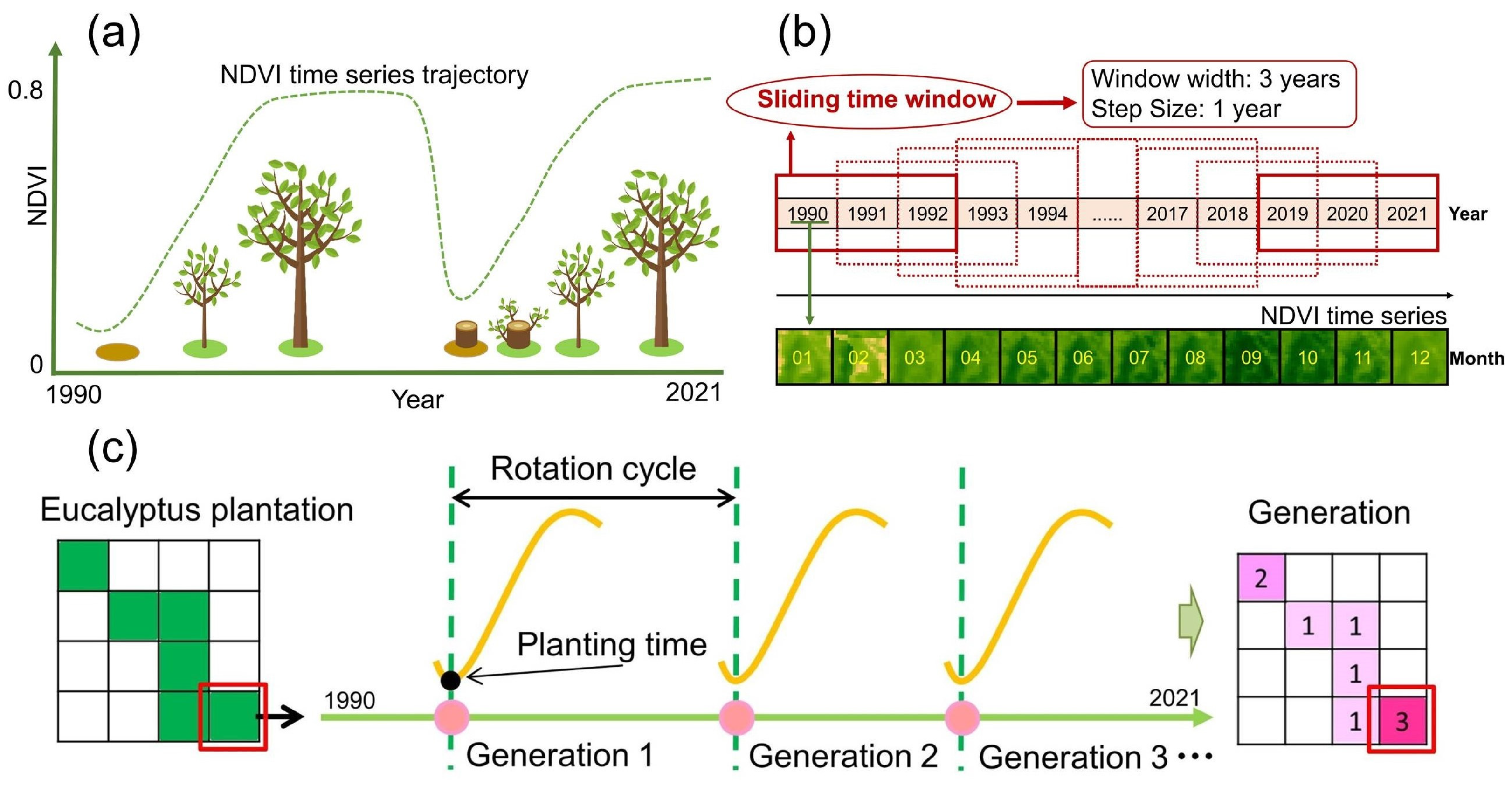
3.1. Time-Series Reconstruction

The NDVI [45] is the most widely used vegetation index and is sensitive to changes in vegetation ecosystem parameters. It uses the strong reflectance of vegetation in the NIR band and its significant difference from the red band to monitor the active photosynthetic biomass [46]. The NDVI represents the health of vegetation, with high values indicating healthy plants and low values indicating an absence or low quantity of vegetation. This vegetation index has been successfully applied in previous studies in similar contexts [19,47,48]. The NDVI was calculated as follows:
NDVI = ( N I R R e d ) ( N I R + R e d )
We used the NDVI to analyze the dynamics of the eucalyptus plantations. Using only annual time-series methods may potentially lead to the misclassification of rapidly growing eucalyptus plantations as forests, as well as other plantations due to harvesting, or even as farmland if the regrowth of eucalyptus NDVI in the first year matches the NDVI increase in other agricultural fields [21]. Therefore, to accurately detect variations in eucalyptus plantation events, including planting and growth processes, a denser time series is essential. This approach will ensure the comprehensive capture of key dynamics, fulfilling the criteria for effective eucalyptus change detection analysis. We used all available Landsat images and calculated the monthly NDVI rather than the yearly time series as the LandTrendr input. We performed monthly maximum compositing of the NDVI time series to achieve a more uniform time series and enhance the signal-to-noise ratio.

3.2. Sliding-Time-Window Principle and Width Determination

For a given pixel, the objectives of this study were to identify eucalyptus plantation planting and cutting events within the NDVI time series, determine the planting dates, and determine the rotation generation of fast-growing eucalyptus plantations through cutting and regeneration events. The eucalyptus identification and detection method used was based on specific growth changes in eucalyptus plants that manifest within a certain segment of the NDVI time series. Fast-growing eucalyptus rotation plantations usually have an apparent rotation cycle encompassing planting, growing, cutting, and regeneration phases (Figure 5a). In the first rotation, seeding cultivation is adopted, and these seedlings are transplanted into the field and take 1–2 months to establish stable root systems, during which their NDVI values are relatively low. Once established, trees begin to flourish and rapidly increase their leaf area and the corresponding NDVI values. Over the subsequent three to four years, the eucalyptus plantations maintain dense vegetation cover and a high level of NDVI until the trees are harvested. After entering the next rotation cycle (Figure 5c), the second rotation typically employs coppice regeneration; the rotation cycle for fast-growing eucalyptus is generally 3–6 years, although it can extend from 3 to 8 years. The unique characteristics of rapid planting, stable growth, cutting, and regeneration within such a short period have led to unique changes in the growth cycles of eucalyptus plantations. Therefore, the objective of this study was to identify key changes in eucalyptus trees in the NDVI time series.
To capture the pivotal changes in eucalyptus plantations, we introduced a sliding time window (Figure 5b) to segment the NDVI time series, which could be used specifically for our study area with frequent cloud and rain cover in subtropical regions. We first divided the inter-year time-series data into several subsequences to increase the data quantity while reducing the computational complexity. The segmented subsequences reflect the information of the original data to the greatest extent possible [49,50]. Based on the biological characteristics and rotational patterns of eucalyptus plantations, we defined a sliding window width of three years (36 months) [21,22,30]. After determining the width of the sliding window, we used the monthly NDVI time-series data within each sliding window width to obtain eucalyptus growth information and used this sliding window width as the length of time for the LandTrendr algorithm. To ensure that the changes at the beginning and end of the window could be accurately detected, we used a moving step size of 1 year for the sliding time window. A time series with a time length m is represented as follows:
Y = (y(t1), y(t2), …, y(tm))
where y(ti) are data obtained at time ti and the acquisition time ti is strictly increased. Starting in January 1990 and ending in December 2021, the NDVI time series was segmented into 30 overlapping subsequences using the sliding-time-window approach.

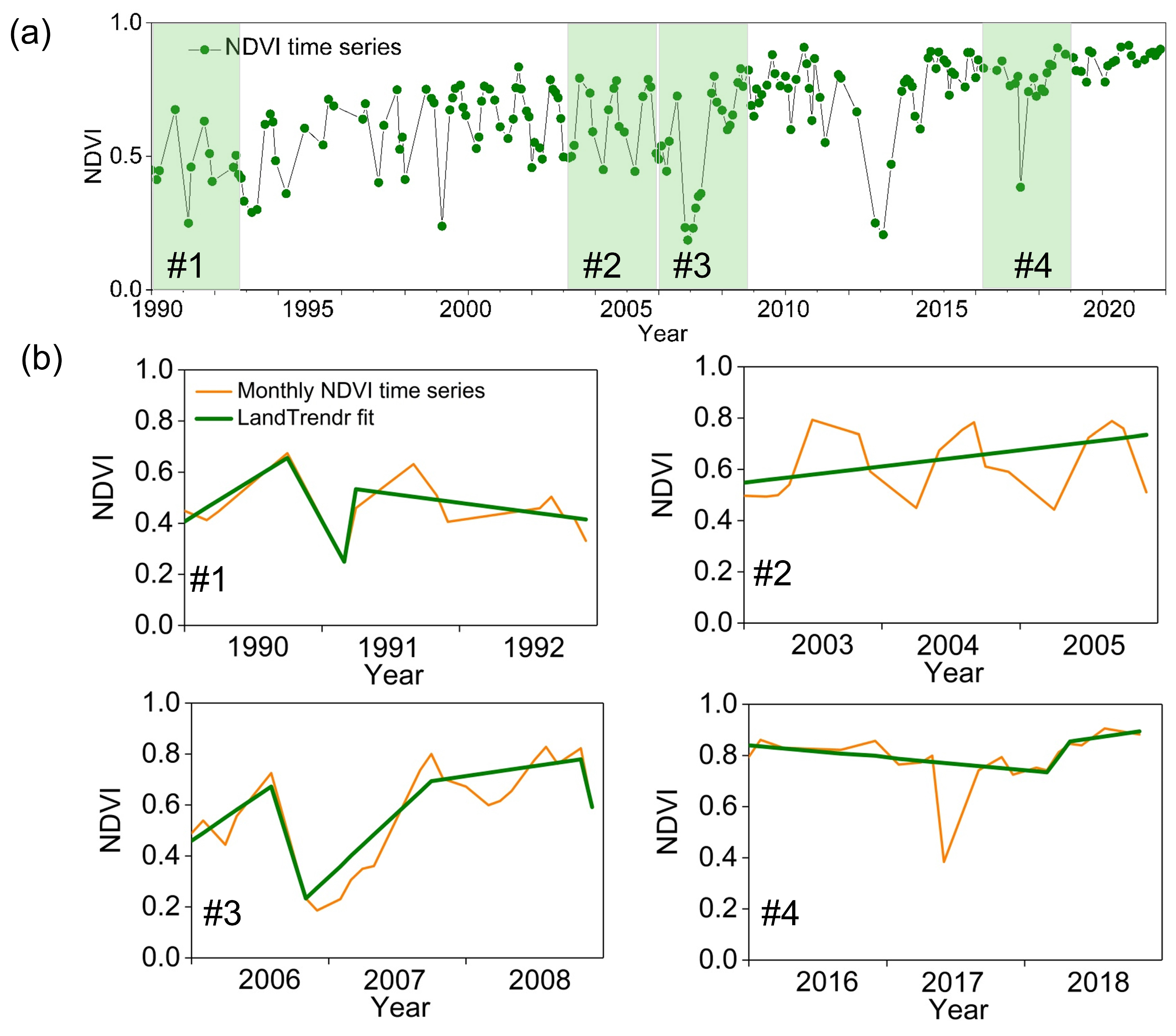
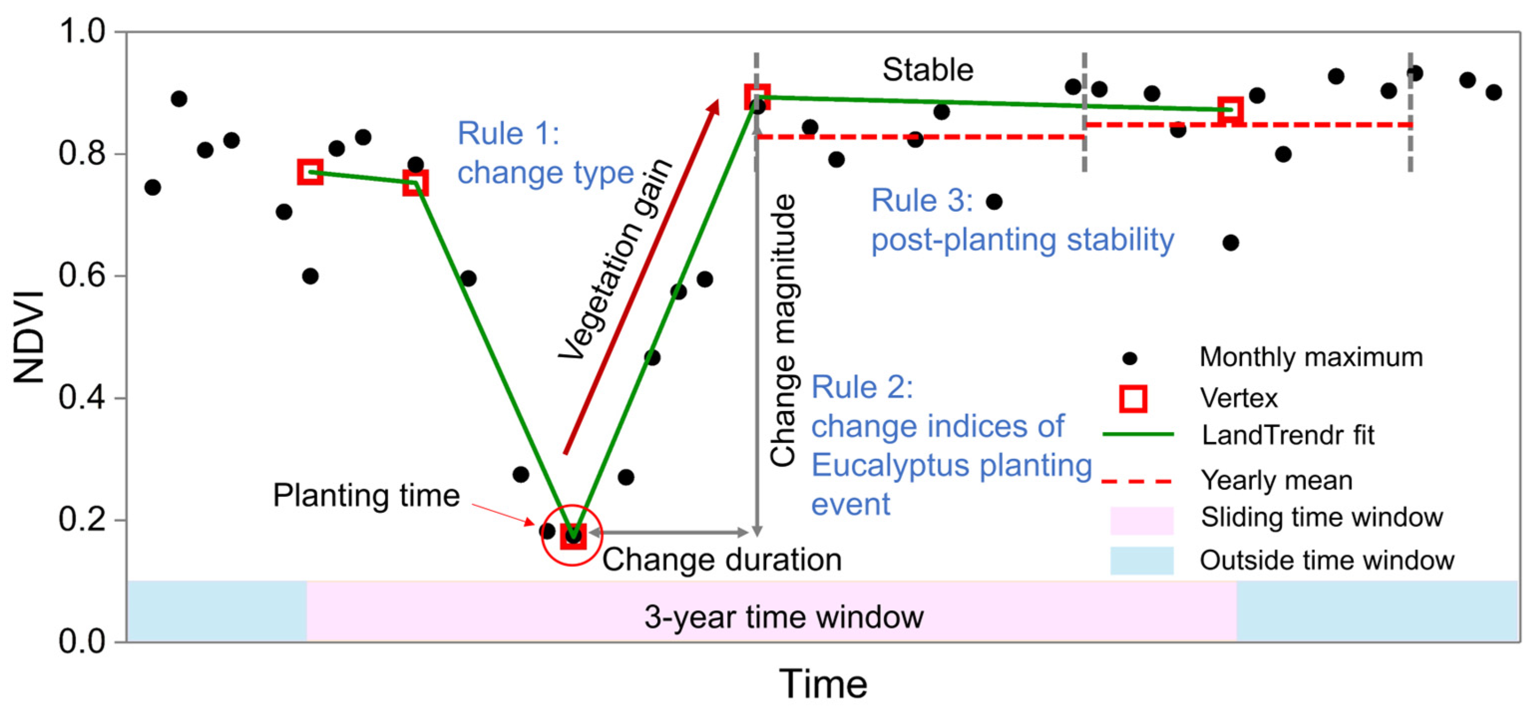
3.3. LandTrendr Detection with Sliding Time Window

The LandTrendr method is a widely applied algorithm based on the segmentation analysis of temporal trajectories and has been implemented for change detection analysis with the GEE [25]. This algorithm is composed of a series of spectral–temporal segmentation algorithms designed to identify disturbance events and changing trends at the pixel level from spectral trajectories, and can approximate the rate and timing of changes. The segmentation of spectral–temporal trajectories is achieved through a sequence of breakpoints and straight segments, which provides a simpler representation of the temporal–spectral trajectories and helps eliminate the noise present in the time series [23]. LandTrendr was originally developed for monitoring terrestrial forest disturbance and is suitable for detecting annual changes in vegetation cover induced by sudden events [51]. The temporal segmentation process, which is inherently complex in its algorithmic implementation, necessitates a series of tests to determine the optimal set of parameters for any given band/index and forest area. These operational parameters are crucial in guiding the algorithm to achieve an optimal fitted temporal trajectory representation of the disturbances. Furthermore, spectral filtering of the LandTrendr temporal segmentation results further constrains the captured spectral changes to specific disturbance types and sources. This aids in analyzing and capturing changes in the characteristics of eucalyptus plantations [52,53,54]. However, LandTrendr segmentation relies on a single observation or value for each year and determines the “best available pixels” for annual composites by selecting the start and end dates of the compositing period. Annual time-series data could potentially filter out the crucial growth or harvesting phases of fast-growing eucalyptus plantations, thus limiting a comprehensive capture of the dynamics of these plantations.
In this study, a sliding time window-based LandTrendr implemented in the GEE was applied to capture the temporal trajectory changes of eucalyptus plantations using an intra-year monthly time series within the sliding time window to detect the crucial growth or harvesting phases of fast-growing eucalyptus plantations. On a pixel-by-pixel basis, the sliding time window-based LandTrendr algorithm employs NDVI subsequence segments, acquired through sliding time windows, for trajectory fitting. The NDVI subsequences are then processed using LandTrendr’s temporal segmentation. The algorithm operates with fixed segmentation parameter values for any given band/index, facilitating this as a standard procedure (Figure 6), which preserves the original time-series trajectories to the maximum extent while amplifying the change information to some degree. Cutting and growth changes in eucalyptus plants have significant characteristics in the NDVI time series. Based on these temporal segments, various indicators can be derived, including the type of change (vegetation loss and growth), duration, magnitude, interval, and change occurrence time.
Compared to the original LandTrendr algorithm, adding a sliding time window to the LandTrendr algorithm handles more-complex spectral trajectories owing to the utilization of monthly NDVI time-series data. Thus, a careful configuration of the key parameters of the algorithm is required. First, the maximum segment parameters limit the number of trend segments allowed during the fitting process. Second, the de-spiking parameter limits the influence of single outliers with higher values, resulting in less smoothing and, consequently, less spike elimination. Third, the recovery threshold determines the maximum segment length, which represents a positive trend. All three parameters contribute to separating the change signals closer to the eucalyptus plantation from the captured variations. Finally, the sliding time window-based LandTrendr algorithm requires setting the p-of-F value, which determines the goodness of fit. In our pursuit to optimally capture the required change patterns through our enhanced algorithm, we experimented with various parameter values and selected the optimal operational parameters by visually assessing the trajectory fitting across different samples (Table 1) [23].

3.4. Eucalyptus Planting Dynamics Analysis

For each subsequence, by adding a sliding time window into the LandTrendr algorithm, we detected the presence of eucalyptus rotation events within the time series. By analyzing the patterns of eucalyptus changes, we developed change detection rules to determine the planting times of the eucalyptus (Figure 7). To determine the characteristics of growth changes during each stage of eucalyptus plantation growth, a typical trajectory of eucalyptus NDVI was determined, as shown in Figure 5a and Figure 8a. Before planting, land consolidation leads to lower NDVI values; the NDVI increases rapidly in the first two years after planting, reaches a high value, and then fluctuates seasonally until felling. Based on this unique and evident characteristic, we identified eucalyptus planting events by matching the NDVI change patterns. The sequence identified as eucalyptus was determined by analyzing the monthly NDVI data for the first three years following planting. Utilizing NDVI time-series data for each pixel from 1990 to 2021, with a three-year sliding window for iterative analysis, we documented the dynamics of eucalyptus plantations in Guangxi from 1990 to 2019.
A total of 250 pure eucalyptus pixels were selected from the images, ground-checked, and compiled. Several metrics were calculated for each subsequence in every sliding time window: magnitude, duration, rate, and mean NDVI value of the first and second years after planting. Statistical graph analysis revealed that the majority (˃95%) of eucalyptus plantation forests transitioned from initial planting to stable growth. In contrast, the average NDVI values for the two years after planting remained stable above 0.7 (Figure 8b) and exhibited magnitude values ranging from 0.25 to 0.86 (Figure 8c), which represents the duration of eucalyptus growth stages from 3 to 17 months and change rates between 200 and 20 (Figure 8d). In summary, we developed the pattern-matching rule described in Equations (3) and (4) to differentiate changes in the cultivation of eucalyptus plantations from other variations. The accurate identification of eucalyptus planting events enables a precise description of the eucalyptus plantation growth cycle and facilitates the determination of eucalyptus generations. Therefore, we sequentially evaluated each sequence and applied the aforementioned rules to perform pattern matching on the analyzed sequence to determine whether it corresponded to a eucalyptus planting event. In this study, the initial identification of eucalyptus planting events was designated as a first-generation forest, whereas subsequent identifications were classified as second-generation forests. The period from the onset of the first planting to the commencement of the second planting was regarded as the complete rotation cycle.
T C = Mag 0.25 3 D u r 17 20 R a t e 200
TNDVI = NDVI1st ≥ 0.7 & NDVI2nd ≥ 0.7
where TC is the threshold for change indicators and TNDVI is the threshold for NDVI values two years after the change. NDVI1st represents the average NDVI value one year after eucalyptus planting (regeneration), and NDVI2nd denotes the average NDVI value two years after eucalyptus planting (regeneration).

3.5. Accuracy Assessment

To validate the accuracy of the eucalyptus plantation and rotation maps, we followed good practices for accuracy assessment [55]. Validation points were derived from a random sample based on visual interpretation of Landsat time series and high-resolution imagery from Google Earth (if available), along with ground-truth sampling data. An accuracy assessment was conducted using regions of interest (ROIs) at both the pixel and plantation scales. Classification accuracy was evaluated by computing a confusion matrix comprising 494 eucalyptus plantation ROIs (13,001 pixels) and 255 non-eucalyptus plantation ROIs (15,612 pixels) and assessed through overall accuracy (OA), producer accuracy (PA), and user accuracy (UA). The accuracy of the planting times and eucalyptus generations was assessed using a dataset comprising 103 eucalyptus sample points representing diverse generations, encompassing 193 distinct planting events. Among the selected samples, 38 samples were from the first generation, 43 samples were from the second generation (86 planting years), 19 samples were from the third generation (57 planting years), and 3 samples were from the fourth generation (12 planting years), totaling 193 eucalyptus planting years. We directly compared our estimates with the actual planting years of the samples, which were evaluated using R2 and Root Mean Square Error (RMSE).

4. Results

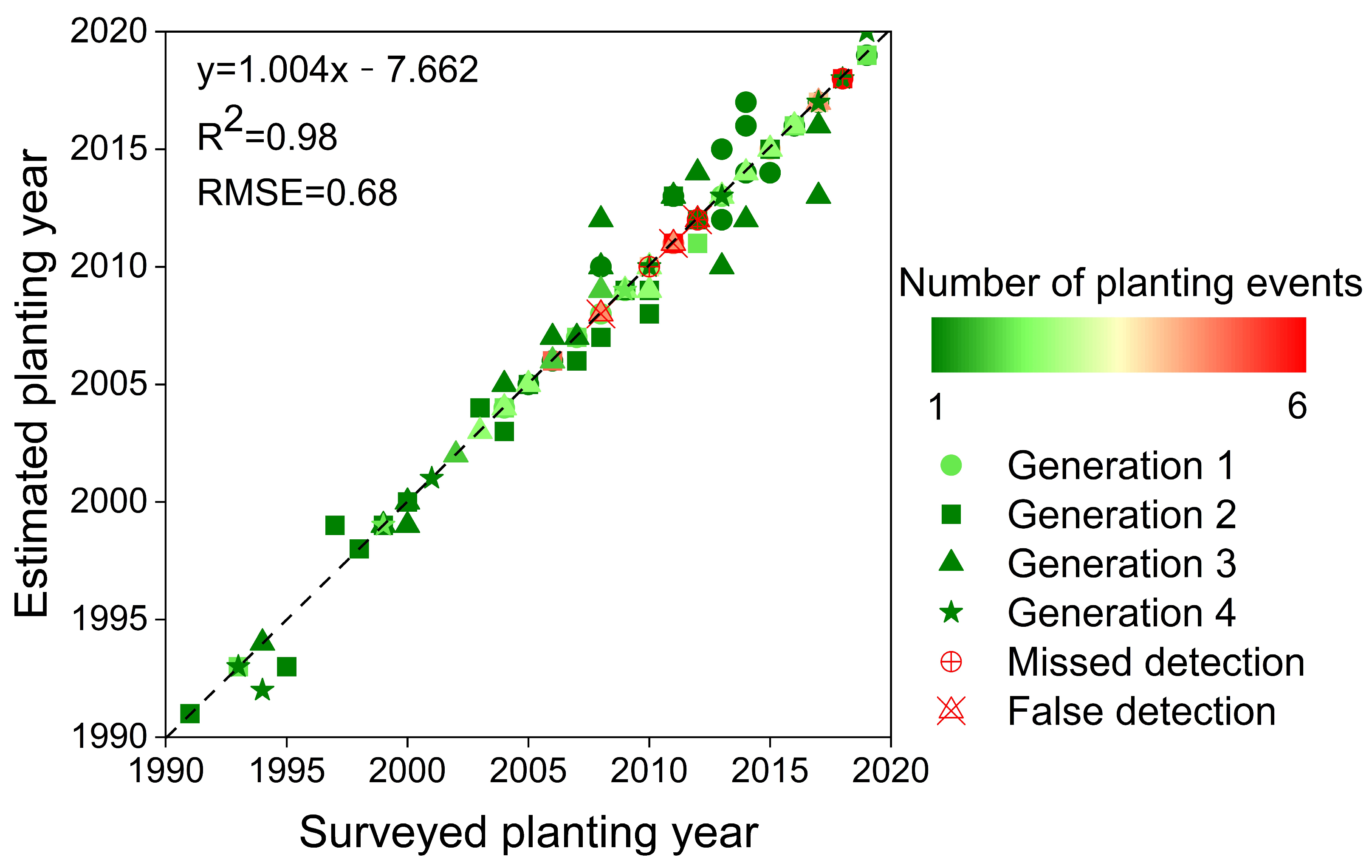
4.1. Accuracy Assessment of Eucalyptus Planting History

We implemented the detection method with time stacks of Landsat NDVI since 1990 and automatically generated historical planting years for the eucalyptus plantations in Guangxi from 1990 to 2019. The accuracy of the overall eucalyptus distribution was assessed using the validation samples described in Section 3.5. We evaluated the extraction of eucalyptus tree dynamics from two perspectives by overlaying the validation samples on the resultant map. First, we assessed the accuracy of the eucalyptus tree distribution using a confusion matrix (Table 2). The OA of the successive eucalyptus classification was 90.87%. The PA and UA for eucalyptus classification were 90.75 and 89.32, respectively. For eucalyptus plantations, the error described by the PA was larger than that described by the UA, indicating a slight overestimation with the proposed method. Various factors contributed to this phenomenon, but the primary factors were errors caused by cloudy and rainy weather conditions.
Furthermore, eucalyptus tree samples of different generations and ages were selected to evaluate the results. Figure 9 shows a scatter diagram of the planting years of the samples and the planting years estimated using our algorithm, which reveals a significant linear relationship. The overall RMSE of the two data sources was 0.68. Additionally, the regression line showed an apparent correlation (R2 = 0.98). Although the accuracy of the results was good, some false and missed detections existed: there were six instances of missed detection errors and two instances of false detection errors. The maximum difference between the estimated and surveyed samples in planting years was two years, which may be attributed to a significant deviation in the change-point localization caused by noise affecting the linear fitting process of the change detection algorithm.

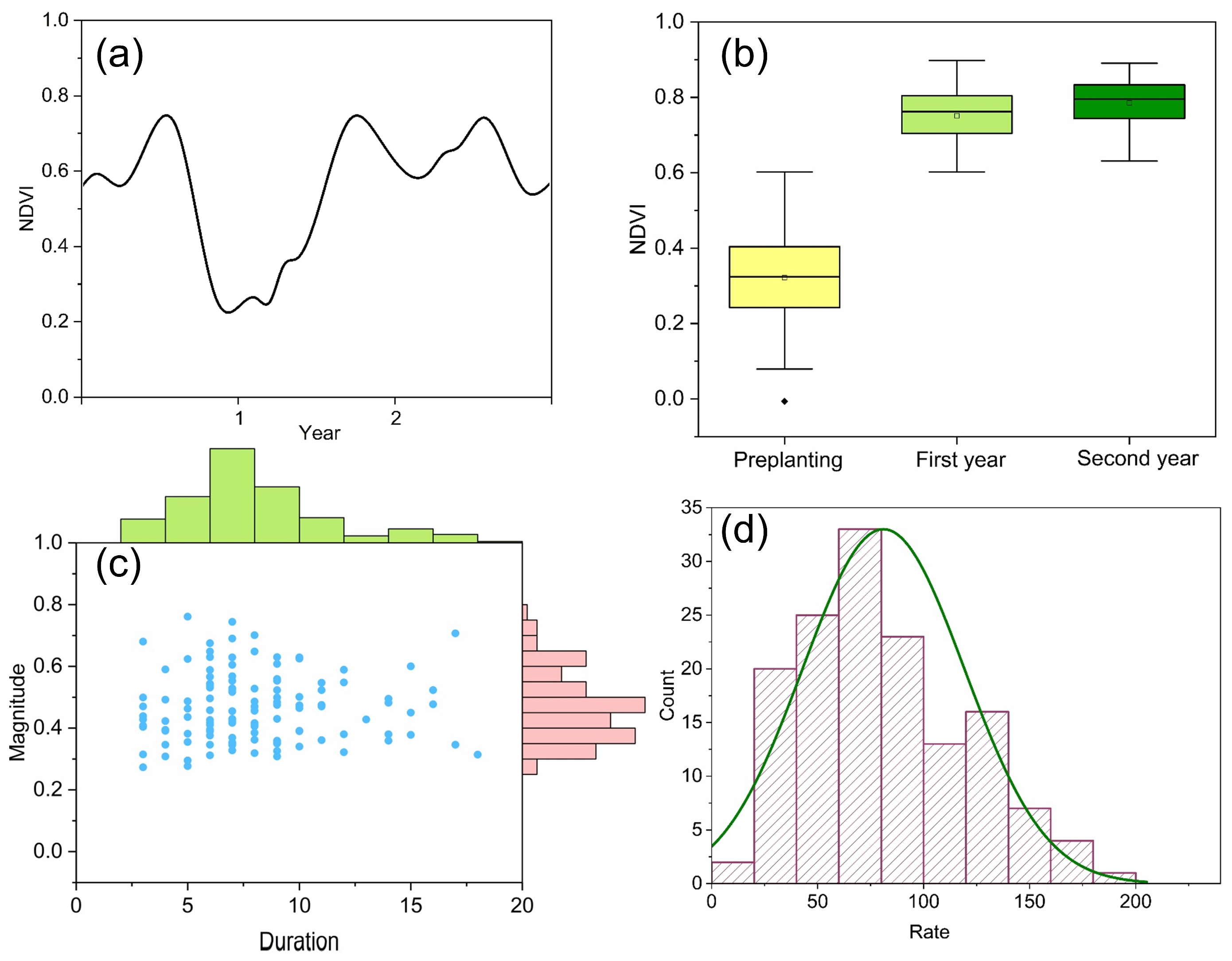
4.2. Detection of Eucalyptus Planting Events

Using a sliding time window, the entire NDVI time series was divided into 30 segments. Under the set of decision rules described in Section 3.3 and Section 3.4, the long-term dynamic time series of vegetation in eucalyptus plantations can accurately detect planting events. During the 30 years from 1990 to 2019, multiple eucalyptus planting events may have occurred. Retrieving monthly planting dates is impractical because of frequent cloud cover interference and the relatively low repetition rate of Landsat. Our final product determined the overall distribution of eucalyptus and documented the annual eucalyptus planting in Guangxi.
As an illustration, we selected two points within the Gaofeng Forest eucalyptus plantation, which have different planting times, to demonstrate the nuanced capability of our detection methodology (Figure 10a). Gaofeng Forest is a state-operated planted forest in Guangxi, where eucalyptus stands as the predominant tree species, and planting activities are frequent [56]. Figure 10b,c feature high-resolution historical Google Earth images from 2017 and 2019, respectively, vividly showcasing the state of the eucalyptus plantations. This visual evidence supports the algorithm’s effectiveness in capturing the detailed status of eucalyptus plantation development over time. The temporal variations in the NDVI reflect the rapid growth of eucalyptus plantations in the early stages of planting, reaching a stable state with high NDVI values within three years after planting (Figure 10d). The detection algorithm was employed to fit the segmented NDVI subsequences, dividing them into multiple linear segments, with the vertices between the segments serving as critical nodes for determining the planting dates. Figure 10 collectively demonstrates the successful identification of key eucalyptus planting events at the specified points, with the most recent events being in 2009 and 2018 for points P1 and P2, respectively.
An annual planting map of eucalyptus was produced for the years 1990–2019, covering the entire extent of Guangxi (Figure 11a,b). Eucalyptus plantations were mainly distributed in the central and southern parts of the study area. Large blocks of detected pixels represented plantations managed by state-owned forest enterprises, and small clusters represented patches held by local peasants and small companies.
The annual planting area was derived based on the yearly planting distribution map (1990–2019). A comparative analysis of the eucalyptus plantation area estimates between 2013 and 2018 indicated a close correspondence between our eucalyptus plantation data and the area figures reported by Deng et al. (Figure 11c) [4]. The area of eucalyptus plantations showed an increasing trend, peaking in 2011 and 2014. Further scrutiny of the Landsat data and high-resolution Google Earth images revealed that a significant amount of farmland was converted into eucalyptus plantations during these years.

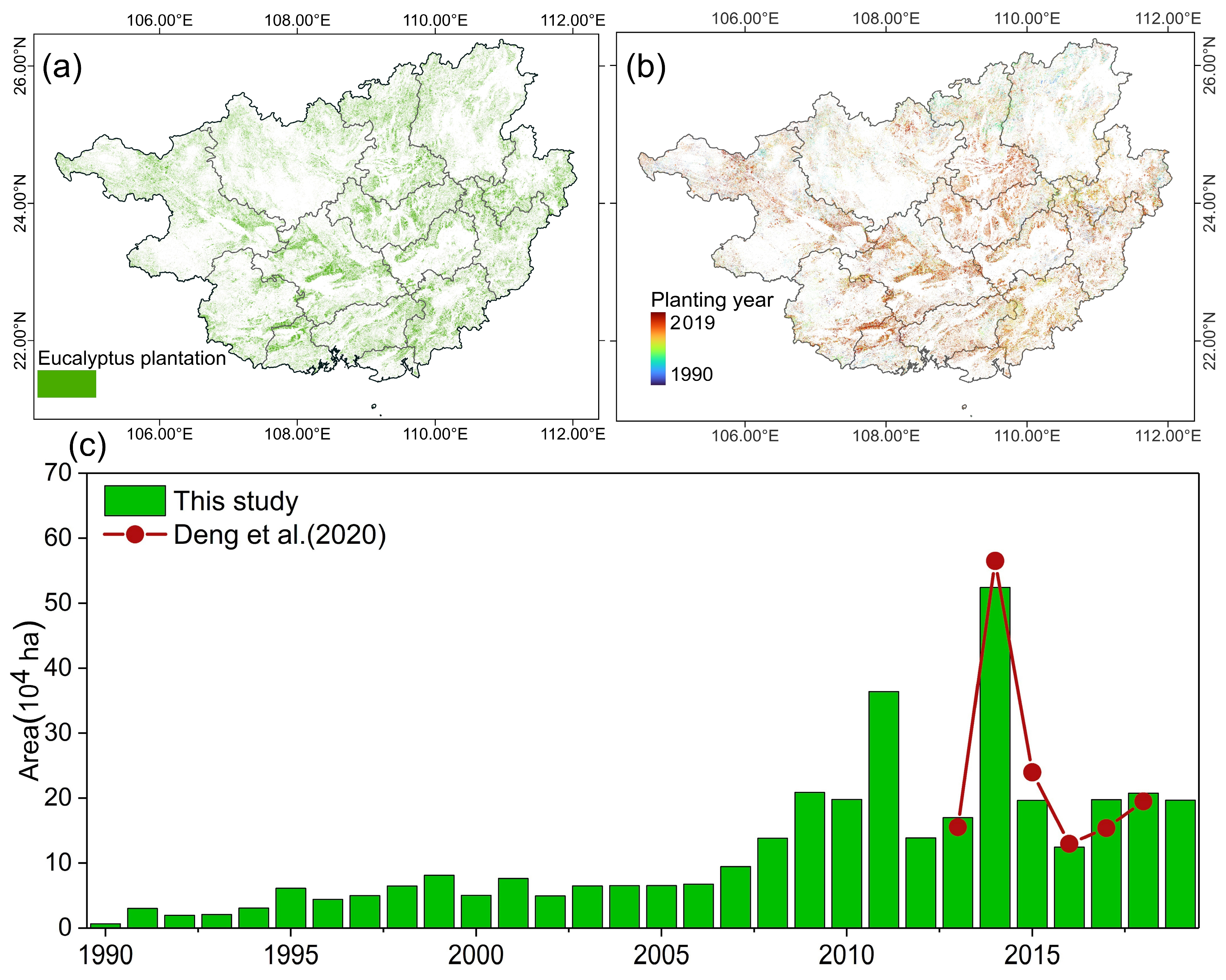
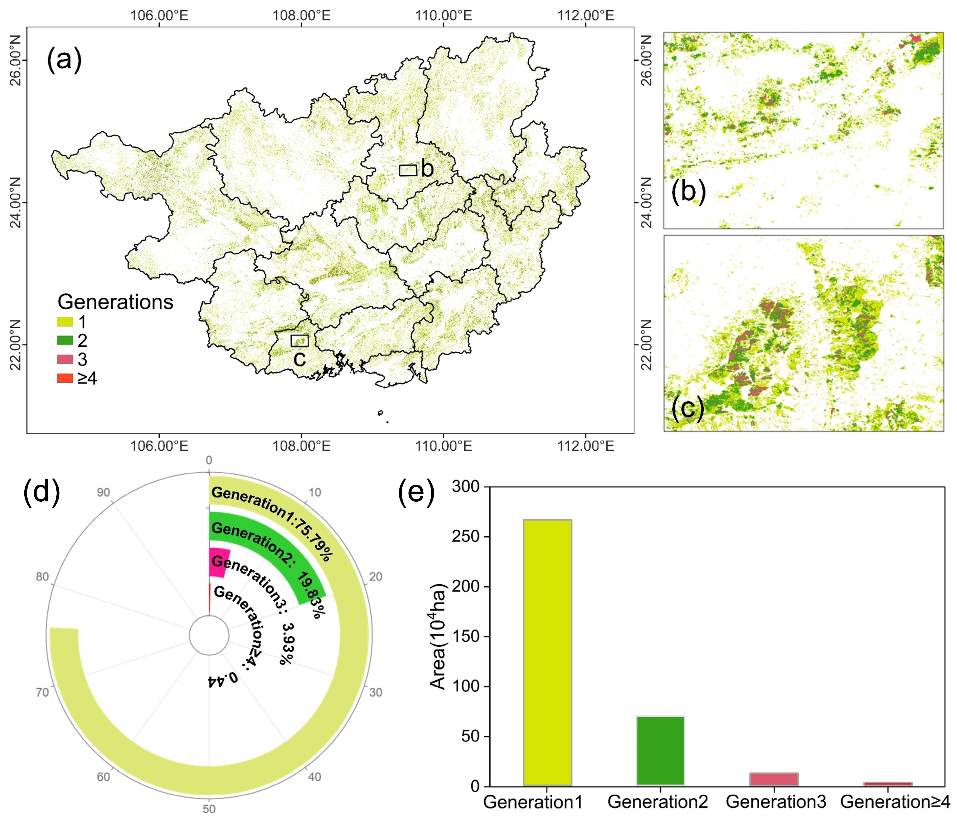
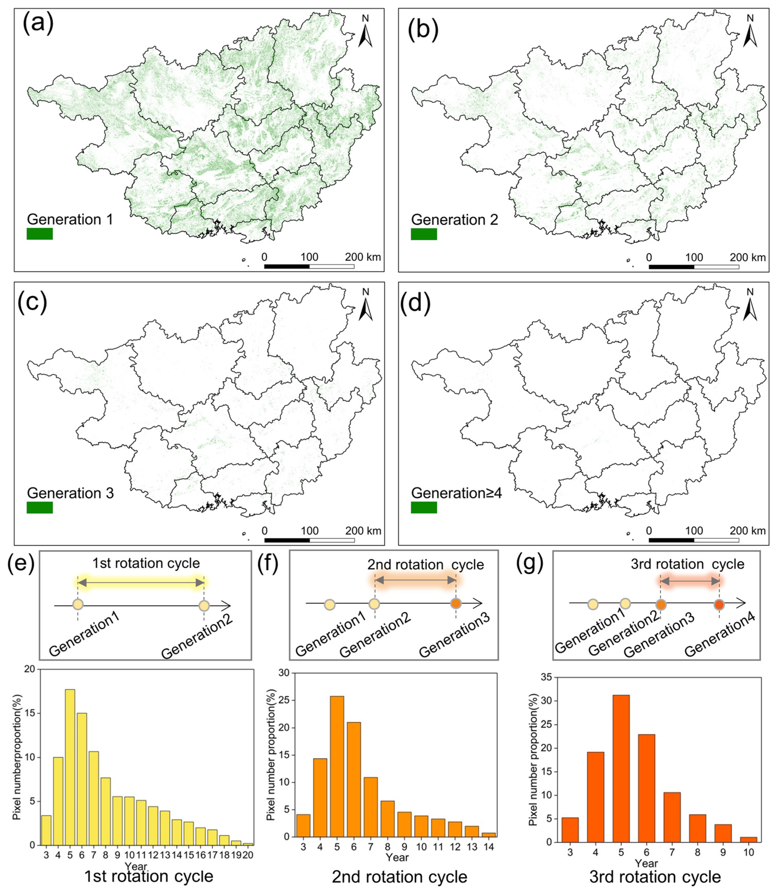
4.3. Spatial and Temporal Patterns of Eucalyptus Planting History Dynamics

We reconstructed the planting history of eucalyptus trees from 1990 to 2019 and identified all planting changes at the pixel level. Until 2019, eucalyptus plantations in Guangxi were mainly dominated by first- and second-generation forests, accounting for 95% of the entire rotation system (Figure 12a). The first-generation eucalyptus forests were mainly distributed in areas expanding outwards from the multi-generation eucalyptus forest regions (Figure 12b,c). The areas of first-generation, second-generation, third-generation, and greater-than-fourth-generation forests were 2,669,566, 698,564, 138,490, and 15,589 ha, respectively, representing 75.79%, 19.83%, 3.93%, and 0.44% of the total eucalyptus area (Figure 12d,e). This distribution pattern indicates a continuous expansion trend of eucalyptus plantations in recent years. Multi-generation rotations were mainly concentrated in the central region of the eucalyptus plantations.
Pixels with complete rotation cycles were selected for analysis. The predominant rotation cycles for eucalyptus trees ranged from 4 to 8 years. The average rotation cycle for the first rotation of eucalyptus was 8 years, the second rotation averaged 6.4 years, and the third rotation averaged 5.5 years (Figure 13). This suggests that, in the study area, the management of eucalyptus plantations was mainly characterized by short-term rotations. The spatial pattern of eucalyptus planting management was fragmented, with small patches being the primary focus of regeneration and distinct logging boundaries.

5. Discussion

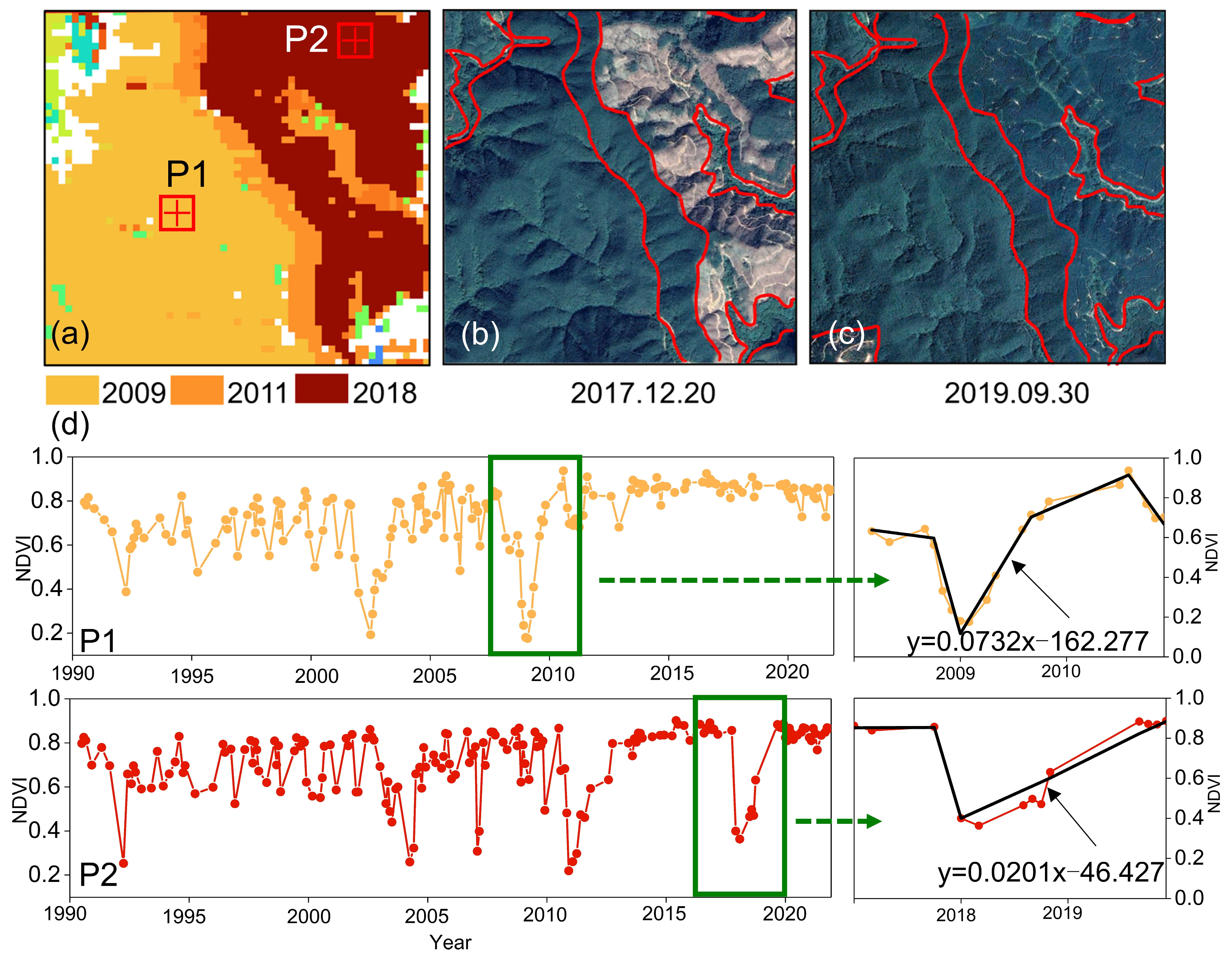
5.1. Advantages of the Sliding-Time-Window Series Change Detection Algorithm

This study innovatively proposed combining sliding-time-window segmentation with change detection analysis to obtain eucalyptus planting history information, utilizing dense Landsat time-series data and enhancing temporal information by segmenting the time series, which partially overcomes the challenges of capturing and discerning rapid changes using change detection algorithms. The application of a sliding time window allows the detection of rapid and subtle changes as well as facilitating multiple detections over time. This is particularly relevant for detecting changes in eucalyptus trees, considering their rapid growth rate and the practice of multiple rotational plantings. Sufficient observational data are required to support the algorithm, and global change detection algorithms tending to exhibit more false positives and misses when detecting eucalyptus changes. This is mainly due to the need for a certain interval length between breakpoints in global change detection algorithms to achieve model fitting.
To improve the LandTrendr algorithm, several researchers have transitioned from using single-band and single-spectral index inputs to incorporating multiple bands and spectral indices collectively to determine the final changes. Researchers have also considered data quality enhancements, integrated Sentinel data, and leveraged the availability of positive optical images to enhance the quality of time-series data and improve the accuracy of the algorithm. However, to the best of our knowledge, no study has improved the input of the LandTrendr algorithm to accommodate dense time-series data. For global change detection, excessive input data in LandTrendr can lead to overfitting of the regression algorithms, making it difficult to accurately identify change points. However, this study employed a sliding time window-based approach within the context of dense time-series data, thereby once again segmenting the sequences. This approach allows the capture of subtle changes without causing overfitting issues in the algorithm. This demonstrates its significant capacity for effectively capturing rapid changes.

5.2. Potential Use of Eucalyptus Planting History Information

Eucalyptus has the potential to provide greater biomass than alternative biomass vegetation in the same land area. Despite their significant economic importance, optimal rotation strategies are not always adopted in eucalyptus plantation management because of the lack of information on eucalyptus rotation. Moreover, the accurate identification of the spatiotemporal dynamics of eucalyptus logging, growth, and rotation plays a crucial role in providing carbon sequestration services to ecosystems. Over the years, numerous forest disturbance detection methods and studies on change factors have been developed for different artificial forest tree species, and significant research has focused on the dynamics of forest and afforestation recovery disturbances in temperate and tropical regions. However, studies on monitoring large-scale fast-rotation eucalyptus plantations are limited. In contrast, our study provides a comprehensive framework for obtaining the historical dynamics of eucalyptus planting, and the results showed that the rotation cycle of eucalyptus was mostly four to eight years, which is similar to the related literature. Some studies have identified rotational dynamics in cultivated lands, yet many of these analyses are based on annually synthesized time series. Although annually synthesized time-series data can enhance image quality, they often lose a substantial amount of surface change details and processes, failing to fully depict vegetation growth dynamics. In particular, their identification performance may be suboptimal for frequent and intense disturbances. Our method introduces a new perspective and a potential avenue for detecting short-term rapid disturbance changes and pattern-based detection. The validation of the planting time ultimately showed that the information obtained regarding eucalyptus logging and planting through the sliding-time-window and pattern-matching change detection had an acceptable level of accuracy.
For fast-growing plantations, different tree species exhibit unique growth cycles and change patterns, all characterized by the capability to rapidly develop through planting. By analyzing the growth characteristics of various tree species, appropriate sliding time windows can be set to capture the planting phase or key growth periods of plantations, thereby identifying plantations and obtaining their spatiotemporal dynamics. The approach presented in this paper offers valuable insights for the dynamic recognition of other fast-growing plantations and short-rotation vegetation. This methodology enhances our ability to monitor and manage these plantations more effectively, contributing to the optimization of their economic and ecological benefits. Through the application of this method, we can improve the accuracy of carbon stock estimates and support the sustainable management of fast-growing plantations. This ensures their ongoing role as resources for both carbon sequestration and biomass production.

5.3. Limitations and Potential Improvement

Although the proposed sliding time window-based change detection method showed excellent performance in our local study, there are limitations and areas for improvement. First, the combination of time-series segmentation using sliding time windows and subsequent change detection analysis proved effective in our study. However, forest changes are complex, as disturbances can arise from storm damage, forest fires, drought stress, pests, disease outbreaks, or logging activities. The extent of change and recovery rates significantly vary. More-sensitive change detection methods might more accurately identify such changes but could also introduce more false change points in stable forest ecosystems. In the process of analyzing the planting change patterns of eucalyptus using sliding time windows, we rely on NDVI values from two years post change to make determinations about these patterns. As a result, we are unable to capture the most recent two years of eucalyptus planting activities. Therefore, using Landsat data from 1990 to 2021, we can only detect eucalyptus plantation dynamics up to the year 2019. This time lag represents a significant limitation of our study, as it restricts our ability to provide up-to-the-minute insights into eucalyptus plantation status and changes. Future research could explore methods to reduce this lag and improve the timeliness of change detection in fast-growing plantations. Second, although we utilized all available Landsat imagery to compose the monthly time series, the frequent clouds and rain cover in Guangxi limited the quantity of high-quality optical observations in certain areas. As shown in Table 2, for eucalyptus plantations, the error described by the PA was 6.47% larger than that described by the UA, indicating a slight overestimation in the proposed method. Various factors contribute to this phenomenon, but the primary factor is errors caused by cloudy and rainy weather conditions, which could lead to a slight underestimation of the eucalyptus plantation area. In conclusion, although the STWCD method presented in this study shows promise, its application and performance should be further evaluated and improved in various contexts.

6. Conclusions

We have developed a novel change detection algorithm, STWCD, leveraging all available Landsat data and the GEE cloud-computing platform. This algorithm focuses on capturing key changes during the growth process of eucalyptus by constructing time windows, enabling the identification of eucalyptus pixels and the acquisition of the spatiotemporal dynamics of eucalyptus. Developed on an optimized LandTrendr framework, this workflow is highly sensitive to rapid vegetation changes, effectively pinpointing key transition moments in eucalyptus growth. We have uncovered the spatial distribution of eucalyptus rotation cycles over three decades in Guangxi, China, providing a clear depiction of the rotation periods for different eucalyptus generations. Our findings indicate a significant expansion in the area of eucalyptus plantations in Guangxi over recent decades, especially after 2011, with a peak in plantation area observed in 2014, aligning well with the implementation timeline of regional eucalyptus plantation management policies.
In summary, this method amplifies local information in NDVI time series through sliding-time-window segmentation and achieves precise temporal positioning of eucalyptus planting times by focusing on change characteristics. These results offer essential input data for assessing the quality of eucalyptus forests and modeling forest ecosystems. The biomass of plantations is a crucial carbon pool within forest ecosystems, and the obtained age information of eucalyptus also provides vital support for estimating carbon stocks.

Author Contributions

Conceptualization, Y.L. and X.L.; methodology, Y.L.; software, Y.L.; validation, Y.L., Z.H. and L.Z.; formal analysis, Y.L.; investigation, Y.L. and X.L.; resources, X.L.; data curation, Y.L. and L.Z.; writing—original draft preparation, Y.L.; writing—review and editing, M.L., L.W., Z.H., X.X. and L.T.; visualization, Y.L. and X.L.; supervision, X.L.; project administration, X.L.; and funding acquisition, X.L. All authors have read and agreed to the published version of the manuscript.

Funding

This research was funded by the National Natural Science Foundation of China under grant number 41871223.

Data Availability Statement

The data presented in this study are available on request from the corresponding author. The data are not publicly available due to privacy.

Conflicts of Interest

The authors declare no conflicts of interest.

References

  1. Wang, Y.; He, C.; Shi, Y.; Li, H.; Tang, Y.; Chen, B.; Ke, Q.; Wu, L.; Chen, L. Short-term cultivation limiting soil aggregate stability and macronutrient accumulation associated with glomalin-related soil protein in Eucalyptus urophylla x Eucalyptus grandis plantations. Sci. Total Environ. 2023, 878, 163187. [Google Scholar] [CrossRef] [PubMed]
  2. Chen, Y.; Peng, Z.; Ye, Y.; Jiang, X.; Lu, D.; Chen, E. Exploring a uniform procedure to map Eucalyptus plantations based on fused medium–high spatial resolution satellite images. Int. J. Appl. Earth Obs. Geoinf. 2021, 103, 102462. [Google Scholar] [CrossRef]
  3. Paine, T.D.; Steinbauer, M.J.; Lawson, S.A. Native and exotic pests of Eucalyptus: A worldwide perspective. Annu. Rev. Entomol. 2011, 56, 181–201. [Google Scholar] [CrossRef] [PubMed]
  4. Deng, X.; Guo, S.; Sun, L.; Chen, J. Identification of Short-Rotation Eucalyptus Plantation at Large Scale Using Multi-Satellite Imageries and Cloud Computing Platform. Remote Sens. 2020, 12, 2153. [Google Scholar] [CrossRef]
  5. Zhang, Y.; Wang, X. Geographical spatial distribution and productivity dynamic change of eucalyptus plantations in China. Sci. Rep. 2021, 11, 19764. [Google Scholar] [CrossRef]
  6. Wang, Z.; Wang, H.; Chen, Z.; Wu, Q.; Huang, K.; Ke, Q.; Zhu, L.; Lu, S.; Tang, Y.; Li, H.; et al. Ecological niche differences regulate the assembly of bacterial community in endophytic and rhizosphere of Eucalyptus. For. Ecol. Manag. 2022, 524, 120521. [Google Scholar] [CrossRef]
  7. Fan, G.; Lu, F.; Cai, H.; Xu, Z.; Wang, R.; Zeng, X.; Xu, F.; Chen, F. A New Method for Reconstructing Tree-Level Aboveground Carbon Stocks of Eucalyptus Based on TLS Point Clouds. Remote Sens. 2023, 15, 4782. [Google Scholar] [CrossRef]
  8. Du, H.; Zeng, F.; Peng, W.; Wang, K.; Zhang, H.; Liu, L.; Song, T. Carbon Storage in a Eucalyptus Plantation Chronosequence in Southern China. Forests 2015, 6, 1763–1778. [Google Scholar] [CrossRef]
  9. Zhang, C.; Li, X.; Chen, Y.; Zhao, J.; Wan, S.; Lin, Y.; Fu, S. Effects of Eucalyptus litter and roots on the establishment of native tree species in Eucalyptus plantations in South China. For. Ecol. Manag. 2016, 375, 76–83. [Google Scholar] [CrossRef]
  10. Brundu, G.; Pauchard, A.; Pyšek, P.; Pergl, J.; Bindewald, A.M.; Brunori, A.; Canavan, S.; Campagnaro, T.; Celesti-Grapow, L.; Dechoum, M.d.S.; et al. Global guidelines for the sustainable use of non-native trees to prevent tree invasions and mitigate their negative impacts. NeoBiota 2020, 61, 65–116. [Google Scholar] [CrossRef]
  11. Zhang, C.; Xiao, X.; Zhao, L.; Qin, Y.; Doughty, R.; Wang, X.; Dong, J.; Yang, X. Mapping Eucalyptus plantation in Guangxi, China by using knowledge-based algorithms and PALSAR-2, Sentinel-2, and Landsat images in 2020. Int. J. Appl. Earth Obs. Geoinf. 2023, 120, 103348. [Google Scholar] [CrossRef]
  12. Lan, X.; Du, H.; Peng, W.; Liu, Y.; Fang, Z.; Song, T. Functional diversity of the soil culturable microbial community in eucalyptus plantations of different ages in guangxi, South China. Forests 2019, 10, 1083. [Google Scholar] [CrossRef]
  13. Dos Reis, A.A.; Franklin, S.E.; de Mello, J.M.; Acerbi Junior, F.W. Volume estimation in a Eucalyptus plantation using multi-source remote sensing and digital terrain data: A case study in Minas Gerais State, Brazil. Int. J. Remote Sens. 2018, 40, 2683–2702. [Google Scholar] [CrossRef]
  14. Garcia-Gonzalo, J.; Borges, J.; Palma, J.; Zubizarreta-Gerendiain, A. A decision support system for management planning of Eucalyptus plantations facing climate change. Ann. For. Sci. 2014, 71, 187–199. [Google Scholar] [CrossRef]
  15. Zhou, X.; Zhu, H.; Wen, Y.; Goodale, U.M.; Zhu, Y.; Yu, S.; Li, C.; Li, X. Intensive management and declines in soil nutrients lead to serious exotic plant invasion in Eucalyptus plantations under successive short-rotation regimes. Land Degrad. Dev. 2020, 31, 297–310. [Google Scholar] [CrossRef]
  16. Xi, W.; Du, S.; Du, S.; Zhang, X.; Gu, H. Intra-annual land cover mapping and dynamics analysis with dense satellite image time series: A spatiotemporal cube based spatiotemporal contextual method. GIScience Remote Sens. 2021, 58, 1195–1218. [Google Scholar] [CrossRef]
  17. Wulder, M.A.; Loveland, T.R.; Roy, D.P.; Crawford, C.J.; Masek, J.G.; Woodcock, C.E.; Allen, R.G.; Anderson, M.C.; Belward, A.S.; Cohen, W.B. Current status of Landsat program, science, and applications. Remote Sens. Environ. 2019, 225, 127–147. [Google Scholar] [CrossRef]
  18. Nguyen, T.H.; Jones, S.D.; Soto-Berelov, M.; Haywood, A.; Hislop, S. A spatial and temporal analysis of forest dynamics using Landsat time-series. Remote Sens. Environ. 2018, 217, 461–475. [Google Scholar] [CrossRef]
  19. Duarte, L.; Teodoro, A.; Gonçalves, H. Deriving phenological metrics from NDVI through an open source tool developed in QGIS. In Proceedings of the Earth Resources and Environmental Remote Sensing/GIS Applications V, Amsterdam, The Netherlands, 23–25 September 2014; pp. 238–246. [Google Scholar]
  20. Zhang, S.; Cui, Y.; Zhou, Y.; Dong, J.; Li, W.; Liu, B.; Dong, J. A Mapping Approach for Eucalyptus Plantations Canopy and Single Tree Using High-Resolution Satellite Images in Liuzhou, China. IEEE Trans. Geosci. Remote Sens. 2023, 61, 1–13. [Google Scholar] [CrossRef]
  21. le Maire, G.; Dupuy, S.; Nouvellon, Y.; Loos, R.A.; Hakamada, R. Mapping short-rotation plantations at regional scale using MODIS time series: Case of eucalypt plantations in Brazil. Remote Sens. Environ. 2014, 152, 136–149. [Google Scholar] [CrossRef]
  22. Qiao, H.; Wu, M.; Shakir, M.; Wang, L.; Kang, J.; Niu, Z. Classification of Small-Scale Eucalyptus Plantations Based on NDVI Time Series Obtained from Multiple High-Resolution Datasets. Remote Sens. 2016, 8, 117. [Google Scholar] [CrossRef]
  23. Kennedy, R.E.; Yang, Z.; Cohen, W.B. Detecting trends in forest disturbance and recovery using yearly Landsat time series: 1. LandTrendr—Temporal segmentation algorithms. Remote Sens. Environ. 2010, 114, 2897–2910. [Google Scholar] [CrossRef]
  24. Cohen, W.B.; Yang, Z.; Kennedy, R. Detecting trends in forest disturbance and recovery using yearly Landsat time series: 2. TimeSync—Tools for calibration and validation. Remote Sens. Environ. 2010, 114, 2911–2924. [Google Scholar] [CrossRef]
  25. Kennedy, R.; Yang, Z.; Gorelick, N.; Braaten, J.; Cavalcante, L.; Cohen, W.; Healey, S. Implementation of the LandTrendr Algorithm on Google Earth Engine. Remote Sens. 2018, 10, 691. [Google Scholar] [CrossRef]
  26. Zhu, Z.; Woodcock, C.E. Continuous change detection and classification of land cover using all available Landsat data. Remote Sens. Environ. 2014, 144, 152–171. [Google Scholar] [CrossRef]
  27. Cai, Y.; Shi, Q.; Xu, X.; Liu, X. A novel approach towards continuous monitoring of forest change dynamics in fragmented landscapes using time series Landsat imagery. Int. J. Appl. Earth Obs. Geoinf. 2023, 118, 103226. [Google Scholar] [CrossRef]
  28. Verbesselt, J.; Hyndman, R.; Newnham, G.; Culvenor, D. Detecting trend and seasonal changes in satellite image time series. Remote Sens. Environ. 2010, 114, 106–115. [Google Scholar] [CrossRef]
  29. Wu, L.; Li, Z.; Liu, X.; Zhu, L.; Tang, Y.; Zhang, B.; Xu, B.; Liu, M.; Meng, Y.; Liu, B. Multi-Type Forest Change Detection Using BFAST and Monthly Landsat Time Series for Monitoring Spatiotemporal Dynamics of Forests in Subtropical Wetland. Remote Sens. 2020, 12, 341. [Google Scholar] [CrossRef]
  30. Li, D.; Lu, D.; Wu, Y.; Luo, K. Retrieval of eucalyptus planting history and stand age using random localization segmentation and continuous land-cover classification based on Landsat time-series data. GIScience Remote Sens. 2022, 59, 1426–1445. [Google Scholar] [CrossRef]
  31. Yan, J.; Wang, L.; Song, W.; Chen, Y.; Chen, X.; Deng, Z. A time-series classification approach based on change detection for rapid land cover mapping. ISPRS J. Photogramm. Remote Sens. 2019, 158, 249–262. [Google Scholar] [CrossRef]
  32. Pasquarella, V.J.; Arévalo, P.; Bratley, K.H.; Bullock, E.L.; Gorelick, N.; Yang, Z.; Kennedy, R.E. Demystifying LandTrendr and CCDC temporal segmentation. Int. J. Appl. Earth Obs. Geoinf. 2022, 110, 102806. [Google Scholar] [CrossRef]
  33. Tao, Z.; Xu, Q.; Liu, X.; Liu, J. An integrated approach implementing sliding window and DTW distance for time series forecasting tasks. Appl. Intell. 2023, 53, 20614–20625. [Google Scholar] [CrossRef]
  34. Ye, S.; Rogan, J.; Sangermano, F. Monitoring rubber plantation expansion using Landsat data time series and a Shapelet-based approach. ISPRS J. Photogramm. Remote Sens. 2018, 136, 134–143. [Google Scholar] [CrossRef]
  35. Runge, A.; Nitze, I.; Grosse, G. Remote sensing annual dynamics of rapid permafrost thaw disturbances with LandTrendr. Remote Sens. Environ. 2022, 268, 112752. [Google Scholar] [CrossRef]
  36. Forzieri, G.; Dutrieux, L.P.; Elia, A.; Eckhardt, B.; Caudullo, G.; Taboada, F.A.; Andriolo, A.; Balacenoiu, F.; Bastos, A.; Buzatu, A.; et al. The Database of European Forest Insect and Disease Disturbances: DEFID2. Glob. Chang. Biol. 2023, 29, 6040–6065. [Google Scholar] [CrossRef]
  37. Dara, A.; Baumann, M.; Kuemmerle, T.; Pflugmacher, D.; Rabe, A.; Griffiths, P.; Hölzel, N.; Kamp, J.; Freitag, M.; Hostert, P. Mapping the timing of cropland abandonment and recultivation in northern Kazakhstan using annual Landsat time series. Remote Sens. Environ. 2018, 213, 49–60. [Google Scholar] [CrossRef]
  38. Wang, J.; Xiao, X.; Liu, L.; Wu, X.; Qin, Y.; Steiner, J.L.; Dong, J. Mapping sugarcane plantation dynamics in Guangxi, China, by time series Sentinel-1, Sentinel-2 and Landsat images. Remote Sens. Environ. 2020, 247, 111951. [Google Scholar] [CrossRef]
  39. Zeng, W.; Tomppo, E.; Healey, S.P.; Gadow, K.V. The national forest inventory in China: History-Results-International context. For. Ecosyst. 2015, 2, 23. [Google Scholar] [CrossRef]
  40. Borchers, A.; Pieler, T. Programming pluripotent precursor cells derived from Xenopus embryos to generate specific tissues and organs. Genes 2010, 1, 413–426. [Google Scholar] [CrossRef] [PubMed]
  41. Gorelick, N.; Hancher, M.; Dixon, M.; Ilyushchenko, S.; Thau, D.; Moore, R. Google Earth Engine: Planetary-scale geospatial analysis for everyone. Remote Sens. Environ. 2017, 202, 18–27. [Google Scholar] [CrossRef]
  42. Xu, H.; Qi, S.; Li, X.; Gao, C.; Wei, Y.; Liu, C. Monitoring three-decade dynamics of citrus planting in Southeastern China using dense Landsat records. Int. J. Appl. Earth Obs. Geoinf. 2021, 103, 102518. [Google Scholar] [CrossRef]
  43. Roy, D.P.; Kovalskyy, V.; Zhang, H.K.; Vermote, E.F.; Yan, L.; Kumar, S.S.; Egorov, A. Characterization of Landsat-7 to Landsat-8 reflective wavelength and normalized difference vegetation index continuity. Remote Sens. Environ. 2016, 185, 57–70. [Google Scholar] [CrossRef] [PubMed]
  44. Foga, S.; Scaramuzza, P.L.; Guo, S.; Zhu, Z.; Dilley, R.D.; Beckmann, T.; Schmidt, G.L.; Dwyer, J.L.; Joseph Hughes, M.; Laue, B. Cloud detection algorithm comparison and validation for operational Landsat data products. Remote Sens. Environ. 2017, 194, 379–390. [Google Scholar] [CrossRef]
  45. Tucker, C.J. Red and photographic infrared linear combinations for monitoring vegetation. Remote Sens. Environ. 1979, 8, 127–150. [Google Scholar] [CrossRef]
  46. Schultz, M.; Clevers, J.G.P.W.; Carter, S.; Verbesselt, J.; Avitabile, V.; Quang, H.V.; Herold, M. Performance of vegetation indices from Landsat time series in deforestation monitoring. Int. J. Appl. Earth Obs. Geoinf. 2016, 52, 318–327. [Google Scholar] [CrossRef]
  47. Zhu, X.; Xiao, G.; Zhang, D.; Guo, L. Mapping abandoned farmland in China using time series MODIS NDVI. Sci. Total Environ. 2021, 755, 142651. [Google Scholar] [CrossRef]
  48. Bey, A.; Meyfroidt, P. Improved land monitoring to assess large-scale tree plantation expansion and trajectories in Northern Mozambique. Environ. Res. Commun. 2021, 3, 115009. [Google Scholar] [CrossRef]
  49. Li, R.; Xia, H.; Zhao, X.; Guo, Y. Mapping evergreen forests using new phenology index, time series Sentinel-1/2 and Google Earth Engine. Ecol. Indic. 2023, 149, 110157. [Google Scholar] [CrossRef]
  50. Panagiotakis, C.; Papoutsakis, K.; Argyros, A. A graph-based approach for detecting common actions in motion capture data and videos. Pattern Recognit. 2018, 79, 1–11. [Google Scholar] [CrossRef]
  51. Cohen, W.B.; Yang, Z.; Healey, S.P.; Kennedy, R.E.; Gorelick, N. A LandTrendr multispectral ensemble for forest disturbance detection. Remote Sens. Environ. 2018, 205, 131–140. [Google Scholar] [CrossRef]
  52. Yang, Y.; Erskine, P.D.; Lechner, A.M.; Mulligan, D.; Zhang, S.; Wang, Z. Detecting the dynamics of vegetation disturbance and recovery in surface mining area via Landsat imagery and LandTrendr algorithm. J. Clean. Prod. 2018, 178, 353–362. [Google Scholar] [CrossRef]
  53. de Jong, S.M.; Shen, Y.; de Vries, J.; Bijnaar, G.; van Maanen, B.; Augustinus, P.; Verweij, P. Mapping mangrove dynamics and colonization patterns at the Suriname coast using historic satellite data and the LandTrendr algorithm. Int. J. Appl. Earth Obs. Geoinf. 2021, 97, 102293. [Google Scholar] [CrossRef]
  54. Liu, Q.; Liu, L.; Zhang, Y.; Wang, Z.; Guo, R. Seasonal fluctuations of marsh wetlands in the headwaters of the Brahmaputra, Ganges, and Indus Rivers, Tibetan Plateau based on the adapted LandTrendr model. Ecol. Indic. 2023, 152, 110360. [Google Scholar] [CrossRef]
  55. Foody, G.M. Status of land cover classification accuracy assessment. Remote Sens. Environ. 2002, 80, 185–201. [Google Scholar] [CrossRef]
  56. Zhou, K.; Cao, L.; Liu, H.; Zhang, Z.; Wang, G.; Cao, F. Estimation of volume resources for planted forests using an advanced LiDAR and hyperspectral remote sensing. Resour. Conserv. Recycl. 2022, 185, 106485. [Google Scholar] [CrossRef]
Figure 1. Location of the study area (Guangxi, China) and the Landsat paths/rows used in this study.
Remotesensing 16 00744 g001
Figure 2. Landsat 5/7/8 Collection 1 Level-2 production used in this study. (a) Spatial distribution of total observation numbers and (b) clear observation numbers.
Remotesensing 16 00744 g002
Figure 3. Sample data based on high-resolution images and field sampling. (a) Spatial distribution of the samples and (b,c) photos of the eucalyptus.
Remotesensing 16 00744 g003
Figure 4. A flowchart of the overall approach.
Remotesensing 16 00744 g004
Figure 5. Constructing a sliding time window based on the growth characteristics of eucalyptus. (a) Diagram of the eucalyptus growth process, (b) sliding-time-window model in the time-series analysis, and (c) generation of eucalyptus within the sliding time window. The red box represents a schematic of pixel-wise detection.
Remotesensing 16 00744 g005
Figure 6. Example of the performance of the sliding time window-based LandTrendr algorithm in different windows: (a) shows the entire NDVI time series of a pixel from 1990 to 2021, with green semitransparent boxes representing four typical change detection windows, and (b) shows the algorithm’s treatment patterns for changes within these windows, including discarded changes, no significant mutations, output vegetation growth changes, and the algorithm’s handling of noise.
Remotesensing 16 00744 g006
Figure 7. The reference eucalyptus planting trajectory and relevant parameters used for matching were captured by LandTrendr-derived fitted trajectories of monthly NDVI time-series and sliding-time-window data.
Remotesensing 16 00744 g007
Figure 8. The key changing characteristic of eucalyptus: (a) NDVI time series corresponding to spectral changes in eucalyptus growth after planting, (b) NDVI of eucalyptus before and after planting, and (c,d) histograms of change detection indicators of eucalyptus reference samples.
Remotesensing 16 00744 g008
Figure 9. Comparison between the estimated and surveyed years of eucalyptus planting. The color code represents the number of eucalyptus trees planted in the same year.
Remotesensing 16 00744 g009
Figure 10. Identification of eucalyptus plantation events. (a) Examples of areas with different plantation events, (b,c) Google Earth images and the results of visual interpretation, and (d) the NDVI time series of sample points in the example area, and accompanied by the application of the STWCD algorithm to identify the last plantation event.
Remotesensing 16 00744 g010
Figure 11. Map of eucalyptus planting in Guangxi, China. (a) Overall distribution of eucalyptus trees, and (b) annual planting distribution of eucalyptus trees. (c) The temporal distribution of eucalyptus plantation areas; the green bars represent the annual eucalyptus planting areas identified in our study, and the red-dotted line graph represents the areas reported by Deng et al. (2020) [4].
Remotesensing 16 00744 g011
Figure 12. Map of eucalyptus plantation dynamics in Guangxi. (a) Spatial distribution of eucalyptus planting generations. (b,c) Two representative regions representing smallholder-based eucalyptus plantations and state-operated eucalyptus plantations. (d,e) Proportion and planting area of each generation.
Remotesensing 16 00744 g012
Figure 13. Distribution of eucalyptus plantations of different generations. (ad) Spatial distribution of the first-, second-, third-, and above-fourth generations of eucalyptus in Guangxi, China; (eg) illustrates the rotation cycle of different generations.
Remotesensing 16 00744 g013
Table 1. List of key parameters required for running the sliding time window-based LandTrendr algorithm in the Google Earth Engine (GEE), including the parameters, default values, and selected optimal values.
ParameterDefinitionDefaultValues
maxSegmentsMaximum number of segments to be fitted on the time series.68
spikeThresholdThreshold for dampening the spikes (1.0 means no dampening).0.90.9
vertexCountOvershootThe initial model can overshoot the maxSegments + 1 vertices by this amount. Later, it will be pruned down to maxSegments + 1.33
recoveryThresholdIf a segment has a recovery rate faster than 1/recoveryThreshold (in years), then the segment is disallowed.0.251.0
pvalThresholdIf the p-value of the fitted model exceeds this threshold, then the current model is discarded and another one is fitted using the Levenberg–Marquardt optimizer.0.10.15
bestModelProportionTakes the model with the most vertices that has a p-value that is at most this proportion away from the model with lowest p-value.1.250.75
minObservtionsNeededMinimum observations needed to perform output fitting.612
Table 2. Error matrix to calculate the OA, PA, and UA for the detection of eucalyptus identification.
ROIReferenceUA
%
EucalyptusNon-EucalyptusTotal
MapEucalyptus11,798141013,20889.32
Non-Eucalyptus120314,20215,40592.19
Total13,00115,61228,613
PA%90.7590.97 OA = 90.87
Disclaimer/Publisher’s Note: The statements, opinions and data contained in all publications are solely those of the individual author(s) and contributor(s) and not of MDPI and/or the editor(s). MDPI and/or the editor(s) disclaim responsibility for any injury to people or property resulting from any ideas, methods, instructions or products referred to in the content.

