
Enhancing Maize Yield Simulations in Regional China Using Machine Learning and Multi-Data Resources


1
School of Geographical Sciences, Nanjing University of Information Science & Technology, Nanjing 210044, China
2
Department of Infrastructure Engineering, The University of Melbourne, Parkville, VIC 3052, Australia
*
Author to whom correspondence should be addressed.
Remote Sens. 2024, 16(4), 701; https://doi.org/10.3390/rs16040701
Submission received: 5 January 2024
/
Revised: 27 January 2024
/
Accepted: 12 February 2024
/
Published: 16 February 2024
(This article belongs to the Topic Climate Change Impacts and Adaptation: Interdisciplinary Perspectives)
Abstract
:Improved agricultural production systems, together with increased grain yield, are essential to feed the growing global population in the 21st century. Global gridded crop models (GGCMs) have been extensively used to assess crop production and yield simulation on a large geographical scale. However, GGCMs are less effective when they are used on a finer scale, significantly limiting the precision in capturing the yearly maize yield. To address this issue, we propose a relatively more advanced approach that downsizes GGCMs by combining machine learning and crop modeling to enhance the accuracy of maize yield simulations on a regional scale. In this study, we combined the random forest algorithm with multiple data sources, trained the algorithm on low-resolution maize yield simulations from GGCMs, and applied it to a finer spatial resolution on a regional scale in China. We evaluated the performance of the eight GGCMs by utilizing a total of 1046 county-level maize yield data available over a 30-year period (1980–2010). Our findings reveal that the downscaled models created for maize yield simulations exhibited a remarkable level of accuracy (R2 ≥ 0.9, MAE < 0.5 t/ha, RMSE < 0.75 t/ha). The original GGCMs performed poorly in simulating county-level maize yields in China, and the improved GGCMs in our study captured an additional 17% variability in the county-level maize yields in China. Additionally, by optimizing nitrogen management strategies, we identified an average maize yield gap at the county level in China ranging from 0.47 to 1.82 t/ha, with the south maize region exhibiting the highest yield gap. Our study demonstrates the high effectiveness of machine learning methods for the spatial downscaling of crop models, significantly improving GGCMs’ performance in county-level maize yield simulations.
1. Introduction
By the year 2050, the global population is projected to exceed 9 billion, which is an increase of 2 billion people compared to the baseline year of 2010 [1]. As the population continues to expand, global food demand is also rapidly growing. The 25% increase in the global food demand by 2010 is projected to increase to 70% by 2050 [2,3] under ongoing climate warming and population growth, presenting serious food security challenges worldwide [4,5]. The Intergovernmental Panel on Climate Change (IPCC) Special Report on Climate Change and Land (SRCCL) highlights the fact that climate warming will trigger a series of cascading effects that will adversely affect food security [6]. A reduction in food production and the quality of grain will, in turn, pose threats to the development of agriculture-related industries and may exacerbate food shortages worldwide [7]. Given these concerns, achieving the “Zero Hunger” goal of the United Nations Sustainable Development Goals has become a top priority of national governments and other international communities [8]. In such a context, increasing crop production and accurately estimating crop yields by advancing appropriate models and technology are becoming increasingly crucial for global and regional food security [9,10].
Global gridded crop models (GGCMs) are some of the most significant tools being used extensively for estimating crop yields under various environmental and management conditions worldwide [11,12]. GGCMs have the ability to assess the impact of climate change on crop yields more effectively [13,14,15]. Researchers have parameterized crop growth processes using GGCMs by, for example, combining information such as weather, soil, and management parameters, followed by simulating the dynamics of crop growth and yield on regional and global scales [16,17]. Through analysis of the crop yield simulations of GGCMs, it has been revealed that climate change has been found to be the major driver causing a negative impact on global agricultural production [18]. A recent study by Yin and Leng [19] suggests that GGCMs effectively captured the adverse effects of climate change on maize production when using the 30-year (1980–2010) time series data on global climate change and maize production. Furthermore, GGCMs have been found to show varying performance in simulating major grain crop production in China [20]. GGCMs commonly use a 50 km × 50 km spatial resolution, which is suitable for robust crop yield assessments on a national scale [13]. However, there has been a rising concern that GGCM estimates at lower spatial resolutions may ignore real geographical factors, such as soil and topography [21]. One of the major concerns raised by researchers is that missing regional-level heterogeneity may lead to discrepancies between sub-grid level information and data and farm land and agricultural practices, consequently biasing the simulation model [22]. Conducting county-level maize yield studies poses challenges due to the lower resolution of GGCMs, making it challenging to identify spatial variations in maize yield [23]. Additionally, the utilization of global-scale datasets in the model results in considerable errors when simulating county-level maize yield, thereby hindering the effectiveness of local government efforts in risk prevention and decision making for food security [24]. Improved simulation accuracy of GGCMs at the county level holds the potential to significantly enhance research on crop yield loss risks spanning from local to regional scales; studies on potential crop yields will benefit significantly from such improvements [25,26]. On the other hand, applying gridded crop models at very high resolutions significantly increases computational demands and is often constrained by data availability [21]. GGCM crop simulations are primarily determined by climate data, but the global-scale higher-resolution climatic data needed have only been available at coarser spatial resolutions until recently [27].
An approach that can help address these issues efficiently and flexibly is downscaling the GGCM results, which has become significant in addressing unresolved issues of regional and global crop yield simulations and allows for obtaining high-resolution simulations without setting up high-resolution crop model infrastructures and comprehensive datasets [21]. Studies suggest that a machine learning-based downscaling approach could utilize correlations between dependent and independent predictor variables to refine low-resolution crop yield data into finer spatial-resolution data [28]. For instance, combining the GPM model and random forest increased the prediction potential of land productivity by accurately showing the reduction in the spatial-scale crop yield data from the United States [29]. Recently, machine learning and remote sensing variables have been employed to downscale global gridded crop yield data in southern Asia, which produced highly accurate results in crop yield at a 1 km resolution [30]. This suggests that when constrained by technical limitations and data accessibility, using machine learning to downscale low-resolution data into high-resolution data has become a viable approach for predicting crop production at both the regional and global scales [21]. However, currently, within agricultural sciences, this application has primarily been limited to the processing and analysis of remote sensing data [31,32]. Limited research on downscaling crop simulation yields from GGCMs has hindered generating unbiased results on global and regional crop yield simulations [21,33].
China is the world’s second-largest maize producer, contributing to 23% of global production in recent years [34]. Conducting research with a focus on ensuring maize yield in China is significant for global food security. We utilized the random forest algorithm and integrated climate data, soil data, and topographical data to downscale low-resolution data into high-resolution data to achieve the best possible model outcome. While downscaling the data, we used eight different GGCMs (e.g., CLM-CROP, GEPIC, EPIC-BOKU, EPIC-TAMU, EPIC-IIASA, PDSSAT, PAPSIM, PEGASUS) and calculated the ensemble mean of multiple GGCMs (ENSEMBLE). This enabled us to compare the model outputs, which assist in making better decisions. Taking China’s maize plantation regions as the research area, the primary objectives of this research were: (1) to develop precise downscaling models for simulating maize yields in regional China; (2) to evaluate the effectiveness of GGCMs in simulating maize yield, both before and after downscaling; (3) to compare and estimate maize yield disparities at the county level in China.
2. Methods and Datasets
2.1. Study Area
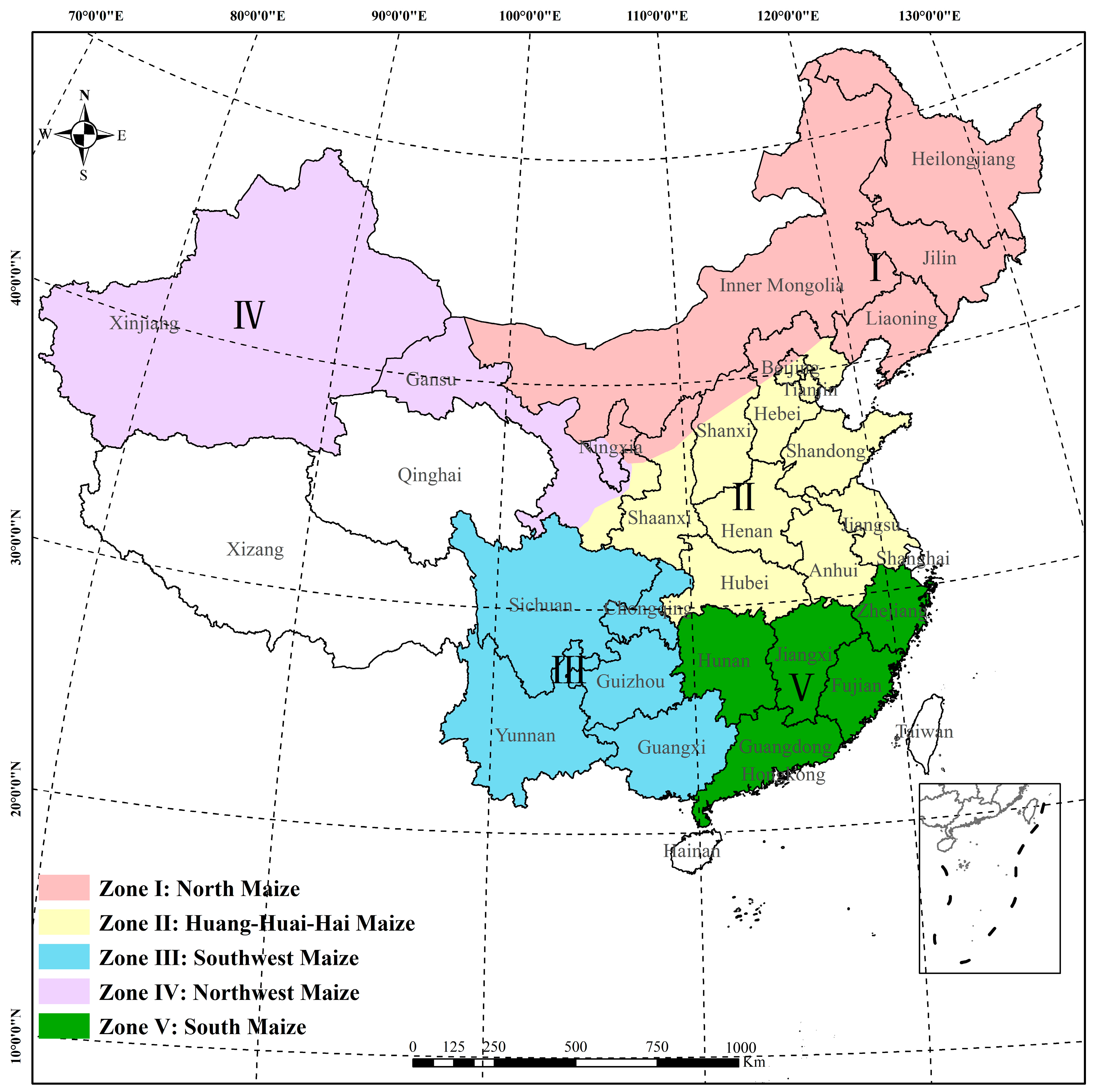
China’s maize plantation regions are classified into five distinct zones based on their cultivation characteristics, management practices, and geographical environments [35]. As shown in Figure 1, these zones contain the north spring maize region (Zone I), the Huang-Huai-Hai summer maize region (Zone II), the southwest maize region (Zone III), the northwest maize region (Zone IV), and the south maize region (Zone V). The mean annual temperature across these regions falls within approximately 9–25 °C, which is within the optimal range for maize growth, spanning from 9 to 29 °C [36]. Maize cultivation requires adequate water supply throughout its lifecycle [37]. Therefore, Zone IV accounts for only 3% of China’s annual maize cultivation area due to the low precipitation levels, while the remaining regions, with relatively higher precipitations, together account for 93% of the nation’s maize cultivation area.
2.2. Data Sources
2.2.1. Climate Data
In the Global Gridded Crop Model Intercomparison Project (GGCMI), all participating GGCMs adhered to a standardized protocol and were constrained by the same climate dataset [16,38]. We especially focused on one of the enforced simulations, namely the AgMERRA dataset, and thus, the gridded climate data were obtained from the publicly available AgMERRA climate dataset [27]. It features a spatial resolution of 25 km × 25 km and spans the period from 1980 to 2010. AgMERRA incorporates a comprehensive retrospective analysis of modern research and practical applications [39]. This dataset has been bias-corrected using station data and remote sensing data for agricultural land use. The selected key variables include the maximum temperature (TMAX), minimum temperature (TMIN), average temperature (TAVG), total precipitation (PRATE), potential evapotranspiration (PET), downward surface shortwave radiation (SRAD), wind speed (WS), and vapor pressure deficit (VPD) (Table 1). Several statistics were calculated for each climate variable, resulting in a total of 76 features.
2.2.2. Soil Data
Soil information was extracted from the Harmonized World Soil Database v1.2, featuring a spatial resolution of 1 km [40]. The dominant soil type was selected for each grid cell at a spatial resolution of 50 km from the largest soil mapping unit. We chose a total of 11 variables from the soil dataset, including the soil reference depth (DEPTH), bulk density in topsoil (BD), carbonate content in topsoil (CARB), cation exchange capacity in topsoil (CEC), clay content in topsoil (CLAY), electrical conductivity in topsoil (EC), organic carbon content in topsoil (OC), pH in topsoil (PH), coarse fragment (rock) content in topsoil (ROK), sum of bases in topsoil (SB), and soil sand content (SAND) (Table 1).
2.2.3. Topography Data
Topographical information was provided by digital elevation models (DEMs). DEMs are digital mapping datasets that consist of three-dimensional coordinates, typically derived from contour lines or photogrammetric methods [41]. We utilized a 1 km-resolution DEM sourced from the Space Shuttle Radar Topography Mission (SRTM) data. This dataset was derived from the latest SRTM V4.1 data (http://www.resdc.cn, accessed on 15 August 2023).
2.2.4. Irrigation Mask Data
To accurately evaluate the performance of each GGCM in simulating maize yields under both rain-fed conditions and irrigated conditions, we employed the mask data (irrigated and rain-fed crop harvested areas), to process the maize yield simulation results. The 1 km-resolution mask data were obtained from MIRCA2000 (https://www.uni-frankfurt.de/45218031/data_download, accessed on 15 August 2023), providing detailed information on the crop-specific irrigated and rain-fed harvested areas for each grid cell [42].
2.2.5. Maize Yield Data
To assess the performance of GGCMs, we used China’s county-level maize yield data. They were sourced from the Agricultural Statistical Yearbook compiled by the Ministry of Agriculture of China (http://www.stats.gov.cn, accessed on 15 August 2023), and its unit is kilograms per hectare (kg/ha). These data represent the average crop yield for each county and include both the rain-fed and irrigated maize yields.
2.2.6. Date Processing
Since maize yield data was available at the county-level, we aggregated the simulation results to the county scale using an area-weighted average, as described below:
where is the number of grid cells within each county, is the index of grid cell. represents the irrigated maize harvested area (ha) in grid cell , and is the rain-fed maize harvested area (ha) in grid cell . represents the simulated yield (t·ha−1) of irrigated maize in grid cell , and represents the simulated yield (t·ha−1) of rain-fed maize in grid cell .
Since variations in maize yields are mainly driven by management factors [43,44], and due to the limitations of accessible data, these influences should be removed from the maize yield data for an accurate evaluation of the GGCMs’ simulations. We employed a moving window approach spanning 5 years to eliminate trends in both the observed and simulated maize yields. This involved detrending the annual maize yield data by subtracting the yield mean in a 5-year window. Compared to other methods, this detrending approach has demonstrated greater effectiveness in mitigating the impact of trend effects [45].
2.3. Experiments Design
The primary objective of this research was to assess the feasibility of achieving high-resolution predictions using low-resolution simulated maize yield data. We employed a downscaling model constructed by the random forest algorithm. All the data were resampled to a uniform 50 km resolution, consistent with the spatial resolution of the maize yields simulated by GGCMs. Climate data, soil data, and topographical data were used as feature variables for model development, while the simulated maize yields served as the target variable. The data from 1980 to 2009 were randomly split into training and test sets, containing 75% and 25% of the samples, respectively. Data for the year 2010 were kept separate for data validation. Random forest exhibits greater flexibility in fitting training data, but it is also more prone to overfitting. To avoid overfitting, we employed various techniques, including monitoring out-of-bag error, performing n-fold cross-validation, and applying regularization to make the training procedure more conservative. We evaluated the high-resolution GGCM maize yield simulations after downscaling using observed county-level maize yield data from 1980–2010. As an example, we estimated the maize yield disparities for the year 2010.
2.3.1. Description for the Gridded Crop Model
The GGCMI (Global Gridded Crop Model Intercomparison Project) Phase 1 dataset comprises outputs from fourteen modeling groups, spanning various time periods and four major staple crops: soybeans, wheat, maize, and rice [16]. The GGCMI defined three distinct model configurations based on different crop management practices [44]. Firstly, each modeling group developed a “default” configuration (default) based on their typical historical period simulation management, technical assumptions, and inputs. Next, they developed a “full harmonization” configuration (Fullharm), which involved harmonized growing seasons (i.e., prescribed grid-cell- and crop-specific sowing and maturity dates) and fertilizer inputs. Lastly, simulations were conducted with the same harmonized growing seasons but with unlimited nutrient supply, termed the “Harmnon” configuration (Harmnon). All simulations were conducted under both rain-fed (noirr) and fully irrigated (irr) conditions to facilitate a closer approximation of crop yields to actual production in subsequent processing [46,47]. Due to the unavailability of simulation results for all model configurations from some groups, we utilized the data from only eight models (e.g., CLM-CROP, EPIC-BOKU, EPIC-IIASA, EPIC-TAMU, GEPIC, PAPSIM, PDSSAT, and PEGASUS). These GGCMs were driven by historical weather datasets, such as WFDEI, AgMERRA, WATCH (WFD), GRASP, AgCFSR, and Princeton GF (Table S1). Given that these weather datasets are all based on station data or reanalysis data, we assumed that the choice of different weather datasets had minimal impact on the simulation results.
2.3.2. Random Forest
The random forest (RF) algorithm stands as a well-established ensemble learning algorithm that performs regression or classification tasks by combining a large number of decision trees [48]. RF is particularly suitable for capturing both linear and nonlinear relationships between crop yields and various environmental factors [49,50]. RF offers a valuable feature by providing a metric for assessing the relative importance of different predictor variables. This capability aids researchers in better understanding how climate and soil variables influence maize yield, contributing to a more comprehensive understanding of the underlying factors driving crop production [51]. Numerous studies have demonstrated the good performance of RF in predicting county-level maize yields [52,53]. RF exhibits robustness to variations in data distribution and demonstrates less sensitivity to hyperparameter tuning [54]. Its ensemble learning approach helps mitigate overfitting concerns [54]. Additionally, RF’s default settings commonly yield satisfactory results, making it a practical choice. The model’s effectiveness may also stem from its ability to capture specific patterns or relationships in maize yield data and from its generally strong performance in diverse applications [55,56]. Since RF is less prone to overfitting, we struck a balance between its computational performance and efficiency by adjusting the global parameters, as its computational demands increase linearly with the number and depth of trees. The key parameters that required tuning for RF were as follows: the number of trees (n_estimators), the tree depth (max_depth), and the minimum number of samples required to split a node (min_samples_split). To optimize the downscaling model, we selected the parameters that minimized the RMSE through ten-fold cross-validation.
2.3.3. Feature Engineering and Feature Importance
Our features were derived from the model’s input data, as described in Section 2.2; they were climate, soil, and topographical data. Depending on the variable type, the daily climate data were averaged to the monthly average climate data, with the number following the variable name representing the month. Since maize in China is typically planted in April and harvested in October, we defined April to September as the growing season for the simulations [57,58]. The daily climate data were aggregated into seasonal averages and seasonal totals based on the maize growing season timeline. Soil data mainly consist of surface soil variables (0–30 cm, divided according to the HWSD), as surface soil mainly affects maize growth [21]. Additionally, relevant features affecting maize yield include DEM data, which serve as site-specific characteristics. This process is referred to as feature engineering, which involves normalizing raw data based on domain knowledge. RF can internally determine feature importance by initially splitting on a fixed feature, calculating the total reduction in the sum of squared residuals achieved by each tree as a result of this split, and averaging it over all trees, where larger averages indicate greater variable importance [51]. Here, we present the relative importance of each feature as a percentage and rank all features accordingly.
2.3.4. Calculation of Regional Maize Yield Gap
In the GGCMI, the input data for GGCMs in the Fullharm scenario were the same as that in the Harmnon scenario, except for the nitrogen fertilizer input data. In the Harmnon scenario, characterized by an unlimited nutrient supply, the simulated maize yield is referred to as the potential yield. This potential yield serves as the baseline for defining the yield gap and related analyses [16]. To quantify the difference in the simulated maize yields between the Harmnon and the Fullharm scenarios (t/ha), we calculated the maize yield gap by computing the multi-model ensemble mean using Equation (2):
where is the relative maize yield gap as the multi-model ensemble mean, is the number of GGCMs, is the member of GGCMs, is the simulated maize yield in the Harmnon scenario, and is the simulated maize yield in the Fullharm scenario.
2.4. Metrics for Model Performance Evaluations
The coefficient of determination (R²), the root-mean-square error (RMSE), and the mean absolute error (MAE) were applied to assess the effectiveness of the downscaling model developed in this study. Furthermore, we utilized the correlation coefficient (R), RMSE, and MAE to evaluate the performance of GGCMs in simulating the spatiotemporal variability of maize yield both before and after downscaling. The calculations for these metrics are provided in Equations (3)–(6):
where ( = 1, 2, …, ) is the number of samples, is the simulated maize yield, is the predicted maize yield, is the observed maize yield, and is the corresponding mean value.
3. Results
3.1. Performance of Simulated Maize Yield Downscaling Model
3.1.1. General Performance of Downscaling Model and Spatial Patterns of Maize Yield
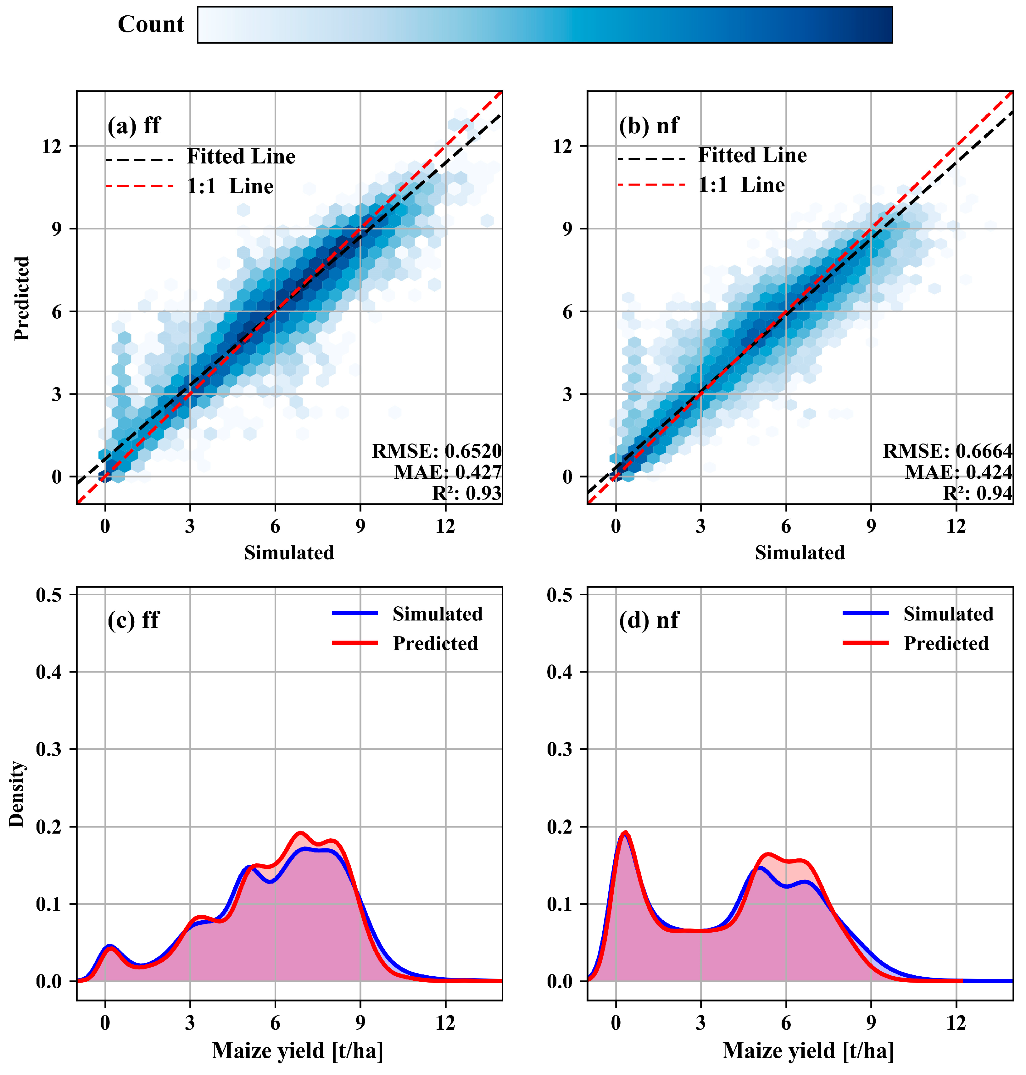
All GGCMs except PAPSIM showed exceptionally high goodness-of-fit and demonstrated low errors under both the irrigated and rain-fed conditions (R2 ≥ 0.9, RMSE < 0.75 t/ha, MAE < 0.5 t/ha) (Figures S1–S7). Notably, EPIC-BOKU exhibited the highest goodness-of-fit, with R2 = 0.93, RMSE = 0.65 t/ha, and MAE = 0.42 t/ha under irrigated conditions, and R2 = 0.94, RMSE = 0.66 t/ha, and MAE = 0.42 t/ha under rain-fed conditions (Figure 2a,b). Predominantly, maize yield overestimations occurred when the simulated yields were low, while underestimations were observed when the simulated yields were high (Figure 2c,d). Despite some deviations, the overall density distribution of the predicted yields closely resembles that of the simulated yields (Figure 2c,d). These deviations vary within different model-specific maize yield intervals. For all models, the range of simulated maize yields corresponding to the peak density in irrigated maize consistently surpassed that of the simulated rain-fed maize (Figures S1–S7). This indicates a significant improvement in maize yield following adequate irrigation. Due to the significantly low accuracy exhibited by PAPSIM’s downscaling model, it has been omitted from this study for further consideration.
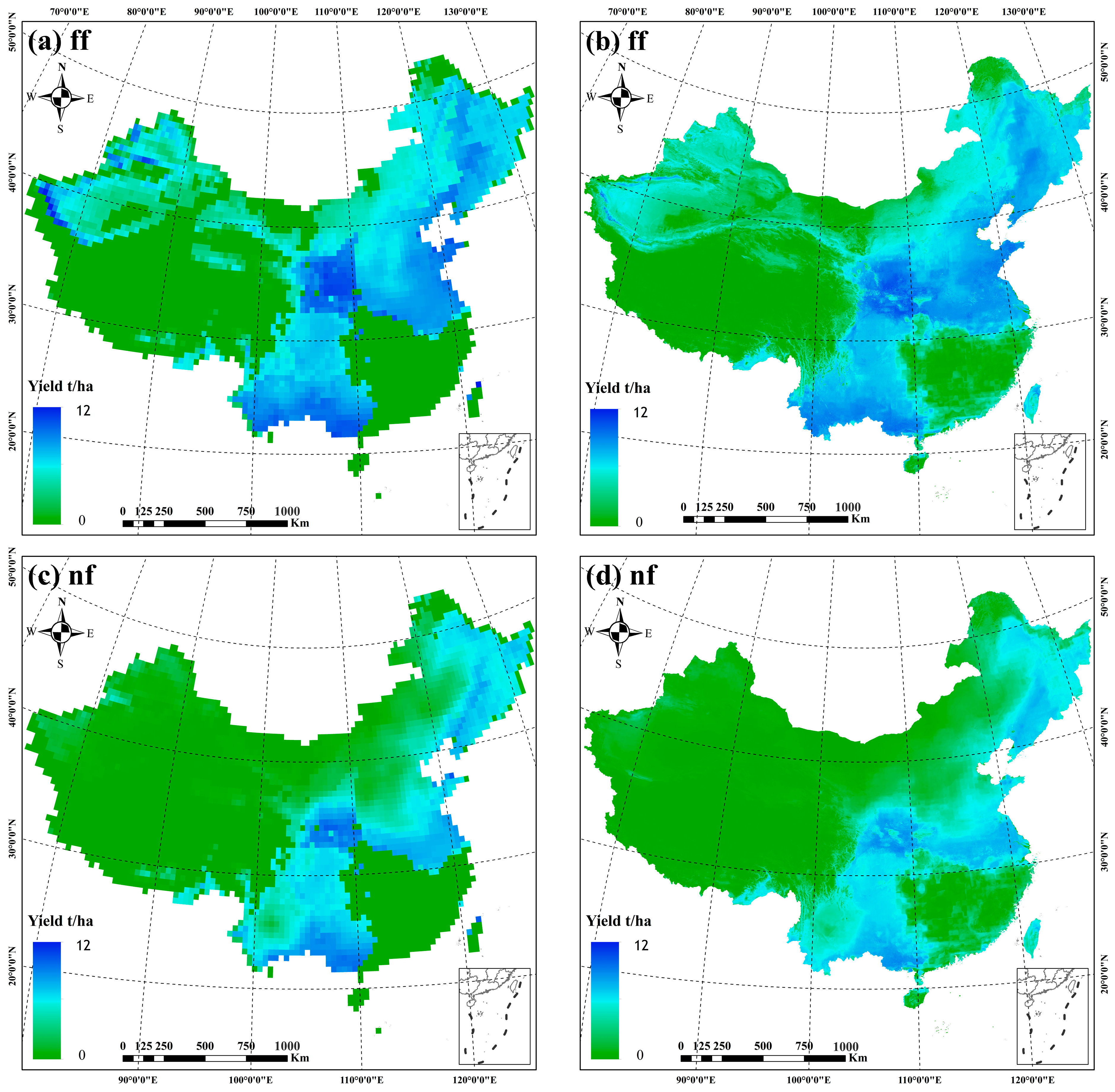
We compared the low-resolution simulations with the high-resolution machine learning predictions for maize yield in China in 2010 (Figures S8–S13). And here, taking EPIC-BOKU as an example (Figure 3), it was evident that for both the rain-fed and irrigated conditions, there was a consistent spatial distribution pattern observed in both the low-resolution simulations and the high-resolution machine learning predictions. The maize yields exhibited significant spatial heterogeneity under both the irrigated and rain-fed conditions, with the maize yield under the irrigated conditions being significantly higher than that under the rain-fed conditions (Figure 3 and Figures S8–S13). However, the high-resolution machine learning predictions outperformed the low-resolution simulations in accurately capturing the heterogeneity of the maize yield across China (Figure 3 and Figures S8–S13). This suggests that high-resolution machine learning predictions are more suitable for county-level maize yield studies in China compared to low-resolution simulations.
3.1.2. Feature Importance from Maize Yield Simulations
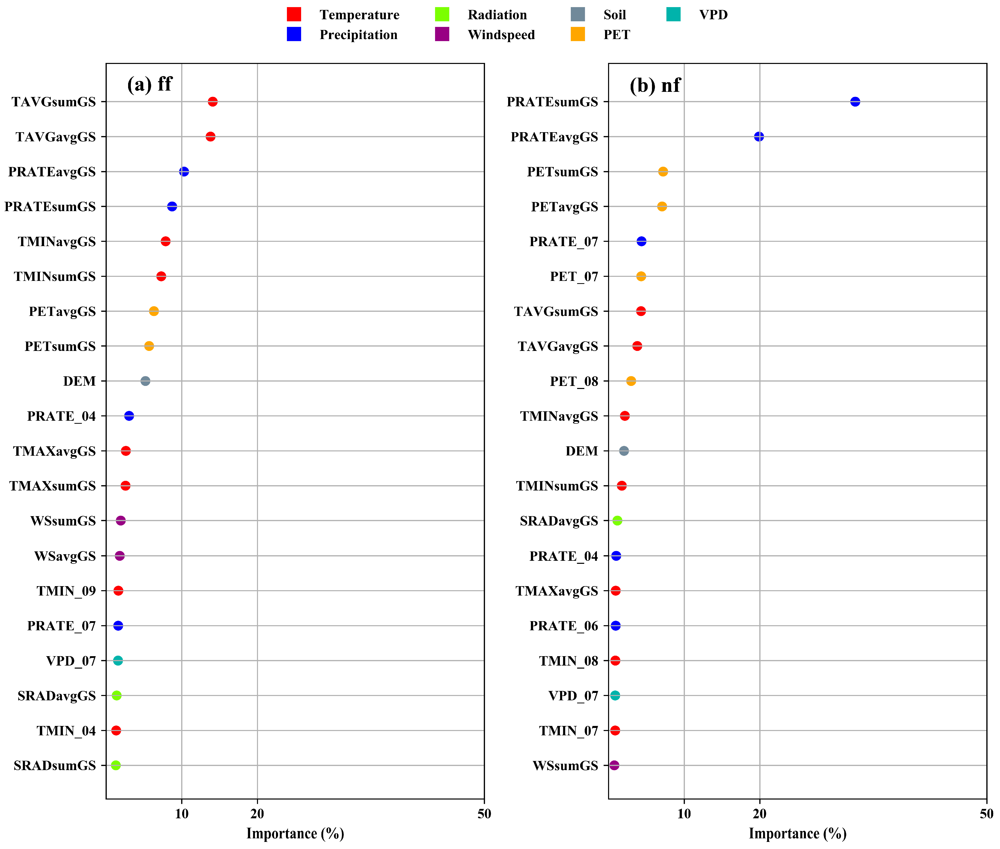
We calculated the feature importance for all models (Figures S14–S19), taking EPIC-BOKU as an example (Figure 4). In the rain-fed conditions, the most critical indicators for predicting maize yield consistently revolved around precipitation-related features. Following closely were features related to PET, temperature, and soil–terrain characteristics (Figure 4b and Figures S14b–S19b). Under adequate irrigation conditions, temperature-related features and VPD were the predominant indicators for maize yield, whereas the significance of precipitation-related features diminished (Figure 4a and Figures S14a–S19a). Whether the maize was rain-fed or irrigated, the climate characteristics during the maize growing season (e.g., PRATEsumGS, PRATEavgGS, TMINsumGS, TMAXsumGS, TMINavgGS, TMAXavgGS, TAVGsumGS, and TAVGavgGS) consistently ranked as pivotal indicators. This emphasizes that drought or excessive moisture during the growing season significantly impacts maize yield. Features related to soil and terrain characteristics played a relatively lesser role in maize yield predictions. DEM was the most relevant feature among the soil and terrain characteristics. Furthermore, features related to wind speed rarely ranked among the top-ranked features in terms of feature importance when predicting maize yield.
3.2. Evaluation of County-Level Maize Yields in China
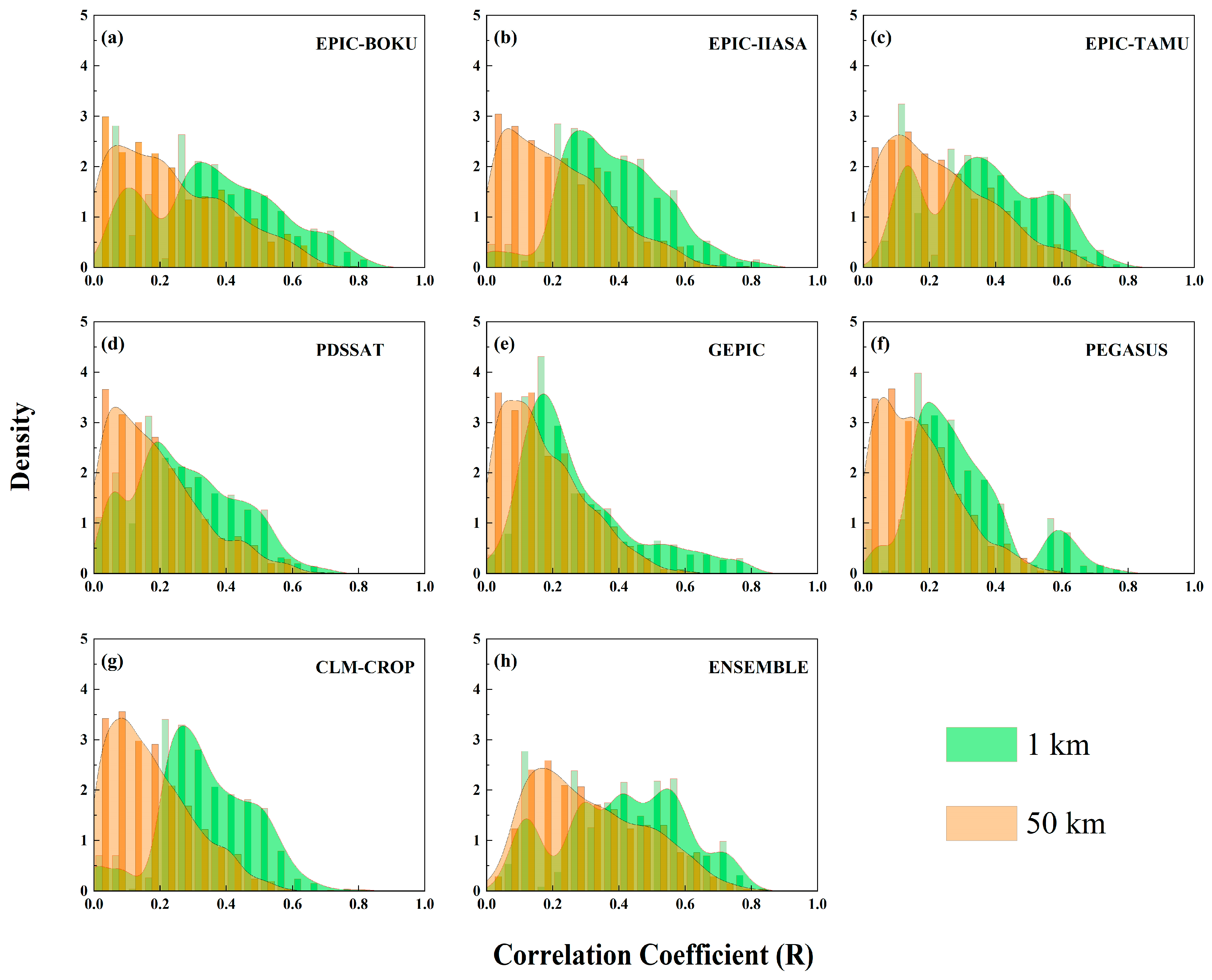
The downscaling models were applied to spatially downscale the county-level maize yield grids simulated by seven GGCMs (EPIC-BOKU, EPIC-TAMU, EPIC-IIASA, GEPIC, PDSSAT, PEGASUS, CLM-CROP) from a 50 km resolution to 1 km for the period of 1980–2010. The ensemble model was created by averaging the outputs of the seven global crop models, and all models were masked using the maize planting area grid provided by MIRCA2000. The data were then aggregated at the county level. Subsequently, we computed the correlation coefficients (R) between the simulated maize yields and the observed maize yields before and after the downscaling process. The density curves in Figure 5 demonstrate a significant improvement in the R values for all crop models after downscaling. The original 50 km-resolution maize yield simulations exhibited R values primarily within the range of 0 to 0.4, signifying poor performance at the county level. Conversely, following downscaling, the R values for the 1 km-resolution maize yield simulations were concentrated within the range of 0.2 to 0.6. This suggests that downscaling effectively enhanced the county-level maize yield simulations for all the GGCMs.
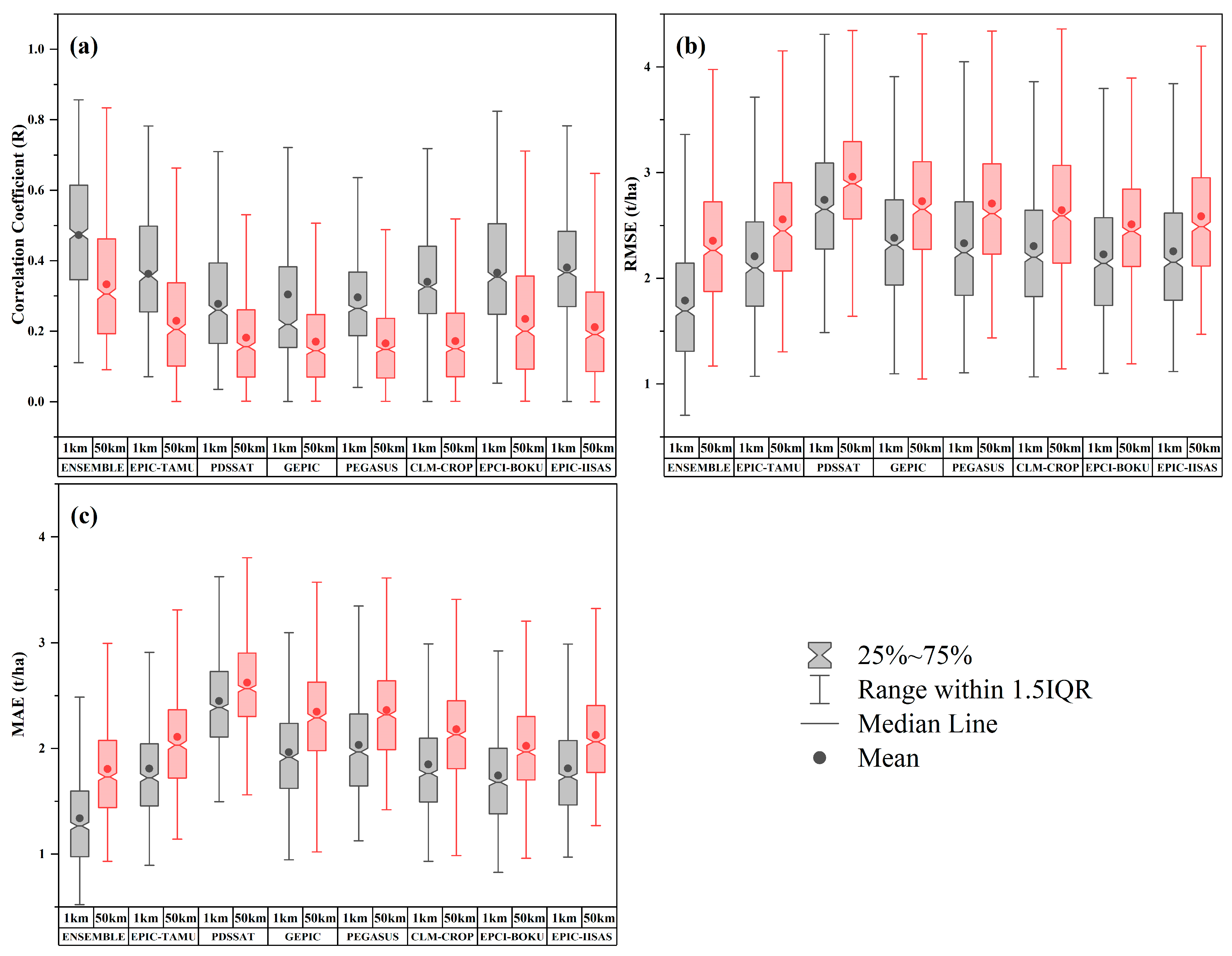
To determine the best-performing model in simulating county-level maize yields in China, we assessed the performance of seven GGCMs before and after downscaling, as well as the ensemble mean of the multi-model, using the indices of R, RMSE, and MAE. The GGCMs demonstrated an improved capacity to elucidate maize yield variability after downscaling (Figure 6). The pre-improvement crop models were only able to explain 16 to 31% of the maize yield variability across a minimum of 1046 counties. However, following improvement, they could explain 30 to 48% of the maize yield variability (average R value across 1046 counties). Simultaneously, both the RMSE and MAE exhibited substantial reductions, with the RMSE decreasing by 0.4 to 0.7 t/ha, and the MAE decreasing by 0.3 to 0.5 t/ha. Among the individual models, EPIC-BOKU performed the best in simulating the county-level maize yield variability (R = 0.38, RMSE = 2.2 t/ha, MAE = 1.7 t/ha), while PDSSAT performed the worst (R = 0.29, RMSE = 2.8 t/ha, MAE = 2.3 t/ha) among the seven models. The multi-model ensemble approach further enhanced the model performance, with ENSEMBLE demonstrating the highest explanatory power for maize yield variability and the lowest errors among all models (R = 0.48, RMSE = 1.8 t/ha, MAE = 1.3 t/ha).
3.3. Evaluation of County-Level Maize Yield Gap in China
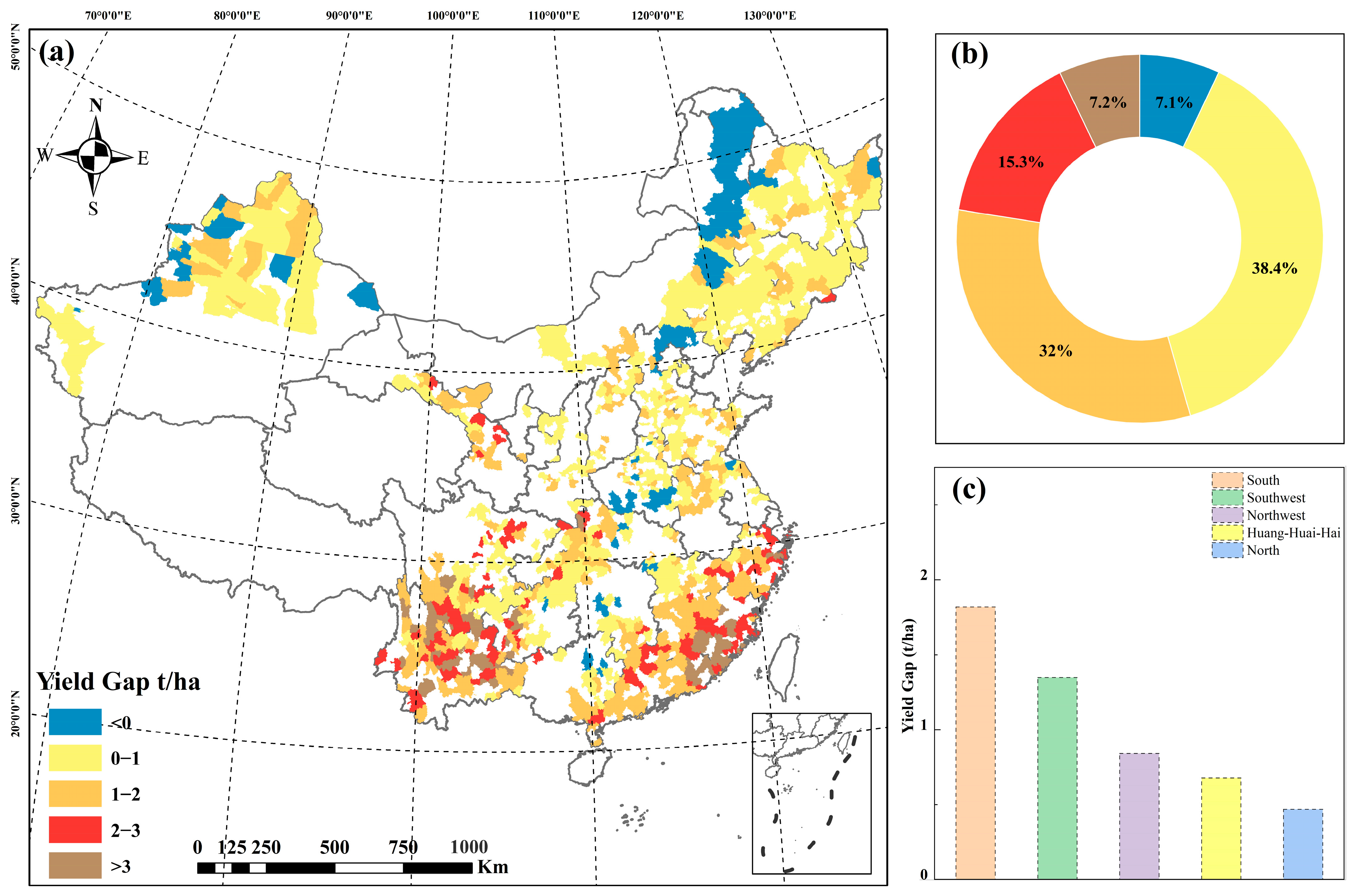
We quantified the maize yield gap in China’s major maize-producing regions (1046 counties). There was still substantial room for improving the maize yield in most counties (Figure 7a). Only 7.1% of all the counties had maize yields that exceeded their potential maize yields, while the remaining 92.9% of counties exhibited room for enhancement in their maize yield (Figure 7b). Counties with maize yield gaps ranging from 0 to 1 t/ha constituted the largest share at 38.4%; counties with maize yield gaps ranging from 1 to 2 t/ha made up 32% of the total; those with maize yield gaps ranging from 2 to 3 t/ha accounted for 15.3% of the counties; and counties with maize yield gaps exceeding 3 t/ha represented a proportion of 7.2%. The spatial distribution pattern indicates that counties with maize yield gaps exceeding 2 t/ha are primarily located in the south and southwest maize regions (Figure 7a). Figure 7c highlights the substantial disparities in the maize yield gaps among different regions, with a substantial average maize yield gap of 1.82 t/ha in the south maize region. The northwest maize region, the Huang-Huai-Hai maize region, and the southwest maize region had maize yield gaps of 0.85 t/ha, 0.65 t/ha, and 1.34 t/ha, respectively. In contrast, the north maize region featured the smallest maize yield gap, at only 0.47 t/ha. These findings emphasize the considerable potential for enhancing maize yields in most counties across China, particularly in the south maize region.
4. Discussion
Among the eight GGCMs models that provided complete configurations for maize yield simulation scenarios, the combination of these models with random forest and multiple data sources yielded outstanding results. Specifically, seven of these models (EPIC-TAMU, EPIC-IIASA, EPIC-BOKU, GEPIC, PDSSAT, PEGASUS, and CLM-CROP) have demonstrated exceptional performance in downscaling simulated maize yields (R2 ≥ 0.9, RMSE < 0.75 t/ha, MAE < 0.5 t/ha). However, due to the use of high-yielding hybrid maize varieties and different maize cultivation practices within PAPSIM, the accuracy of the downscaling models for PAPSIM faced significant challenges [59,60]. Previous studies have shown that GGCMs encounter difficulties in accurately simulating maize yield variability at the county level in China [19]. However, their performance in simulating maize yield variability at the county level in China significantly improved following downscaling, for example, yield variability increased by 14 to 17%, the RMSE decreased by 0.4 to 0.7 t/ha, and the MAE decreased by 0.3 to 0.5 t/ha (Figure 6). The performance of integrated models using the multiple GGCMs (ENSEMBLE, R = 0.48) in our study was found to be very close to that of using the GGCMs for crop yield simulation studies at larger regional scales elsewhere (at the global scale, R = 0.65; at the national scale, R = 0.60; at the provincial scale, R = 0.50) [19,20,61], indicating the increased strength of the model when ensembled. This not only underscores the effectiveness of the downscaling approach but also highlights the potential for more accurate and detailed assessments of crop yield at the county level in China. In comparison to continuously evolving grid-based model simulators, our method significantly improves the computational efficiency and reduces the data processing requirements without sacrificing the simulation performance [62,63]. This allows for a comprehensive assessment of future variations in the yield variability and the associated distribution of extreme yield levels.
When the water supply was insufficient, precipitation and other water-related factors consistently ranked as the most important factors affecting maize yield in China (Figure 4b and Figures S14b–S19b). Temperature and solar radiation were considered the primary factors influencing maize growth only when the maize received adequate irrigation (Figure 4a and Figures S14a–S19a). This reaffirms the predominant influence of precipitation over temperature in determining maize yield variability in most regions [64]. The cumulative or mean climate variables throughout the growing season consistently outweigh the importance of the individual monthly climate variables (Figure 4 and Figures S14–S19). This indicates that the overall levels of high/low temperature, drought, and excessive soil moisture regimes during the maize growing season can significantly impact the maize yield [35,65]. When considering only monthly climate variables, July and August, for example, were found to exert a substantial influence on maize yield in China (Figure 4 and Figures S14–S19), aligning with the notion that climatic conditions during the peak growing period would have been more critical for maize growth [66,67,68]. Interestingly, the importance of soil and topographic features remained consistently low for both the rain-fed and irrigated conditions, possibly due to the inherent insensitivity of GGCMs to soil data [69]. However, despite the low importance of soil and topography, the spatial patterns of maize yield, as shown in Figure 3, indicate that the downscaling model effectively captured information from the soil and topographic data.
Our study has uncovered the untapped potential for maize yields by revealing the maize yield gap in China. In 2010, only 7.1% of the counties achieved their potential maize yield, while the remaining 92.9% still had significant room for increased yields (Figure 7b). Our study also ranked the maize yield gaps in regional China (Figure 7c); the south maize region ranked the highest, and the north maize region ranked the lowest. These rankings of maize yield gaps in regional China can profoundly impact food distribution within the country. Rankings of the maize yield gaps in regional China could also provide a focus in management practices in maize production across different regions. For instance, despite having lower average maize yields, the south maize region exhibited substantial potential for improving their maize yield in the future. One of the contributing factors to the substantially higher maize yield gap in this region is excessive moisture, which can lead to a rapid rate of nitrogen depletion in the soil [17,70,71]. Similarly, the southwest maize region was also found to be affected by excessive moisture availability, experiencing the second-largest yield gaps following the south maize region (Figure 7c) [35,72]. The south maize region and the southwest maize region experienced excessive annual precipitation, leading to soil oversaturation and intense rainfall that could physically damage maize growth [73]. Excessive moisture reduced maize resistance to lodging and nitrogen utilization, impacting regional irrigation, fertilization practices, and soil characteristics [74,75]. Through the optimization of nitrogen management levels, simulated maize yields significantly increased in the south maize region and the southwest maize region (Figure 7c). This indicates that improving nitrogen utilization in these regions can extend the maize planting potential. Our approach used in this study successfully identified maize yield gaps in regional China, and this has become increasingly useful for providing policy strategies to enhance maize yields and reduce yield gaps through better crop management practices, including adequate irrigation, appropriate plantation, and optimized crop fertilization [76,77]. Our findings suggest that China may need to focus on addressing the impact of climate change and improving nitrogen utilization to increase maize yields in the future [72], particularly in the south maize region and the southwest maize region.
The method introduced in this paper demonstrates the tremendous potential of machine learning for building readily applicable downscaling models for GGCMs in spatiotemporal applications. However, certain limitations exist. For instance, the feature variables do not incorporate regional crop management conditions or crop varieties. Crop management conditions often vary based on the local circumstances, and crop varieties need to adapt to regional conditions, such as temperature and precipitation [78]. Therefore, manually combining and systematically training regional crop varieties and management conditions would enhance crop yield simulations at a finer resolution. Additionally, research has shown that remote sensing data can provide supplementary information describing crop growth to further improve crop yield simulations [79,80]. Hence, this could serve as a blueprint for expanding the range and dimensions of feature variables, making the model applicable to a broader range of applications.
5. Conclusions
Our study addresses the important food security issue that China has been facing under rapid climate warming in the 21st century. The advancement of numerical techniques could potentially enhance food security in regional China. In this study, we have demonstrated the effectiveness of integrated machine learning techniques and the downscaling of GGCMs to improve model performance when simulating the county-level maize yield in China. By employing the random forest algorithm with seven GGCMs (EPIC-TAMU, EPIC-IIASA, EPIC-BOKU, GEPIC, PDSSAT, PEGASUS, and CLM-CROP), we have successfully established high-performance downscaled models that can inform China’s crop management practices. We have clearly indicated that the original GGCMs face challenges in accurately simulating county-level maize yields, mainly due to their low spatial resolution, which could only capture approximately 16 to 31% of the yield variability across 1046 counties in China from 1980 to 2010. However, the improved GGCMs significantly enhanced the model performance, explaining 30 to 48% of the maize yield variability at the county level. The model ensemble we made through integration of GGCMs further enhanced the performance and overall accuracy of our results. The maize yield gap quantification we made at the county level in China has successfully revealed that the south maize plantation region has the highest gap, requiring major management attention. We argue that the machine learning approach offers greater spatial advantages for simulations by opening new avenues for the application of GGCMs in regional China and providing valuable insights into improving crop yield simulations.
Supplementary Materials
The following supporting information can be downloaded at: https://www.mdpi.com/article/10.3390/rs16040701/s1, Table S1: Basic introduction to the selected GGCMs. Figure S1: Scatter and density plots for EPIC-IIASA simulations and RF-predicted maize yields in the validation dataset. Notes: “ff” represents the irrigated condition, while “nf” represents the rain-fed condition. (a) Maize yield under irrigated conditions; (b) maize yield under rain-fed conditions; (c) density distribution of maize yield under irrigated conditions; (d) density distribution of maize yield under rain-fed conditions. Figure S2: Scatter and density plots for EPIC-TAMU simulations and RF-predicted maize yields in the validation dataset. Figure S3: Scatter and density plots for PDSSAT simulations and RF-predicted maize yields in the validation dataset. Figure S4: Scatter and density plots for GEPIC simulations and RF-predicted maize yields in the validation dataset. Figure S5: Scatter and density plots for PEGASUS simulations and RF-predicted maize yields in the validation dataset. Figure S6: Scatter and density plots for CLM-CROP simulations and RF-predicted maize yields in the validation dataset. Figure S7: Scatter and density plots for PAPSIM simulations and RF-predicted maize yields in the validation dataset. Figure S8: Spatial distributions of maize yield in China before and after downscaling for EPIC-IIASA. (a) Irrigated maize yield at a spatial resolution of 50 km; (b) irrigated maize yield at a spatial resolution of 1 km; (c) rain-fed maize yield at a spatial resolution of 50 km; and (d) rain-fed maize yield at a spatial resolution of 1 km. Figure S9: Spatial distributions of maize yield in China before and after downscaling for EPIC-TAMU. Figure S10: Spatial distributions of maize yield in China before and after downscaling for PDSSAT. Figure S11: Spatial distributions of maize yield in China before and after downscaling for GEPIC. Figure S12: Spatial distributions of maize yield in China before and after downscaling for PEGASUS. Figure S13: Spatial distributions of maize yield in China before and after downscaling for CLM-CROP. Figure S14: Ranking of feature importance for EPIC-IIASA. (a) Feature importance under irrigated conditions; (b) feature importance under rain-fed conditions. Figure S15: Ranking of feature importance for EPIC-TAMU. Figure S16: Ranking of feature importance for PDSSAT. Figure S17: Ranking of feature importance for GEPIC. Figure S18: Ranking of feature importance for PEGASUS. Figure S19: Ranking of feature importance for CLM-CROP.
Author Contributions
Conceptualization, Y.Z. and L.M.; data curation, Y.Z.; formal analysis, Y.Z.; investigation, Y.Z. and L.M.; methodology, Y.Z.; software, Y.Z.; validation, L.M.; resources, Y.Z.; writing—original draft preparation, Y.Z.; writing—review and editing, G.R.K. and L.M.; visualization, Y.Z.; supervision, L.M.; project administration, Y.Z. and L.M.; funding acquisition, Y.Z. and L.M. All authors have read and agreed to the published version of the manuscript.
Funding
This research was supported by the Postgraduate Research and Practice Innovation Program of Jiangsu Province (KYCX23_1294), the National Natural Science Foundation of China (4210010673), and the Natural Science Foundation of Jiangsu Province (SBK2020040616).
Data Availability Statement
All data resources are provided in the manuscript with links.
Acknowledgments
Yangfeng Zou, Giri Raj Kattel, and Lijuan Miao would like to acknowledge the School of Geographical Sciences, Nanjing University of Information Science and Technology.
Conflicts of Interest
The authors declare no conflicts of interest.
References
- Hunter, M.C.; Smith, R.G.; Schipanski, M.E.; Atwood, L.W.; Mortensen, D.A. Agriculture in 2050: Recalibrating Targets for Sustainable Intensification. BioScience 2017, 67, 386–391. [Google Scholar] [CrossRef]
- Keating, B.A.; Herrero, M.; Carberry, P.S.; Gardner, J.; Cole, M.B. Food wedges: Framing the global food demand and supply challenge towards 2050. Glob. Food Secur. 2014, 3, 125–132. [Google Scholar] [CrossRef]
- Van Dijk, M.; Morley, T.; Rau, M.L.; Saghai, Y. A meta-analysis of projected global food demand and population at risk of hunger for the period 2010–2050. Nat. Food 2021, 2, 494–501. [Google Scholar] [CrossRef]
- Tilman, D.; Balzer, C.; Hill, J.; Befort, B.L. Global food demand and the sustainable intensification of agriculture. Proc. Natl. Acad. Sci. USA 2011, 108, 20260–20264. [Google Scholar] [CrossRef]
- Trnka, M.; Rötter, R.P.; Ruiz-Ramos, M.; Kersebaum, K.C.; Olesen, J.E.; Žalud, Z.; Semenov, M.A. Adverse weather conditions for European wheat production will become more frequent with climate change. Nat. Clim. Chang. 2014, 4, 637–643. [Google Scholar] [CrossRef]
- IPCC. Climate Change and Land: An IPCC Special Report on Climate Change, Desertification, Land Degradation, Sustainable Land Management, Food Security, and Greenhouse Gas Fluxes in Terrestrial Ecosystems. Available online: https://www.ipcc.ch/srccl-report-download-page/ (accessed on 23 August 2019).
- Gomez-Zavaglia, A.; Mejuto, J.C.; Simal-Gandara, J. Mitigation of emerging implications of climate change on food production systems. Food Res. Int. 2020, 134, 109256. [Google Scholar] [CrossRef] [PubMed]
- Godfray, H.C.J.; Beddington, J.R.; Crute, I.R.; Haddad, L.; Lawrence, D.; Muir, J.F.; Pretty, J.; Robinson, S.; Thomas, S.M.; Toulmin, C. Food Security: The Challenge of Feeding 9 Billion People. Science 2010, 327, 812–818. [Google Scholar] [CrossRef] [PubMed]
- Lobell, D.B.; Burke, M.B. On the use of statistical models to predict crop yield responses to climate change. Agric. For. Meteorol. 2010, 150, 1443–1452. [Google Scholar] [CrossRef]
- Zhao, C.; Liu, B.; Piao, S.; Wang, X.; Lobell, D.B.; Huang, Y.; Huang, M.; Yao, Y.; Bassu, S.; Ciais, P.; et al. Temperature increase reduces global yields of major crops in four independent estimates. Proc. Natl. Acad. Sci. USA 2017, 114, 9326–9331. [Google Scholar] [CrossRef] [PubMed]
- Heinicke, S.; Frieler, K.; Jägermeyr, J.; Mengel, M. Global gridded crop models underestimate yield responses to droughts and heatwaves. Environ. Res. Lett. 2022, 17, 044026. [Google Scholar] [CrossRef]
- Mistry, M.N.; Sue Wing, I.; De Cian, E. Simulated vs. empirical weather responsiveness of crop yields: US evidence and implications for the agricultural impacts of climate change. Environ. Res. Lett. 2017, 12, 075007. [Google Scholar] [CrossRef]
- Rosenzweig, C.; Elliott, J.; Deryng, D.; Ruane, A.C.; Müller, C.; Arneth, A.; Boote, K.J.; Folberth, C.; Glotter, M.; Khabarov, N.; et al. Assessing agricultural risks of climate change in the 21st century in a global gridded crop model intercomparison. Proc. Natl. Acad. Sci. USA 2014, 111, 3268–3273. [Google Scholar] [CrossRef] [PubMed]
- Rosenzweig, C.; Jones, J.W.; Hatfield, J.L.; Ruane, A.C.; Boote, K.J.; Thorburn, P.; Antle, J.M.; Nelson, G.C.; Porter, C.; Janssen, S.; et al. The Agricultural Model Intercomparison and Improvement Project (AgMIP): Protocols and pilot studies. Agric. For. Meteorol. 2013, 170, 166–182. [Google Scholar] [CrossRef]
- Warszawski, L.; Frieler, K.; Huber, V.; Piontek, F.; Serdeczny, O.; Schewe, J. The Inter-Sectoral Impact Model Intercomparison Project (ISI–MIP): Project framework. Proc. Natl. Acad. Sci. USA 2014, 111, 3228–3232. [Google Scholar] [CrossRef] [PubMed]
- Elliott, J.; Müller, C.; Deryng, D.; Chryssanthacopoulos, J.; Boote, K.J.; Büchner, M.; Foster, I.; Glotter, M.; Heinke, J.; Iizumi, T.; et al. The Global Gridded Crop Model Intercomparison: Data and modeling protocols for Phase 1 (v1.0). Geosci. Model Dev. 2015, 8, 261–277. [Google Scholar] [CrossRef]
- Folberth, C.; Elliott, J.; Müller, C.; Balkovic, J.; Chryssanthacopoulos, J.; Izaurralde, R.C.; Jones, C.D.; Khabarov, N.; Liu, W.; Reddy, A.; et al. Uncertainties in global crop model frameworks: Effects of cultivar distribution, crop management and soil handling on crop yield estimates. Biogeosciences Discuss. 2016, 2016, 1–30. [Google Scholar] [CrossRef]
- Van Meijl, H.; Havlik, P.; Lotze-Campen, H.; Stehfest, E.; Witzke, P.; Domínguez, I.P.; Bodirsky, B.L.; van Dijk, M.; Doelman, J.; Fellmann, T.; et al. Comparing impacts of climate change and mitigation on global agriculture by 2050. Environ. Res. Lett. 2018, 13, 064021. [Google Scholar] [CrossRef]
- Yin, X.; Leng, G. Modelling global impacts of climate variability and trend on maize yield during 1980–2010. Int. J. Climatol. 2021, 41, E1583–E1596. [Google Scholar] [CrossRef]
- Li, Z.; Zhan, C.; Hu, S.; Ning, L.; Wu, L.; Guo, H. Evaluation of global gridded crop models (GGCMs) for the simulation of major grain crop yields in China. Hydrol. Res. 2022, 53, 353–369. [Google Scholar] [CrossRef]
- Folberth, C.; Baklanov, A.; Balkovič, J.; Skalský, R.; Khabarov, N.; Obersteiner, M. Spatio-temporal downscaling of gridded crop model yield estimates based on machine learning. Agric. For. Meteorol. 2019, 264, 1–15. [Google Scholar] [CrossRef]
- Reidsma, P.; Ewert, F.; Boogaard, H.; Diepen, K.v. Regional crop modelling in Europe: The impact of climatic conditions and farm characteristics on maize yields. Agric. Syst. 2009, 100, 51–60. [Google Scholar] [CrossRef]
- Ewert, F.; van Ittersum, M.K.; Heckelei, T.; Therond, O.; Bezlepkina, I.; Andersen, E. Scale changes and model linking methods for integrated assessment of agri-environmental systems. Agric. Ecosyst. Environ. 2011, 142, 6–17. [Google Scholar] [CrossRef]
- Rosenzweig, C.; Ruane, A.C.; Antle, J.; Elliott, J.; Ashfaq, M.; Chatta, A.A.; Ewert, F.; Folberth, C.; Hathie, I.; Havlik, P.; et al. Coordinating AgMIP data and models across global and regional scales for 1.5 °C and 2.0 °C assessments. Philos. Trans. R. Soc. A Math. Phys. Eng. Sci. 2018, 376, 20160455. [Google Scholar] [CrossRef]
- Prodhan, F.A.; Zhang, J.; Pangali Sharma, T.P.; Nanzad, L.; Zhang, D.; Seka, A.M.; Ahmed, N.; Hasan, S.S.; Hoque, M.Z.; Mohana, H.P. Projection of future drought and its impact on simulated crop yield over South Asia using ensemble machine learning approach. Sci. Total Environ. 2022, 807, 151029. [Google Scholar] [CrossRef] [PubMed]
- Li, X.; Fang, S.; Wu, D.; Zhu, Y.; Wu, Y. Risk analysis of maize yield losses in mainland China at the county level. Sci. Rep. 2020, 10, 10684. [Google Scholar] [CrossRef]
- Ruane, A.C.; Goldberg, R.; Chryssanthacopoulos, J. Climate forcing datasets for agricultural modeling: Merged products for gap-filling and historical climate series estimation. Agric. For. Meteorol. 2015, 200, 233–248. [Google Scholar] [CrossRef]
- Witten, I.H.; Frank, E. Data mining: Practical machine learning tools and techniques with Java implementations. ACM SIGMOD Rec. 2002, 31, 76–77. [Google Scholar] [CrossRef]
- Yang, P.; Zhao, Q.; Cai, X. Machine learning based estimation of land productivity in the contiguous US using biophysical predictors. Environ. Res. Lett. 2020, 15, 074013. [Google Scholar] [CrossRef]
- Mohanasundaram, S.; Kasiviswanathan, K.S.; Purnanjali, C.; Santikayasa, I.P.; Singh, S. Downscaling Global Gridded Crop Yield Data Products and Crop Water Productivity Mapping Using Remote Sensing Derived Variables in the South Asia. Int. J. Plant Prod. 2023, 17, 1–16. [Google Scholar] [CrossRef]
- Duro, D.C.; Franklin, S.E.; Dubé, M.G. A comparison of pixel-based and object-based image analysis with selected machine learning algorithms for the classification of agricultural landscapes using SPOT-5 HRG imagery. Remote Sens. Environ. 2012, 118, 259–272. [Google Scholar] [CrossRef]
- Shin, J.-Y.; Kim, K.R.; Ha, J.-C. Seasonal forecasting of daily mean air temperatures using a coupled global climate model and machine learning algorithm for field-scale agricultural management. Agric. For. Meteorol. 2020, 281, 107858. [Google Scholar] [CrossRef]
- Shahhosseini, M.; Hu, G.; Huber, I.; Archontoulis, S.V. Coupling machine learning and crop modeling improves crop yield prediction in the US Corn Belt. Sci. Rep. 2021, 11, 1606. [Google Scholar] [CrossRef]
- Yang, Y.; Xu, W.; Hou, P.; Liu, G.; Liu, W.; Wang, Y.; Zhao, R.; Ming, B.; Xie, R.; Wang, K.; et al. Improving maize grain yield by matching maize growth and solar radiation. Sci. Rep. 2019, 9, 3635. [Google Scholar] [CrossRef]
- Liu, W.; Li, Z.; Li, Y.; Ye, T.; Chen, S.; Liu, Y. Heterogeneous impacts of excessive wetness on maize yields in China: Evidence from statistical yields and process-based crop models. Agric. For. Meteorol. 2022, 327, 109205. [Google Scholar] [CrossRef]
- Butler, E.E.; Huybers, P. Adaptation of US maize to temperature variations. Nat. Clim. Chang. 2013, 3, 68–72. [Google Scholar] [CrossRef]
- Liu, H.; Zhang, X.; Wang, Y.; Guo, Y.; Shen, Y. Spatio-temporal characteristics of the hydrothermal conditions in the growth period and various gro wth stages of maize in China from 1960 to 2018. Chin. J. Eco-Agric. 2021, 29, 1417–1429. [Google Scholar] [CrossRef]
- Müller, C.; Elliott, J.; Chryssanthacopoulos, J.; Deryng, D.; Folberth, C.; Pugh, T.A.M.; Schmid, E. Implications of climate mitigation for future agricultural production. Environ. Res. Lett. 2015, 10, 125004. [Google Scholar] [CrossRef]
- Gelaro, R.; McCarty, W.; Suárez, M.J.; Todling, R.; Molod, A.; Takacs, L.; Randles, C.A.; Darmenov, A.; Bosilovich, M.G.; Reichle, R.; et al. The Modern-Era Retrospective Analysis for Research and Applications, Version 2 (MERRA-2). J. Clim. 2017, 30, 5419–5454. [Google Scholar] [CrossRef] [PubMed]
- Wieder, W. Regridded Harmonized World Soil Database v1.2; Oak Ridge National Laboratory: Roane County, TN, USA, 2014. [Google Scholar] [CrossRef]
- Gandhi, S.M.; Sarkar, B.C. Chapter 3—Reconnaissance and Prospecting. In Essentials of Mineral Exploration and Evaluation; Gandhi, S.M., Sarkar, B.C., Eds.; Elsevier: Amsterdam, The Netherlands, 2016; pp. 53–79. [Google Scholar]
- Portmann, F.T.; Siebert, S.; Döll, P. MIRCA2000—Global monthly irrigated and rainfed crop areas around the year 2000: A new high-resolution data set for agricultural and hydrological modeling. Glob. Biogeochem. Cycles. 2010, 24, 24. [Google Scholar] [CrossRef]
- Ray, D.K.; Ramankutty, N.; Mueller, N.D.; West, P.C.; Foley, J.A. Recent patterns of crop yield growth and stagnation. Nat. Commun. 2012, 3, 1293. [Google Scholar] [CrossRef]
- Müller, C.; Elliott, J.; Chryssanthacopoulos, J.; Arneth, A.; Balkovic, J.; Ciais, P.; Deryng, D.; Folberth, C.; Glotter, M.; Hoek, S.; et al. Global gridded crop model evaluation: Benchmarking, skills, deficiencies and implications. Geosci. Model Dev. 2017, 10, 1403–1422. [Google Scholar] [CrossRef]
- Lobell, D.B.; Field, C.B. Global scale climate–crop yield relationships and the impacts of recent warming. Environ. Res. Lett. 2007, 2, 014002. [Google Scholar] [CrossRef]
- Villoria, N.B.; Elliott, J.; Müller, C.; Shin, J.; Zhao, L.; Song, C. Rapid aggregation of global gridded crop model outputs to facilitate cross-disciplinary analysis of climate change impacts in agriculture. Environ. Model. Softw. 2016, 75, 193–201. [Google Scholar] [CrossRef]
- Porwollik, V.; Müller, C.; Elliott, J.; Chryssanthacopoulos, J.; Iizumi, T.; Ray, D.K.; Ruane, A.C.; Arneth, A.; Balkovič, J.; Ciais, P.; et al. Spatial and temporal uncertainty of crop yield aggregations. Eur. J. Agron. 2017, 88, 10–21. [Google Scholar] [CrossRef]
- Breiman, L. Random Forests. Mach. Learn. 2001, 45, 5–32. [Google Scholar] [CrossRef]
- Elavarasan, D.; Vincent, D.R.; Sharma, V.; Zomaya, A.Y.; Srinivasan, K. Forecasting yield by integrating agrarian factors and machine learning models: A survey. Comput. Electron. Agric. 2018, 155, 257–282. [Google Scholar] [CrossRef]
- Cai, Y.; Guan, K.; Peng, J.; Wang, S.; Seifert, C.; Wardlow, B.; Li, Z. A high-performance and in-season classification system of field-level crop types using time-series Landsat data and a machine learning approach. Remote Sens. Environ. 2018, 210, 35–47. [Google Scholar] [CrossRef]
- Strobl, C.; Boulesteix, A.-L.; Zeileis, A.; Hothorn, T. Bias in random forest variable importance measures: Illustrations, sources and a solution. BMC Bioinform. 2007, 8, 25. [Google Scholar] [CrossRef] [PubMed]
- Zhang, L.; Zhang, Z.; Luo, Y.; Cao, J.; Tao, F. Combining Optical, Fluorescence, Thermal Satellite, and Environmental Data to Predict County-Level Maize Yield in China Using Machine Learning Approaches. Remote Sens. 2020, 12, 21. [Google Scholar] [CrossRef]
- Li, M.; Zhao, J.; Yang, X. Building a new machine learning-based model to estimate county-level climatic yield variation for maize in Northeast China. Comput. Electron. Agric. 2021, 191, 106557. [Google Scholar] [CrossRef]
- Roy, M.-H.; Larocque, D. Robustness of random forests for regression. J. Nonparametric Stat. 2012, 24, 993–1006. [Google Scholar] [CrossRef]
- Li, Z.; Zhang, Z.; Zhang, L. Improving regional wheat drought risk assessment for insurance application by integrating scenario-driven crop model, machine learning, and satellite data. Agric. Syst. 2021, 191, 103141. [Google Scholar] [CrossRef]
- Li, L.; Zhang, Y.; Wang, B.; Feng, P.; He, Q.; Shi, Y.; Liu, K.; Harrison, M.T.; Liu, D.L.; Yao, N.; et al. Integrating machine learning and environmental variables to constrain uncertainty in crop yield change projections under climate change. Eur. J. Agron. 2023, 149, 126917. [Google Scholar] [CrossRef]
- Luo, Y.; Zhang, Z.; Chen, Y.; Li, Z.; Tao, F. ChinaCropPhen1km: A high-resolution crop phenological dataset for three staple crops in China during 2000–2015 based on leaf area index (LAI) products. Earth Syst. Sci. Data 2020, 12, 197–214. [Google Scholar] [CrossRef]
- Liu, Y.; Qin, Y.; Ge, Q. Spatiotemporal differentiation of changes in maize phenology in China from 1981 to 2010. J. Geogr. Sci. 2019, 29, 351–362. [Google Scholar] [CrossRef]
- Keating, B.A.; Carberry, P.S.; Hammer, G.L.; Probert, M.E.; Robertson, M.J.; Holzworth, D.; Huth, N.I.; Hargreaves, J.N.G.; Meinke, H.; Hochman, Z.; et al. An overview of APSIM, a model designed for farming systems simulation. Eur. J. Agron. 2003, 18, 267–288. [Google Scholar] [CrossRef]
- Müller, C.; Elliott, J.; Kelly, D.; Arneth, A.; Balkovic, J.; Ciais, P.; Deryng, D.; Folberth, C.; Hoek, S.; Izaurralde, R.C.; et al. The Global Gridded Crop Model Intercomparison phase 1 simulation dataset. Sci. Data 2019, 6, 50. [Google Scholar] [CrossRef] [PubMed]
- Ringeval, B.; Müller, C.; Pugh, T.A.M.; Mueller, N.D.; Ciais, P.; Folberth, C.; Liu, W.; Debaeke, P.; Pellerin, S. Potential yield simulated by global gridded crop models: Using a process-based emulator to explain their differences. Geosci. Model Dev. 2021, 14, 1639–1656. [Google Scholar] [CrossRef]
- Franke, J.A.; Müller, C.; Elliott, J.; Ruane, A.C.; Jägermeyr, J.; Snyder, A.; Dury, M.; Falloon, P.D.; Folberth, C.; François, L.; et al. The GGCMI Phase 2 emulators: Global gridded crop model responses to changes in CO2, temperature, water, and nitrogen (version 1.0). Geosci. Model Dev. 2020, 13, 3995–4018. [Google Scholar] [CrossRef]
- Blanc, É. Statistical emulators of maize, rice, soybean and wheat yields from global gridded crop models. Agric. For. Meteorol. 2017, 236, 145–161. [Google Scholar] [CrossRef]
- Frieler, K.; Schauberger, B.; Arneth, A.; Balkovič, J.; Chryssanthacopoulos, J.; Deryng, D.; Elliott, J.; Folberth, C.; Khabarov, N.; Müller, C.; et al. Understanding the weather signal in national crop-yield variability. Earth's Future 2017, 5, 605–616. [Google Scholar] [CrossRef]
- Zhu, X.; Xu, K.; Liu, Y.; Guo, R.; Chen, L. Assessing the vulnerability and risk of maize to drought in China based on the AquaCrop model. Agric. Syst. 2021, 189, 103040. [Google Scholar] [CrossRef]
- Benincasa, P.; Reale, L.; Tedeschini, E.; Ferri, V.; Cerri, M.; Ghitarrini, S.; Falcinelli, B.; Frenguelli, G.; Ferranti, F.; Ayano, B.E.; et al. The relationship between grain and ovary size in wheat: An analysis of contrasting grain weight cultivars under different growing conditions. Field Crops Res. 2017, 210, 175–182. [Google Scholar] [CrossRef]
- Kim, N.; Lee, Y.-W. Machine Learning Approaches to Corn Yield Estimation Using Satellite Images and Climate Data: A Case of Iowa State. J. Korean Soc. Surv. Geodesy Photogramm. Cartogr. 2016, 34, 383–390. [Google Scholar] [CrossRef]
- Zhao, Y.; Lobell, D.B. Assessing the heterogeneity and persistence of farmers’ maize yield performance across the North China Plain. Field Crops Res. 2017, 205, 55–66. [Google Scholar] [CrossRef]
- Folberth, C.; Skalský, R.; Moltchanova, E.; Balkovič, J.; Azevedo, L.B.; Obersteiner, M.; van der Velde, M. Uncertainty in soil data can outweigh climate impact signals in global crop yield simulations. Nat. Commun. 2016, 7, 11872. [Google Scholar] [CrossRef] [PubMed]
- Lobell, D.B.; Deines, J.M.; Tommaso, S.D. Changes in the drought sensitivity of US maize yields. Nat. Food 2020, 1, 729–735. [Google Scholar] [CrossRef] [PubMed]
- Lesk, C.; Coffel, E.; Horton, R. Net benefits to US soy and maize yields from intensifying hourly rainfall. Nat. Clim. Chang. 2020, 10, 819–822. [Google Scholar] [CrossRef]
- Yu, Y.; Jiang, Z.; Wang, G.; Kattel, G.R.; Chuai, X.; Shang, Y.; Zou, Y.; Miao, L. Disintegrating the impact of climate change on maize yield from human management practices in China. Agric. For. Meteorol. 2022, 327, 109235. [Google Scholar] [CrossRef]
- Li, Y.; Guan, K.; Schnitkey, G.D.; DeLucia, E.; Peng, B. Excessive rainfall leads to maize yield loss of a comparable magnitude to extreme drought in the United States. Glob. Chang. Biol. 2019, 25, 2325–2337. [Google Scholar] [CrossRef] [PubMed]
- Haqiqi, I.; Grogan, D.S.; Hertel, T.W.; Schlenker, W. Quantifying the impacts of compound extremes on agriculture. Hydrol. Earth Syst. Sci. 2021, 25, 551–564. [Google Scholar] [CrossRef]
- Lu, Y.; Wang, E.; Zhao, Z.; Liu, X.; Tian, A.; Zhang, X. Optimizing irrigation to reduce N leaching and maintain high crop productivity through the manipulation of soil water storage under summer monsoon climate. Field Crops Res. 2021, 265, 108110. [Google Scholar] [CrossRef]
- Cui, Z.; Chen, X.; Miao, Y.; Zhang, F.; Sun, Q.; Schroder, J.; Zhang, H.; Li, J.; Shi, L.; Xu, J.; et al. On-Farm Evaluation of the Improved Soil Nmin–based Nitrogen Management for Summer Maize in North China Plain. Agron. J. 2008, 100, 517–525. [Google Scholar] [CrossRef]
- Chlingaryan, A.; Sukkarieh, S.; Whelan, B. Machine learning approaches for crop yield prediction and nitrogen status estimation in precision agriculture: A review. Comput. Electron. Agric. 2018, 151, 61–69. [Google Scholar] [CrossRef]
- Jin, Z.; Azzari, G.; Burke, M.; Aston, S.; Lobell, D.B. Mapping Smallholder Yield Heterogeneity at Multiple Scales in Eastern Africa. Remote Sens. 2017, 9, 931. [Google Scholar] [CrossRef]
- Zhou, W.; Liu, Y.; Ata-Ul-Karim, S.T.; Ge, Q.; Li, X.; Xiao, J. Integrating climate and satellite remote sensing data for predicting county-level wheat yield in China using machine learning methods. Int. J. Appl. Earth Obs. Geoinf. 2022, 111, 102861. [Google Scholar] [CrossRef]
- Cai, Y.; Guan, K.; Lobell, D.; Potgieter, A.B.; Wang, S.; Peng, J.; Xu, T.; Asseng, S.; Zhang, Y.; You, L.; et al. Integrating satellite and climate data to predict wheat yield in Australia using machine learning approaches. Agric. For. Meteorol. 2019, 274, 144–159. [Google Scholar] [CrossRef]
Figure 1.
The five maize planting regions in China. Notes: Zone I: the north maize region; Zone II: the Huang-Huai-Hai maize region; Zone III: the southwest maize region; Zone IV: the northwest maize region; and Zone V: the south maize region.
Figure 1.
The five maize planting regions in China. Notes: Zone I: the north maize region; Zone II: the Huang-Huai-Hai maize region; Zone III: the southwest maize region; Zone IV: the northwest maize region; and Zone V: the south maize region.

Figure 2.
Scatter and density plots for GGCM simulations and RF-predicted maize yields in the validation dataset. Taking EPIC-BOKU as an example, the other models are detailed in the Supplementary Materials (Figures S1–S7). Notes: “ff” represents the irrigated condition, while “nf” represents the rain-fed condition. (a) Maize yield under irrigated conditions; (b) maize yield under rain-fed conditions; (c) density distribution of maize yield under irrigated conditions; (d) density distribution of maize yield under rain-fed conditions.

Figure 3.
Spatial distributions of maize yield in China before and after downscaling. Taking EPIC-BOKU as an example, the other models are detailed in the Supplementary Materials (Figures S8–S13). (a) Irrigated maize yield at a spatial resolution of 50 km; (b) irrigated maize yield at a spatial resolution of 1 km; (c) rain-fed maize yield at a spatial resolution of 50 km; and (d) rain-fed maize yield at a spatial resolution of 1 km.

Figure 4.
Ranking of feature importance. Taking EPIC-BOKU as an example, the other models are detailed in the Supplementary Materials (Figures S14–S19). (a) Feature importance under irrigated conditions; (b) feature importance under rain-fed conditions.
Figure 4.
Ranking of feature importance. Taking EPIC-BOKU as an example, the other models are detailed in the Supplementary Materials (Figures S14–S19). (a) Feature importance under irrigated conditions; (b) feature importance under rain-fed conditions.

Figure 5.
Density distribution of the correlation coefficients between 1 km-resolution simulated maize yields and 50 km-resolution simulated maize yields, in comparison to maize yield observations in China from 1980 to 2010. (a) Density distribution of EPIC-BOKU; (b) density distribution of EPIC-IIASA; (c) density distribution of EPIC-TAMU; (d) density distribution of PDSSAT; (e) density distribution of GEPIC; (f) density distribution of PEGASUS; (g) density distribution of CLM-CROP; (h) density distribution of ENSEMBLE.

Figure 6.
The performance of GGCMs’ simulated maize yields before and after downscaling. (a) The correlation coefficient (R) between simulated maize yields and observed county-level maize yields before and after downscaling; (b) the root mean square error (RMSE) between simulated maize yields and observed county-level maize yields before and after downscaling; (c) the mean absolute error (MAE) between simulated maize yields and observed county-level maize yields before and after downscaling. Notes: Red represents GGCMs before downscaling (50 km); brown represents GGCMs after downscaling (1 km).

Figure 7.
Maize yield disparity at the county level in China. (a) Maize yield gaps in various counties; (b) percentage of counties falling into each interval (<0 t/ha, 0–1 t/ha, 1–2 t/ha, 2–3 t/ha, >3 t/ha); (c) average maize yield discrepancy across five maize plantation regions in China (the south maize region, the southwest maize region, the northeast maize region, the Huang-Huai-Hai maize region, and the northwest maize region).


Table 1.
Features and target variables for machine learning.
| Variables | Variable Descriptions |
|---|---|
| Climate variables (VARs) | |
| TMAX | Maximum temperature (°C) |
| TMIN | Minimum temperature (°C) |
| TAVG | Average temperature (°C) |
| PRATE | Total precipitation (mm) |
| SRAD | Solar radiation (MJ/m2) |
| PET | Potential evapotranspiration (mm) |
| WS | Wind speed (m/s) |
| VPD | Vapor pressure deficit (h PA) |
| Temporal aggregates of climate variables | |
| VAR_X | Monthly value for month X in calendar year (e.g., “TMAX_1”) |
| VARsumGS | Sum of climate variables in growing season (e.g., “TMAXsumGS”) |
| VARavgGS | Average of climate variables in growing season (e.g., “TMAXavgGS”) |
| Soil and topography variables | |
| DEPTH | Total soil depth (m) |
| OC | Organic carbon content in topsoil (%) |
| SAND | Sand content in topsoil (%) |
| SB | Sum of bases in topsoil (cmol/kg) |
| ROK | Coarse fragment (rock) content in topsoil (%) |
| CLAY | Clay content in topsoil (%) |
| EC | Electric conductivity in topsoil (mmho/cm) |
| BD | Bulk density in topsoil (g/cm3) |
| CEC | Cation exchange capacity in topsoil (cmol/kg) |
| PH | pH in topsoil |
| CARB | Carbonate content in topsoil (%) |
| DEM | Digital elevation model |
| Target variables | |
| YIELD | Simulated maize yield (t/ha) |
Disclaimer/Publisher’s Note: The statements, opinions and data contained in all publications are solely those of the individual author(s) and contributor(s) and not of MDPI and/or the editor(s). MDPI and/or the editor(s) disclaim responsibility for any injury to people or property resulting from any ideas, methods, instructions or products referred to in the content. |
© 2024 by the authors. Licensee MDPI, Basel, Switzerland. This article is an open access article distributed under the terms and conditions of the Creative Commons Attribution (CC BY) license (https://creativecommons.org/licenses/by/4.0/).
Share and Cite
MDPI and ACS Style
Zou, Y.; Kattel, G.R.; Miao, L. Enhancing Maize Yield Simulations in Regional China Using Machine Learning and Multi-Data Resources. Remote Sens. 2024, 16, 701. https://doi.org/10.3390/rs16040701
AMA Style
Zou Y, Kattel GR, Miao L. Enhancing Maize Yield Simulations in Regional China Using Machine Learning and Multi-Data Resources. Remote Sensing. 2024; 16(4):701. https://doi.org/10.3390/rs16040701
Chicago/Turabian StyleZou, Yangfeng, Giri Raj Kattel, and Lijuan Miao. 2024. "Enhancing Maize Yield Simulations in Regional China Using Machine Learning and Multi-Data Resources" Remote Sensing 16, no. 4: 701. https://doi.org/10.3390/rs16040701
Note that from the first issue of 2016, this journal uses article numbers instead of page numbers. See further details here.