

Abstract
Extreme events can lead to crop yield declines, resulting in financial losses and threats to food security, and the frequency and intensity of such events is projected to increase. As global gridded crop models (GGCMs) are commonly used to assess climate change impacts on agricultural yields, there is a need to understand whether these models are able to reproduce the observed yield declines. We evaluated 13 GGCMs from the Inter-Sectoral Impact Model Intercomparison Project and compared observed and simulated impact of past droughts and heatwaves on yields for four crops (maize, rice, soy, wheat). We found that most models detect but underestimate the impact of droughts and heatwaves on yield. Specifically, the drought signal was detected by 12 of 13 models for maize and all models for wheat, while the heat signal was detected by eleven models for maize and six models for wheat. To investigate whether the difference between simulated and observed yield declines is due to a misrepresentation of simulated exposure to heat or water scarcity (i.e. misrepresentation of growing season), we analysed the relationship between average discrepancies between observed and simulated yield losses, and average simulated exposure to extreme weather conditions across all crop models. We found a positive correlation between simulated exposure to heat and model performance for heatwaves, but found no correlation for droughts. This suggests that there is a systematic underestimation of yield responses to heat and drought and not only a misrepresentation of exposure. Assuming that performance for the past indicates models' capacity to project future yield impacts, models likely underestimate future yield decline from climate change. High-quality temporally and spatially resolved observational data on growing seasons will be highly valuable to further improve crop models' capacity to adequately respond to extreme weather events.
Export citation and abstract BibTeX RIS

Original content from this work may be used under the terms of the Creative Commons Attribution 4.0 license. Any further distribution of this work must maintain attribution to the author(s) and the title of the work, journal citation and DOI.
1. Introduction
Crop yields are strongly impacted by weather conditions (Frieler et al 2017, Müller et al 2017, FAO 2018). Especially extreme weather events, such as droughts and heatwaves, can have detrimental impacts on crop yields (Lesk et al 2016). Yield variability in turn affects food supply and prices (FAO 2018), and ultimately livelihoods of farmers and those consumers that spend a large proportion of their income on food. As more than 20% of food is traded internationally (D'Odorico et al 2014), local production shocks can have global impacts especially for countries relying on food imports, such as during the 2008/2010 spike in food prices (Maetz et al 2011).
Over the last decades, the frequency and strength of extreme weather events increased substantially, and this trend will likely continue (Morales et al 2020, Perkins-Kirkpatrick and Lewis 2020). In addition, the likelihood of multiple regions being affected at the same time is increasing, which could exacerbate negative impacts on agricultural production (Gaupp et al 2020). To inform agricultural practices, spatial planning, or the development of insurance policies for farmers, there is a need to better understand yield responses to weather disturbances to improve future projections under climate change.
Global gridded crop models (GGCMs) have been developed to assess how climate change and agricultural management might impact crop yields (Müller et al 2017, Jägermeyr et al 2021). To enable model intercomparison the Agricultural Model Intercomparison and Improvement Project (AgMIP) and the Inter-Sectoral Impact Model Intercomparison Project (ISIMIP) provide common modelling protocols describing a harmonized simulation setup. It has been tested how much of the annual variability of crop yields can be explained by weather fluctuations with strong differences in performance between countries, crops and models (Frieler et al 2017, Müller et al 2017, 2019). Given high explanatory power in some regions, an unresolved question is to what extent lower model performance in other regions is due to a misrepresentation of how crops respond to heat stress and drought conditions, or due to a misrepresentation of management practices including planting and harvest dates (Rötter et al 2011). Concerning the response to extreme temperature, Schauberger et al (2017) found that GGCMs reproduce yield decline observed under temperatures above 30 °C. Regarding management practices, Jägermeyr and Frieler (2018) showed that observed yield declines under droughts and heatwaves can be reproduced with a gridded global crop model (LPJmL) after constraining the growing seasons in the model by observations, i.e. heat units required to reach maturity. An analysis of GGCM performance for the 2003 European heatwave found that inadequate consideration of management practices likely resulted in the poor performance of models for some countries (Schewe et al 2019).
In this study, we expand the evaluation of GGCMs to all AgMIP-ISIMIP2a models in terms of model performance for simulating national yield anomalies, and the impact of drought and heatwaves on yield from 1971 to 2012. We also analysed to what extent model performance is influenced by the growing season representation in the model.
2. Methods
2.1. ISIMIP crop models
We compared crop yield models that were run by 13 modelling groups as part of the AgMIP-ISIMIP2a simulation round: CGMS-WOFOST, CLM-Crop, EPIC-Boku, EPIC-IIASA, EPIC-TAMU, GEPIC, LPJ-GUESS, LPJmL, ORCHIDEE-CROP, pAPSIM, pDSSAT, PEGASUS, and PEPIC (Arneth et al 2017). For a basic characterization of the models see Müller et al (2019) and www.isimip.org/impactmodels. The models are forced by four observational climate datasets in daily resolution, namely GSWP3, Princeton, WATCH, and WFDEI. The original simulations do not account for land-use patterns but are executed as 'pure crop runs' on a 0.5° × 0.5° grid assuming that the considered crop is grown in each terrestrial grid cell with suitable weather and soil conditions, based on the soil map from Harmonized World Soil Database (www.isimip.org/protocol). Crop yield is defined as harvested production per unit of harvested area and is reported per annual growing season. Yields were multiplied by land-use and irrigation patterns in annual resolution to derive production per grid cell. Land-use and irrigation data were taken from 'Dynamic MIRCA' based on HYDE (Klein Goldewijk et al 2017) and MIRCA2000 (Portmann et al 2010) as provided by ISIMIP2a. Mean national yields are calculated by dividing total national production by the total (rainfed + irrigated) harvested area. Two irrigation setups are simulated: (a) purely rainfed conditions and (b) full irrigation avoiding water stress without accounting for potential limitations in water availability.
The crop models simulated four crops (maize, rice, soy, and wheat), and two nitrogen application settings ('default' and 'fullharm'). Default runs used model specific best-guess representations of historical fertilizer inputs, if the model is capable, and their default growing season representation, either as model-estimated planting dates or individual input dataset. Full harmonization (fullharm) runs used prescribed annual fertilizer application rates, planting and harvest dates (Müller et al 2017). To meet the prescribed harvest dates on average, the models are calibrated to meet the required heat units to reach maturity in each grid cell. Not all modelling groups ran all combinations of crops, scenarios and climate datasets. This analysis included 67 model runs for maize, 59 for rice, 66 for soy and 70 for wheat (table S2 available online at stacks.iop.org/ERL/17/044026/mmedia).
2.2. Inter-annual variability in national yields
The historical evolution of crop yields is strongly influenced by technical progress leading to increases in yields that are not necessarily captured by crop models. Therefore, national time series of simulated and observed crop yields were de-trended by subtracting a quadratic temporal trend. In order to measure the degree to which models reproduce the variations in observed yields, we calculated the root mean squared error (RMSE) and the explained variance (R2) between simulated and observed yield anomaly based on the Pearson correlation coefficient. Depending on the harvest date, there can be difficulties in attributing growing periods to calendar years and Food and Agriculture Organization of the United Nations (FAO) data reporting. Thus, we tested whether shifting the observed time series by one year forward or backward improves the correlation. When shifting improved the R2 by at least 20% we used the shifted yield time series (Jägermeyr and Frieler 2018). We focused on the ten largest producer countries for each crop (results for the 20 largest producers in supplementary).
2.3. Impact of extreme events on yield
To evaluate whether model simulations can reproduce a reduction in yields caused by extreme events, we used a composite analysis (Lesk et al 2016). Composites are derived by extracting a pre-defined time window (here seven years) from a time series centred on the key event to quantify the average signal across all countries and events (Lesk et al 2016). Information about the occurrence of droughts and heatwaves within individual countries was taken from the Emergency Events Database (EM-DAT, CRED 2020). When events lasted several years, yields of consecutive extreme years were averaged into a single event, so that time-series always consisted of seven years. We only considered the 20 largest producer countries of the respective crop (tons production, FAO 2020) and countries for which production of the respective crop accounted for at least 5% of total crop area (Dynamic MIRCA).
In a first approach, we derived the composites from the detrended country-level time series of absolute deviations from the long-term means also used for the calculation of the correlations described in section 2.2. In a second approach, we used relative differences from the long term mean yields, i.e. the country-level yield time-series divided by the quadratic temporal trend. This returns a unitless composite of yield change relative to expected yield and resulting values vary around one. Here, the yield decline for a country with low yields has a similarly large impact on the composite as larger yield declines for a country with larger yields. That way, the composite represents small yield declines in a country like Burkina Faso with much lower yields, but that can nonetheless have a significant impact locally, similarly to large yield declines in a country like France. Results shown and discussed in the main text of this study refer to the second approach (results of first approach in supplementary).
Model runs forced by different climate datasets cover different time periods and as a result a different number of extreme events. We calculated the RMSE to compare composites from model simulations with composites from FAO data, meaning we compared the seven years covered by the composite. RMSE is unitless. In contrast, we calculated the percent bias only for the year of the event across all events to determine if mean yield is over- or underestimated for the year of the event. We concluded that a model detected the extreme event signal when the mean yield for the year of the event was below one, i.e. mean plus standard error was below one.
2.4. Growing season
A disagreement between observed and simulated yields can be due to an actual misrepresentation of the crop response to heat or drought, or due to a misrepresentation of the growing season. Thus, simulated crop yields may be higher than observed ones because the 'exposure to heat or drought' within the model may occur at a different phenological stage than in the real world or a crop may not be exposed as the simulated growing season ends before or starts after the extreme weather conditions. In the model simulations a dry period may be compensated by rainfall at the end of the growing season because models may be overly optimistic with regard to recovery processes (Jägermeyr and Frieler 2018).
We evaluated whether the timing of growing season assumed within the model simulations influenced model performance for extreme event yield decline. For each model run, we extracted mean precipitation and the number of extreme degree days (EDDs) for the simulated growing season for the years of extreme events. EDDs were defined as days for which the maximum temperature was above a temperature threshold (maize: 30 °C, rice: 35 °C, soy: 35 °C, wheat: 34 °C, according to Frieler et al 2017). We used daily precipitation and maximum daily temperature data provided by ISIMIP2a (Lange and Büchner 2017), using the same climate data product used by the respective model run. Both parameters were extracted for grid cells within the country for which the extreme event was reported, and then averaged across all grid cells weighted by the crop area from the 'Dynamic MIRCA' dataset. We expected that model runs that show a higher mean precipitation within the simulated growing season, underestimate drought effects as they miss the actual drought or overcompensate its effects by capturing higher precipitation outside of the actual growing season or overestimating its beneficial effect. Similarly, we expected that model runs that had a higher mean EDD within the simulated growing season, better capture the extreme weather conditions leading to the observed impacts.
3. Results
3.1. Inter-annual variability in national yields
Across the top ten producer countries, explained variance of national yield anomalies was highest for maize reaching 30% mean explained variance for some models (e.g. GEPIC, pDSSAT, and PEPIC) and the mean value across all models was 26% (figure 1 and table S3). Multi-model mean explained variance is lower for wheat but values of about 25% were reached by some models (pDSSAT, EPIC-Boku, LPJmL, and PEPIC; figure 1 and table S6). For soy and rice, mean explained variance was lower, reaching more than 20% for soy (pDSSAT, EPIC-Boku, and PEPIC; figure 1 and table S5), and 18% for rice (LPJmL, ORCHIDEE-CROP; figure 1 and table S4).
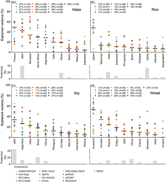
Figure 1. Explained variance of country-level yield anomaly for top ten producer countries for (a) maize, (b) rice, (c) soy, and (d) wheat. Explained variance (R2) refers to simulated yield from the respective model and observed yield from FAO data. For each model, the run with the highest mean explained variance across the top ten producer countries is shown. Black line is the median across the shown model runs for each country. Grey bars illustrate the average share in global production per country. The legend in each panel shows mean explained variance across top ten producer countries and sample size (details tables S3–S6 and figures S2–S5).
Download figure:
Standard image High-resolution imageFor each crop, individual models can explain more than 50% of the yield anomaly for several main crop producer countries (figure 1). Specifically, for the USA, France, Argentina, South Africa, and Romania for maize; Japan for rice; USA, Argentina, and India for soy; and Australia, Canada, and Turkey for wheat. There was no single model that outperformed all others, and there was typically a large variation between individual models (figure 1 and tables S3–S6) but also between different runs of an individual model (figures S2–S5). In addition, no climate forcing dataset was superior to others, nor were 'fullharm' runs better than 'default' runs (figures S2–S5).
3.2. Impact of extreme events on yield
The observed mean relative yield decline calculated from FAO data under droughts was 4.3% for maize, 1.3% for rice, 3.4% for soy and 6.7% for wheat. Relative yield decline induced by heatwaves was 8.2% for maize, 2.2% for soy and 4.5% for wheat. For rice, FAO data showed no signal for the year of the heatwave event (figure S1), which is in line with Lesk et al (2016). In contrast, there was an event signal for drought events (figures S1). We thus excluded heatwave events from our analysis for rice.
Across all crops and both event types, the majority of models detected the event signal, except for the impact of heatwaves on wheat and droughts on rice. Models typically either reproduced observed losses or underestimated yield decline, and underestimation was often strong. While yield is over- or underestimated in non-extreme years, yield decline is rarely overestimated (except CGMS-WOFOST, and several models for soy), suggesting that models systematically detect the event signal of extreme years. The mean percent bias across all models was negative across all crops and event types, which confirms the underestimation of yield decline for extreme years. Specifically, multi-model mean percent bias was −1.74 for maize and drought, −3.19 for maize and heat, −3.20 for wheat and drought, −2.66 for wheat and heat, −0.44 for rice and drought, −0.62 for soy and drought, and −0.56 for soy and heat.
For maize and drought, 12 of the 13 models detected the event signal (figure 2). Especially the simulations by PEPIC and CGMS-WOFOST were close to the observed impact. PEPIC showed a high agreement between observed and simulated yield declines for both observational climate datasets that were used to run the model, suggesting that good performance is not random. In contrast, for the second type of composite, all models detected the event signal and simulated the drought impact close to the observed estimate (figure S7). For maize and heatwaves, eleven models detected the signal, and five models were close to the observed impact (EPIC-Boku, PEPIC, CGMS-WOFOST, GEPIC, pAPSIM, figure 3). For wheat, all models detected the drought signal (especially, ORCHIDEE-Crop and EPIC-Boku), but most underestimated the yield impact, some strongly (figure 4). Only CGMS-WOFOST slightly (−9.2% versus −7.9%) overestimated the impact. Some models performed better for the absolute difference than for the relative ones (e.g. LPJmL, ORCHIDEE-Crop and PDSSAT, figure S25). For wheat and heatwaves, six models detected the event signal (e.g. CLM-Crop, PEPIC, figure 5). Performance was not better for the absolute deviations than for the relative ones considered here (figure S28).
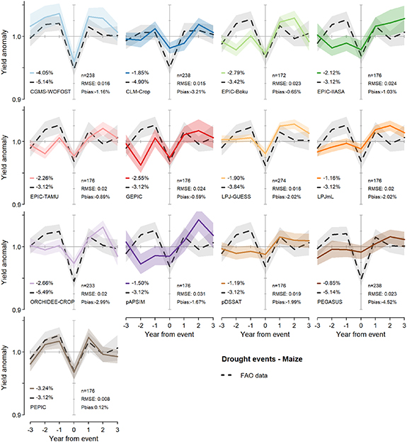
Figure 2. Mean impact of drought events on maize yields. Composites are based on seven year window of country-level relative yield deviations from long-term means. Results are shown for the best run for each model (coloured line) compared to observed impact (black line). Shaded area is the standard error. All model runs in figure S6. Legends detail mean event impact of model simulation and FAO data, number of events included, root mean square error (RMSE, unitless), and percent bias (Pbias).
Download figure:
Standard image High-resolution image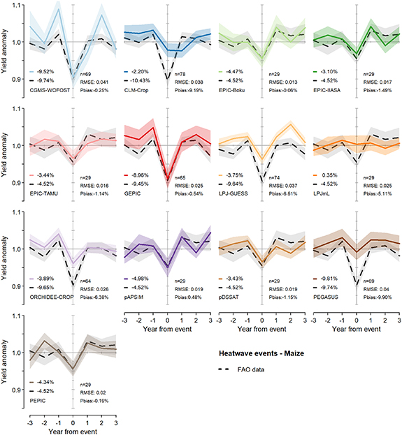
Figure 3. Mean impact of heatwave events on maize yield. Composites are based on 7-year window of country-level relative yield deviations from long-term mean. Results are shown for the best run for each model (coloured line) compared to observed impact (black line). Shaded area is the standard error. All model runs in figure S9. Legends detail mean event impact of model simulation and FAO data, number of events included and root mean square error (RMSE, unitless), and percent bias (Pbias).
Download figure:
Standard image High-resolution image
Figure 4. Mean impact of drought events on wheat yield. Composites are based on 7-year window of country-level relative yield deviations from long-term mean. Results are shown for the best run for each model (coloured line) compared to observed impact (black line). Shaded area is the standard error. All model runs in figure S24. Legends detail mean event impact of model simulation and FAO data, number of events included and root mean square error (RMSE, unitless), and percent bias (Pbias).
Download figure:
Standard image High-resolution image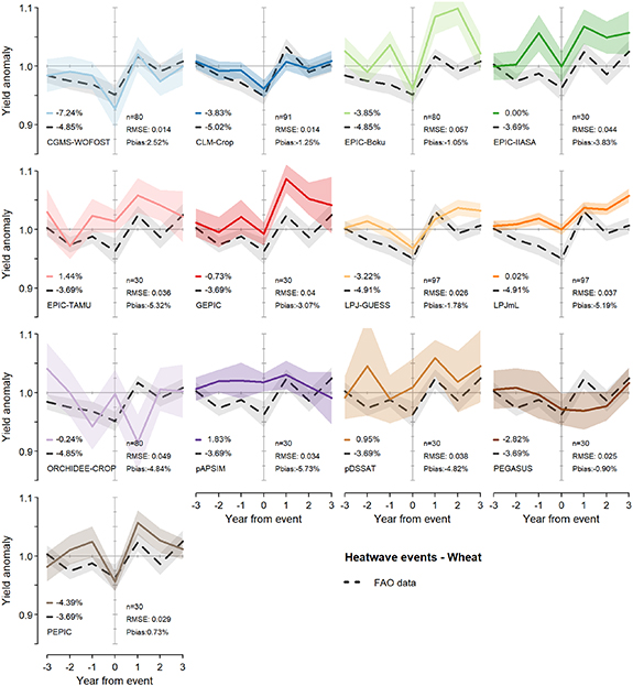
Figure 5. Mean impact of heatwave events on wheat yield. Composites are based on 7-year window of country-level relative yield deviations from long-term mean. Results are shown for the best run for each model (coloured line) compared to observed impact (black line). Shaded area is the standard error. All model runs in figure S27. Legends detail mean event impact of model simulation and FAO data, number of events included and root mean square error (RMSE, unitless), and percent bias (Pbias).
Download figure:
Standard image High-resolution imageFor rice and drought, five models out of ten detected the event signal (e.g. GEPIC, LPJmL, figure S12). For soy and drought, ten of twelve models detected the event signal, with most of these models simulating the impact close to the observed impact (e.g. GEPIC, pAPSIM, pDSSAT, LPJmL, figure S16). Four models overestimated the yield impact. For the second composite, some models performed better (e.g. EPIC-IIASA, PEPIC, ORCHIDEE-Crop). For soy and heatwaves, nine of the twelve models detected the event signal (e.g. EPIC-Boku, LPJ-GUESS, GEPIC, PEPIC, figure S20). CGMS-WOFOST overestimated the impact.
Comparing model performance, PEPIC reproduced observed maize (drought and heatwave) and wheat yield well (drought, but not heatwave). In contrast, there were models that performed well for one but not the other. For example, LPJmL reproduced yield decline close to observed decline for wheat and drought, but not for heatwave; and EPIC-Boku reproduced yield decline well for maize and heatwave, but not for wheat and heatwave. When comparing runs of individual models, climate forcing datasets had a stronger effect than harmonization settings, meaning default versus fullharm runs (e.g. GEPIC and pDSSAT in figure S6). As differences between default and fullharm settings can differ between models and they could be very similar depending on the model specifications, this finding does not allow for further inferences.
When comparing model performance for country-level yield anomaly with extreme event impact on yield (figure 6), PEPIC and pDSSAT performed well across all analyses for maize. GEPIC, which had the highest R2 for country-level yield anomaly for maize, had moderate RMSE values for drought and heatwave impact on yield, but the yield decline estimated for the year of the event was close to the observed impact (figures 2 and 3).
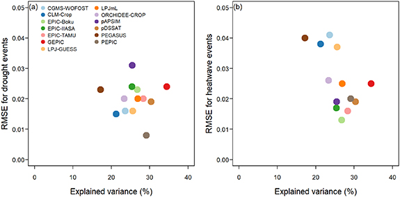
Figure 6. Comparing model performance for reproduction of variability across top 10 producer countries (mean explained variance) with performance for (a) drought and (b) heatwave impact on maize. RMSE is the root mean square error and is unitless.
Download figure:
Standard image High-resolution image3.3. Growing season
We found that model runs with a higher growing season mean EDD, tended to better reproduce the observed yield loss induced by heatwaves, especially for maize and wheat (figure 7). However, there was a large variation between runs of the same model and between different models. For drought events, we did not find a relationship between model performance and precipitation during simulated growing seasons (figure 8). When further investigating why there was no relationship, we found a large variation in performance between individual drought events. While for certain drought events the relationship between model performance and precipitation was as expected, for others there was a large difference between modelled and observed yield impact, even though there was low precipitation, or the other way around (small difference in yield impact and high precipitation) (figure S30). The latter was, for example, the case when there was large spatial variation in precipitation with flooding in some parts of the country and drought in others (e.g. drought in Ecuador 1997).
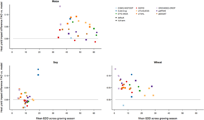
Figure 7. Comparison of overlap between simulated growing season with heatwave events (measured as extreme degree days (EDD) across growing season, higher EDD means stronger overlap with heatwaves) and model performance (measured as difference between yield decline caused by heatwaves from FAO data versus model simulations).
Download figure:
Standard image High-resolution image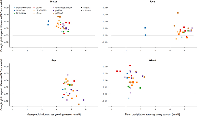
Figure 8. Comparison of overlap between simulated growing season with drought events (measured as mean precipitation across growing season, lower precipitation means stronger overlap with drought event) and model performance (measured as difference between yield decline caused by droughts from FAO data versus model simulations).
Download figure:
Standard image High-resolution image
4. Discussion
4.1. Inter-annual variability in national yields
Comparing simulations across 13 models, some models explained more than 50% of the yield variability for several of the major crop producer countries, for example, for five of the ten top maize producers (figure 1). There was a large variation between individual models and between different runs of the same model on how well yield anomalies were reproduced, which is in line with previous intercomparisons of GGCMs forced by different climate datasets (Frieler et al 2017, Müller et al 2017). Models performed particularly well for countries such as Romania and France for maize yield, Australia and Canada for wheat, Japan for rice (Frieler et al 2017, Jägermeyr and Frieler 2018, this study). In addition, there are model runs included in this study that performed better for maize yield in China (second largest maize producer), soy yield in USA (largest soy producer) and India, and rice yield in China (largest rice producer), Thailand and Brazil.
Yield variability is driven not only by weather, but also by management decisions and reporting errors, that cannot be captured by the GGCMs. GGCMs evaluated here explained variances of observed de-trended yields of around 30% for maize and less than 20% for rice, with likely too low values for rice due to underperformance of the models. Ray et al (2015) found that around one third of global crop yield variability is caused by climate variability on a sub-national scale. In addition, they found that climate variability had a stronger impact on countries with high-input agriculture, which is reflected in GGCMs that performed better for these countries than for countries with low-input agriculture (figure 1).
4.2. Impact of extreme events on yield
Overall, GGCMs were able to simulate the impact of droughts and heatwaves on crop yield. While the majority of models detected the event signal, fewer models estimated the magnitude of yield decline close to the observed decline. Those models performed similarly well as variations of the LPJmL model evaluated in an earlier study (Jägermeyr and Frieler 2018). However, there was not a single model (or set of models) that outperformed all others across the different crops and event types. Similarly to earlier findings pertaining to the European heatwave in 2003 (Schewe et al 2019), the majority of GGCMs that detected the event signal underestimated the magnitude of yield decline. One possible explanation is that model simulations do not necessarily lead to crop failures after severe weather but in many models, plants continue to grow when conditions become suitable again. In addition, models do not account for the influence of diseases and pests that have a stronger impact on stressed plants. In contrast, for soy, simulated yield impact was close to observed impact for the majority of models, with several overestimating yield decline. Models that explain year-to-year crop variability well also performed well for the impacts of heatwave events, with no clear relation for drought events (figure 6).
Compared to maize, model performance was worse for simulating the impact of heatwaves on wheat yield and the impact of drought on rice yields. For wheat, it is known that yield is sensitive to temperature stress (Zampieri et al 2017), and at the same time model uncertainty increases with higher temperatures (Asseng et al 2013). Another explanation might be a mismatch of simulated growing seasons, as we found that model runs for which the simulated growing season overlapped less with heatwaves performed worse (figure 7). For rice, yield is less strongly impacted by drought, with an estimated yield decline from observed FAO data at only 1.3%. This is likely due to rice being mostly grown under irrigated conditions. In addition, models seem to perform worse for rice in general, as shown in the first analysis on national yield variability, as median explained variance was below 20% for all major rice producer countries, except for Japan (figure 1).
By having two different composites, we were able to indirectly compare model performance in low versus high yield countries. For most crops and event types, both composites were very similar. However, for the impact of drought events on maize yield, models performed better in the second type of composite (figure S7 compared to figure 2), meaning when the yield decline was not weighted by overall yield. This could suggest that models do not adequately represent crop yield declines in countries with low yields, even though declines there can have detrimental impacts on food security (FAO 2018). Although global yield has grown during past decades, the impact of yield loss caused by extreme events continues to be of concern as high-yield countries are more strongly affected by weather induced yield shocks than countries with lower yields (Lesk et al 2016).
We also found that a model performing well for droughts did not necessarily perform well for simulating the impact of heatwaves, and vice versa (e.g. pAPSIM for maize, and ORCHIDEE-CROP for wheat). Even though droughts and heatwaves often co-occur, the ecological impact on plants differs (Brodribb et al 2020), and models differ in how they represent the processes of either or both. However, previous evaluations showed that GGCMs are able to reproduce the impact of high temperatures on yield (Schauberger et al 2017).
There were large differences between different runs of the same model in how well yield declines are reproduced (figures S6–S29). We found that the choice of climate forcing dataset and harmonization settings can have a strong impact on simulated yield, though no climate dataset nor harmonization setting was superior to others.
4.3. Limitations
Though being the most comprehensive database on national crop yield and production, data quality from the FAO database differs across countries (World Bank 2010). This introduces uncertainty in the analysis as low explained variance does not have to imply that model simulations are erroneous. A potential additional source of uncertainty are the extreme events chosen for this analysis. Extreme events are rare, which resulted in small sample sizes for heatwaves. When analysing the impact composites for the different time periods covered by model simulations, the calculation of the corresponding FAO data revealed that individual extreme events can have a strong impact on the multi-year average (see difference in grey line across panels in figure 2). In addition, extreme events can affect only part of a country and thus aggregation at the country level can introduce further uncertainty.
The impact of extreme events on yield is not only a response to the weather signal but also reflects which means farmers have available to buffer adverse conditions, for example, irrigation that can counteract the negative impact of high temperatures to a certain extent (Schauberger et al 2017, Vogel et al 2019). Temporal variations in adaptations are not accounted for in crop models, but could be integrated if, for example, data would be available on temporal changes of the proportion of irrigated land. In addition, yield is influenced by socio-economic factors that are not considered in GGCMs, such as plant diseases, insect pests, limited access to agricultural inputs such as fertilizers or pesticides, or limited access to farms during violent conflicts or epidemics (FAO 2018).
4.4. Conclusion
In general, GGCMs detect yield decline caused by droughts and heatwaves, but underestimate the magnitude of yield decline. This can imply that future projections of crop yield under climate change also underestimate the impact of extreme events. As the area exposed to extreme events is projected to increase (Lange et al 2020), the further advancement of GGCMs would be an important step in supporting evidence-based decision-making in light of ensuring future food security. Important model improvements include advancing the process representation and parameterization of the models, particularly with respect to heat stress and tissue damage under extreme temperatures, but improving model inputs is as important. Particularly a better global crop calendar product based on local observational data from various sources ideally with annual resolution would allow for a better growing season representation. However, crop yield anomalies are only partly driven by weather, and crop models cannot reproduce all the variation, as long as factors such as pests, economic and social issues are not considered. Thus, inter-sectorial modelling, i.e. combining crop models with models from other sectors, could be an important step towards adequately representing the impact of extreme events on crop production.
Acknowledgments
For their roles in producing, coordinating, and making available the ISIMIP input data and impact model output, we acknowledge the modelling groups (listed in table S1 of this paper), the ISIMIP sector coordinators and the ISIMIP cross-sectoral science team for the agricultural sector. This research has received funding from the German Federal Ministry of Education and Research (BMBF) under the research project ISIAccess (16QK05). This work was also supported by the Defense Advanced Research Project Agency under the World Modelers programme (Grant No. W911NF1910013). J J was supported by the NASA GISS Climate Impacts Group and the Open Philanthropy Project.
Data availability statement
The data that support the findings of this study are openly available at the following URL/DOI: https://data.isimip.org/.