Significant Improvement in Soil Organic Carbon Estimation Using Data-Driven Machine Learning Based on Habitat Patches

Abstract

Soil organic carbon (SOC) is generally thought to act as a carbon sink; however, in areas with high spatial heterogeneity, using a single model to estimate the SOC of the whole study area will greatly reduce the simulation accuracy. The earth surface unit division is important to consider in building different models. Here, we divided the research area into different habitat patches using partitioning around a medoids clustering (PAM) algorithm; then, we built an SOC simulation model using machine learning algorithms. The results showed that three habitat patches were created. The simulation accuracy for Habitat Patch 1 (R² = 0.55; RMSE = 2.89) and Habitat Patch 3 (R² = 0.47; RMSE = 3.94) using the XGBoost model was higher than that for the whole study area (R² = 0.44; RMSE = 4.35); although the R² increased by 25% and 6.8%, the RMSE decreased by 33.6% and 9.4%, and the field sample points significantly declined by 70% and 74%. The R² of Habitat Patch 2 using the RF model increased by 17.1%, and the RMSE also decreased by 10.5%; however, the sample points significantly declined by 58%. Therefore, using different models for corresponding patches will significantly increase the SOC simulation accuracy over using one model for the whole study area. This will provide scientific guidance for SOC or soil property monitoring with low field survey costs and high simulation accuracy.

1. Introduction

As the most extensive carbon sink in the terrestrial environment, soil is a vital component of global carbon exchange [1,2]. The incorporation of soil organic carbon (SOC) is a crucial element in maintaining soil health and contributes significantly to improvements in the physicochemical properties of soil [3]. SOC represents between 50% and 80% of the carbon in the entire terrestrial ecosystem, surpassing three times that of vegetation and the atmosphere [4], and it affects the capacity of carbon sources and sinks in landscapes [5]. The traditional approach of conducting ground surveys and field sampling is time-consuming and costly, rendering them suitable only for small-scale monitoring [6]. It is therefore essential that the accurate prediction of SOC levels is performed using robust and economical methods [7,8]. At present, studies focus on using one single model to simulate the SOC in the whole study area. However, spatial heterogeneity can be very high in a complex subsurface, such as in the karst region of southwest China. For these complex regions, using a single model to simulate SOC will lead to a lower simulation accuracy. Therefore, a reasonable division of the whole study area into several sections and sub-regional modeling may improve the SOC estimation accuracy and decrease the field survey cost.

Few studies have divided the study area into different regions for SOC estimation. Recent studies have mapped SOC with digital soil mapping techniques in different land uses [9,10]. Coincidentally, clustering technology is the process of discovering and revealing the potential structures and patterns of datasets themselves. It can be used to divide the samples of the dataset into several disjoint clusters, so that each cluster corresponds to a potential type [11]. Among the many clustering methods, the well-known methods for implementing nonhierarchical clustering include K-means clustering and partitioning around medoids (PAM) [12]. The most central object in a cluster is chosen as its representative by the K-medoids algorithm, distinguishing itself from K-means clustering through its greater robustness to outliers. PAM, proposed in [12], has been widely recognized as the most robust and effective technique among the numerous techniques available for K-medoid clustering. Therefore, in this study, the PAM algorithm was used to carry out the division of study area, and the sub-regions were defined as habitat patches. In this study, we defined habitat patches as “The ecological environment characteristic space formed under the influence of similar natural and human factors, and the relative homogeneity of environmental factors within the patch, including the state and temporal variation characteristics of the elements.” This concept combines an overview of habitats and patches in ecology. Among these, “patches” usually refer to specific habitat types or characteristics within a geographic area, such as forest patches, wetland patches, etc., that represent a meaningful ecological entity [13]. “Habitat” usually refers to the environment in which a biological population or community exists and thrives in a specific geographic space, including both biotic and abiotic elements [14]. Then, the SOC content and spatial area were determined by digital soil mapping, proposed by [15], which has enabled the successful application of a growing number of machine learning algorithms to predict soil properties [16].

Among the machine learning algorithms, random forest (RF) [17] and extreme gradient boosting (XGBoost) [18] have been shown to be superior in the prediction of SOC content. The RF model is a nonlinear algorithm that relies on an ensemble decision tree. During the training process, the RF model possesses the ability to identify interaction among features. This unique approach avoids model autocorrelation and overfitting, thereby enhancing the reliability of the model’s predictions. Hence, it is the most prevalent and exceptionally precise technique in the domain of machine learning algorithms [19]. The XGBoost algorithm, known for its ability to accommodate complex nonlinear relationships and its excellent parallel processing capability, offers a promising solution to address the overfitting issue commonly encountered in machine learning models, especially with limited sample sizes collected from field experiments [20]. Moreover, various other machine algorithms, including support vector machine (SVM) [21], artificial neural network (ANN) [22], and convolutional neural network (CNN) [23], have also been employed to predict soil properties.

Accompanied by the explosion of spatiotemporal big data, multi-source data such as topography, climate, soil texture, and remote sensing images, are widely used for SOC content estimation [24]. Precipitation and temperature are key climatic factors that determine the content and spatial variation of SOC. On one hand, these two climatic factors directly influence plant growth processes and the net primary productivity of vegetation. On the other hand, the hydrothermal conditions of the climate largely shape the decomposition and accumulation dynamics of SOC. It is particularly noteworthy that the global warming trend has intensified the promoting effect of microbial activity on the rate of SOC decomposition [25]. The soil types mainly include paddy soil and acid purple soil. Soil type differences lead to differences in SOM content [26]. Application of remote sensing data introduces a significant improvement in the ability to predict the SOC content [27], due to its high spatial and spectrum resolution. In particular, optical satellite images have gained widespread usage in SOC prediction. For example, previous studies have predicted soil properties using reflectance bands and vegetation indices [28,29]. In addition, synthetic aperture radar (SAR) has been used for vegetation species mapping [30] and SOC content remote sensing inversion [31], relying on its ability to penetrate the surface, as it is unaffected by clouds and rain. The authors of [31] also proved that multitemporal SAR data can successfully predict soil properties by effectively capturing the intricate correlation between soil characteristics and vegetation growth.

We estimate the SOC in the karst trough area of southwest China in different habitat patches using multi-source data based on machine learning algorithm. The aims are (1) to explore the applicability of optical and SAR data in predicting the SOC content in karst areas and (2) to determine whether the estimation accuracy using different models in different clusters will be higher than that using one model for the whole study area.

2. Materials and Methods

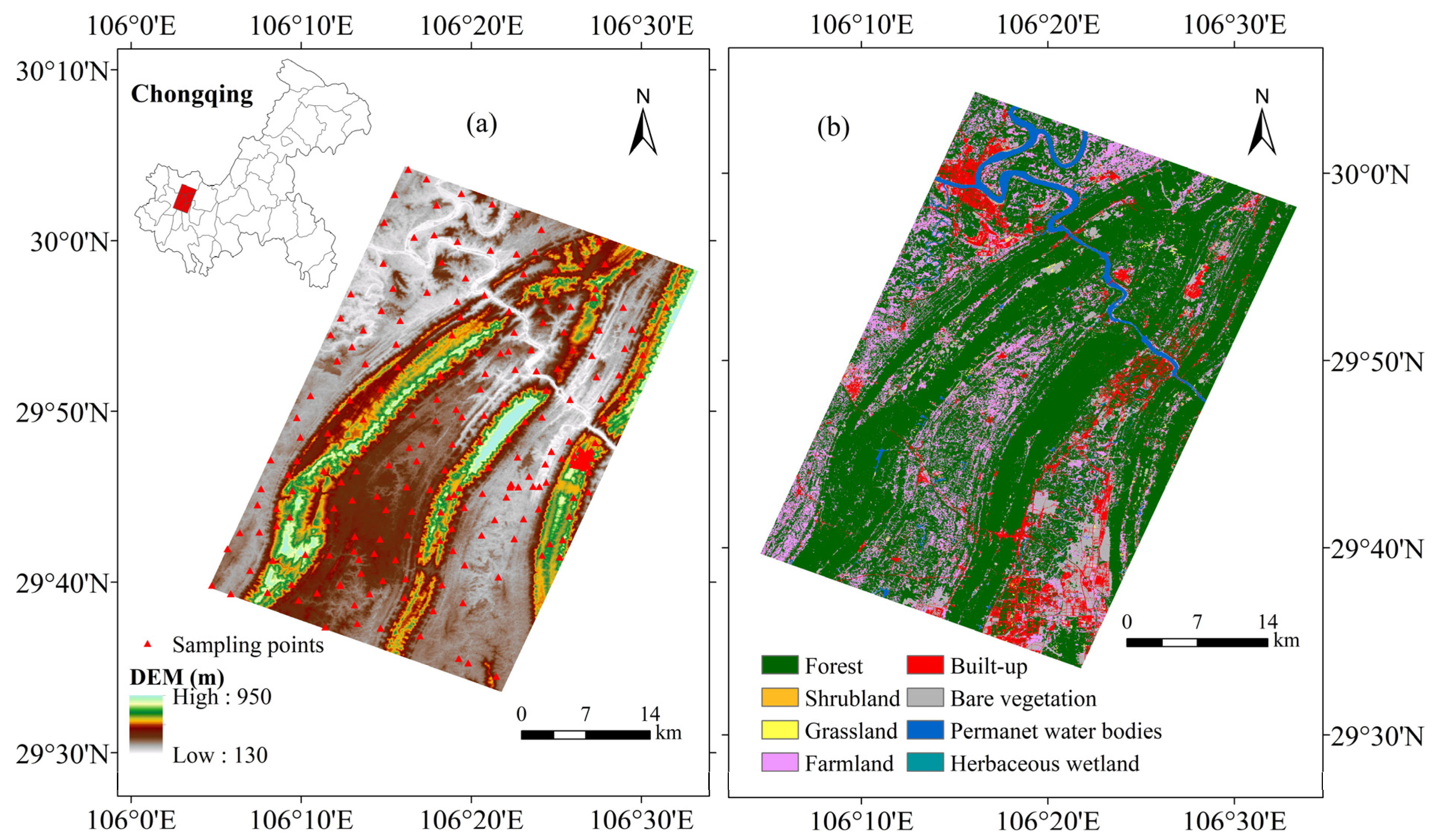
2.1. Study Area

The study area was in the northwestern region of Chongqing Province, which is in the southwest of China (Figure 1). The study area covers approximately 1200 km² and extends longitudinally from 106°4′ to 106°34′E and latitudinally from 29°31′ to 30°5′N. The terrain has an elevation range from 130 to 950 m. In the subtropical region, the climate is classified as humid monsoon, with prolonged periods of high temperatures during the summer and relatively mild and dry conditions during the winter. The mean annual temperature is 13.6 °C, while the estimated mean precipitation is 1600 mm. This study area is karst landform, with a high extent of urbanization and agricultural activity. The soil environment has basic characteristics such as thin soil layers, discontinuous distribution, and complex and diverse micro landforms. In addition, the impact of human activities on the land is prominent in the region, with severe soil erosion, as well as a significant loss of SOC, leading to serious ecological and environmental problems such as land desertification [32]. Therefore, the natural conditions and human impact on this region have led to a complex earth surface and high spatial heterogeneity. A previous study also proved that spatial heterogeneity was high in this area, and the representativeness of sampling sites was very important for remote sensing data validation [33].

2.2. Acquisition and Treatment of Data

All variables were used to identify driving factors and were converted to a 10 m spatial resolution grid using the nearest neighbor resampling method. For each soil sampling point, the pixel values associated with the variables were extracted based on these raster data.

2.2.1. Collection and Treatment of Soil Samples

In 2020 and 2021, a comprehensive soil-sampling survey was conducted within the study region, whereby topsoil samples (0–20 cm) were collected in 271 sample plots, which was carried out by employing a rigorous methodology. We used a five-point mixed sampling method within each sample plot and considered the spatial heterogeneity of the landform. To ensure accurate geolocation, a portable GPS system was employed to obtain the central grid coordinates associated with the collection of topsoil samples. Furthermore, to minimize soil cross-contamination and facilitate proper soil storage, each soil sample was carefully put into a fabric container to ensure proper handling and preservation of the samples collected. In the laboratory setting, the air-dried samples were subjected to grinding and sieving procedures, yielding particles with a size of ≤2 mm. Subsequently, the potassium dichromate heating method was used for SOC measurement [34].

2.2.2. Auxiliary Variables

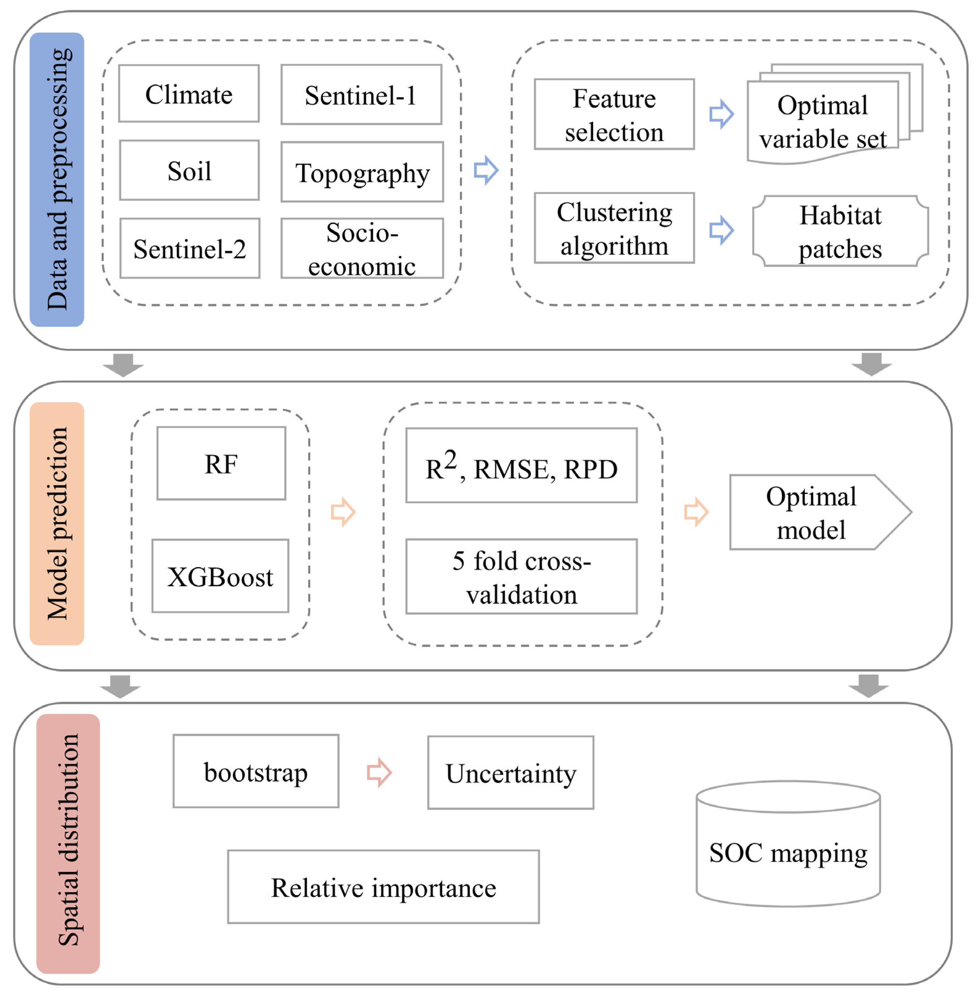
The auxiliary data included variables derived from remotely sensed images (27 variables from Sentinel-2A and Sentinel-1A), environmental data (10 variables), and three soil data types (sand content, silt content, and clay content). The acquisition dates were closely aligned with the timing parameters of the January 2020 and 2021 field data collection. We took the mean of the images as the input spectral reflectance value. Sentinel-2A data at 10m spatial resolution, derived from the Multispectral Instrument (MSI) L2A product, were pre-processed by the European Space Agency (ESA). This preprocessing included radiometric calibration and atmospheric correction to ensure that the acquired data accurately represented the surface reflectance information. The Sentinel images were downloaded from Google Earth Engine [35]. The employed spectral indices included the brightness index (BI), second brightness index (BI 2), color index (CI), clay index (CI 1), green–red vegetation index (GRVI), green normalized difference vegetation index (GNDVI), land surface water index (LSWI), second modified soil-adjusted vegetation index (MSAVI2), moisture stress index (MSI), normalized differences vegetation index (NDVI), redness index (RI), soil-adjusted total vegetation index (SATVI), soil-adjusted vegetation index (SAVI), transformed vegetation index (TVI), and vegetation (V) (

Table 1. Derived indicators from Sentinel-2A satellite images.

Index	Definition	Reference
BI	$\frac{\sqrt{\left(\rho Red\times \rho Red\right)+(\rho Green\times \rho Green)}}{2}$	[40]
BI2	$\frac{\sqrt{\left(\rho Red\times \rho Red\right)+\left(\rho Green\times \rho Green\right)+\left(\rho NIR\times \rho NIR\right)}}{3}$	[40]
CI	$\frac{\rho Red-\rho Green}{\rho Red+\rho Green}$
CI1	$\frac{SWIR1}{SWIR2}$	[41]
GRVI	$\frac{\rho Green-\rho Red}{\rho Green+\rho Red}$	[42]
GNDVI	$\frac{\rho NIR-\rho Green}{\rho NIR+\rho Green}$	[43]
LSWI	$\frac{\rho NIR-\rho SWIR1}{\rho NIR+\rho SWIR1}$	[44]
MSAVI2	$\frac{2\times \rho NIR+1-\sqrt{{(2\times \rho NIR+1)}^2-8\times (\rho NIR-\rho Red)}}{2}$	[45]
MSI	$\frac{\rho SWIR1}{\rho NIR}$
NDVI	$\frac{\rho NIR-\rho Red}{\rho NIR+\rho Red}$
RI	$\frac{\rho Red\times \rho Red}{\rho Green\times \rho Green\times \rho Green}$	[46]
SATVI	$\frac{\rho SWIR1-\rho Red}{\rho SWIR1+\rho Red+1}\times 2-\frac{\rho SWIR2}{2}$	[47]
SAVI	$\frac{(\rho NIR-\rho Red)\times 1.5}{\rho NIR-\rho Red+0.5}$	[48]
TVI	$\sqrt{\frac{\rho NIR-\rho Red}{\rho NIR+\rho Red}+0.5}\times 100$	[49]
V	$\frac{\rho NIR}{\rho Red}$	[50]

). Additionally, vertical–vertical (VV) and vertical–horizontal (VH) polarization data were used in this study. Land surface temperature (LST) was obtained from [36] (https://15203878955lz.users.earthengine.app/view/psc-app, accessed on 15 December 2023). The calculation of five topographic variables was derived from the Advanced Land Observing Satellite (ALOS) Digital Elevation Model (DEM) [37] at 12.5 m spatial resolution, including elevation, terrain undulation, slope, aspect, and topographic wetness index (TWI). The mean annual temperature and precipitation data at 1 km spatial resolution for the study area were obtained from the Resources and Environmental Science and Data Center of the Chinese Academy of Sciences (RESDC) (http://www.resdc.cn, accessed on 15 December 2023). Population density data were provided by the Socioeconomic Data and Applications Center (https://sedac.ciesin.columbia.edu/data/set/gpw-v4-population-density-rev11, accessed on 15 December 2023). Soil factors at 1 km spatial resolution were obtained from Soil Sub Center, National Earth System Science Data Center, National Science & Technology Infrastructure [38,39] (http://soil.geodata.cn, accessed on 15 December 2023).

2.3. Methods

To construct a highly accurate and regionally applicable prediction model for SOC content, we used the PAM algorithm to partition the study area into three distinct regions. Following this partitioning, the combination and selection of auxiliary variables was optimized for each section using a genetic algorithm (GA). Subsequently, predictive models of SOC content were created using the RF and XGBoost models. Finally, through the comparison of predicted outcomes from different regions, we achieved a digital map of the SOC content.

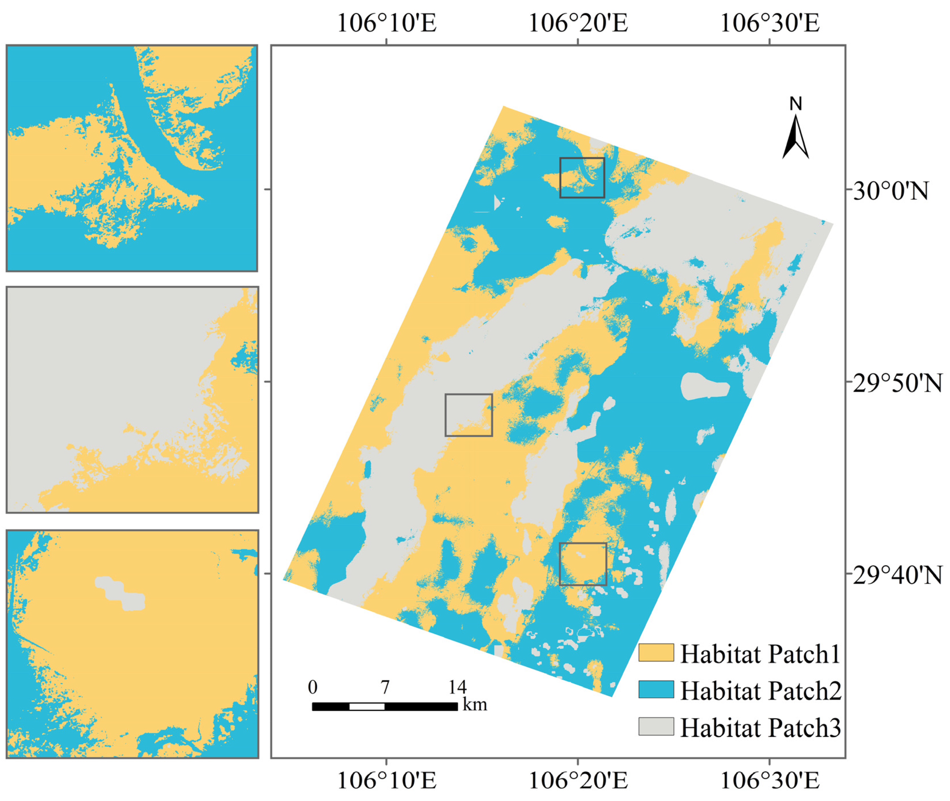
2.3.1. Cluster Algorithm

The PAM algorithm has been widely used in data clustering due to its ability to effectively group data points based on pairwise similarity values. Through an iterative learning process that exploits the similarity of the values among every pair of data objects, the algorithm optimizes the clustering of data objects by maximizing the aggregate similarity values with each cluster. As a result, the PAM algorithm can group data objects with similarity values equal to or less than a specified threshold into a single cluster. The cluster package in the R software was used for the execution of the PAM algorithm.

2.3.2. Feature Selection Method

The GA, originally proposed by Holland [51], is a metaheuristic approach that simulates biological evolution to find the best answers to an issue. As a heuristic search algorithm, the GA provides the optimal value for a given function, as demonstrated by Welikala et al. [52]. In the context of feature selection, the GA uses an initial population of individuals that are binary-coded to indicate whether a feature is selected (1) or not (0). These individuals represent different subsets of ancillary data and undergo a selection process to identify the most relevant features [33].

The proposed algorithm involves a sequence of three basic genetic operations, namely, selection, crossover and mutation, which are performed iteratively until a predetermined termination criterion is met. The selection operation is performed to identify the two most competent individuals based on their ability to minimize the root mean squared error (RMSE). The crossover operation is then applied to generate new solutions by recombining genetic information from two parent individuals, potentially leading to better performing offspring. In addition, the mutation operator is used to introduce genetic diversity by changing a limited subset of individuals. Until a specific termination criterion is met, the iterative mechanism of selecting, crossing over, and mutating continues [52]. Crucially, to facilitate estimating the RMSE by fitting a random forest model, the assignment of a fitness score to each member of the population becomes imperative with the establishment of each new cohort. In this study, the caret package in the R software was used to run the GA with five-fold cross-validation and 50 iterations with the goal of determining the smallest set of auxiliary variables that are significant for modeling SOC [53]. A population size of 50, a crossover rate of 0.8, and a mutation rate of 0.002 were used in the present study.

2.3.3. Prediction Models

As an ensemble-learning approach, RF leverages the construction of multiple decision trees, the outputs of which are combined to estimate the classification and regression. The RF methodology relies on the use of random binary trees constructed using bootstrapping techniques on a subset of observations. The model is developed by using a randomized subset of the original dataset for training purposes. The selected subset is used to create a representative sample of the original data, and through this process, the model is developed [54]. The use of RF has the notable advantage that the data used have properties of randomness and diversity. These characteristics produce results that are more accurate than those obtained from individual components [55]. In the context of tree induction, randomness can be achieved by changing the predictors, while replacement sampling can create diversity. The number of trees (ntree) was 600.

The XGBoost technique was first introduced by Chen and Guestrin [56], who presented a novel methodology to enhance the performance of gradient boosting through the optimization of the loss function and regularization of model complexity. It is an approach that focuses on regression trees and K-classification methods to increase the effectiveness of gradient boosting machines [57]. The basic concept of the proposed approach is to augment a “strong” learner by using supplemental training strategies from a group of “weak” learners, also known as boosting. The XGBoost technique is designed to increase computational efficiency while mitigating instances of overestimation. This is achieved by streamlining the objective functions and optimizing the computational speed by integrating estimation and adaptation terms. In addition, during the training process of the XGBoost method, the functions undergo simultaneous computations automatically. The type of model, learning rate, and depth of tree were gbtree, 0.4, and 7, respectively. In this study, a grid-search strategy was used to fine-tune all parameters using the caret package in the R software [58].

2.3.4. Evaluation of Prediction Accuracy

In this study, the evaluation of model performance and its ability to generalize effectively was performed using the five-fold cross-validation approach. Model performance was evaluated by calculating key evaluation metrics, including the coefficient of determination (R²), RMSE, and residual prediction deviation (RPD). The dataset was divided into five subgroups of approximately equal size. In each training process, 80% of the dataset was allocated for training purposes, while the remaining 20% was reserved for verification purposes. The cross-validation process was repeated five times, ultimately ensuring that each subset was used once for validation. The R², RMSE, and RPD values for each validation subset were computed. The aggregated performance of the model was determined by calculating the average of the R², RMSE, and RPD values derived from the five replicate runs. The R² value, which ranges from 0 to 1, indicates how well the independent predictors can explain the variation in the response variable. The RMSE serves as a measure of the prediction accuracy of the model. The RPD metric is used as an indicator of model quality, whereby 1.0 < RPD < 1.4 indicates a poor model; 1.4 < RPD < 1.8 indicates a fair model; 1.8 < RPD < 2.0 indicates a good model, where quantitative predictions are possible; 2.0 < RPD < 2.5 indicates a very good quantitative model; and RPD > 2.5 indicates an excellent model [59]. A full explanation of the equations is provided as follows:

$$\mathrm{R}\mathrm{M}\mathrm{S}\mathrm{E}=\sqrt{\frac{1}{\mathrm{n}}\sum _{\mathrm{i}=1}^{\mathrm{n}}{({\mathrm{P}}_{\mathrm{i}}-{\mathrm{M}}_{\mathrm{i}})}^2}$$

(1)

$${\mathrm{R}}^2={\left(\frac{\sum _{\mathrm{i}=1}^{\mathrm{n}}({\mathrm{M}}_{\mathrm{i}}-\overline{\mathrm{M}})({\mathrm{P}}_{\mathrm{i}}-\overline{\mathrm{P}})}{\sqrt{\sum _{\mathrm{i}=1}^{\mathrm{n}}{({\mathrm{M}}_{\mathrm{i}}-\overline{\mathrm{M}})}^2}\sqrt{\sum _{\mathrm{i}=1}^{\mathrm{n}}{({\mathrm{P}}_{\mathrm{i}}-\overline{\mathrm{P}})}^2}}\right)}^2$$

(2)

$$\mathrm{R}\mathrm{P}\mathrm{D}=\frac{{\mathrm{S}\mathrm{D}}_{\mathrm{M}}}{\mathrm{R}\mathrm{M}\mathrm{S}\mathrm{E}}$$

(3)

where M_i and P_i are the measured and predicted SOC content (g·kg ⁻¹), $\overline{M}$ and $\overline{P}$ indicate the average of the measured and predicted SOC content (g·kg ⁻¹), n represents the number of soil-sampling points, and SD_M denotes the standard deviation of the measured SOC content.

2.3.5. Uncertainty Analyses

The mix of uncertainties resulting from the model parameters, model inputs, and model structure contribute to the overall level of uncertainty in the modeling process [60]. When mapping is performed, the uncertainties should be considered in predicting soil properties based on this information [61]. To measure the uncertainty in predicting soil properties, a bootstrapping method was used in this study [62]. The full dataset was arbitrarily divided into two portions for each iteration of the bootstrap uncertainty analysis, with 70% going to training and 30% to validation. The best model was run 50 times using this technique, resulting in 50 prediction maps. Based on these prediction maps, the mean of the predicted values for each pixel was calculated as the final prediction map, while the standard deviation of the predicted values for each pixel was used as the uncertainty. The workflow of the current study is presented in Figure 2.

3. Results

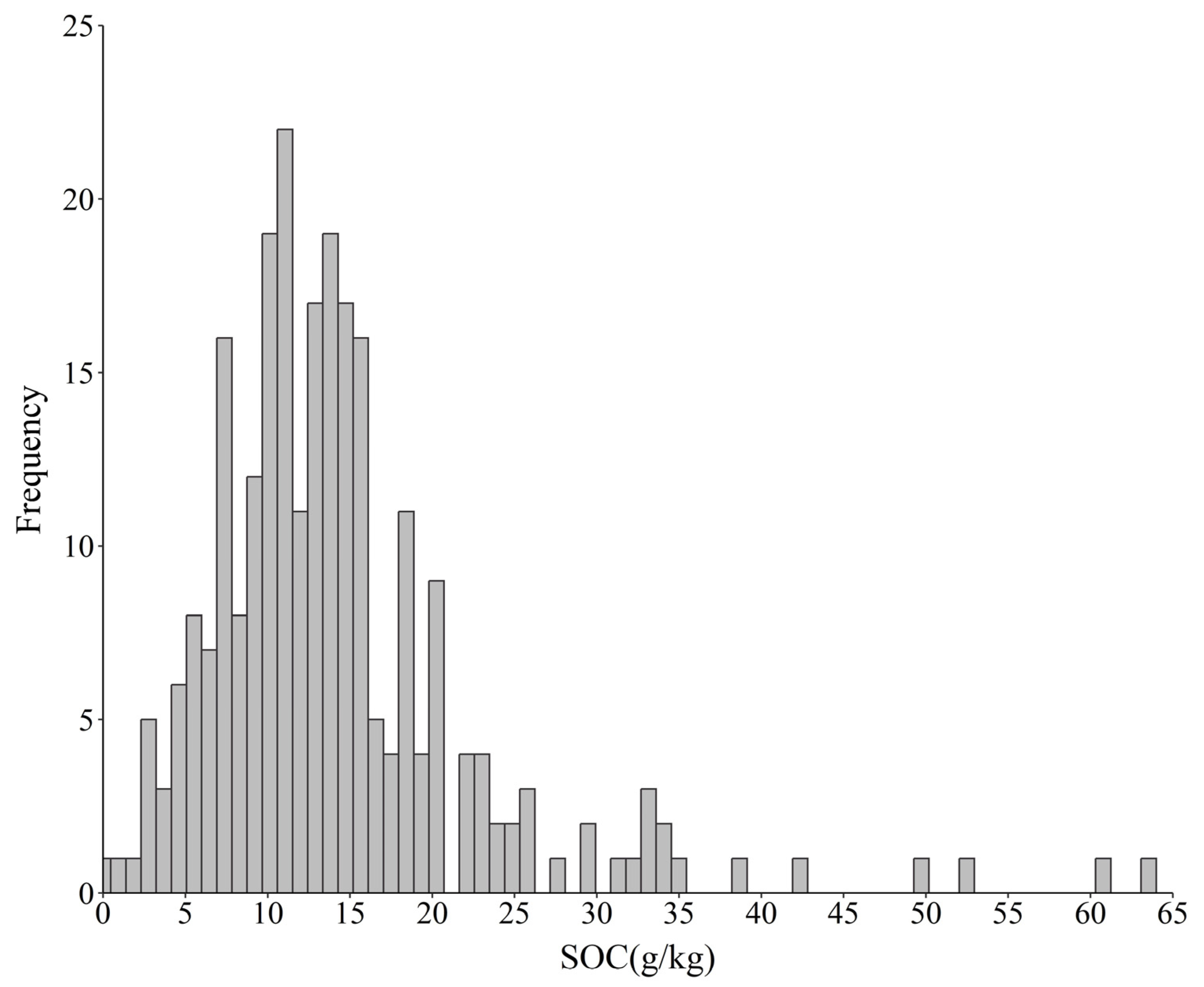
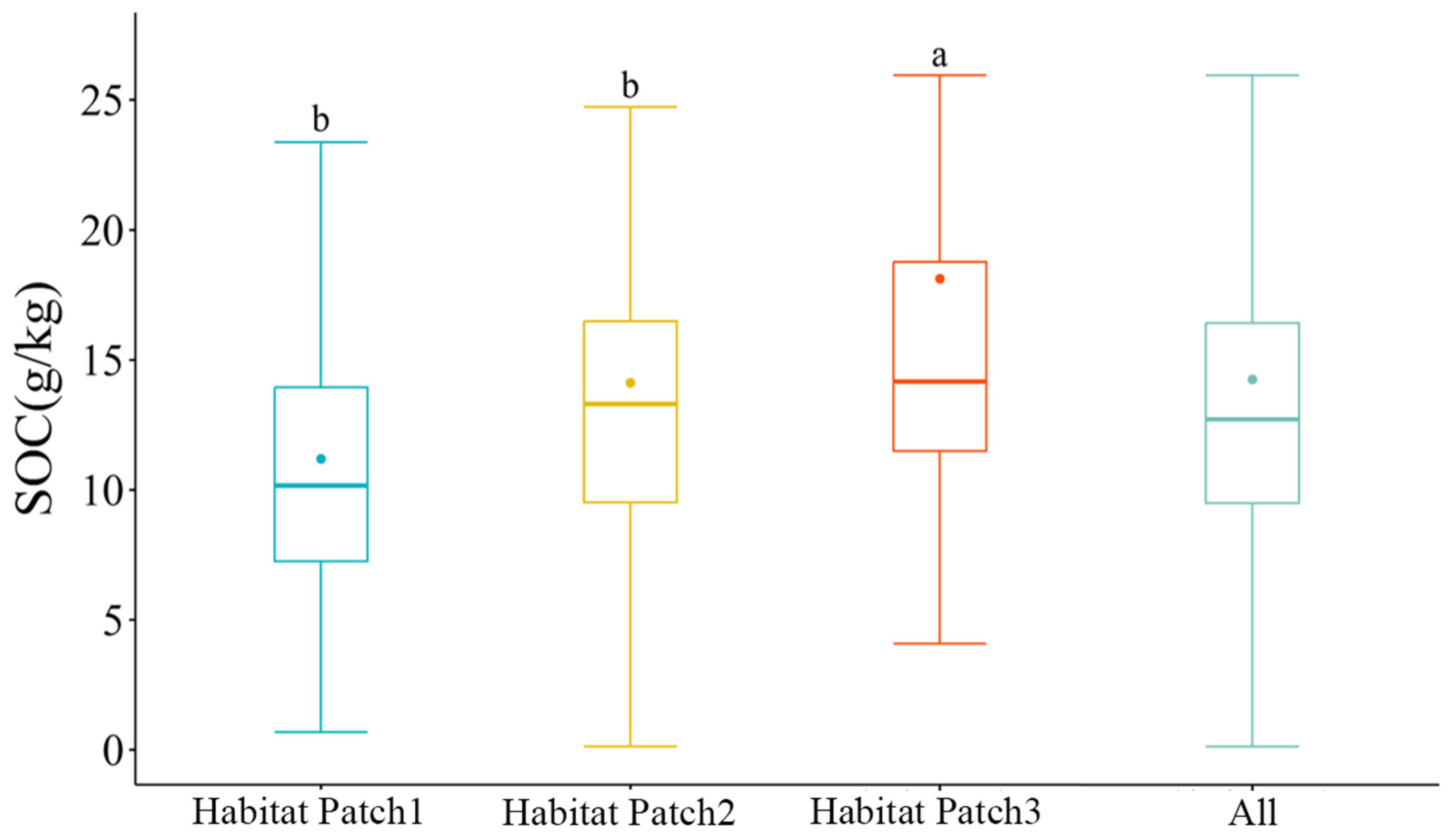
3.1. Descriptive Statistics of the SOC Content

The total SOC content varied widely from 0.12 to 63.66 g·kg ⁻¹ (Figure 3). The mean value of the SOC content was determined to be 14.25 g·kg ⁻¹, while the standard deviation and coefficient of variation were estimated to be 8.79 g·kg ⁻¹ and 61.68%, respectively (

Table 2. Statistical description of the SOC content in the overall study area and three habitat patches.

Sample Type	Sample Number	Minimum (g·kg −1)	Maximum (g·kg −1)	Average (g·kg −1)	Standard Deviation (g·kg −1)	Coefficient of Variation (%)
Overall	254	0.12	63.66	14.25	8.79	61.68
Habitat Patch 1	80	0.67	34.27	11.19	5.91	52.81
Habitat Patch 2	107	0.12	50.06	14.11	7.59	53.79
Habitat Patch 3	67	4.07	63.66	18.11	11.63	64.22

). The majority of SOC content measurements typically fell within a range of 5 to 20 g·kg ⁻¹, with a comparatively smaller proportion of values exceeding 40 g·kg ⁻¹. For Habitat Patch 1 and Habitat Patch 2, the mean value, standard deviation, and coefficients of variation all showed a decreasing trend. For Habitat Patch 3, the three indicators increased. The results indicated a remarkable degree of spatial variability in SOC content, as evidenced by the relatively high values of standard deviation and coefficient of variation. According to the results of the least significant difference analysis, the difference in SOC content between Habitat Patch 1 and the average SOC content of Habitat Patch 2 is not significant, but the difference in SOC content between Habitat Patch 3 and the average SOC content is significant (p < 0.05) (Figure 4).

3.2. Cluster Analysis and Feature Selection of Variables

The input variables of the PAM algorithm included NDVI, LST, terrain attributes (DEM), climatic data (e.g., precipitation and temperature), socioeconomic data (density of population), and soil data (e.g., content of sand, silt, and clay). The study area was divided into three sections using the PAM algorithm (Figure 5). Habitat Patch 1 has high arable land cover and medium elevation, Habitat Patch 2 has high urban cover and low elevation, and Habitat Patch 3 has dense forest cover and high elevation.

Based on the clustering results, the GA was applied as a feature selection method for each of the categories in the study area. A thorough process of trial and error was used to determine the characteristics of the GA model. The optimal values found were a population size of 60, a crossover probability of 0.8, and a mutation probability of 0.2. In running the GA model, a comprehensive set of 40 variables was evaluated, from which a subset of 14 variables were determined to be the most salient predictors in Habitat Patch 1, namely, temperature, population density, precipitation, GNDVI, CI1, V, slope, topographic relief, aspect, silt, clay, VV, VH, and band 11 of Sentinel-2A. Twenty-one variables were selected as the most significant set in Habitat Patch 2, namely, precipitation, population density, DEM, CI, GNDVI, CI1, LSWI, MSAVI2, RI, SATVI, SAVI, topographic relief, aspect, TWI, silt, clay, VV, VH, and bands 2, 3, and 12 of Sentinel-2A. Thirteen variables were selected as the best set of variables in Habitat Patch 3: temperature, LST, NDVI, DEM, BI, CI1, RI, SATVI, slope, and bands 4, 8, 9, and 11 of Sentinel-2A.

3.3. Simulation Accuracy of the Predictive Models

Table 3. Mean fit values of model performance for RF and XGBoost predictions of SOC.

Sample Type	Sample Numbers	Models	RMSE	R2	RPD
Habitat Patch 1	80	RF	3.69	0.23	1.07
		XGBoost	2.89	0.55	1.48
Habitat Patch 2	107	RF	4	0.41	1.21
		XGBoost	3.95	0.35	1.14
Habitat Patch 3	67	RF	5.98	0.36	1.06
		XGBoost	3.94	0.47	1.16
All	254	RF	4.47	0.34	1.16
		XGBoost	4.35	0.44	1.32

shows the results of using the RF and XGBoost models to predict SOC content based on five-fold cross validation. For Habitat Patch 1, the XGBoost model obtained the highest prediction accuracy, having the lowest RMSE (2.89) value and the highest R² (0.55) and RPD (1.48) values. For Habitat Patch 2, the RF model had the best performance with the highest R² (0.41) and RPD (1.21) values. For Habitat Patch 3, the XGBoost model showed the best prediction ability (R² = 0.47, RMSE = 3.94). The prediction accuracy of the SOC content based on the best model in Habitat Patch 1 and Habitat Patch 3 was higher than the prediction accuracy of the overall regional modeling. In Habitat Patch 2, the RF showed an increase in model performance, while the XGBoost showed a decrease in model performance. Based on the above analysis of accuracy comparison, XGBoost was used as the simulation model for Habitat Patch 1 and Habitat Patch 3, while RF was selected for Habitat Patch 2.

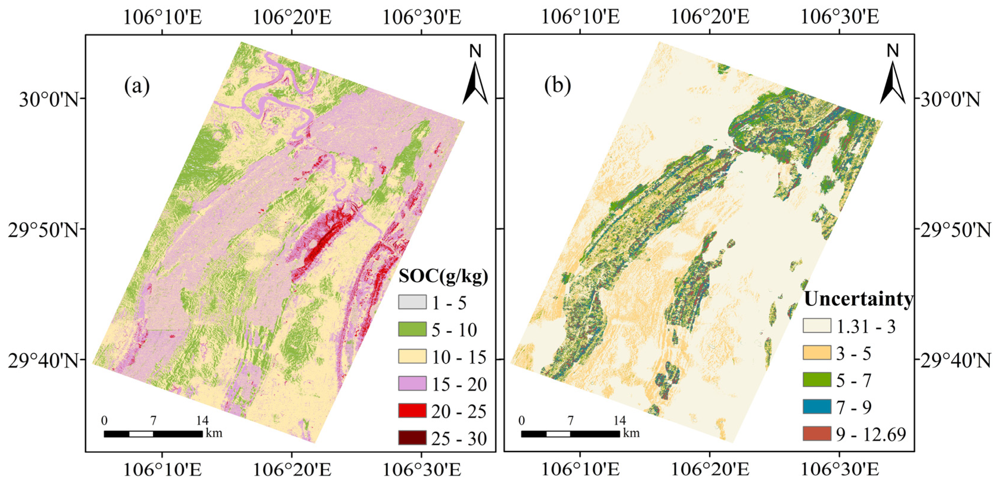
3.4. Spatial Distribution and Uncertainty of SOC Content

The spatial variation in SOC content and uncertainty was mapped using the RF (in Habitat Patch 2) and XGBoost algorithms (in Habitat Patch 1 and Habitat Patch 3) (Figure 6). With an average of 13.25 g·kg ⁻¹, the predicted values of the SOC content ranged from 1.88 to 30.00 g·kg ⁻¹. The predicted SOC variation was less than the measured SOC variation, confirming the inadequacy of the prediction map and model in estimating the maximum and minimum values of SOC. This finding was consistent with previous SOC prediction studies and highlighted the need for improved prediction models to accurately determine SOC concentrations [25,63,64]. Most of the predicted SOC values were between 10 and 20 g·kg ⁻¹, consistent with the range of most measured SOC values.

According to the uncertainty map, the uncertainty showed an increasing trend in Habitat Patch 1, Habitat Patch 2, and Habitat Patch 3. The highest uncertainty was in the Habitat Patch 3 area, with the highest spatial variation, while the lowest uncertainty was observed in the Habitat Patch 1 area. The largest uncertainties were mainly located in regions with lower predicted SOC levels.

In this study, there was a similar spatial pattern between elevation and SOC content, indicating that elevation and terrain characteristics significantly influence the spatial variability of the SOC content. A remarkable trend in the distribution of SOC content was discovered by this study, with the topographically elevated area in the eastern part of the study area showing a predominance of elevated SOC concentrations, while the lower elevation region in the west had predominantly lower SOC content. At higher elevations, characterized by colder temperatures, favorable light conditions and longer daylight hours promote photosynthesis in plants, thereby reducing the rate of SOC decomposition and increasing its input [65,66].

4. Discussion

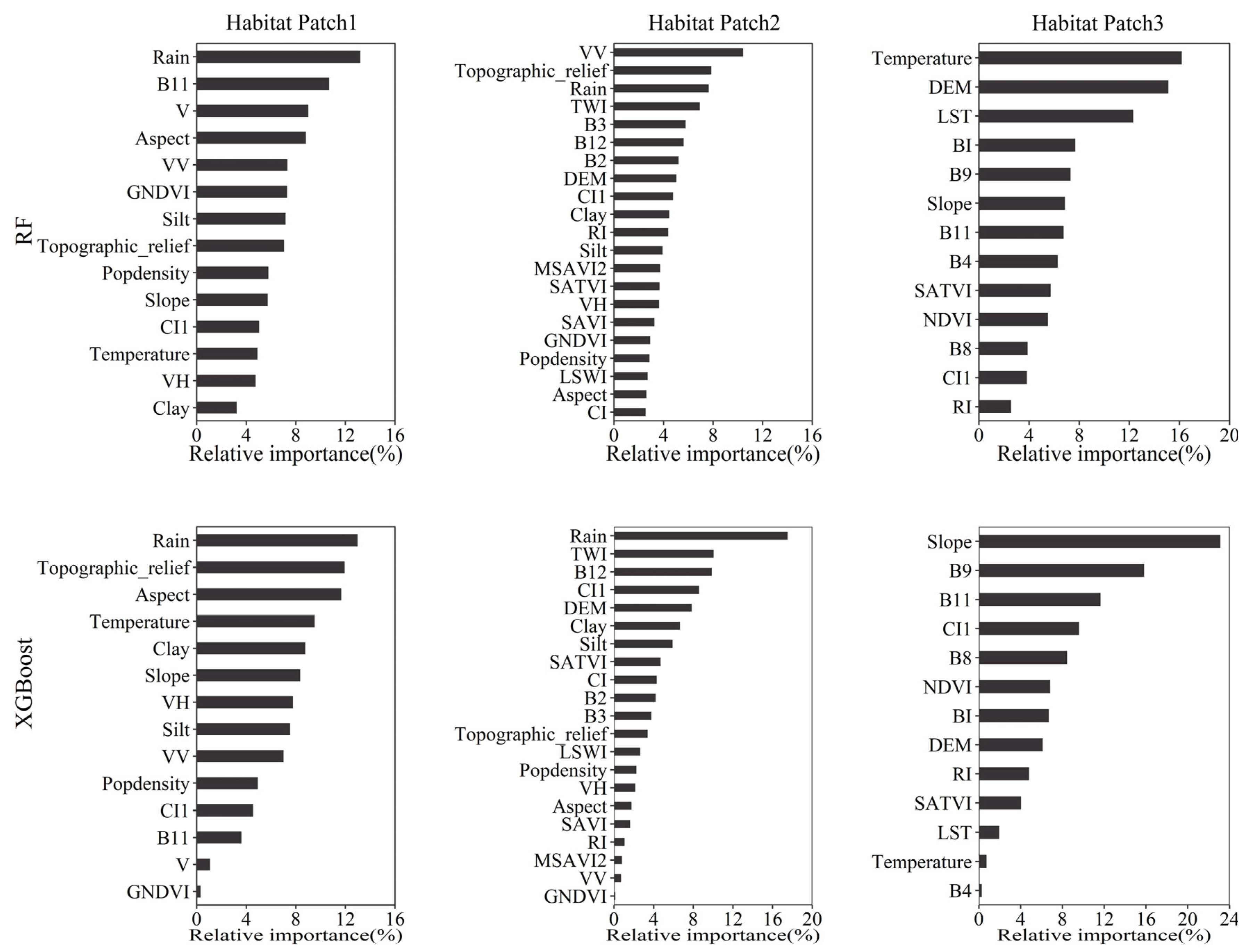
4.1. Variable Importance

The relative importance of covariates filtered through the GA is shown in Figure 7. To improve the comparability of the factors, variable importance was standardized to 100% using a scaling technique [67]. The relative importance of each variable varied according to the RF and XGBoost techniques. For the Habitat Patch 1 area, precipitation, aspect, and temperature were important predictor variables; precipitation and TWI were important variables in the Habitat Patch 2 area; and terrain factors were important to both. The results indicate that climate and topography had a prominent influence on the spatial variance in the SOC. For both the RF (Habitat Patch 2) and XGBoost (Habitat Patch 1 and Habitat Patch 3) models, climate variables ranked among the top three predictors of SOC spatial variation. In particular, for Habitat Patch 3, temperature had the highest explanatory power for the SOC simulation in the Habitat Patch 3 area, which was mainly covered forest.

The intimate relationship between climatic conditions and soil moisture has a major impact on vegetation growth and its net primary productivity [68]. The storage and decomposition of SOC is significantly and widely influenced by climatic factors. Most importantly, climate warming helps microorganisms to accelerate the decomposition of SOC [69]. The SOC content exhibited an augmentation trend in association with precipitation and clay content, while experiencing a decrement in correlation with temperature. The significance of these governing factors manifested a depth-dependent transition, wherein climatic influences predominated in superficial strata, while clay content assumed a dominant role in deeper layers. This shift in control mechanisms is posited to be attributable to escalating proportions of slowly cycling SOC fractions at greater depths [70]. In this study, temperature and precipitation ranked among the top in different machine learning models across different habitat patches. Therefore, in future studies, different climate conditions should be considered more closely, and more sampling sites and socioeconomic factors should be collected to facilitate the prediction of the SOC content and the accurate characterization of its heterogeneous spatial distribution.

In addition, remote sensing imagery also showed its importance in predicting SOC content, including both optical remote sensing data and SAR data (one of microwave remote sensing data). Spectral reflectance, derived indices, and polarization data were effectively used in this study, which is consistent with previous research [71,72,73]. The close relationship between soil and vegetation is the theoretical basis for conducting SOC remote-sensing inversion. In particular, the vegetation index has the potential to effectively reflect variations in soil characteristics [74]. In addition, the water index shows increased sensitivity to variations in soil moisture; the spectral reflectance and the vegetation index are sensitive to the change in soil texture. The adaptability of the backscatter coefficient to changes in both land surface conditions and soil moisture content is a requirement for the use of SAR data in modeling applications [75,76]. The ability of Sentinel-1 imagery to accurately capture features associated with transient changes in vegetation is thought to explain its potential utility for predicting soil quality [77]. However, in this study, SAR data were not used to estimate the SOC content in the Habitat Patch 3 area. Reasons for this may include that the soil’s surface complexity and high spatial heterogeneity increased the noise of the backscatter coefficient.

Topography is a critical determinant in the complex process of soil formation, which can affect hydrological conditions and control the flow of sediments and water [78]. As key predictor variables, elevation and other derived indicators (e.g., aspect, slope, and TWI) significantly affect soil properties and have been frequently utilized for digital soil mapping. The role that slopes play in the spatial variability of SOC is through their impact on the dynamics of water and matter transport and accumulation [79]. The TWI can identify soil moisture gradients and holds great promise for predicting various soil properties [80].

4.2. Geographic Characteristics of the SOC Map and the Uncertainty

The prediction map of the SOC content had similar characteristics to the SoilGrids product [81]. The high SOC content was concentrated in the forest and high elevation regions in the eastern part of the study area. The low SOC content values were mainly located in the farmland and low elevation regions in the western of part the study area. These results were somewhat consistent with the findings of [82], who observed increased SOC levels in forest, in contrast to decreased SOC levels in farmland. Due to the increasing organic matter breakdown and loss through erosion and cultivation, the authors in [83] discovered that the SOC content in forests was higher than that in farmland. The stocks of SOC content increase with increasing elevation [84]. The potential effects of differences in elevation gradients on soil carbon dynamics are mediated by their complex interactions with environmental variables, including vegetation cover, temperature, and precipitation. Abundant vegetative litter causes SOC to accumulate, and the cold climate causes SOC to decompose at a slow rate.

Uncertainties of outcomes are associated with various factors, such as geographic environment characteristics, field sampling numbers, and the quality of data. High uncertainty existed in the Habitat Patch 3 area with dense forest cover and high elevation, and the predication accuracy increase extent was lowest compared to Habitat Patch 1 and Habitat Patch 2. Due to the inaccessibility of some locations, the spatial representativeness of sampling points will decrease. To some extent, it will affect the rationality of building the model and ultimately decrease the estimation accuracy of the SOC. In addition, human activities such as farmland planting and building construction have interrupted the natural area which can be proved from the land cover type distribution map (Figure 1b).

4.3. Limitations and Perspective

We acknowledge the limitation of the modest sample size examined, which may limit the precision of the model’s predictive ability. In scenarios involving complex interdependencies within models, the choice of a larger sample size is typically optimal. The soil prediction framework encompasses multiple facets, including soil properties, covariates, and intricate relationships within the model, requiring an extensive data set. The prevalence of limited sample sizes in soil research is a pervasive phenomenon, as it is largely attributed to the time-consuming nature of soil surveys. Encrypted additional sampling in areas of high uncertainty can improve simulation performance while saving costs.

The complexity of soil formation is an acknowledged fact. In this study, the model constructed based on set trees is only an empirical simplified expression of the soil genesis mechanism, which can only simulate the interaction between and comprehensive effects of various soil forming factors to a certain extent. In addition, considering that machine learning methods essentially rely on existing data for prediction, there is a risk that the prediction results may not reflect the actual situation in regions lacking sample data in geographic and/or feature spaces. Therefore, incorporating the expertise of soil survey experts as a supplement can effectively complement and improve data-driven methods.

Soil moisture plays a critical role in the backscattering response of the surface [85], and its variations directly cause corresponding changes in the backscattering coefficient. Especially in coastal environments, changes in soil moisture are often closely related to precipitation processes and tidal activity. Although this study did not specifically investigate the correlation between soil moisture and backscatter measurements at different time points, the C-band signal of the Sentinel-1 data is trusted by us because it mainly reflects information on the top layer of the vegetation canopy. It is worth noting that soil moisture may indirectly affect the observations by enhancing the volume scattering effect [86]. In addition, the observed differences in backscatter between different soil moisture locations may also be due to dynamic changes in vegetation biomass.

Due to the fact that this study mainly focuses on the feasibility of predicting and mapping methods at the patch scale, the exploration, considering the availability of data, only predicted the SOC content in small areas of the southwestern karst valley area and did not study the applicability of its method in larger-scale areas. Therefore, in the future, larger-scale soil attribute prediction mapping based on patch partitioning methods can be designed for exploration.

5. Conclusions

In this study, field survey SOC data and several topographic, climatic, and remote sensing data were used to build an SOC estimation model. The PAM algorithm was used to divide the study area into three distinct regions. The results showed that three sub-earth surface units (Habitat Patch 1, Habitat Patch 2, and Habitat Patch 3) were created. The SOC spatial distribution was identified based on the prediction results using the RF (for Habitat Patch 2) and XGBoost algorithms (Habitat Patch 1 and Habitat Patch 3). The simulation accuracy of Habitat Patch 1, Habitat Patch 2, and Habitat Patch 3 using the corresponding models was higher than that of the whole study area with one model. The R² increased by 6.8% ~ 25%, and the RMSE decreased by 9.4% ~ 33.6%. Terrain and climate factors were the main variables explaining the spatial variation in the SOC. Habitat Patch 3 (mainly covered forest) had a high SOC prediction value, but the SOC prediction uncertainty was relatively higher with higher human activity and lower representativeness of sampling sites.

References

1. Koarashi, J.; Atarashi Andoh, M.; Ishizuka, S.; Miura, S.; Saito, T.; Hirai, K. Quantitative aspects of heterogeneity in soil organic matter dynamics in a cool-temperate Japanese beech forest: A radiocarbon-based approach. Glob. Chang. Biol. 2009, 15, 631–642. [Google Scholar] [CrossRef]
2. Lal, R. Sequestration of atmospheric CO2 in global carbon pools. Energy Environ. Sci. 2008, 1, 86–100. [Google Scholar] [CrossRef]
3. Parras-Alcántara, L.; Lozano-García, B.; Keesstra, S.; Cerdà, A.; Brevik, E.C. Long-term effects of soil management on ecosystem services and soil loss estimation in olive grove top soils. Sci. Total Environ. 2016, 571, 498–506. [Google Scholar] [CrossRef] [PubMed]
4. Post, W.M.; Peng, T.; Emanuel, W.R.; King, A.W.; Dale, V.H.; DeAngelis, D.L. The global carbon cycle. Am. Sci. 1990, 78, 310–326. [Google Scholar]
5. Lal, R. Soil carbon sequestration impacts on global climate change and food security. Science 2004, 304, 1623–1627. [Google Scholar] [CrossRef] [PubMed]
6. Liang, Q.; Liu, M. An automatic site survey approach for indoor localization using a smartphone. IEEE Trans. Autom. Sci. Eng. 2019, 17, 191–206. [Google Scholar] [CrossRef]
7. Kheir, R.B.; Greve, M.H.; Bøcher, P.K.; Greve, M.B.; Larsen, R.; McCloy, K. Predictive mapping of soil organic carbon in wet cultivated lands using classification-tree based models: The case study of Denmark. J. Environ. Manag. 2010, 91, 1150–1160. [Google Scholar] [CrossRef]
8. Moore, I.D.; Gessler, P.E.; Nielsen, G.; Peterson, G.A. Soil attribute prediction using terrain analysis. Soil Sci. Soc. Am. J. 1993, 57, 443–452. [Google Scholar] [CrossRef]
9. Kaya, F.; Keshavarzi, A.; Francaviglia, R.; Kaplan, G.; Başayiğit, L.; Dedeoğlu, M. Assessing machine learning-based prediction under different agricultural practices for digital mapping of soil organic carbon and available phosphorus. Agriculture 2022, 12, 1062. [Google Scholar] [CrossRef]
10. Wang, T.; Zhou, W.; Xiao, J.; Li, H.; Yao, L.; Xie, L.; Wang, K. Soil Organic Carbon Prediction Using Sentinel-2 Data and Environmental Variables in a Karst Trough Valley Area of Southwest China. Remote Sens. 2023, 15, 2118. [Google Scholar] [CrossRef]
11. Han, J. Spatial clustering methods in data mining: A survey. In Geographic Data Mining and Knowledge Discovery; Taylor and Francis: London, UK, 2001; pp. 188–217. [Google Scholar]
12. Kaufman, L.; Rousseeuw, P.J. Finding Groups in Data: An Introduction to Cluster Analysis; New York John Wiley&Sons: Hoboken, NY, USA, 2009. [Google Scholar]
13. Fahrig, L. Rethinking patch size and isolation effects: The habitat amount hypothesis. J. Biogeogr. 2013, 40, 1649–1663. [Google Scholar] [CrossRef]
14. Fahrig, L.; Arroyo-Rodríguez, V.; Bennett, J.R.; Boucher-Lalonde, V.; Cazetta, E.; Currie, D.J.; Eigenbrod, F.; Ford, A.T.; Harrison, S.P.; Jaeger, J.A. Is habitat fragmentation bad for biodiversity? Biol. Conserv. 2019, 230, 179–186. [Google Scholar] [CrossRef]
15. McBratney, A.B.; Santos, M.M.; Minasny, B. On digital soil mapping. Geoderma 2003, 117, 3–52. [Google Scholar] [CrossRef]
16. Heung, B.; Ho, H.C.; Zhang, J.; Knudby, A.; Bulmer, C.E.; Schmidt, M.G. An overview and comparison of machine-learning techniques for classification purposes in digital soil mapping. Geoderma 2016, 265, 62–77. [Google Scholar] [CrossRef]
17. Zhang, Y.; Sui, B.; Shen, H.; Ouyang, L. Mapping stocks of soil total nitrogen using remote sensing data: A comparison of random forest models with different predictors. Comput. Electron. Agric. 2019, 160, 23–30. [Google Scholar] [CrossRef]
18. Chen, W.; Xie, X.; Wang, J.; Pradhan, B.; Hong, H.; Bui, D.T.; Duan, Z.; Ma, J. A comparative study of logistic model tree, random forest, and classification and regression tree models for spatial prediction of landslide susceptibility. Catena 2017, 151, 147–160. [Google Scholar] [CrossRef]
19. Ain, Q.U.; Aleksandrova, A.; Roessler, F.D.; Ballester, P.J. Machine-learning scoring functions to improve structure-based binding affinity prediction and virtual screening. Wiley Interdiscip. Rev. Comput. Mol. Sci. 2015, 5, 405–424. [Google Scholar] [CrossRef] [PubMed]
20. Reddy, N.N.; Das, B.S. Digital soil mapping of key secondary soil properties using pedotransfer functions and Indian legacy soil data. Geoderma 2023, 429, 116265. [Google Scholar] [CrossRef]
21. Huang, S.; Cai, N.; Pacheco, P.P.; Narrandes, S.; Wang, Y.; Xu, W. Applications of support vector machine (SVM) learning in cancer genomics. Cancer Genom. Proteom. 2018, 15, 41–51. [Google Scholar]
22. Zhao, Z.; Chow, T.L.; Rees, H.W.; Yang, Q.; Xing, Z.; Meng, F. Predict soil texture distributions using an artificial neural network model. Comput. Electron. Agric. 2009, 65, 36–48. [Google Scholar] [CrossRef]
23. Yang, J.; Wang, X.; Wang, R.; Wang, H. Combination of convolutional neural networks and recurrent neural networks for predicting soil properties using Vis–NIR spectroscopy. Geoderma 2020, 380, 114616. [Google Scholar] [CrossRef]
24. Lamichhane, S.; Kumar, L.; Wilson, B. Digital soil mapping algorithms and covariates for soil organic carbon mapping and their implications: A review. Geoderma 2019, 352, 395–413. [Google Scholar] [CrossRef]
25. Wang, Y.; Deng, L.; Wu, G.; Wang, K.; Shangguan, Z. Large-scale soil organic carbon mapping based on multivariate modelling: The case of grasslands on the Loess Plateau. Land Degrad. Dev. 2018, 29, 26–37. [Google Scholar] [CrossRef]
26. Zhou, W.; Xiao, J.; Li, H.; Chen, Q.; Wang, T.; Wang, Q.; Yue, T. Soil organic matter content prediction using Vis-NIRS based on different wavelength optimization algorithms and inversion models. J. Soils Sediments 2023, 23, 2506–2517. [Google Scholar] [CrossRef]
27. Grinand, C.; Le Maire, G.; Vieilledent, G.; Razakamanarivo, H.; Razafimbelo, T.; Bernoux, M. Estimating temporal changes in soil carbon stocks at ecoregional scale in Madagascar using remote-sensing. Int. J. Appl. Earth Obs. Geoinf. 2017, 54, 1–14. [Google Scholar] [CrossRef]
28. Gholizadeh, A.; Žižala, D.; Saberioon, M.; Borůvka, L. Soil organic carbon and texture retrieving and mapping using proximal, airborne and Sentinel-2 spectral imaging. Remote Sens. Environ. 2018, 218, 89–103. [Google Scholar] [CrossRef]
29. Zou, X.; Zhu, S.; Mõttus, M. Estimation of canopy structure of field crops using sentinel-2 bands with vegetation indices and machine learning algorithms. Remote Sens. 2022, 14, 2849. [Google Scholar] [CrossRef]
30. Rajah, P.; Odindi, J.; Mutanga, O.; Kiala, Z. The utility of Sentinel-2 Vegetation Indices (VIs) and Sentinel-1 Synthetic Aperture Radar (SAR) for invasive alien species detection and mapping. Nat. Conserv. 2019, 35, 41–61. [Google Scholar] [CrossRef]
31. Yang, R.; Guo, W. Using time-series Sentinel-1 data for soil prediction on invaded coastal wetlands. Environ. Monit. Assess. 2019, 191, 462. [Google Scholar] [CrossRef] [PubMed]
32. Jiang, Z.; Lian, Y.I.; Qin, X. Rocky desertification in Southwest China: Impacts, causes, and restoration. Earth Sci. Rev. 2014, 132, 1–12. [Google Scholar] [CrossRef]
33. Huang, Y.; Lan, Y.; Thomson, S.J.; Fang, A.; Hoffmann, W.C.; Lacey, R.E. Development of soft computing and applications in agricultural and biological engineering. Comput. Electron. Agric. 2010, 71, 107–127. [Google Scholar] [CrossRef]
34. Meersmans, J.; Van Wesemael, B.; Van Molle, M. Determining soil organic carbon for agricultural soils: A comparison between the Walkley & Black and the dry combustion methods (north Belgium). Soil Use Manag. 2009, 25, 346–353. [Google Scholar]
35. Gorelick, N.; Hancher, M.; Dixon, M.; Ilyushchenko, S.; Thau, D.; Moore, R. Google Earth Engine: Planetary-scale geospatial analysis for everyone. Remote Sens. Environ. 2017, 202, 18–27. [Google Scholar] [CrossRef]
36. Wang, M.; Zhang, Z.; Hu, T.; Wang, G.; He, G.; Zhang, Z.; Li, H.; Wu, Z.; Liu, X. An Efficient Framework for Producing Landsat-Based Land Surface Temperature Data Using Google Earth Engine. IEEE J. Sel. Top. Appl. Earth Observ. Remote Sens. 2020, 13, 4689–4701. [Google Scholar] [CrossRef]
37. Laurencelle, J.; Logan, T.; Gens, R. ASF radiometrically terrain corrected ALOS PALSAR products. Alaska Satell. Facil. 2015, 1, 12. [Google Scholar]
38. Liu, F.; Wu, H.; Zhao, Y.; Li, D.; Yang, J.; Song, X.; Shi, Z.; Zhu, A.; Zhang, G. Mapping high resolution national soil information grids of China. Sci. Bull. 2022, 67, 328–340. [Google Scholar] [CrossRef] [PubMed]
39. Liu, F.; Zhang, G.; Song, X.; Li, D.; Zhao, Y.; Yang, J.; Wu, H.; Yang, F. High-resolution and three-dimensional mapping of soil texture of China. Geoderma 2020, 361, 114061. [Google Scholar] [CrossRef]
40. Escadafal, R. Remote sensing of arid soil surface color with Landsat thematic mapper. Adv. Space Res. 1989, 9, 159–163. [Google Scholar] [CrossRef]
41. Hengl, T. A Practical Guide to Geostatistical Mapping; Office for Official Publications of the European Communities: Luxembourg, 2009. [Google Scholar]
42. Tucker, C.J. Red and photographic infrared linear combinations for monitoring vegetation. Remote Sens. Environ. 1979, 8, 127–150. [Google Scholar] [CrossRef]
43. Gitelson, A.A.; Kaufman, Y.J.; Merzlyak, M.N. Use of a green channel in remote sensing of global vegetation from EOS-MODIS. Remote Sens. Environ. 1996, 58, 289–298. [Google Scholar] [CrossRef]
44. Xiao, X.; Zhang, Q.; Braswell, B.; Urbanski, S.; Boles, S.; Wofsy, S.; Moore, B., III; Ojima, D. Modeling gross primary production of temperate deciduous broadleaf forest using satellite images and climate data. Remote Sens. Environ. 2004, 91, 256–270. [Google Scholar] [CrossRef]
45. Qi, J.; Kerr, Y.; Chehbouni, A. External Factor Consideration in Vegetation Index Development; NASA: Val D’Isere, France, 1994.
46. Pouget, M.; Madeira, J.; Le Floc, H.E.; Kamal, S. Caracteristiques spectrales des surfaces sableuses de la region cotiere nord-ouest de l’Egypte: Application aux donnees satellitaires SPOT. In Caractérisation et Suivi des Milieux Terrestres en Régions Arides et Tropicales, Proceedings of the 2e’me Journées Télédétection; ORSTOM: Bondy, Japan, 1991; pp. 27–38. [Google Scholar]
47. Marsett, R.C.; Qi, J.; Heilman, P.; Biedenbender, S.H.; Watson, M.C.; Amer, S.; Weltz, M.; Goodrich, D.; Marsett, R. Remote sensing for grassland management in the arid southwest. Rangel. Ecol. Manag. 2006, 59, 530–540. [Google Scholar] [CrossRef]
48. Huete, A.R. A soil-adjusted vegetation index (SAVI). Remote Sens. Environ. 1988, 25, 295–309. [Google Scholar] [CrossRef]
49. Nellis, M.D.; Briggs, J.M. Transformed vegetation index for measuring spatial variation in drought impacted biomass on Konza Prairie, Kansas. Trans. Kans. Acad. Sci. 1992, 95, 93–99. [Google Scholar] [CrossRef]
50. Jordan, C.F. Derivation of leaf-area index from quality of light on the forest floor. Ecology 1969, 50, 663–666. [Google Scholar] [CrossRef]
51. Holland, J.H. Adaptation in Natural and Artificial Systems; University of Michigan Press: Ann Arbor, MI, USA, 1975. [Google Scholar]
52. Welikala, R.A.; Fraz, M.M.; Dehmeshki, J.; Hoppe, A.; Tah, V.; Mann, S.; Williamson, T.H.; Barman, S.A. Genetic algorithm based feature selection combined with dual classification for the automated detection of proliferative diabetic retinopathy. Comput. Med. Imaging Graph. 2015, 43, 64–77. [Google Scholar] [CrossRef] [PubMed]
53. Kuhn, M. Building predictive models in R using the caret package. J. Stat. Softw. 2008, 28, 1–26. [Google Scholar] [CrossRef]
54. Breiman, L. Random forests. Mach. Learn. 2001, 45, 5–32. [Google Scholar] [CrossRef]
55. Hansen, L.K.; Salamon, P. Neural network ensembles. IEEE Trans. Pattern Anal. Mach. Intell. 1990, 12, 993–1001. [Google Scholar] [CrossRef]
56. Chen, T.; Guestrin, C. Xgboost: A scalable tree boosting system. In Proceedings of the 22nd ACM SIGKDD International Conference on Knowledge Discovery and Data Mining, San Francisco, CA, USA, 13–17 August 2016. [Google Scholar]
57. Fan, J.; Wang, X.; Wu, L.; Zhou, H.; Zhang, F.; Yu, X.; Lu, X.; Xiang, Y. Comparison of Support Vector Machine and Extreme Gradient Boosting for predicting daily global solar radiation using temperature and precipitation in humid subtropical climates: A case study in China. Energy Convers. Manag. 2018, 164, 102–111. [Google Scholar] [CrossRef]
58. Yagli, G.M.; Yang, D.; Srinivasan, D. Automatic hourly solar forecasting using machine learning models. Renew. Sustain. Energy Rev. 2019, 105, 487–498. [Google Scholar] [CrossRef]
59. Rossel, R.V.; McGlynn, R.N.; McBratney, A.B. Determining the composition of mineral-organic mixes using UV–vis–NIR diffuse reflectance spectroscopy. Geoderma 2006, 137, 70–82. [Google Scholar] [CrossRef]
60. Rojas, R.; Feyen, L.; Dassargues, A. Conceptual model uncertainty in groundwater modeling: Combining generalized likelihood uncertainty estimation and Bayesian model averaging. Water Resour. Res. 2008, 44, W12418. [Google Scholar] [CrossRef]
61. Malone, B.P.; Styc, Q.; Minasny, B.; McBratney, A.B. Digital soil mapping of soil carbon at the farm scale: A spatial downscaling approach in consideration of measured and uncertain data. Geoderma 2017, 290, 91–99. [Google Scholar] [CrossRef]
62. Zeraatpisheh, M.; Garosi, Y.; Owliaie, H.R.; Ayoubi, S.; Taghizadeh-Mehrjardi, R.; Scholten, T.; Xu, M. Improving the spatial prediction of soil organic carbon using environmental covariates selection: A comparison of a group of environmental covariates. Catena 2022, 208, 105723. [Google Scholar] [CrossRef]
63. Adhikari, K.; Hartemink, A.E. Digital mapping of topsoil carbon content and changes in the Driftless Area of Wisconsin, USA. Soil Sci. Soc. Am. J. 2015, 79, 155–164. [Google Scholar] [CrossRef]
64. Ohlmacher, G.C.; Davis, J.C. Using multiple logistic regression and GIS technology to predict landslide hazard in northeast Kansas, USA. Eng. Geol. 2003, 69, 331–343. [Google Scholar] [CrossRef]
65. Dong, L.; Zeng, W.; Wang, A.; Tang, J.; Yao, X.; Wang, W. Response of soil respiration and its components to warming and dominant species removal along an elevation gradient in alpine meadow of the Qinghai–Tibetan plateau. Environ. Sci. Technol. 2020, 54, 10472–10482. [Google Scholar] [CrossRef]
66. Lal, R. Soil carbon sequestration to mitigate climate change. Geoderma 2004, 123, 1–22. [Google Scholar] [CrossRef]
67. Ottoy, S.; Van Meerbeek, K.; Sindayihebura, A.; Hermy, M.; Van Orshoven, J. Assessing top-and subsoil organic carbon stocks of Low-Input High-Diversity systems using soil and vegetation characteristics. Sci. Total Environ. 2017, 589, 153–164. [Google Scholar] [CrossRef] [PubMed]
68. Wang, B.; Waters, C.; Orgill, S.; Gray, J.; Cowie, A.; Clark, A.; Liu, D.L. High resolution mapping of soil organic carbon stocks using remote sensing variables in the semi-arid rangelands of eastern Australia. Sci. Total Environ. 2018, 630, 367–378. [Google Scholar] [CrossRef]
69. Schuur, E.A.; McGuire, A.D.; Schädel, C.; Grosse, G.; Harden, J.W.; Hayes, D.J.; Hugelius, G.; Koven, C.D.; Kuhry, P.; Lawrence, D.M. Climate change and the permafrost carbon feedback. Nature 2015, 520, 171–179. [Google Scholar] [CrossRef]
70. Jobbágy, E.G.; Jackson, R.B. The vertical distribution of soil organic carbon and its relation to climate and vegetation. Ecol. Appl. 2000, 10, 423–436. [Google Scholar] [CrossRef]
71. Bao, Y.; Lin, L.; Wu, S.; Deng, K.A.K.; Petropoulos, G.P. Surface soil moisture retrievals over partially vegetated areas from the synergy of Sentinel-1 and Landsat 8 data using a modified water-cloud model. Int. J. Appl. Earth Obs. Geoinf. 2018, 72, 76–85. [Google Scholar] [CrossRef]
72. Nguyen, T.T.; Pham, T.D.; Nguyen, C.T.; Delfos, J.; Archibald, R.; Dang, K.B.; Hoang, N.B.; Guo, W.; Ngo, H.H. A novel intelligence approach based active and ensemble learning for agricultural soil organic carbon prediction using multispectral and SAR data fusion. Sci. Total Environ. 2022, 804, 150187. [Google Scholar] [CrossRef] [PubMed]
73. Zhou, T.; Geng, Y.; Chen, J.; Liu, M.; Haase, D.; Lausch, A. Mapping soil organic carbon content using multi-source remote sensing variables in the Heihe River Basin in China. Ecol. Indic. 2020, 114, 106288. [Google Scholar] [CrossRef]
74. Mahmoudabadi, E.; Karimi, A.; Haghnia, G.H.; Sepehr, A. Digital soil mapping using remote sensing indices, terrain attributes, and vegetation features in the rangelands of northeastern Iran. Environ. Monit. Assess. 2017, 189, 500. [Google Scholar] [CrossRef] [PubMed]
75. Shi, J.; Wang, J.; Hsu, A.Y.; O’Neill, P.E.; Engman, E.T. Estimation of bare surface soil moisture and surface roughness parameter using L-band SAR image data. IEEE Trans. Geosci. Remote Sens. 1997, 35, 1254–1266. [Google Scholar]
76. Wagner, W.; Scipal, K.; Pathe, C.; Gerten, D.; Lucht, W.; Rudolf, B. Evaluation of the agreement between the first global remotely sensed soil moisture data with model and precipitation data. J. Geophys. Res. Atmos. 2003, 108, 4611. [Google Scholar] [CrossRef]
77. Yang, R.; Guo, W.; Zheng, J. Soil prediction for coastal wetlands following Spartina alterniflora invasion using Sentinel-1 imagery and structural equation modeling. Catena 2019, 173, 465–470. [Google Scholar] [CrossRef]
78. Li, Q.; Yue, T.; Wang, C.; Zhang, W.; Yu, Y.; Li, B.; Yang, J.; Bai, G. Spatially distributed modeling of soil organic matter across China: An application of artificial neural network approach. Catena 2013, 104, 210–218. [Google Scholar] [CrossRef]
79. Tsui, C.; Chen, Z.; Hsieh, C. Relationships between soil properties and slope position in a lowland rain forest of southern Taiwan. Geoderma 2004, 123, 131–142. [Google Scholar] [CrossRef]
80. Siewert, M.B. High-resolution digital mapping of soil organic carbon in permafrost terrain using machine learning: A case study in a sub-Arctic peatland environment. Biogeosciences 2018, 15, 1663–1682. [Google Scholar] [CrossRef]
81. Hengl, T.; Mendes De Jesus, J.; Heuvelink, G.B.M.; Ruiperez Gonzalez, M.; Kilibarda, M.; Blagotić, A.; Shangguan, W.; Wright, M.N.; Geng, X.; Bauer-Marschallinger, B.; et al. SoilGrids250m: Global gridded soil information based on machine learning. PLoS ONE 2017, 12, e169748. [Google Scholar] [CrossRef] [PubMed]
82. Were, K.; Bui, D.T.; Dick, Ø.B.; Singh, B.R. A comparative assessment of support vector regression, artificial neural networks, and random forests for predicting and mapping soil organic carbon stocks across an Afromontane landscape. Ecol. Indic. 2015, 52, 394–403. [Google Scholar] [CrossRef]
83. Wang, S.; Adhikari, K.; Wang, Q.; Jin, X.; Li, H. Role of environmental variables in the spatial distribution of soil carbon (C), nitrogen (N), and C: N ratio from the northeastern coastal agroecosystems in China. Ecol. Indic. 2018, 84, 263–272. [Google Scholar] [CrossRef]
84. Tsui, C.; Tsai, C.; Chen, Z. Soil organic carbon stocks in relation to elevation gradients in volcanic ash soils of Taiwan. Geoderma. 2013, 209, 119–127. [Google Scholar] [CrossRef]
85. Ulaby, F.T.; Moore, R.K.; Fung, A.K. Microwave Remote Sensing: Active and Passive. Volume 2-Radar Remote Sensing and Surface Scattering and Emission Theory; Addison-Wesley: Reading, MA, USA, 1982. [Google Scholar]
86. Barrett, B.; Nitze, I.; Green, S.; Cawkwell, F. Assessment of multi-temporal, multi-sensor radar and ancillary spatial data for grasslands monitoring in Ireland using machine learning approaches. Remote Sens. Environ. 2014, 152, 109–124. [Google Scholar] [CrossRef]
Figure 1. The locations of sampling points and the study site. (a) the range of elevation; (b) land use/land cover map.
Remotesensing 16 00688 g001
Figure 2. The flowchart of this study.
Remotesensing 16 00688 g002
Figure 3. Frequency histogram and statistics of SOC content.
Remotesensing 16 00688 g003
Figure 4. SOC content in different habitat patches.
Remotesensing 16 00688 g004
Figure 5. Results of the study area delineation.
Remotesensing 16 00688 g005
Figure 6. Predicted map (a) and uncertainty (b) of SOC content (Habitat Patch 1 and Habitat Patch 3 using XGBoost, Habitat Patch 2 using RF).
Remotesensing 16 00688 g006
Figure 7. Relative importance of the auxiliary variables on the basis of RF and XGBoost models in different habitat patches.
Remotesensing 16 00688 g007