Article

Soil Organic Carbon Prediction Using Sentinel-2 Data and Environmental Variables in a Karst Trough Valley Area of Southwest China

1
Chongqing Jinfo Mountain Karst Ecosystem National Observation and Research Station, School of Geographical Sciences, Southwest University, Chongqing 400715, China
2
Chongqing Engineering Research Center for Remote Sensing Big Data Application, School of Geographical Sciences, Southwest University, Chongqing 400715, China
3
State Key Laboratory of Resources and Environmental Information System, Institute of Geographic Sciences and Natural Resources Research, CAS, Beijing 100101, China
4
Beijing Piesat Information Technology Co., Beijing 100195, China
5
Chongqing Municipal Public Security Bureau Special Weapon and Tactics Police Aviation Management Office, Chongqing 401147, China
*
Author to whom correspondence should be addressed.
Remote Sens. 2023, 15(8), 2118; https://doi.org/10.3390/rs15082118
Submission received: 22 March 2023 / Revised: 12 April 2023 / Accepted: 14 April 2023 / Published: 17 April 2023
(This article belongs to the Special Issue Remote Sensing for Land System Mapping and Monitoring)

Abstract

:
Climate change is closely linked to changes in soil organic carbon (SOC) content, which affects the terrestrial carbon cycle. Consequently, it is essential for carbon accounting and sustainable soil management to predict SOC content accurately. Although there has been an extensive utilization of optical remote sensing data and environmental factors to predict SOC content, few studies have explored their applicability in karst areas. Therefore, it remains unclear how SOC content can be accurately simulated in these areas. In this study, 160 soil samples, 8 environmental covariates and 14 optical remote sensing variables were used to build SOC content prediction models. Three machine learning models, i.e., support vector machine (SVM), random forest (RF) and extreme gradient boosting (XGBoost), were applied for each of three land use classes, including the entire study area, as well as farmland and forest areas. The variables with the greatest influence were the optical remote sensing bands, derived indices, as well as precipitation and temperature for forest areas, and optical remote sensing band11 and Pop-density for farmland. The results from this study suggest that RF and XGBoost are superior to SVM in prediction accuracy. Additionally, the simulation accuracy of the RF model for the forest areas (R2 = 0.32, RMSE = 6.81, MAE = 5.63) and of the XGBoost model for farmland areas (R2 = 0.28, RMSE = 4.03, MAE = 3.27) was the greatest. The prediction model based on different land use types could obtain a higher simulation accuracy than that based on the whole study area. These findings provide new insights for the estimation of SOC content with high precision in karst areas.

Graphical Abstract

1. Introduction

Factors such as climate change and human disturbance can have a significant impact on soil, as it is a vital element of the environment with high sensitivity [1]. On land, the most significant amount of organic carbon is stored in the soil [2], which plays a vital role in terrestrial ecosystem functioning through its structure and quality. A previous research has shown that the global reservoir of soil organic carbon (SOC) exceeds the amount stored in the atmosphere and vegetation by a factor of two to three [3], respectively. Changes in SOC levels, even at minimal levels, can cause significant fluctuations in atmospheric CO2 levels. The soil has the ability to increase carbon uptake, which can potentially mitigate CO2 emissions and slow the progression of climate change [4]. Previous studies have shown that the adoption of good agricultural practices on degraded land can significantly increase its capacity to store carbon. This, in turn, can increase crop production and effectively contribute to maintaining food security [5,6]. Therefore, in the context of climate warming, soil degradation and food security, the measurement and monitoring of SOC levels over large regions is of paramount importance.
For predicting SOC content, the traditional method of field sampling and laboratory testing is both difficult and costly for large areas with large numbers of sampling points [7]. However, digital soil mapping (DSM) can be an effective and low-cost tool for predicting large-scale SOC distributions [8,9]. The majority of DSM methods is based on soil landscape models and is built using soil properties and environmental variables quantitatively [10,11]. The prediction models mainly include statistical regression and machine learning methods. Among the statistical regression models, multiple linear regression and partial least squares regression (PLSR) are most widely used. In addition, the use of machine learning algorithms has been extensively applied to the study of SOC estimation and its cartographic representation, including support vector machine (SVM), random forest (RF), artificial neural network (ANN) [12] and extreme gradient boosting (XGBoost) [13]. Previous studies comparing six machine learning methods found that the estimation accuracy of Deep Learning Neural Networks (DNN), RF and XGBoost was higher than that of SVM, ANN and Cubist [13,14,15], and the stacking ensemble learning model achieved the highest prediction accuracy overall. Here, we chose SVM, RF and XGBoost as the simulation models for SOC content prediction.
The prediction of soil properties such as SOC content requires the use of sufficient environmental variables, for example, topography, climate, soil texture, vegetation or human interference (land use and land cover, population, etc.). These factors affect the formation and change of the soil and are typically used in SOC content prediction [16,17,18]. Although we cannot directly obtain the soil spectral information in a vegetation cover area, the interaction between vegetation and soil, such as vegetation influencing soil biochemical processes and the distribution of vegetation being governed by soil properties [19], provides an important theoretical basis for the inversion of soil properties using optical remote sensing data. As another important data source, remote sensing imagery is also widely used for predicting SOC levels and significantly affects the ability to predict SOC content [20]. Currently, predicting SOC content using optical remote sensing data has received considerable attention due to its ubiquitous application. The band reflectance [21] vegetation index [22,23] and, especially, the NDVI [24,25] are most widely used in DSM in combination with other environment variables. In recent years, synthetic aperture radar (SAR) has also been used in the prediction of SOC content, as it has the advantage of operating continuously in all weather conditions. For example, a previous study found that Sentinel-1 displayed good potential for application in digital soil mapping [12], while Poggio and Gimona [26] and Yang and Guo [27] also found that in eastern China, the use of the backscatter coefficient derived from Sentinel-1 imagery represents a promising approach for the comprehensive characterization of soil properties, especially with respect to their spatial variability. Above all, with the emergence of spatiotemporal big data, many open-source remote sensing data and basic geographic data have become more readily available and have greatly enriched the input variables of SOC estimation models. Using data such as these, researchers have now successfully predicted and mapped SOC globally [28] and the spatial variation of soil properties [10].
Covering an area of about 22 million km2, karst landforms occupy about 15% of the earth’s surface [29]. In southwest China, they account for about 26% (0.51 million km2) of the total land area [30]. Karst landforms are most easily defined by their topographic and geomorphological features, soil development levels, hydrothermal and vegetation conditions. The typical characteristics of karst areas are broken terrain, a thin soil layer, exposed rocks dividing the soil mass into pieces and serious water and soil loss. These features result in a poor immunity to interference and low stability in these areas [29]. Due to their complex geological and topographic conditions, SOC content in karst areas exhibits an obvious spatial heterogeneity [31]. Moreover, with the rapid economic development and explosive population growth in recent years, excessive human disturbance has caused soil desertification and significant variation in SOC content [32]. These factors inevitably influence the properties of the soil and the carbon cycle and thus make it difficult to assess the dynamics of SOC storage in these areas. However, previous studies on the content of SOC or its dynamics mainly focused on a single driving factor [33]. In karst areas, complex landforms, fragmented topography, various land use types and soil types cause the soil to follow a discontinuous and patching pattern [34]. In karst areas, the variability of SOC content is strongly influenced by different conditions, resulting in a high degree of spatial heterogeneity. Predicting SOC levels in such regions requires the consideration of the dominant driving factors, which vary widely. Therefore, by exploring the main driving factors associated with different land use types, the simulation accuracy of SOC content may be increased. The main objectives of this study were: ① to determine the applicability of optical and SAR remote sensing data in predicting SOC content in karst areas; ② to determine whether the prediction model based on different land use types could obtain higher simulation accuracy than that based on the whole study area.

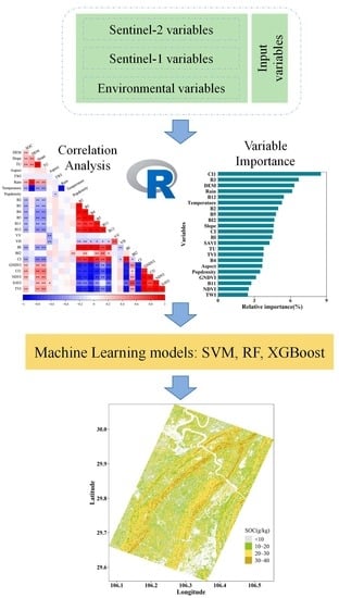
2. Materials and Methods
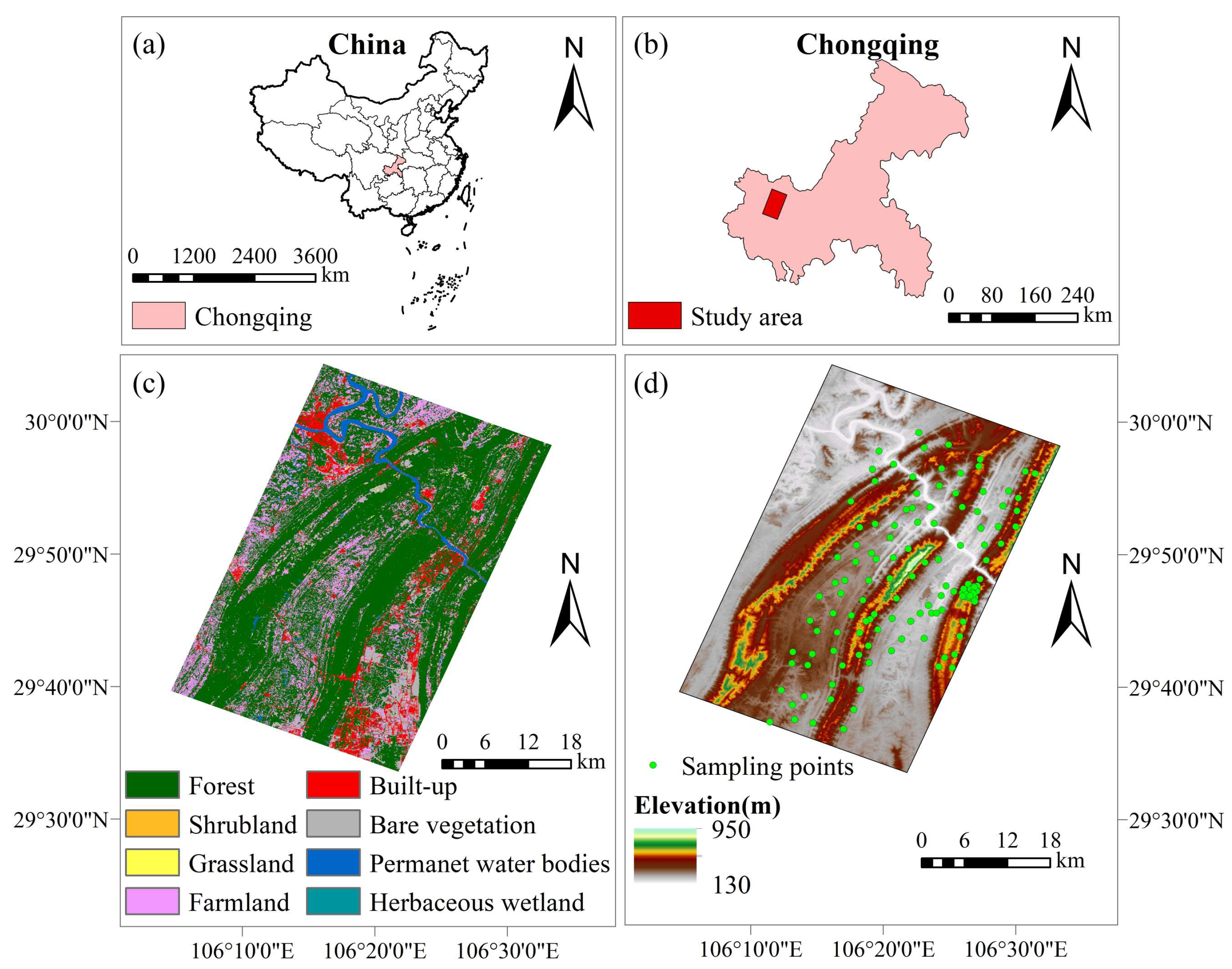
2.1. Study Area

Figure 1 shows the study area, situated in the northwest of Chongqing, China. The climate is humid subtropical with a monsoon flavor and temperatures ranging between 16 and 18 °C. Additionally, the region has an annual precipitation ranging from 1000 to 1350 mm. The study area consists of yellow soil and purple soil zonal types and is characterized by farmland and forest as the main forms of land use. Its altitude ranges from 130 to 950 mm above sea level.

2.2. Sample Data

Field surveys were conducted in January 2020, where sampling points were selected reasonably using Google satellite imagery based on the geographical characteristics of the study area (Figure 1). In this study, the survey methodology involved the selection of a 2 km by 2 km square area as the unit of analysis. Specifically, three plots were systematically sampled from each survey site, with their locations distributed along the diagonal of the square area. At each sampling point, soil samples were collected using the five-point mixed sampling method, and multiple samples were then combined into one sample. Each topsoil sample was taken from a quadrat with five different subsamples selected for analysis. All sampling points were pinpointed using GPS. The soil samples were labeled and sealed after collection. The sampling sites were recorded in detail with regard to land use type, soil texture and vegetation cover. Photographs were taken of the surroundings of the sampling sites. In total, 160 surface soil (0–20 cm) samples were collected and used for analysis.

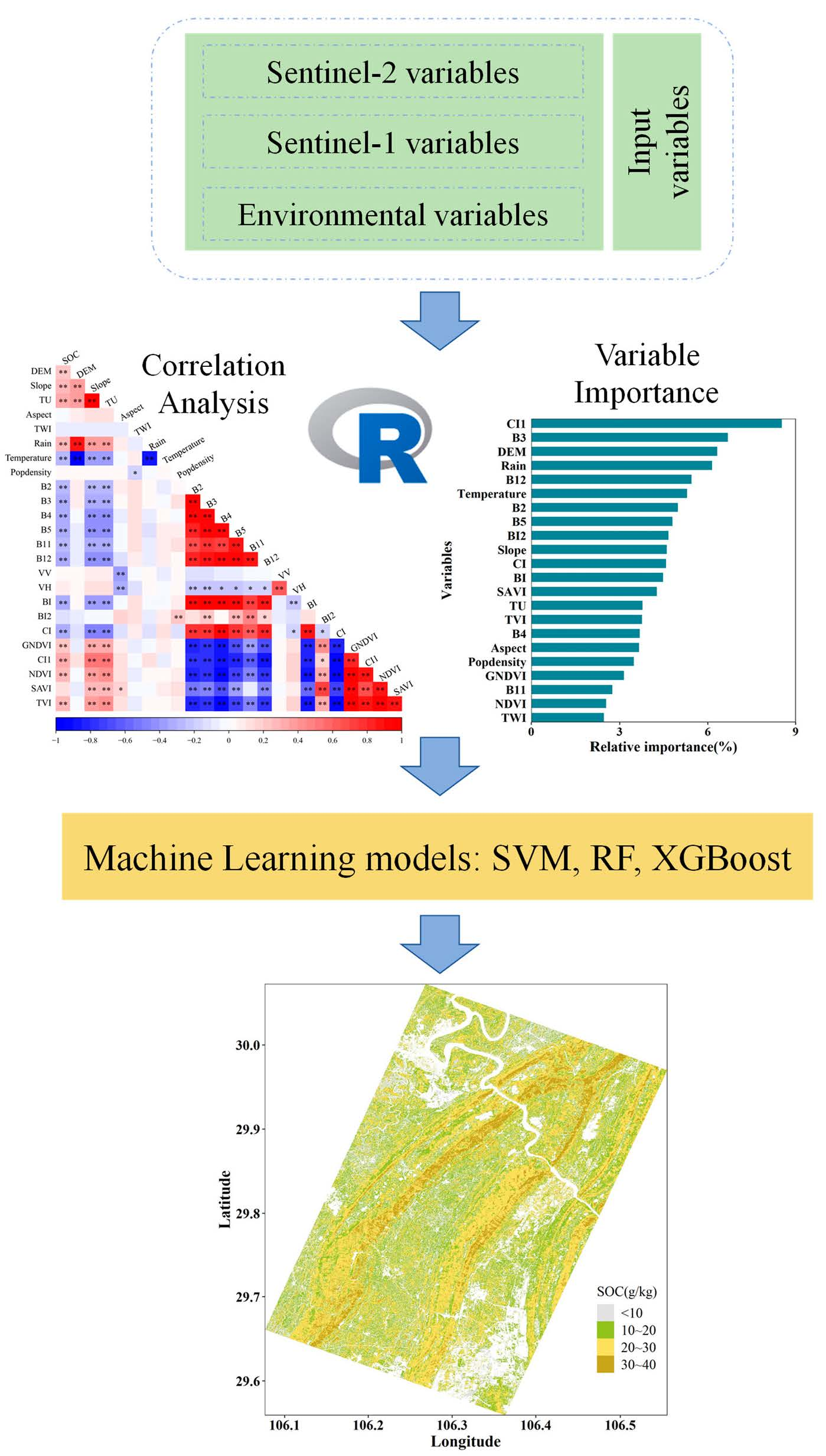
2.3. Driving Variables

All variables were converted to a raster format at 10 m resolution and used to generate the driving variables. Based on these raster data, for each soil sample point, the variables’ pixel values were calculated to build the model.

2.3.1. Environmental Covariates

Environmental variables used for SOC prediction mapping included land use/land cover (LULC), climate and topography variables. The LULC data were provided by the European Space Agency (ESA) (https://viewer.esa-worldcover.org/worldcover/, accessed on 1 March 2022). The ESA WorldCover 10 m 2020 product provided a global land cover map for 2020 at 10 m resolution, developed and validated in near real time based on Sentinel-1 and Sentinel-2 data [35]. The WorldCover product comes with 11 land cover classes (tree cover, shrubland, grassland, cropland, built-up, bare/sparse vegetation, snow and ice, permanent and water bodies, herbaceous wetland, mangroves, moss and lichen) and has been generated in the framework of the ESA WorldCover project, part of the 5th Earth Observation Envelope Programme (EOEP-5) of the European Space Agency. The mean annual temperature and precipitation data for the study area were obtained from the Resources and Environmental Science and Data Center of the Chinese Academy of Sciences (RESDC) (http://www.resdc.cn, accessed on 3 March 2022). The calculation of five topographic variables was performed using the raster calculator in Arcmap12.5 software from the Advanced Land Observing Satellite (ALOS) DEM [36] at 12.5 m spatial resolution, including elevation, terrain undulation, slope, aspect and topographic wetness index (TWI). The population density data were provided by the Socioeconomic Data and Applications Center (https://sedac.ciesin.columbia.edu/data/set/gpw-v4-population-density-rev11, accessed on 5 March 2022) [37].

2.3.2. Remote Sensing Variables

In this study, Sentinel-2A optical data which were downloaded from Google Earth Engine (GEE), were included. The acquisition dates were close to the field data collection dates (January 2020). Sentinel-2A data were acquired from the Multispectral Instrument (MSI) L2A product. The product has been pre-processed by ESA for radiometric calibration, atmospheric correction, etc., so the data reflect the reflectance information at the surface. Nearest neighborhood resampling methods were used to harmonize the spatial resolution. Seven extracted bands and eight calculated spectral indices of Sentinel-2A were included [20,38,39]. In remote sensing, soil texture, mineral composition, soil moisture and organic matter content were considered, all four of which can affect the optical properties of the soil. Thus, for the purpose of retrieving variables indirectly by predicting their interrelationships, several sets of spectral indices were calculated, including vegetation indices (which respond to changes in soil organic matter content sensitively; Jin et al. [40,41] and Liu et al. [42] have recently used these indices to predict soil attributes) and brightness-related indices (sensitive to the soil texture). The employed spectral indices included the Normalized Differences Vegetation Index (NDVI), Transformed Vegetation Index (TVI), Soil-Adjusted Vegetation Index (SAVI), Green Normalized Difference Vegetation Index (GNDVI), Brightness Index (BI), Second Brightness Index (BI2), Color Index (CI) and Clay Index (CI1). Table 1 shows the formulas used to obtain these indices. The details of the Sentinel-2A bands that were utilized are provided in Table 2 [43]. The Sentinel-1 mission provides data from a dual-polarization C-band SAR instrument at 5.405 GHz (C band). This collection includes the S1 Ground Range Detected (GRD) scenes, processed using the Sentinel-1 Toolbox to generate a calibrated, ortho-corrected product. Pre-processed Sentinel-1A SAR data were downloaded from GEE (Table 3). Additionally, VV and VH polarization data were used in this study.

2.4. Prediction Models

The concept of the SVM model was derived from the principles of the statistical learning theory, which were then applied to classification and regression tasks through the process of structural risk minimization [51]. The SVM model benefits from its ability to handle small samples and its nonlinearity and high dimensionality. We utilized the e1071 package within the R software to implement the SVM model. The kernel was set to a radial kernel function using the caret package.
The RF model, a type of algorithm in the field of machine learning, uses ensemble learning. As a big data and nonlinear application, the RF model can reduce the running time and ensure the model accuracy. During the training process, multiple random trees are used in the RF model to generate a unified prediction, effectively combining their individual outputs [16]. A bootstrap sample is utilized from the training data to construct the trees located in the forest, with each tree being distinct. This process helps to avoid overfitting and ensures that the model is robust. The randomForest package in R software was utilized to execute the RF model. The parameters that need to be adjusted using the RF model are ntree and mtry. The ntree was adjusted to 700.
XGBoost is a new ensemble model based on the decision tree approach [52], combining the advantages of regression trees and boosting algorithms. Based on the boosting strategy, XGBoost obtains strong learners from weak learners, improves computing speed through parallel learning and effectively prevents over-fitting. The XGBoost model improves the iterative optimization process and establishes the residual model in the gradient descent direction of the training sample. It also uses Taylor expansion to fit the residual of the loss function model. The learning rate(eta) and maximum depth(max_depth) per tree in XGBoost model were set to 0.3 and 7. We used the grid searching technique provided by the caret package to fine-tune the parameters for all three models. This was achieved by adjusting the values of various parameters and evaluating the performance of the models. The above three models and SOC prediction mapping were implemented in R 4.1.1.

2.5. Model Evaluation

In this study, the models were calibrated by implementing a 10-fold cross-validation using a randomized segmentation technique. For the purpose of evaluating and comparing the SOC prediction accuracy of the models, three commonly used indices were employed, including the root-mean-square error (RMSE), the mean absolute error (MAE) and the coefficient of determination (R2). The indices were calculated using the following equations:
R M S E = 1 n i = 1 n ( P i M i ) 2
M A E = 1 n i = 1 n | P i M i |
R 2 = ( i = 1 n ( M i M ¯ ) ( P i P ¯ ) i = 1 n ( M i M ¯ ) 2 i = 1 n ( P i P ¯ ) 2 ) 2
where Mi and Pi are the measured and predicted values of SOC content (g/kg), M ¯ and P ¯ indicate the mean of the measured and predicted SOC content, n represents the number of soil sampling points.

3. Results

3.1. Descriptive Statistics

The SOC content varied greatly between the farmland and the forest areas (the average values of SOC were 12.68 and 18.15 g/kg), with standard deviation values of 5.30 and 11.48, respectively. A more skew distribution was observed in the overall SOC content (the skewness value was 2.12) than in that of farmland and forest areas (Table 4). The SOC content decreased as soil depth increased. The degree of data discretization also decreased with increasing soil depth (Table 5).

3.2. Correlation of SOC with Driving Variables

Correlation matrices were constructed between Sentinel-1 polarization data, Sentinel-2A data (both bands and derived indices) and SOC to determine the level of significance between soil organic carbon (SOC) content and its drivers, both positive and negative, and to identify the key spectral bands or indices for predicting SOC (Figure 2).
For the whole area, high correlation was observed between SOC and CI, CI1, B12, BI, B4, B5, B3, TU, B2 and Rain. For the forest areas, B12, B11, B5, BI, B4, B3, Rain, CI, B2, Temperature and CI1 were significantly correlated with SOC. For the farmland areas, only Pop-density displayed a significant correlation with SOC.
Note: SOC, soil organic carbon; DEM, elevation; TU, terrain undulation; TWI, topographic wetness index; Rain, mean annual precipitation; Temperature, mean annual temperature; Popdensity, population density; B2, B3, B4, B5, B11, B12 are band 2, band 3, band 4, band 5 and band 12 of Sentinel-2A image.

3.3. Variable Importance and Feature Selection

During the modeling process, the RF model is able to determine the importance of each variable. This importance is related to how much individual variables affect the prediction accuracy. By analyzing these factors, the model can identify which variables have a greater impact on the outcome. The importance of each driving variable is demonstrated in Figure 3, where their relative contributions are depicted. To allow for a comparative analysis between variables, the significance of each variable was normalized to 100%. The normalization of the variables makes it easier to assess their relative importance.
The five main driving variables for the whole study area were CI1, B3, DEM, Rain and B12, with relative importance values of 9%, 7%, 6%, 6% and 5%, respectively. For the forest area, they were B3, B5, B2, B12 and BI 2, with relative importance values of 9%, 7%, 7%, 7% and 6%, respectively. For farmland, they were Popdensity, B11, B5, CI and BI 2, with relative importance values of 8%, 7%, 6%, 6% and 6%, respectively.
Combining the results of the correlation coefficient and the variable importance analyses, the modeling variables chosen were B3, B5, B12, BI, CI, CI1, Rain and DEM for the whole study area. For the forest area, B2, B3, B4, B5, B11, B12, BI, CI1, Rain and Temperature were selected as modeling variables. For the farmland area, Popdensity and B11 were selected as the modeling variables.

3.4. Model Performance

Three models were used to predict SOC content for the overall area, farmland and forest areas. Among all the models tested on the overall samples, the model utilizing the RF technique displayed the greatest precision, which was evidenced by the lowest RMSE (7.35) and MAE (5.74) values, as well as the highest R2 value (0.17). For the forest area, the RF model exhibited superior performance in comparison to the XGBoost model. For the farmland area, the XGBoost model demonstrated superior performance in terms of predicting accuracy, with an R2 value of 0.28, an RMSE value of 4.03, and a MAE value of 3.27. In general, the XGBoost and RF models exhibited notably superior predictive accuracy in comparison to the SVM model, regardless of where the samples were collected. The prediction model based on different land use types could obtain a higher simulation accuracy than that based on the whole study area (Table 6).
Based on the accuracy results of the SOC content simulation, RF was used as the simulation model for the forest area, while XGBoost was selected for farmland.

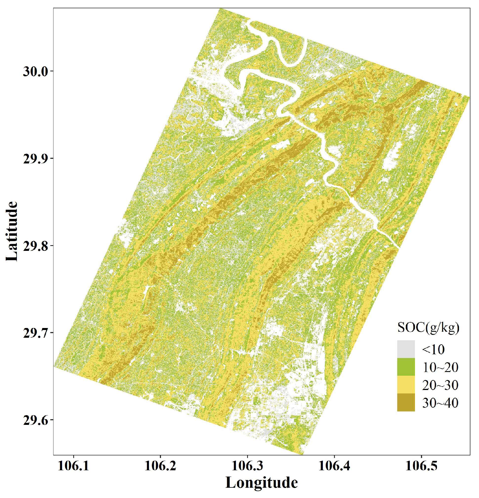
3.5. Predicted Spatial Distribution of SOC Content

In the forest, the distribution of SOC content was mapped using the RF model, while the XGBoost model was used for agricultural areas. This allowed the spatial variation of SOC content in both land cover types to be accurately depicted (Figure 4). Through the analysis conducted, a strong correlation was identified between the elevation and the spatial distribution of SOC content, whose distribution pattern showed similarities to that of the DEM. In the lower valleys, SOC content was notably lower compared to that found in the higher mountainous regions on both sides. This reflected the dominance of the terrain as a driving factor affecting SOC content and its spatial distribution. At higher altitudes, the light conditions are better, and with increased sunshine duration, plant photosynthesis is promoted, thus increasing the input of SOC. At the same time, the higher altitude forms a lower temperature environment, which reduces the decomposition reaction rate of SOC by microorganisms and increases the solid stock of SOC [53,54]. The higher altitude also reflects the relationship between land use and SOC. Dense forests are mostly distributed in higher altitude mountains. The favorable geographical conditions of the forest and its high capacity for carbon sequestration cause their soil organic carbon to increase.
Table 7 presents the statistical analysis for the predicted SOC content. The predicted SOC content was obtained from the cropland and forest areas, and the mean and standard deviation were calculated. In the agricultural areas, the average predicted SOC content was 11.54, with a standard deviation of 3.69, while the forest areas had an average predicted SOC content of 21.85, with a standard deviation of 5.64. These results indicated a significant contrast in predicted SOC content between agricultural and forest plots. Using the XGBoost model, the mean and standard deviation of the predicted SOC content were found to be lower than those of the measured SOC content on the farmland. The result indicated that the estimated level of SOC content had less variability compared to the measured SOC content in agricultural regions. Moreover, the lower valleys are mainly distributed within farmland. Due to the high degree of interference from human activities in these areas, the SOC content may be irreversibly damaged. In this way, the decomposition rate of SOC is accelerated, resulting in a lower SOC content in the low valley areas.

4. Discussion

4.1. Model Performance

The RF and XGBoost models achieved better SOC prediction accuracies than the SVM in this study. This is in line with previous studies [55,56], which found that the BRT and RF models were superior to SVM in prediction accuracy in semi-arid Australia and the Heihe River Basin in China. Similarly, in comparing the simulation accuracy of different models for predicting SOC, evaluating the RF, SVM, Cubist and GLM performances, Gomes et al. [16] concluded that the RF model provided the highest prediction accuracy. Taghizadeh-Mehrjardi et al. [12] employed six machine learning methods to predict SOC content and found that the DNN performed better than the RF and XGBoost models and achieved the average of the neural network, ANN, and Cubist models for arid and sub-humid regions in Iran. Additionally, Zhou et al. [12] found that the BRT and RF models exhibited comparable predictability in estimating the SOC content in the Heihe River Basin in China. Based on the above studies, there is no unique machine learning model which is most suitable for all landscapes. Meanwhile, in this study, we built a prediction model of SOC content based on overall sampling as well as on sampling from the specific land types of forest and farmland. Our results showed that XGBoost performed better (R2 = 0.77) than RF (R2 = 0.66) and SVM (R2 = 0.20) in farmland areas, while RF obtained higher accuracy than XGBoost and SVM in the forest areas and in the overall sampling area (). These results underscore the significance of evaluating and contrasting the predictive power of different models in different landscapes.

4.2. The Driving Factors of SOC Content Prediction Models

A variety of optical remote sensing images have been employed for predicting and mapping soil properties, including Landsat, Sentinel-2A, and others. In this study, the top five driving variables in forest and farmland were band 3, band 5, band 2, band 12 of Sentinel-2A and BI 2, and pop-density, band 11, band 5 of Sentinel-2A, CI and BI 2, respectively. This is in line with the results of a previous study [57], which also found that the explanatory power of variables derived from optical remote sensing was higher than that of climatic and topographic variables. However, for the whole sampling area, the five most important predictor variables were CI1, band 3, DEM, Rain and band 12. These results highlight the significance of the type of land use among the driving factors in predicting SOC. However, some previous studies reported success using SAR data, especially the backscatter coefficients of polarization data derived from multi-temporal Sentinel-1 imagery to predict soil properties [56,58]. In contrast, in the present study, Figure 2 shows that the VV and VH polarization data were weakly correlated with SOC, with a correlation coefficient of less than 0.1. Therefore, we believe that Sentinel-1 imagery was not significantly correlated with SOC content and was not selected as a driving factor for predicting SOC. Factors affecting radar backscatter in agricultural fields include crop biomass, crop structure and soil conditions. Previous research established that the backscatter signal detected by C-band radar is a convolution of the ground backscatter modified by the canopy layer and the backscatter from the canopy itself, involving single and multiple scattering mechanisms and vegetation–ground interactions [59]. The observed soil returns at VH polarization were likely due to the phenomenon of double scattering, with the scattering of waves within the soil medium occurring twice, from the soil and the stem components. This mechanism is thought to exceed the direct backscatter from the soil surface alone. The study area with complex topography and surface landscape destruction made the information obtained from Sentinel-1 image retroreflection cumbersome, and the effective image information underwent interference. Previous studies also observed that high surface roughness and plant type difference increased the difficulty of soil and vegetation scattering simulation [60,61]. Therefore, the spatial heterogeneity of surface roughness and crop planting may increase backscattering in karst areas.
The distribution of soil characteristics is closely associated with geographic features, which are often utilized as a primary predictor in DSM [62,63]. Specifically, in a previous study, elevation had the highest relative importance [10] and was also the most effective driving factor in DSM [64]. This is likely because the local microclimate can be affected by changes in elevation, which in turn can have an indirect effect on the activity of microorganisms, thereby influencing the transformation and decomposition of the soil nutrients [65]. Meanwhile, an obvious significant correlation was observed between elevation and mean annual temperature and precipitation in this study (Figure 2), further suggesting that elevation can affect the regional climate. In addition, other factors such as slope and topographic undulation were significantly related to SOC content and have also frequently been employed in previous studies for the prediction of SOC content [13,66].
As the main climatic factors, precipitation and temperature affect SOC content and its spatial distribution. On the one hand, precipitation and temperature affect crop growth and the net primary productivity of plants [21], while on the other hand, the decomposition and accumulation of SOC is strongly influenced by the hydrothermal conditions of the climate. Above all, the warming climate contributes to the accelerated decomposition of SOC by microorganisms [67]. For the whole study area and forest areas, significant correlations between temperature and precipitation and SOC content were observed, but no significant correlation was observed for farmland. However, population density was significantly correlated with SOC content in farmland, which indicates that the dominant driving factors are different for different land use types. Human farming methods and management measures are significantly different in the southwest of China, where the planting area of the field is small, and fields are trapezoidal and planted along slopes. These factors together likely led to the observed difference in driving factors between farmland and forest areas. Therefore, in future studies, different site conditions should be considered more closely, and more sampling sites and social-economic factors should be collected to facilitate the prediction of SOC content and the accurate characterization of its heterogeneous spatial distribution.

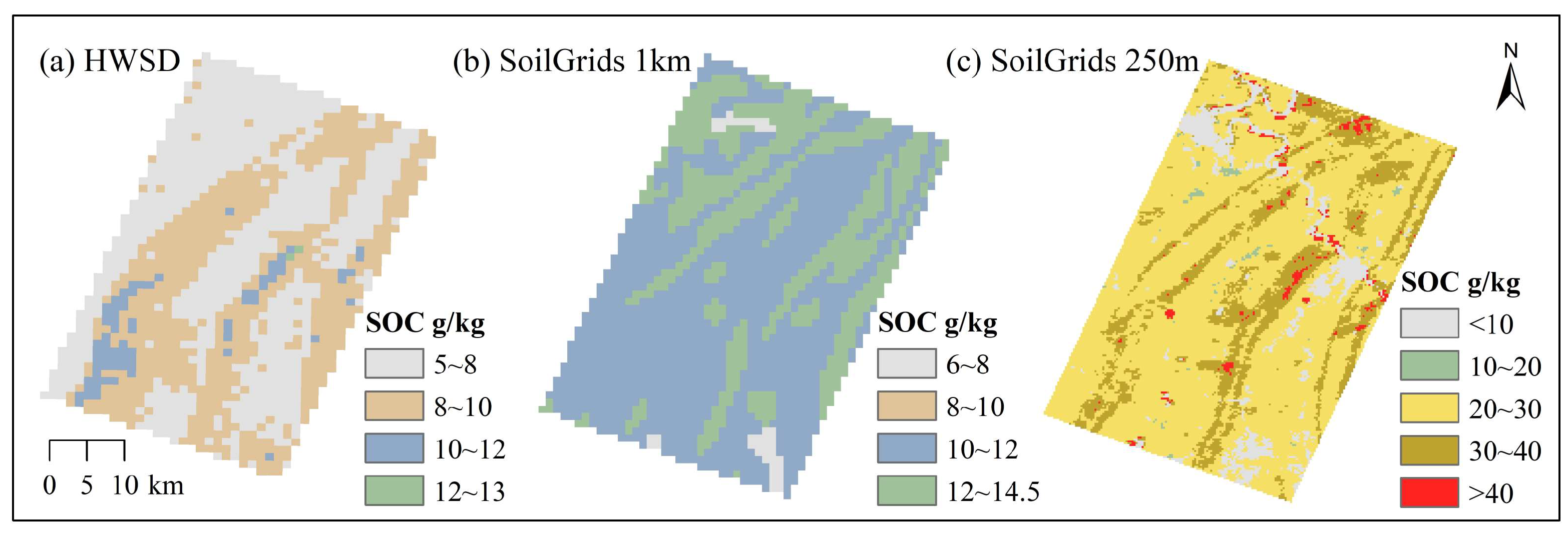
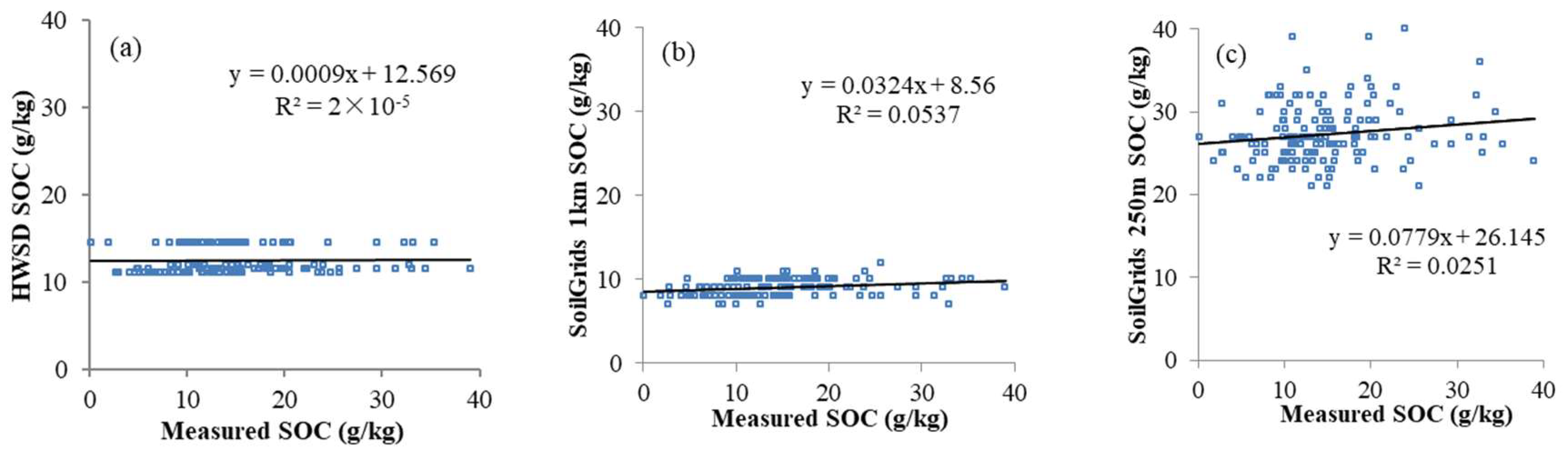
4.3. Comparison to Other Existing Products

The predicted map of SOC content was compared to those obtained with three other SOC products, including the SoilGrids with 1 km resolution [68], SoilGrids with 250 m resolution [28] and harmonized world soil database (HWSD) [69] (Figure 5). Generally, the carbon concentration of the SG250 m exhibited a similar trend to that of our predicted map in spatial distribution. On the contrary, the results of HWSD and SG1 km substantially differed from those of our map. In most study areas, the difference between our SOC predictions and those of SG250 m was significantly smaller than the difference between our predicted values and those predicted with HWSD or SG 1km. Here, the biggest difference was the range of the SOC predictions. Specifically, the HWSD and SG1km products seemed to underestimate the SOC content. These products also reported relatively low values in the forest where high SOC content was observed based on our field investigation. We also verified the SOC estimated values of these data products using our soil sampling data (Figure 6) and found a general overestimation of SOC content by the SG250m product. In contrast, both the HWSD and the SG1 km severely underestimated the SOC content. In the current study area, the topography is highly undulating and exhibits a high spatial heterogeneity. Therefore, global models such as SoilGrids are likely to be unsuitable for areas with a high spatial heterogeneity, and instead a local model would be more appropriate.

5. Conclusions

In this study, we generated a map detailing the spatial distribution of the predicted SOC levels in northwest Chongqing, China, by evaluating and comparing the SVM, RF and XGBoost models. In order to predict the SOC content of different types of land use, different driving factors were selected. Optical remote sensing bands and derived indices, precipitation and mean annual temperature were the main driving variables associated with the variation of SOC content in both the forest areas and the entire sampling area, while in the farmland area, they were optical remote sensing band11 and Pop-density. In contrast to previous studies, SAR remote sensing data were not applicable for predicting SOC content in karst areas. In predicting SOC content, the RF and XGBoost models showed superior performance and effectiveness compared to the SVM model. Meanwhile, for the forest and farmland, the RF and XGBoost algorithms showed a correspondingly better performance. The prediction model based on different land use types could obtain higher simulation accuracy than the model based on the whole study area. In the future, more field sampling and other remote sensing sensors should be considered as predictor variables for SOC content modeling.

Author Contributions

Conceptualization, W.Z.; Data curation, L.Y.; Formal analysis, J.X. and K.W.; Investigation, H.L.; Methodology, T.W. and W.Z.; Project administration, L.Y.; Resources, H.L. and K.W.; Software, T.W.; Supervision, W.Z.; Validation, J.X.; Visualization, L.X.; Writing—original draft, T.W.; Writing—review & editing, L.X. All authors have read and agreed to the published version of the manuscript.

Funding

This work and article processing charge were funded by the Project of Chongqing Science and Technology Bureau (cstc2021jcyj-msxmX0384), the Fundamental Research Funds for the Central Universities (SWU020015, SWU2209225), the National Natural Science Foundation of China (41930647, 41501575), the Strategic Priority Research Program (A) of the Chinese Academy of Sciences (XDA20030203), the Innovation Project of LREIS (O88RA600YA). We would like to thank the HighEdit company for assistance with English language editing of this manuscript.

Data Availability Statement

The data presented in this study are available on request from the corresponding author.

Conflicts of Interest

There is no conflict of interest for the authors of this article.

References

  1. Tifafi, M.; Guenet, B.; Hatté, C. Large Differences in Global and Regional Total Soil Carbon Stock Estimates Based on SoilGrids, HWSD, and NCSCD: Intercomparison and Evaluation Based on Field Data from USA, England, Wales, and France. Glob. Biogeochem. Cycle 2018, 321, 42–56. [Google Scholar] [CrossRef]
  2. Batjes, N.H. Total carbon and nitrogen in the soils of the world. Eur. J. Soil Sci. 1996, 47, 151–163. [Google Scholar] [CrossRef]
  3. Lal, R. Soil carbon sequestration to mitigate climate change. Geoderma 2004, 123, 1–22. [Google Scholar] [CrossRef]
  4. Conant, R.T.; Ogle, S.M.; Paul, E.A.; Paustian, K. Measuring and monitoring soil organic carbon stocks in agricultural lands for climate mitigation. Front. Ecol. Environ. 2011, 9, 169–173. [Google Scholar] [CrossRef]
  5. Lal, R. Soil Carbon Sequestration Impacts on Global Climate Change and Food Security. Science 2004, 304, 1623–1627. [Google Scholar] [CrossRef]
  6. Soussana, J.; Lutfalla, S.; Ehrhardt, F.; Rosenstock, T.; Lamanna, C.; Havlík, P.; Richards, M.; Wollenberg, E.L.; Chotte, J.; Torquebiau, E.; et al. Matching policy and science: Rationale for the ‘4 per 1000—Soils for food security and climate’ initiative. Soil Tillage Res. 2019, 188, 3–15. [Google Scholar] [CrossRef]
  7. Yang, L.; Luo, P.; Wen, L.; Li, D. Soil organic carbon accumulation during post-agricultural succession in a karst area, southwest China. Sci. Rep. 2016, 6, 37118. [Google Scholar] [CrossRef]
  8. Chen, S.; Saby, N.P.; Martin, M.P.; Barthès, B.G.; Gomez, C.; Shi, Z.; Arrouays, D. Integrating additional spectroscopically inferred soil data improves the accuracy of digital soil mapping. Geoderma 2023, 433, 116467. [Google Scholar] [CrossRef]
  9. Searle, R.; McBratney, A.; Grundy, M.; Kidd, D.; Malone, B.; Arrouays, D.; Stockman, U.; Zund, P.; Wilson, P.; Wilford, J. Digital soil mapping and assessment for Australia and beyond: A propitious future. Geoderma Reg. 2021, 24, e359. [Google Scholar] [CrossRef]
  10. Liu, F.; Wu, H.Y.; Zhao, Y.G.; Li, D.C.; Yang, J.L.; Song, X.D.; Shi, Z.; Zhu, A.X.; Zhang, G.L. Mapping high resolution National Soil Information Grids of China. Sci. Bull. 2021, 10, 1016. [Google Scholar] [CrossRef]
  11. Minasny, B.; McBratney Alex, B. Digital soil mapping: A brief history and some lessons. Geoderma 2016, 264, 301–311. [Google Scholar] [CrossRef]
  12. Zhou, T.; Geng, Y.; Chen, J.; Liu, M.; Lausch, A. Mapping soil organic carbon content using multi-source remote sensing variables in the Heihe River Basin in China. Ecol. Indic. 2020, 114, 1–10. [Google Scholar] [CrossRef]
  13. Chen, Y.; Ma, L.X.; Yu, D.S.; Zhang, H.D.; Feng, K.Y.; Wang, X.; Song, J. Comparison of feature selection methods for mapping soil organic matter in subtropical restored forests. Ecol. Indic. 2022, 135, 108545. [Google Scholar] [CrossRef]
  14. Taghizadeh-Mehrjardi, R.; Schmidt, K.; Amirian-Chakan, A.; Rentschler, T.; Zeraatpisheh, M.; Sarmadian, F.; Valavi, R.; Davatgar, N.; Behrens, T.; Scholten, T. Improving the Spatial Prediction of Soil Organic Carbon Content in Two Contrasting Climatic Regions by Stacking Machine Learning Models and Rescanning Covariate Space. Remote Sens. 2020, 12, 1095. [Google Scholar] [CrossRef]
  15. Emadi, M.; Taghizadeh-Mehrjardi, R.; Cherati, A.; Danesh, M.; Mosavi, A.; Scholten, T. Predicting and mapping of soil organic carbon using machine learning algorithms in Northern Iran. Remote Sens. 2020, 12, 2234. [Google Scholar] [CrossRef]
  16. Gomes, L.C.; Faria, R.M.; de Souza, E.; Veloso, G.V.; Schaefer, C.E.G.R.; Filho, E.I.F. Modelling and mapping soil organic carbon stocks in Brazil. Geoderma 2019, 340, 337–350. [Google Scholar] [CrossRef]
  17. Mishra, U.; Lal, R.; Liu, D.; Meirvenne, M.V. Predicting the Spatial Variation of the Soil Organic Carbon Pool at a Regional Scale. Soil Sci. Soc. Am. J. 2010, 74, 906–914. [Google Scholar] [CrossRef]
  18. Ottoy, S.; Vos, B.D.; Sindayihebura, A.; Hermy, M.; Orshoven, J.V. Assessing soil organic carbon stocks under current and potential forest cover using digital soil mapping and spatial generalisation. Ecol. Indic. 2017, 77, 139–150. [Google Scholar]
  19. Ballabio, C.; Fava, F.; Rosenmund, A. A plant ecology approach to digital soil mapping, improving the prediction of soil organic carbon content in alpine grasslands. Geoderma 2012, 187, 102–116. [Google Scholar] [CrossRef]
  20. Grinand, C.; Maire, G.L.; Vieilledent, G.; Razakamanarivo, H.; Razafimbelo, T.; Bernoux, M. Estimating temporal changes in soil carbon stocks at ecoregional scale in Madagascar using remote-sensing. Int. J. Appl. Earth Obs. Geoinf. 2017, 54, 1–14. [Google Scholar] [CrossRef]
  21. Wang, Y.; Deng, L.; Wu, G.; Wang, K.; Shangguan, Z. Large-scale soil organic carbon mapping based on multivariate modelling: The case of grasslands on the Loess Plateau. Land Degrad. Dev. 2018, 29, 26–37. [Google Scholar] [CrossRef]
  22. Garnier, J.; Billen, G.; Tournebize, J.; Barre, P.; Mary, B.; Baudin, F. Storage or loss of soil active carbon in cropland soils: The effect of agricultural practices and hydrology. Geoderma 2022, 407, 115538. [Google Scholar]
  23. Li, J.Y.; Zhang, D.Y.; Liu, M. Factors controlling the spatial distribution of soil organic carbon in Daxing’anling Mountain. Sci. Rep. 2020, 10, 1–8. [Google Scholar] [CrossRef] [PubMed]
  24. Demattê, J.; Sayo, V.M.; Rizzo, R.; Fongaro, C.T. Soil class and attribute dynamics and their relationship with natural vegetation based on satellite remote sensing. Geoderma 2017, 302, 39–51. [Google Scholar] [CrossRef]
  25. Zhou, Y.; Chen, S.C.; Zhu, A.X.; Hu, B.F.; Li, Y. Revealing the scale- and location-specific controlling factors of soil organic carbon in Tibet. Geoderma 2021, 382, 114713. [Google Scholar] [CrossRef]
  26. Poggio, L.; Gimona, A. Assimilation of optical and radar remote sensing data in 3D mapping of soil properties over large areas. Sci. Total Environ. 2017, 579, 1094–1110. [Google Scholar] [CrossRef]
  27. Yang, R.M.; Guo, W.W. Using time-series Sentinel-1 data for soil prediction on invaded coastal wetlands. Environ. Monit. Assess. 2019, 191, 462. [Google Scholar] [CrossRef]
  28. Hengl, T.; Mendes De Jesus, J.; Heuvelink, G.B.M.; Ruiperez Gonzalez, M.; Kilibarda, M.; Blagotić, A.; Shangguan, W.; Wright, M.N.; Geng, X.; Bauer-Marschallinger, B.; et al. SoilGrids250m: Global gridded soil information based on machine learning. PLoS ONE 2017, 12, e169748. [Google Scholar] [CrossRef]
  29. Jiang, Z.C.; Lian, Y.Q.; Qin, X.Q. Rocky desertification in Southwest China: Impacts, causes, and restoration. Earth-Sci. Rev. 2014, 132, 1–12. [Google Scholar] [CrossRef]
  30. Dong, G.; Fan, L.; Fensholt, R.; Frappart, F.; Ciais, P.; Xiao, X.; Sitch, S.; Xing, Z.; Yu, L.; Zhou, Z. Asymmetric response of primary productivity to precipitation anomalies in Southwest China. Agric. For. Meteorol. 2023, 331, 109350. [Google Scholar] [CrossRef]
  31. Zhang, E.Q.; Zhang, H.Q. Characterization and interaction of driving factors in karst rocky desertification: A case study from Changshun, China. Solid Earth 2014, 5, 1329–1340. [Google Scholar]
  32. Yan, H.; Cao, M.; Liu, J.; Tao, B. Potential and sustainability for carbon sequestration with improved soil management in agricultural soils of China. Agric. Ecosyst. Environ. 2007, 121, 325–335. [Google Scholar] [CrossRef]
  33. Yu, G.; Li, X.; Wang, Q.; Li, S. Carbon storage and its spatial pattern of terrestrial ecosystem in China. J. Resour. Ecol. 2010, 1, 97–109. [Google Scholar]
  34. Zhang, Z.; Zhou, Y.; Wang, S.; Huang, X. Patterns and influencing factors of spatio-temporal variability of soil organic carbon in karst catchment. Int. J. Glob. Warm. 2019, 17, 89–107. [Google Scholar] [CrossRef]
  35. Zanaga, D.; Van De Kerchove, R.; De Keersmaecker, W.; Souverijns, N.; Brockmann, C.; Quast, R.; Wevers, J.; Grosu, A.; Paccini, A.; Vergnaud, S. ESA WorldCover 10 m 2020 v100. 2021. Available online: https://viewer.esa-worldcover.org/worldcover/ (accessed on 1 March 2022).
  36. Laurencelle, J.; Logan, T.; Gens, R. ASF radiometrically terrain corrected ALOS PALSAR products. ASF-Alaska Satell. Facil. 2015, 1, 12. [Google Scholar]
  37. Socioeconomic, D.A.A.C. Gridded Population of the World (GPW), v4. 2005. Available online: https://sedac.ciesin.columbia.edu/data/set/gpw-v4-population-density-rev11 (accessed on 5 March 2022).
  38. Elhag, M.; Bahrawi, J.A. Soil salinity mapping and hydrological drought indices assessment in arid environments based on remote sensing techniques. Geosci. Instrum. Methods Data Syst. 2017, 6, 149–158. [Google Scholar] [CrossRef]
  39. Maynard, J.J.; Levi, M.R. Hyper-temporal remote sensing for digital soil mapping: Characterizing soil-vegetation response to climatic variability. Geoderma 2017, 285, 94–109. [Google Scholar] [CrossRef]
  40. Jin, X.; Du, J.; Liu, H.; Wang, Z.; Song, K. Remote estimation of soil organic matter content in the Sanjiang Plain, Northest China: The optimal band algorithm versus the GRA-ANN model. Agric. For. Meteorol. 2016, 218, 250–260. [Google Scholar] [CrossRef]
  41. Jin, X.; Song, K.; Du, J.; Liu, H.; Wen, Z. Comparison of different satellite bands and vegetation indices for estimation of soil organic matter based on simulated spectral configuration. Agric. For. Meteorol. 2017, 244, 57–71. [Google Scholar] [CrossRef]
  42. Liu, S.; An, N.; Yang, J.; Dong, S.; Wang, C.; Yin, Y. Prediction of soil organic matter variability associated with different land use types in mountainous landscape in southwestern Yunnan province, China. Catena 2015, 133, 137–144. [Google Scholar] [CrossRef]
  43. Drusch, M.; Del Bello, U.; Carlier, S.; Colin, O.; Fernandez, V.; Gascon, F.; Hoersch, B.; Isola, C.; Laberinti, P.; Martimort, P.; et al. Sentinel-2: ESA’s Optical High-Resolution Mission for GMES Operational Services. Remote Sens. Environ. 2012, 120, 25–36. [Google Scholar] [CrossRef]
  44. Escadafal, R. Remote sensing of arid soil surface color with Landsat thematic mapper. Adv. Space Res. 1989, 9, 159–163. [Google Scholar] [CrossRef]
  45. Pouget, M.; Madeira, J.; Le Floc H, E.; Kamal, S. Caracteristiques spectrales des surfaces sableuses de la region cotiere nord-ouest de l’Egypte: Application aux donnees satellitaires SPOT. Proc. 2e’me Journées Télédétection. In Caractérisation et Suivi des Milieux Terrestres en Régions Arides et Tropicales; ORSTOM: Bondy, Japan, 1991; pp. 27–38. [Google Scholar]
  46. Hengl, T. A Practical Guide to Geostatistical Mapping; Office for Official Publications of the European Communities: Luxembourg, 2009. [Google Scholar]
  47. Gitelson, A.A.; Kaufman, Y.J.; Merzlyak, M.N. Use of a green channel in remote sensing of global vegetation from EOS-MODIS. Remote Sens. Environ. 1996, 58, 289–298. [Google Scholar] [CrossRef]
  48. Rouse, J.W.; Haas, R.H.; Schell, J.A.; Deering, D.W. Monitoring vegetation systems in the great plains with ERTS. NASA Spec. Publ. 1974, 351, 309. [Google Scholar]
  49. Huete, A.R. A soil-adjusted vegetation index (SAVI). Remote Sens. Environ. 1988, 25, 295–309. [Google Scholar] [CrossRef]
  50. Nellis, M.D.; Briggs, J.M. Transformed vegetation index for measuring spatial variation in drought impacted biomass on Konza Prairie, Kansas. Trans. Kans. Acad. Sci. 1992, 95, 93–99. [Google Scholar] [CrossRef]
  51. Vapnik, V. The Nature of Statistical Learning Theory; Springer Science & Business Media: Berlin/Heidelberg, Germany, 1999. [Google Scholar]
  52. Elith, J.; Leathwick, J.R.; Hastie, T. A working guide to boosted regression trees. J. Anim. Ecol. 2008, 77, 802–813. [Google Scholar] [CrossRef]
  53. Dieleman, W.I.; Venter, M.; Ramachandra, A.; Krockenberger, A.K.; Bird, M.I. Soil carbon stocks vary predictably with altitude in tropical forests: Implications for soil carbon storage. Geoderma 2013, 204, 59–67. [Google Scholar] [CrossRef]
  54. Girardin, C.A.J.; Malhi, Y.; Aragao, L.; Mamani, M.; Huaraca Huasco, W.; Durand, L.; Feeley, K.J.; Rapp, J.; Silva Espejo, J.E.; Silman, M. Net primary productivity allocation and cycling of carbon along a tropical forest elevational transect in the Peruvian Andes. Glob. Change Biol. 2010, 16, 3176–3192. [Google Scholar] [CrossRef]
  55. Wang, B.; Waters, C.; Orgill, S.; Gray, J.; Cowie, A.; Clark, A.; Li Liu, D. High resolution mapping of soil organic carbon stocks using remote sensing variables in the semi-arid rangelands of eastern Australia. Sci. Total Environ. 2018, 630, 367–378. [Google Scholar] [CrossRef]
  56. Zhou, T.; Geng, Y.; Chen, J.; Sun, C.; Lausch, A. Mapping of Soil Total Nitrogen Content in the Middle Reaches of the Heihe River Basin in China Using Multi-Source Remote Sensing-Derived Variables. Remote Sens. 2019, 11, 2934. [Google Scholar] [CrossRef]
  57. Wang, S.; Jin, X.; Adhikari, K.; Li, W.; Yu, M.; Bian, Z.; Wang, Q. Mapping total soil nitrogen from a site in northeastern China. Catena 2018, 166, 134–146. [Google Scholar] [CrossRef]
  58. Ceddia, M.B.; Gomes, A.S.; Vasques, G.M.; Pinheiro, E.F.M. Soil Carbon Stock and Particle Size Fractions in the Central Amazon Predicted from Remotely Sensed Relief, Multispectral and Radar Data. Remote Sens. 2017, 9, 124. [Google Scholar] [CrossRef]
  59. Bouman, B.A.; Hoekman, D.H. Multi-temporal, multi-frequency radar measurements of agricultural crops during the Agriscatt-88 campaign in The Netherlands. Titleremote Sens. 1993, 14, 1595–1614. [Google Scholar] [CrossRef]
  60. Hajnsek, I.; Jagdhuber, T.; Schon, H.; Papathanassiou, K.P. Potential of estimating soil moisture under vegetation cover by means of PolSAR. IEEE Trans. Geosci. Remote Sens. 2009, 47, 442–454. [Google Scholar] [CrossRef]
  61. Burgin, M.; Clewley, D.; Lucas, R.M.; Moghaddam, M. A generalized radar backscattering model based on wave theory for multilayer multispecies vegetation. IEEE Trans. Geosci. Remote Sens. 2011, 49, 4832–4845. [Google Scholar] [CrossRef]
  62. Thompson, J.A.; Kolka, R.K. Soil Carbon Storage Estimation in a Forested Watershed Using Quantitative Soil-Landscape Modeling. Soil Sci. Soc. Am. J. 2005, 69, 1086–1093. [Google Scholar] [CrossRef]
  63. Tomislav, H.; Jorge, M.D.J.; Heuvelink, G.B.M.; Maria, R.G.; Milan, K.; Aleksandar, B.; Wei, S.; Wright, M.N.; Xiaoyuan, G.; Bernhard, B.M. Soil Grids 250m: Global gridded soil information based on machine learning. PLoS ONE 2017, 12, e169748. [Google Scholar]
  64. Wang, S.; Zhuang, Q.; Wang, Q.; Jin, X.; Han, C. Mapping stocks of soil organic carbon and soil total nitrogen in Liaoning Province of China. Geoderma 2017, 305, 250–263. [Google Scholar] [CrossRef]
  65. Tsui, C.C.; Tsai, C.C.; Chen, Z.S. Soil organic carbon stocks in relation to elevation gradients in volcanic ash soils of Taiwan. Geoderma 2013, 209, 119–127. [Google Scholar] [CrossRef]
  66. Obu, J.; Lantuit, H.; Myers-Smith, I.; Heim, B.; Wolter, J.; Fritz, M. Effect of Terrain Characteristics on Soil Organic Carbon and Total Nitrogen Stocks in Soils of Herschel Island, Western Canadian Arctic. Permafr. Periglac. Process. 2017, 28, 92–107. [Google Scholar] [CrossRef]
  67. Schuur, E.A.G.; McGuire, A.D.; Schaedel, C.; Grosse, G.; Harden, J.W.; Hayes, D.J.; Hugelius, G.; Koven, C.D.; Kuhry, P.; Lawrence, D.M.; et al. Climate change and the permafrost carbon feedback. Nature 2015, 520, 171–179. [Google Scholar] [CrossRef] [PubMed]
  68. Hengl, T.; de Jesus, J.M.; MacMillan, R.A.; Batjes, N.H.; Heuvelink, G.B.; Ribeiro, E.; Samuel-Rosa, A.; Kempen, B.; Leenaars, J.G.; Walsh, M.G. SoilGrids1km—Global soil information based on automated mapping. PLoS ONE 2014, 9, e105992. [Google Scholar] [CrossRef] [PubMed]
  69. FAO. Harmonized World Soil Database, version 1.2; FAO: Rome, Italy; IIASA: Laxenburg, Austria, 2012. [Google Scholar]
Figure 1. Spatial location of the study area (a,b), land use/land cover map (c) and spatial distribution of the sampling points (d) in the study area.
Remotesensing 15 02118 g001
Figure 2. Correlation matrices between SOC and corresponding variables for the overall (a), forest (b) and farmland areas (c). ** correlation is significant at the 0.01 level, * correlation is significant at the 0.05 level.
Remotesensing 15 02118 g002aRemotesensing 15 02118 g002b
Figure 3. Comparison of the variables in terms of their relative importance using the RF model for the overall study area (left), forest area (middle) and farmland (right).
Remotesensing 15 02118 g003
Figure 4. SOC content mapping based on the RF and XGBoost models.
Remotesensing 15 02118 g004
Figure 5. SOC content map by HWSD (a), SoilGrids 1 km (b) and SoilGrids 250 m (c).
Remotesensing 15 02118 g005
Figure 6. Validation of the measured SOC with (a) HWSD, (b) SG1k m and (c) SG250m.
Remotesensing 15 02118 g006
Table 1. Derived indices.
IndexDefinitionReference
BI ( ρ R e d × ρ R e d ) + ( ρ G r e e n × ρ G r e e n ) 2 [44]
BI2 ( ρ R e d × ρ R e d ) + ( ρ G r e e n × ρ G r e e n ) + ( ρ N I R × ρ N I R ) 3 [44]
CI ρ R e d ρ G r e e n ρ R e d + ρ G r e e n [45]
CI1 S W I R 1 S W I R 2 [46]
GNDVI ρ N I R ρ G r e e n ρ N I R + ρ G r e e n [47]
NDVI ρ N I R ρ R e d ρ N I R + ρ R e d [48]
SAVI ( ρ N I R ρ R e d ) × 1.5 ρ N I R ρ R e d + 0.5 [49]
TVI ρ N I R ρ R e d ρ N I R + ρ R e d + 0.5 × 100 [50]
Table 2. Technical specifications of Sentinel-2A bands used in this study.
BandSpectral Range (nm)Spectral Position
(nm)
WavelengthBand Width
(nm)
Spatial Resolution
(m)
B2458–523490Blue6510
B3543–578560Green3510
B4650–680665Red3010
B5698–713705Red Edg 11520
B8785–900842NIR11510
B111565–16551610SWIR 19020
B122100–22802190SWIR 218020
Table 3. Parameters of the Sentinel-1A data.
DateBeamPolarizationDirectionSpatial Resolution
(m)
18 January 2020IWVVDescending10
18 January 2020IWVHDescending10
Table 4. SOC content statistics for farmland and forest.
Sample TypeMinimum (g/kg)Maximum (g/kg)Average (g/kg)Standard DeviationKurtosisSkewnessCoefficient of Variation (%)
Overall0.1263.6616.039.926.262.1261.88
Forest0.1263.6618.1511.483.771.7863.25
Farmland1.8927.4312.685.300.570.4741.80
Table 5. SOC content statistics for different soil depths.
Soil depth
(cm)
Minimum (g/kg)Maximum (g/kg)Average (g/kg)Standard deviationKurtosisSkewnessCoefficient of Variation (%)
0~102.9767.1416.3210.066.52.0161.64
10~200.8253.9613.38.345.992.0262.71
20~300.6657.9211.957.9312.282.7766.36
Table 6. SOC prediction accuracy using different simulation models for different land use types.
Sample TypeModelsVerification
RMSER2MAE
OverallSVM8.150.129.56
RF7.350.175.74
XGBoost7.830.145.99
ForestSVM12.460.1110.58
RF6.810.325.63
XGBoost8.810.256.86
FarmlandSVM5.80.155.01
RF4.140.233.40
XGBoost4.030.283.27
Table 7. Descriptive statistics of predicted SOC content using the RF and XGBoost models for forest and farmland.
Sample TypeMinimum
(g/kg)
Maximum
(g/kg)
Average
(g/kg)
Standard Deviation
Forest11.2839.5321.855.64
Farmland2.9925.8111.543.69
Disclaimer/Publisher’s Note: The statements, opinions and data contained in all publications are solely those of the individual author(s) and contributor(s) and not of MDPI and/or the editor(s). MDPI and/or the editor(s) disclaim responsibility for any injury to people or property resulting from any ideas, methods, instructions or products referred to in the content.

