Article

Automation in Middle- and Upper-Atmosphere LIDAR Operations: A Maximum Rayleigh Altitude Prediction System Based on Night Sky Imagery

1
Hubei Key Laboratory of Intelligent Wireless Communications, College of Electronics and Information Engineering, South-Central Minzu University, Wuhan 430074, China
2
Innovation Academy for Precision Measurement Science and Technology, Chinese Academy of Sciences, Wuhan 430071, China
3
Wuhan TopStar Optronics Technology Co., Ltd., Wuhan 430071, China
4
State Key Laboratory of Space Weather, National Space Science Center, Chinese Academy of Sciences, Beijing 100190, China
5
College of Computer Science, South-Central Minzu University, Wuhan 430074, China
*
Author to whom correspondence should be addressed.
Remote Sens. 2024, 16(3), 536; https://doi.org/10.3390/rs16030536
Submission received: 8 November 2023 / Revised: 24 January 2024 / Accepted: 24 January 2024 / Published: 31 January 2024
(This article belongs to the Section Atmospheric Remote Sensing)

Abstract

:
A prediction system was developed to determine the maximum Rayleigh altitude (MRA) by improving the automated detection of LIDAR power-on conditions and adapting to advancements in middle- and upper-atmosphere LIDAR technology. The proposed system was developed using observational data and nighttime sky imagery collected from multiple LIDAR stations. To assess the accuracy of predictions, three key parameters were employed: mean square error, root mean square error, and mean absolute error. Among the three prediction models created through multivariate regression and autoregressive integrated moving average (ARIMA) analyses, the most suitable model was selected for predicting the MRA. One-month predictions demonstrated the accuracy of the MRA with a maximum error of no more than 5 km and an average error of less than 2 km. This technology has been successfully implemented in numerous LIDAR stations, enhancing their automation capabilities and providing key technical support for large-scale, unmanned, and operational deployments in the middle- and upper-atmosphere LIDAR systems.

1. Introduction

The middle- and upper-atmosphere LIDAR (MUA-LIDAR) is a crucial optical and electronic device utilized to detect atmospheric activity at altitudes ranging from 30 to 300 km above the Earth’s surface [1]. It plays a pivotal role in research related to the evolution of metallic layers, the interaction of neutral and ionized components, atmospheric fluctuation propagation, and nonlinear interactions [2,3,4,5]. Numerous MUA-LIDAR stations have been established worldwide, including in China, forming a significant observation network [6].
While these established MUA-LIDAR stations excel in hardware performance and detection capabilities for various scientific endeavors, they still heavily rely on manual management, maintenance, and operation, lacking the desired level of automation [7]. Among the numerous factors impeding the further advancement of MUA-LIDAR technology, the automatic identification of weather conditions has become an important bottleneck. Existing weather forecasting techniques, whether derived from surface-based meteorological observation stations or satellite cloud maps, fall short in terms of location accuracy and timeliness [8]. MUA-LIDAR operations are highly weather-dependent, with optimal observations attainable only in clear weather [9]. In adverse weather conditions (e.g., cloud cover, fog, or haze), MUA-LIDAR can only capture echo signals below 35 km, which is insignificant for the inversion of crucial MUA parameters like temperature, density, and wind fields. Consequently, these types of LIDAR data have limited research value for theoretical MUA studies. Moreover, sudden localized wind gusts or minor precipitation can severely damage the equipment, jeopardizing the safe operation of the MUA-LIDAR system. Existing weather forecasting techniques cannot provide precise weather predictions 5 to 10 min immediately ahead in LIDAR stations. At present, China offers national weather forecasts with a resolution of 5 km and hourly updates [10]. The United States’ National Digital Forecast Database (NDFD) can provide continuous gridded weather forecasts at resolutions of 2.5/5 km with hourly updates [11]. The Austrian National Weather Service delivers probabilistic and deterministic weather forecasts updated every 10 min with a minimum resolution of 1 km [12]. The Deutscher Wetterdienst (DWD) furnishes weather forecasts updated every 5 min at 2.5 km resolution by leveraging robust numerical modeling capabilities [13]. In practice, most existing or planned Chinese LIDAR stations are situated far from meteorological observation stations. A representative example is the Yuzhong station (104.13°E, 35.95°N) of the Lanzhou station, which is located on the Loess Plateau at an elevation of nearly 2 km, more than 47 km away from the Yuzhong meteorological station (104.09°E, 35.52°N), which is often subject to cloudy and foggy weather [14]. As is the case there, the assessment of weather conditions at most LIDAR stations relies on subjective predictions by experienced personnel based on current local weather conditions.
The reliance on subjective weather predictions often leads to issues with the operation of MUA-LIDAR systems. Weather condition standards are typically set conservatively for the safety of the equipment, resulting in severely limited operating hours. For example, the Beijing Yanqing station (115.97°E, 40.45°N) had fewer than 140 days of observations in the entire year of 2022, with a total observation time of approximately 1348 h. However, relaxing these standards to increase observation hours significantly raises the risk of damaging equipment. Adopting less stringent standards can also yield copious data of limited research significance, effectively wasting the lifespan of the laser. Ensuring data validity and equipment safety necessitates a constant watch on outdoor weather conditions, proactive warnings about potential severe weather, and the adoption of appropriate measures to protect equipment and secure high-value data—a task that cannot be efficiently handled by human personnel.
Determining the appropriate weather condition standard, as mentioned above, has become a major obstacle in the operation and intelligent management of today’s MUA-LIDAR stations. Given the substantial operational costs associated with these LIDAR systems, lenient standards can result in an excess of low-quality and low-value data, while overly stringent standards can yield insufficient data. Furthermore, manual prediction standards are subjective and heavily rely on personnel expertise, hindering the standardization and automation of MUA-LIDAR operations. This paper introduces the maximum Rayleigh altitude (MRA) as a benchmark for evaluating the quality of LIDAR data. It establishes whether the MUA-LIDAR systems operate at altitudes greater than 35 km as the threshold for operations, thus achieving the automatic identification of MUA-LIDAR operational conditions.

2. Methods

2.1. Maximum Rayleigh Altitude

The MRA characterizes the uppermost altitude at which MUA-LIDAR can detect Rayleigh echo signals over the Earth’s atmosphere. Several factors influence the altitude of the Rayleigh echo, including weather conditions, the LIDAR power, the telescope receiving area, and the status of the transmitter–receiver. When MUA-LIDAR parameters remain constant, the MRA is predominantly influenced by low-altitude weather conditions since laser emissions and high-altitude raw echo optical signals traverse the lower atmosphere twice. Previous research has indicated that a higher MRA enhances the detection of metal layers in the middle and upper atmosphere [15]. In addition, the MRA can be conveniently inferred from metal-layer LIDAR data by simply excluding data at higher altitudes, making it an important evaluation index for the operational status of the metal-layer LIDAR system [16].
Typically, the MRA is inferred based on the signal-to-noise ratio of the photon-counted raw echo signal [17]. The laser’s atmospheric backscatter signal is weak, rendering it susceptible to noise interference and leading to significant errors in MRA calculation. Thus, it is imperative to process echo signals when utilizing the photon counting method to minimize errors.
As illustrated in Equation (1), the signal-to-noise (SNR) ratio is computed as the ratio of the photon counts in echo signals (S) to the photons originating from the background noise. S = N s i g N B a c k g r o u n d , where N s i g represents the number of photons corresponding to the detected altitude band, and N B a c k g r o u n d represents the number of photons present in the background altitude band. Both N s i g and N B a c k g r o u n d can be directly retrieved from the LIDAR echo signal. When employing the photon counting method, the noise distribution is represented by a Poisson distribution with N o i s e = N s i g .
S N R = S N o i s e
In our MRA calculation, we defined the effective detection range by setting the altitude area with an SNR ratio exceeding 3 [18,19]. In this setup, the signal strength is significantly higher than the noise level, resulting in lower variability in measurement results that can be replicated under different experimental conditions. The collected data were subjected to filtering, denoising, moving averages, and downsampling operations. We applied the SNR formula to minimize data noise. Subsequently, we used the Savitzky–Golay filter, which is based on local polynomial least-square fitting in the time domain. It is widely used for data stream smoothing and denoising, as it filters out noise while ensuring that the shape and width of the signal remain unchanged [20]. A moving average operation was then performed on the acquired data by selecting 12 consecutive data points and averaging them after removing the maximum and minimum values [21]. The moving average operation reduces the influence of individual data points, smooths irregular fluctuations in the data, and stably eliminates the influence of outliers on calculation results. The data collection system generated roughly two data points per minute. Downsampling was employed to reduce the data volume and optimize computational efficiency. This processing sequence minimized noise interference on the MRA calculations.
As shown in Figure 1, a large volume of MUA-LIDAR echo-signal data collected for each station was processed with this algorithm.
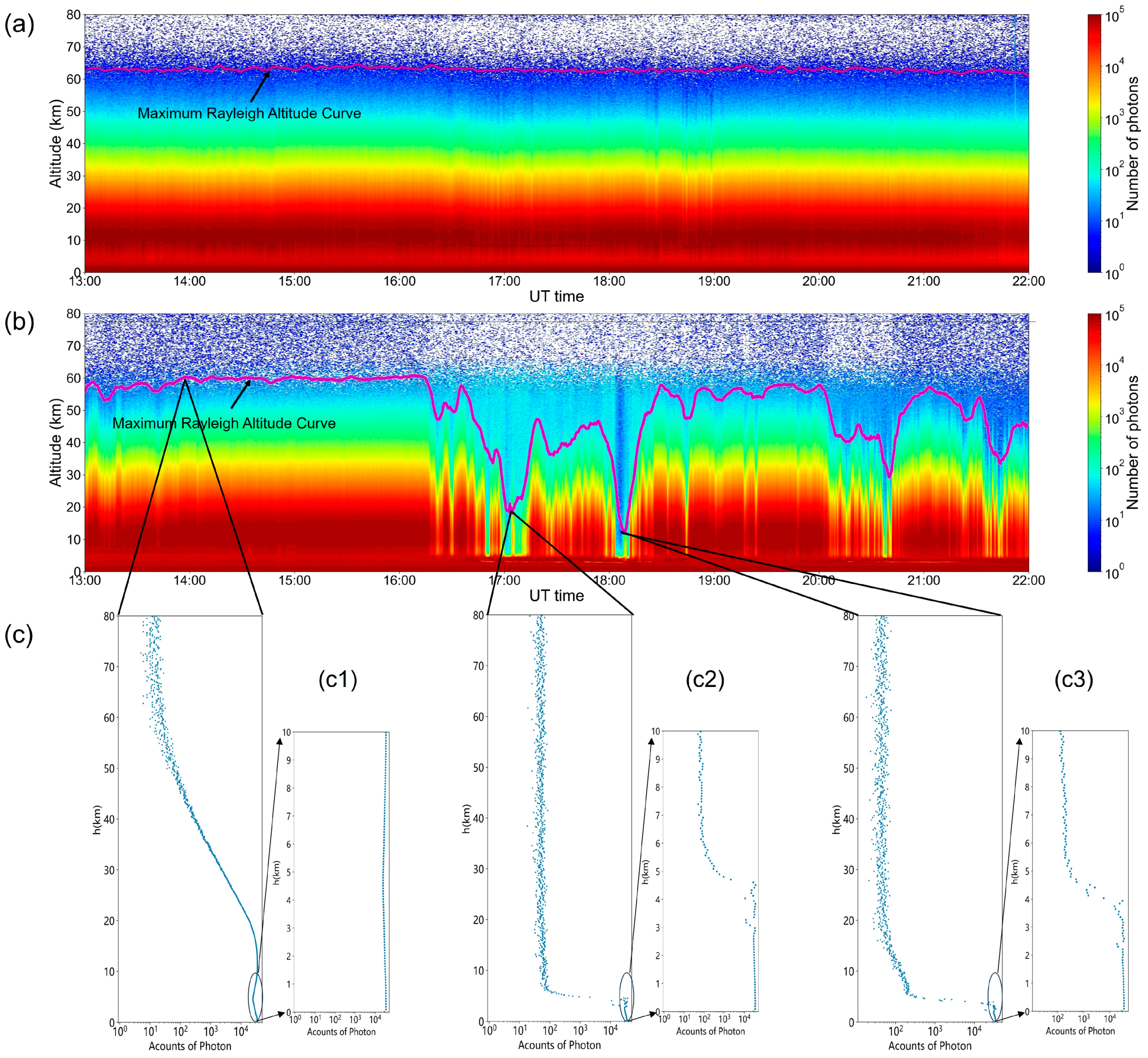
Figure 1a,b illustrate trends in the photon counts of echo signals and the MRA at the Beijing Yanqing station on the nights of 8 January 2023 and 16 January 2023, respectively. The MRA cases under fair night weather conditions and partly cloudy weather conditions were selected for further analysis. Fair weather conditions prevailed during the January 16 observation, leaving the MUA-LIDAR observations unaffected. Consequently, both the echo-signal photon counts and the MRA remained stable throughout the night without significant fluctuations. This situation is favorable for inverting the temperature, wind speed, and other related parameters in the MUA. Conversely, during the January 8 observation, the MRA of the MUA-LIDAR system significantly fluctuated for a portion of the night due to interference caused by cloudy weather. Lower altitude and more fluctuating MRA data are not conducive to scientific research. Figure 1c provides a specific example of the photon counts of echo signals versus detection altitude for a single time point shown in Figure 1b. Specifically, the weather conditions at the moment captured in Figure 1(c1) were fair, and the echo-signal photon counts were unaffected. The MRA reached 63,014 m. The adverse effect of cloudy weather on the MRA is evident in Figure 1(c2), with the photon counts of echo signals peaking at 4512 m, indicative of interference due to cloud cover approximately 288 m thick. At this time, the MRA was only 20,985 m. The moment shown in Figure 1(c3) was also impacted by cloudy weather, as the photon counts of echo signals peaked at 3936 m, indicating the cloud interference with a cloud thickness of about 288 m, resulting in an MRA of merely 15,331 m.
To summarize, weather exerts a significant impact on the MRA of MUA-LIDAR systems. The MRA serves as a critical indicator, reflecting current weather conditions, LIDAR power, and the matching status of the transmitter–receiver. Employing the proposed methodology for MRA calculations, we found that, under clear weather conditions and a constant laser state, the MRA remained generally stable throughout the night, with peak-to-peak fluctuations of less than 2 km within short intervals (30 min). When weather conditions change, the MRA value changes, demonstrating a high level of real-time sensitivity. This enables an accurate assessment of the MRA status of the MUA-LIDAR system.

2.2. Characteristics of Night Sky Images

Typically, MUA-LIDAR systems employ high-power lasers and large-aperture telescopes to capture faint echo light signals from the MUA. However, MUA-LIDAR systems do not function properly under adverse weather conditions such as rain, snow, strong winds, or dust storms. The intensity of rain and snow is typically measured by the amount of precipitation per unit of time. Strong winds are defined by a force greater than 5 on the Beaufort scale. Dust and floating weather can be evaluated based on the air quality index, which takes into account the contents of atmospheric particulate matter with a diameter equal to or below 10 microns, humidity, and wind speed [22,23]. Even in clear or partly cloudy weather, aerosols and haze are significant factors impairing these systems’ ability to detect the MUA. Clear weather is defined as a percentage of clouds between 0% and 10%, while partly cloudy weather is defined as having a percentage of clouds between 10% and 30% [
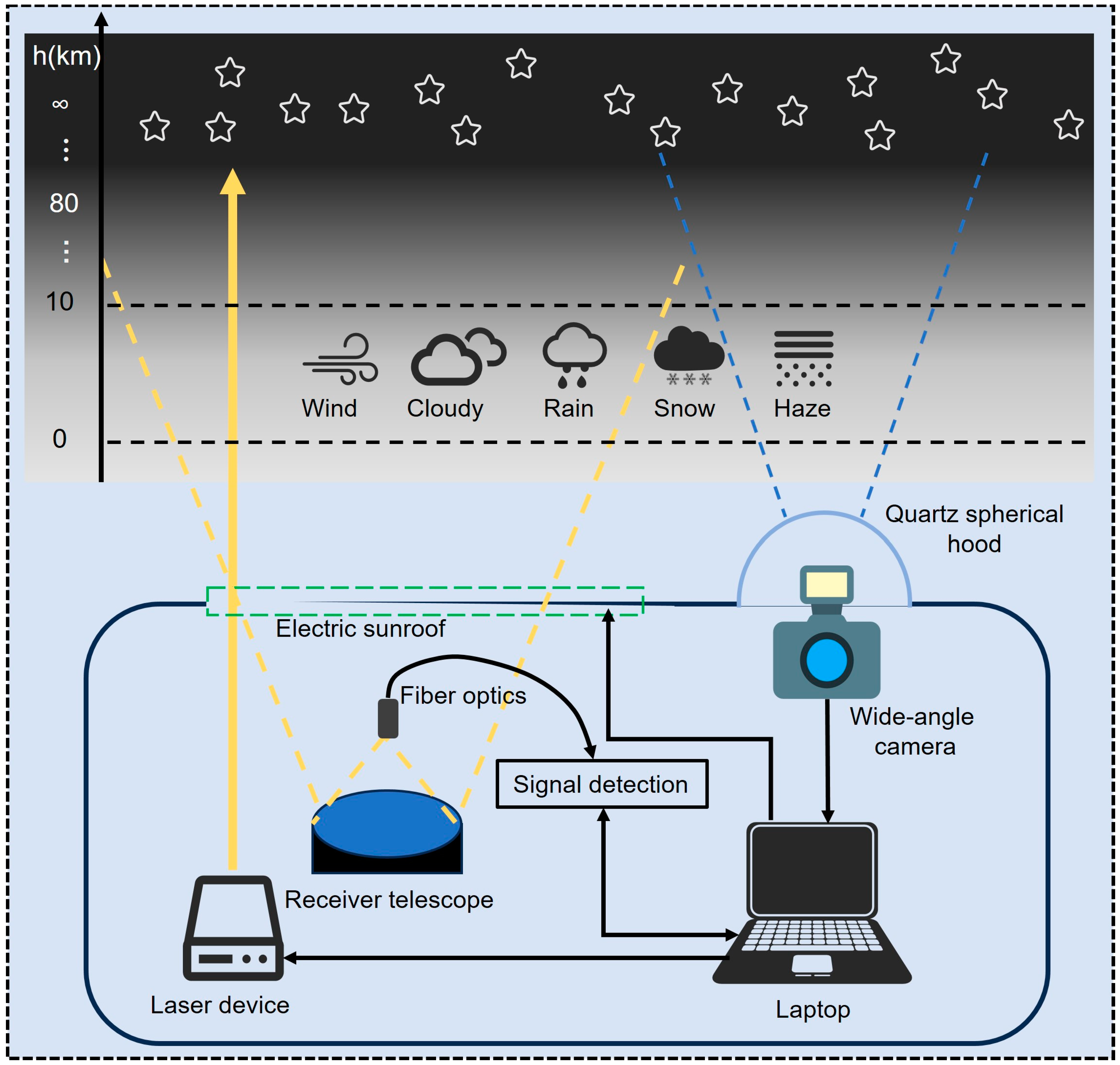
24]. These atmospheric elements, along with other factors near the LIDAR station, reduce the laser energy emitted, generate substantial background optical noise, and considerably attenuate the already faint echo light signals from the MUA. This further weakens the echo signals received by the telescope, directly impacting the optical transmittance of the LIDAR system and diminishing its capacity to monitor upper atmospheric conditions. Obtaining real-time weather information at LIDAR stations presents a formidable challenge that must be addressed in order to effectively utilize MUA-LIDAR technology. As depicted in Figure 2, the 0–10 km low-altitude range predominantly corresponds to a weather region that produces clouds, haze, high winds, and precipitation including rain and snow. These atmospheric conditions exert a significant impact on the safety and operational efficiency of MUA-LIDAR systems [25,26].
Above 10 km from the surface, the numerous stars in the distant Milky Way are highly stable, with minimal fluctuations in luminosity over brief time periods. Astronomers can assign static brightness classifications to each star. The twinkling effect observed in stars from the Earth’s surface is a result of various atmospheric factors that affect their luminosity, including turbulence, clouds, and aerosols. On clear, cloudless nights, atmospheric aerosols and haze scatter and absorb starlight to a lesser extent, resulting in brighter and more easily observed stars. In contrast, cloudy or adverse conditions (including the presence of aerosols and haze) lead to increased atmospheric scattering and absorption. Starlight weakens, causing stars to appear distorted or even disappear altogether from view. This reduces the number of observable stars and their overall brightness. Based on this principle, an astronomical camera can be installed at the LIDAR station to capture the distribution of stars, extract data for the number of stars and their brightness, and subsequently compare these data with star charts to ascertain local weather conditions. By predicting the MRA of the MUA-LIDAR system, it becomes possible to objectively assess the impact of environmental weather on the LIDAR’s observation capabilities. This facilitates the real-time monitoring and forecasting of the MRA and weather conditions, providing a valuable means of analyzing MUA-LIDAR performance.
During MUA-LIDAR observation, scattered light primarily originates from the 0–60 km range, fluorescence predominantly emanates from the 80–150 km range, and starlight originates from beyond the Earth’s atmosphere. All these components must traverse through the lower atmosphere for effective transmission. This enables the enhancement of scattered light and fluorescence reception, as well as the resolution of starlight, facilitating the capture of distinctive celestial features. We placed a quartz spherical hood over the wide-angle camera. This type of hood has several advantages, including a wide spectral range and resistance to wear and tear. Specifically, the quartz material allows visible light and other wavelengths of electromagnetic radiation to pass through while also being able to withstand external pressure, shock, and vibration. As a result, using a quartz spherical hood is beneficial for achieving long-term stable observation. To ensure consistency in capturing night sky images, it is imperative to configure the wide-angle camera parameters appropriately. As described in Table 1, the camera’s shooting interval was set to 2 min, with fixed exposure time, gain coefficients, and other parameters to ensure the clear and real-time acquisition of night sky images.
We selected approximately 300,000 images from multiple MUA-LIDAR stations to establish a dataset for recognizing the stars present in night sky images. Morphological recognition, template matching, and spot detection methods were employed to identify the stars in these images.
Morphological recognition algorithms can extract features such as star size and shape through transformations like expansion and erosion. In this study, the night sky images were first converted to grayscale to retain their star brightness information while reducing computational effort. Gaussian denoising was then applied to reduce the impact of noise on subsequent processing. Gaussian filtering is a widely used method for smoothing images, which works by averaging the neighborhood around each pixel to reduce noise interference [27]. A fundamental operation in morphological algorithms, the expansion–erosion process, was performed subsequently. This operation expanded the boundaries of the stars, making them more continuous and complete. The erosion operation removed slight noise and irregular edges from the image, aiding in the extraction of the shape and structural features of the star. The image was then binarized to separate the stars from the background, resulting in a star region appearing distinctly white and facilitating subsequent contour extraction. Through these steps, the algorithm performed well in recognizing the stars in night sky images, with large star areas and scattered star distributions.
Template-matching algorithms are more efficient in cases of night sky images with relatively stable attributes, such as consistent star shapes and sizes. This process involves selecting a template image, graying the night sky image, performing template matching, and thresholding. The stars in the night sky image are recognized by matching regions in the night sky image that are similar to the template image. The use of these steps results in faster star detection within the images. However, it is necessary to regularly revise and fine-tune the templates to maintain recognition accuracy when dealing with various scenes and targets. This makes the algorithm more complex and challenging to use compared to morphological recognition algorithms.
Both morphological recognition and template-matching algorithms are susceptible to interference. For instance, the presence of dark spots with high and fixed intensity and thermal noise characterized by low and random intensity within the camera can impede the accurate identification of star features. These problems translate to higher misclassification rates, which ultimately affect the accuracy of star recognition.
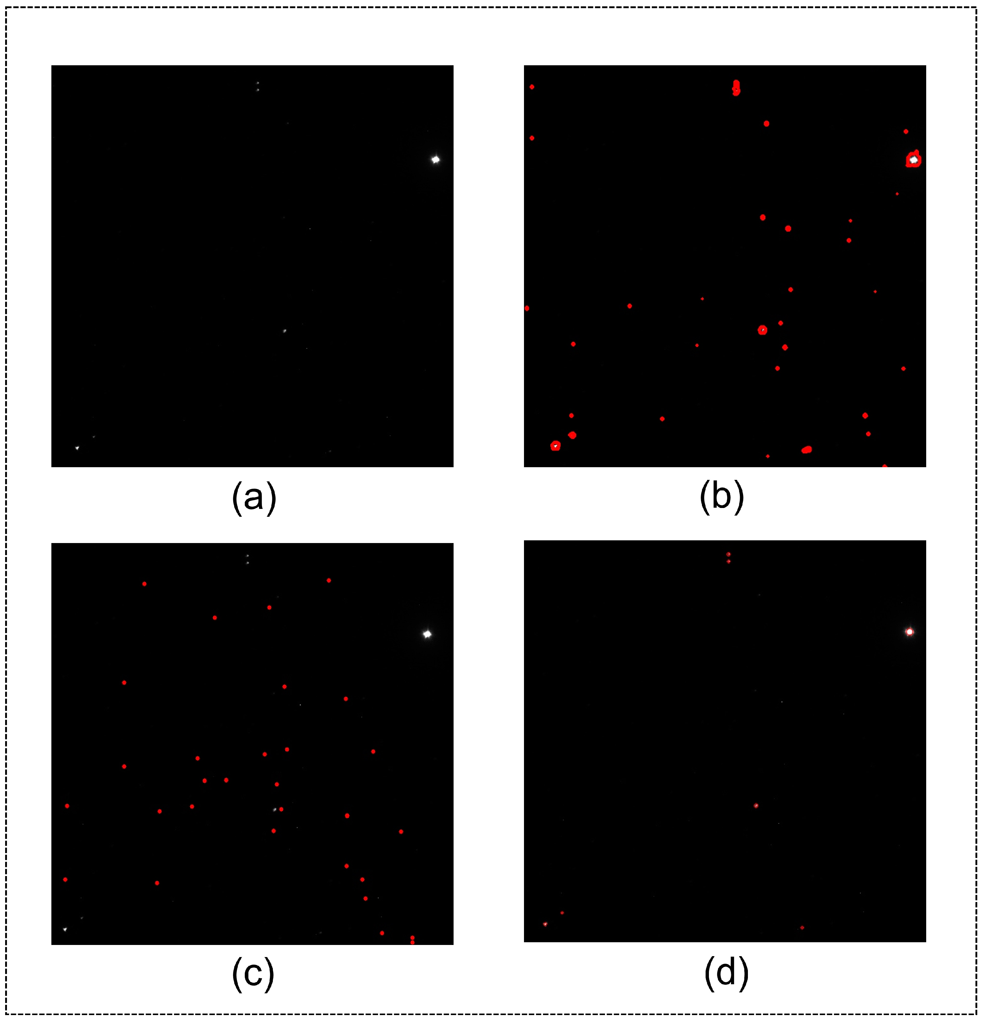
Figure 3a illustrates a section of the complete night sky image captured above the Yanqing station. The images were processed using the three algorithms mentioned above, with identified stars indicated in red. Figure 3b displays the experimental results obtained from implementing the morphological recognition algorithm, which incorrectly labeled certain interfering points as stars, resulting in the inaccurate identification of the results; however, it also correctly identified stars with larger areas. Figure 3c shows the results after employing the template-matching algorithm. The algorithm’s reliance on a specific template choice led to the misclassification of noise points as stars, compromising the accuracy of the recognition. 
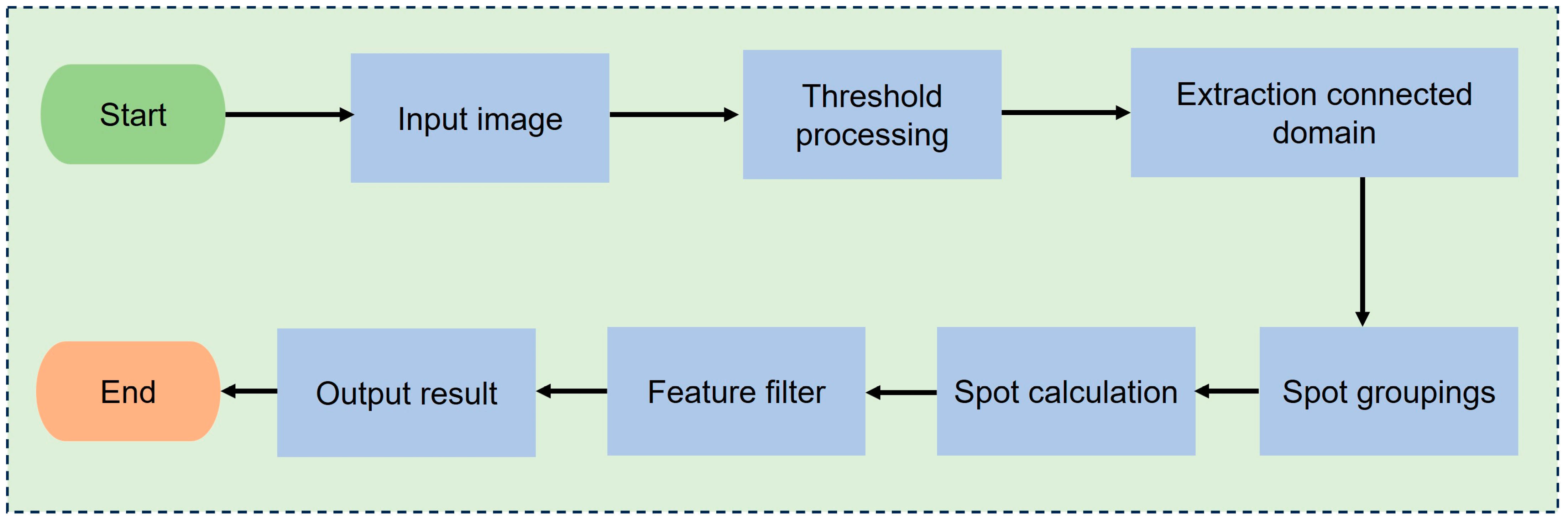
Figure 3d displays the results achieved with the spot detection algorithm. Unlike the two preceding recognition algorithms, the spot detection algorithm detected variations in brightness within the image to identify point targets and recognize the stars in the night sky image (Figure 4).
This process encompassed various steps, including threshold processing, connected domain extraction, spot grouping, spot calculation, and feature filtering. In the thresholding step, a starting threshold, a step threshold, and a termination threshold were established. To ensure the effective detection of stars of varying sizes and brightness, the starting threshold was set to 0. Stars were then detected from the lowest possible threshold to avoid missing any relatively small or weak stars. The algorithm’s sensitivity to the full range of star detection can be retained by setting these thresholds. To enhance algorithm efficiency, the step threshold was set to 3, circumventing unnecessary calculations and detections. A lower threshold value produces more candidate spots (or “speckles”), while a higher threshold value produces fewer candidate spots. Increasing the step threshold reduces computation while maintaining the ability to detect brighter spots. The termination threshold was set to 255 to ensure that the detected speckle covered the entire brightness range of the image. This setting allowed the algorithm to adapt to brightness and contrast changes in different images, improving its adaptability and robustness. Following this, connectivity components were extracted with different operators, and their centers were computed. Spot grouping involves setting a minimum distance between spots. Through trial and error, it was determined that reducing the minimum distance between spots may lead to over-segmentation, causing larger spots to be split into multiple smaller ones. Conversely, increasing the minimum spot distance may result in small spots being ignored or incorrectly filtered out. To improve the reliability and accuracy of speckle detection, we set the minimum speckle distance to 4. Any speckles in images closer than this threshold would be considered as a single speckle. The estimated center and radius of the speckle provide information regarding its location and size. The speckle’s location in the image can be determined and tracked by identifying its center, which allows for further analysis of its characteristics, trajectory, or other relevant information. The size of the speckle provides information about its scale characteristics and morphological features, which is important for identifying speckles of different sizes, analyzing changes in their shape, and eliminating the effect of noise. Finally, the spots were filtered based on color, area, roundness, inertia ratio, and convexity features. This robust approach effectively mitigated interference from dark spots and thermal noise in the night sky image through operations like spot grouping, spot calculation, and feature filtering. Evidently, this algorithm adeptly and accurately identified the stars in the night sky image. Furthermore, it exhibited control, robustness, tunability, and scalability, which makes it an advantageous approach.
Our subsequent analysis relied on the precise identification of stars in night sky images. 
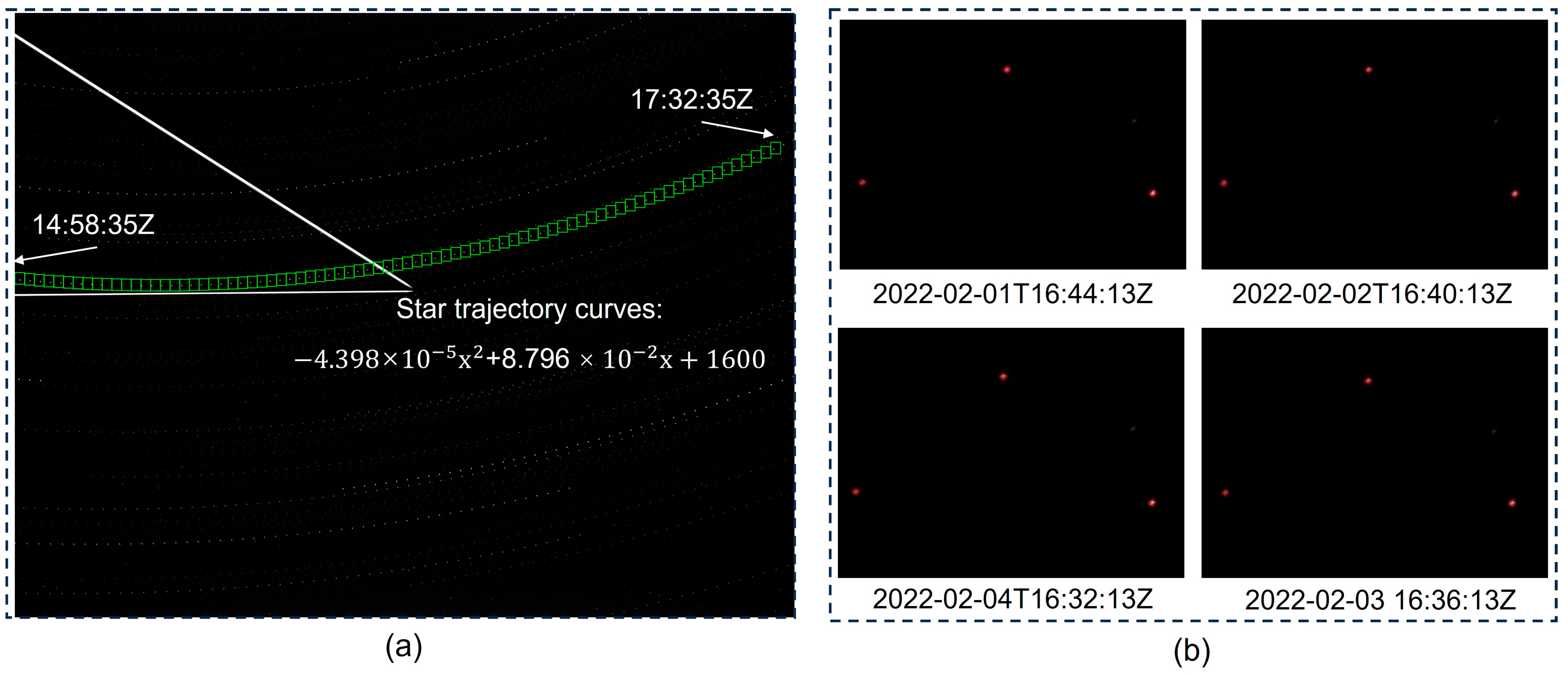
Figure 5a shows a composite of the gray values of the night sky images captured between 22:58 local time on 25 February 2022 and 01:32:35 on 26 February 2022 at the Yanqing station. A coordinate system was established with the image’s upper-left corner as the origin, and a trajectory of the star was fitted to allow for the constant monitoring of the star’s position within the camera’s field of view at any given moment. Because the camera’s field of view remains constant, and the Earth’s angular velocity is nearly uniform, with exceptions at the poles, a star that enters from the center of a wide-angle camera’s field of view has an approximate horizontal velocity of 35 pixels per minute and a vertical velocity of approximately 4 pixels per minute. It takes a minimum of 2 h for the star to exit the camera’s field of view. Further findings are presented in Figure 5b, where the night sky images corresponding to specific moments on four consecutive clear nights from 1 to 3 February 2022 were selected for demonstration. Without taking weather conditions into account, the appearance of a specific star above a LIDAR station through a fixed, wide-angle camera differed in time by approximately 3 min and 56 s when it reappeared at the same position in the camera’s field of view the following day. There are two primary causes of this phenomenon. First, the rotation of the Earth has a period of 23 h, 56 min, and 4 s, causing a slight shift in position relative to the stars at a given point in time. Second, the Earth rotates at a nearly constant speed of about 15 degrees per hour at all points except for the north and south poles. By leveraging these, it is possible to determine the position of the stars above the LIDAR station at any point during the night, thus providing a theoretical foundation for analyzing the area, brightness, and other characteristics of said stars on different dates.
We selected several night sky images for analysis based on corresponding moments on different nights. We identified the star positions within the images and established a consistent grayscale threshold. “Star area” refers here to the count of pixels exceeding the grayscale threshold, while “star brightness” pertains to the sum of the pixels with gray values exceeding the grayscale threshold. Over multiple nights, a substantial volume of data encompassing star count, area, and brightness above the LIDAR station was amassed. This dataset served as a comprehensive resource for the MUA-LIDAR system to predict the MRA.

2.3. Different MRA Prediction Models

In this study, we utilized the night sky images and echo signals collected by the Yanqing MUA-LIDAR station from January 2022 to April 2023 as data sources. Prior to analysis and modeling, the data were subjected to meticulous preprocessing procedures. The objective of these preprocessing steps was to eliminate superfluous information, including duplicates, missing data, and outliers, with the ultimate goal of bolstering the accuracy and quality of the data. Night sky image data were collected every 2 min, while echo-signal data were collected every 30 s. After downsampling the echo-signal data, they were combined and integrated with the data related to the number of stars, their respective areas, and brightness, which were derived from the processing of night sky images. These preprocessing steps served to refine the data, enhancing their accuracy, standardization, and completeness. This, in turn, optimized the performance of the machine learning algorithms and equipped them to effectively address practical challenges.
Linear multiple regression, nonlinear multiple regression, and summated autoregressive sliding average models were utilized to predict the MRA of the MUA-LIDAR system. Our aim was to compare the predictive ability of different models on this dataset. The model was implemented in Python, which provides powerful data processing and scientific computing libraries, giving it a significant edge in data processing and modeling analysis for various data-related and prediction issues in alignment with the objectives of this study.
Multiple regression modeling is a well-established statistical method for predicting the values of dependent variables by modeling the relationships between multiple independent (explanatory) variables and a single dependent (response) variable [28]. To predict the MRA, we performed a multiple regression analysis using the number, area, and brightness of stars as independent variables and the corresponding MRA data as dependent variables. We tested the data for feasibility to identify intrinsic patterns, from which a reasonable estimation of the MUA-LIDAR system’s MRA could be made. Based on the theory of multiple regression, linear and nonlinear model expressions were established as follows:
γ = β 0 + i = 1 3 β i x i
γ = f ( x 1 , x 2 , x 3 ) + β
where γ represents the MRA for the MUA-LIDAR system, x 1 is the number of stars, x 2 denotes the star’s areas, and x 3 signifies their brightness; these serve as the independent variables for the model inputs. β 0 β 3 represent the regression coefficients in the linear multiple regression model, while β indicates the regression coefficient in the nonlinear multiple regression model. These coefficients and independent variables are employed to predict the value of γ .
When using a linear multiple regression model to make predictions, the model parameters obtained were β 1 = 0.0173 , β 2 = 0.0062 , β 3 = 1.4619 , and β 0 = 51.7095 . When using a nonlinear multiple regression model to predict γ , it became apparent that the model intercept parameter was excessively large, while the regression coefficient parameter was of minute magnitude, measuring at 10 8 . To this effect, the nonlinear multiple regression model did not properly fit the training data and failed to capture the relationship between the independent and dependent variables. Furthermore, the intercept of the model was large, suggesting that the model could predict larger values of the dependent variable even in the absence of an independent variable. Hence, the nonlinear multiple regression model lacks robustness and is unfit for predicting the MRA. Therefore, we employed time series data (time, the number of stars, star area, and star brightness) as inputs for modeling and prediction using the ARIMA model.
ARIMA is a widely employed approach to modeling and predicting time series data [29]. It comprises three components: autoregression, integration, and moving average. ARIMA enables the modeling and prediction of key features, including trends, seasonality, and cyclical patterns. In an A R I M A ( p , d , q ) model, p represents the autoregressive order, d represents the number of differences, and q represents the moving average order. The modeling process typically encompasses three steps: model identification, parameter estimation, and model testing. Model identification entails determining the values of the autoregressive order p and the moving average order q by calculating the autocorrelation function and partial autocorrelation function of the time series. The number of differences d can be determined with a unit root test. By optimizing the A R I M A ( 1 , 1 , 1 ) model, we predicted MRA values by modeling time series data, including time, the number of stars, star area, and star brightness.
We utilized the mean squared error (MSE), root mean squared error (RMSE), and mean absolute error (MAE) metrics to evaluate the predictive performance of the model:
M S E = 1 n i = 1 n ( y ^ i y i ) 2
R M S E = 1 n i = 1 n ( y ^ i y i ) 2
M A E = 1 n i = 1 n | y ^ i y i |
where i represents the sequence number of prediction points, whereas y ^ i and y i indicate the predicted and actual values of the MRA at the i th prediction point, respectively; n represents the predicted data items. M S E is the average of the squared differences between the predicted values and actual values, which reflects both the predictive precision of the model and the magnitude of the prediction error. R M S E is the square root of M S E , which eliminates the effect of the square term in the MSE while retaining the magnitude of the error, making it easier to interpret. M A E is the average of the absolute differences between the predicted and actual values, which provides a measure of the model’s predictive accuracy and error magnitude; it more effectively eliminates outliers than M S E or R M S E . The predictive effectiveness of MRA values was comprehensively evaluated according to these three key metrics. Low MSE, RMSE, and MAE values indicate that the model has a high degree of predictive accuracy; high values suggest the opposite.
The linear multiple regression (MLRM) and ARIMA models were utilized to predict the MRA, and then their predictive performance was compared. As shown in Table 2, the ARIMA model outperformed the MLRM model, excelling in capturing temporal trends and periodic patterns in the time series data, including time, the number of stars, star area, and brightness.
Moreover, the ARIMA model has faster training and more precise and stable predictions, making it particularly suitable for practical applications. Conversely, linear regression models with multiple variables necessitate a high degree of linearity in the input data. Therefore, we selected the ARIMA model for predicting the MRA of the MUA-LIDAR system.

3. Results

We applied the ARIMA model to the data collected from the LIDAR stations in Yanqing, Lanzhou, and Urumqi. Night sky image features, including the number of stars, MRA, and other data from the Yanqing station for the entire nights of 8 January 2023 and 16 January 2023, were selected for this analysis.
Figure 6a displays the variations in the number of stars above the Yanqing LIDAR station during the night of January 8, amidst partly cloudy weather conditions. During the specific time intervals of 17:00–18:00 UTC and 20:00–21:00 UTC, observation conditions were unfavorable due to the low star count and MRA resulting from cloud cover. Figure 6b presents the actual and predicted MRA graphs for the entire night of January 8, while Figure 6c displays the absolute error curves of the true and predicted MRA values for that night. The analysis revealed an average error of 1.451 km in the all-night prediction, with a maximum error of 4.775 km. Figure 6d displays the fluctuations in the star count over the LIDAR station at Yanqing during the clear night of January 16. The observations revealed that the star count remained above 20 throughout the night. The number of stars fluctuated due to the rotation of the Earth, with stars continuously entering and exiting the camera’s field of view; this is properly reflected in the LIDAR observations. Figure 6e shows the actual and predicted MRA graphs for the night of January 16, while Figure 6f shows the absolute error curves of the true and predicted MRA values for the night of January 16. The analysis revealed an average error of 1.995 km in the all-night prediction, with a maximum error of 4.986 km. These results demonstrate that the ARIMA model is highly effective in predicting the MRA of MUA-LIDAR systems, regardless of the weather conditions over the LIDAR station throughout the night. Therefore, the model has robustness and high prediction accuracy.
Typically, sustained clear nighttime conditions (lasting more than 2 h) are optimal for obtaining high-quality echo-signal data, particularly for studies regarding the MUA. When the MRA of an MUA-LIDAR system falls below 35 km, the echo-signal data obtained is not suitable for conducting correlation studies involving the MUA. At this point, the MUA-LIDAR should be turned off. It is vital to note that making the decision about turning off requires a combination of factors, including meteorological conditions over the station. For instance, if there is a gale of force 5 or above at the station, solid particles such as sand and gravel may be brought by the gale, which can cause damage to precision equipment such as large-aperture telescopes, even if the MRA is still above 35 km at that time. Therefore, it is not appropriate to conduct observations under such conditions, and the MUA-LIDAR system should be turned off. This decision ensures the safety and normal operation of the equipment while protecting it from the risk of damage. Due to weather conditions and manual limitations, MUA-LIDAR systems often produce data of limited research significance upon observation initialization. As an example, consider the full-night observation conducted at the Yanqing station on 8 January 2023. The duration of the observation was approximately 516 min, of which the duration of valid data extended to about 382 min, resulting in a valid data rate of 74.03%.
However, after extracting the image features from the night sky data at the station and applying the ARIMA model for forecasting, we found that the effective observation time for the entire night increased to approximately 380 min, with 376 min of data obtained, resulting in an effective data rate of 98.95%. As depicted in Figure 7, there were 18 days of LIDAR observations during that January, totaling approximately 9507 min of observation time and an effective data rate of 79.39%. After applying the ARIMA model to analyze the night sky images and predict the MRA, the observation days extended to 24, the observation duration increased to 12,612 min, the effective data rate was 99.93%, and the observation duration was expanded by 32.67%.
In summary, real-time MRA prediction during MUA-LIDAR observation can reduce the need for excessive manual intervention and significantly increase the quantity of effective MUA-LIDAR observation days. Additionally, it offers an effective solution to managing intermittent severe weather conditions such as clouds and haze. This, in turn, can enhance the efficiency and data quality of MUA-LIDAR observations, reduce the resource consumption of LIDAR systems, and provide valuable support for the development of space weather intelligence.

4. Discussion

In response to the challenges posed by the tedious and labor-intensive manual operation of existing MUA-LIDAR systems, we investigated an intelligent operation system for the MUA-LIDAR system we developed in 2022. This system facilitates basic equipment operations with intelligent functions such as one-key on/off, status monitoring, emergency treatment, and remote monitoring. To further address the challenges related to weather conditions and human interference affecting MUA-LIDAR observations, an automatic weather identification system was established in 2023 [30]. This system assesses real-time weather conditions to determine their compatibility with LIDAR observation requirements and can provide early warnings for impending adverse weather conditions within the next two hours. This system ensures the safe operation of MUA-LIDAR systems and provides technical guarantees for effective observations. Based on these works, in this study, the automatic weather identification system is improved by using the MRA as the criteria for MUA-LIDAR to turn on observation. When the MRA of the MUA-LIDAR system is lower than 35 km, the MUA-LIDAR should be turned off, and when the MRA is greater than 35 km, the normal observation of MUA-LIADAR is maintained with attention to the other parameters of the external weather.
The predicting data of MRA are primarily derived from the MUA-LIDAR detection data and night sky images when the MUA-LIDAR is operating well. Therefore, when the prediction of MRA is accurate enough, it can also be used to evaluate the working status of MUA-LIDAR systems. If the predicted MRA value aligns with the value calculated through actual echo signals, it indicates that the MUA-LIDAR system is working well. Conversely, if the MRA derived from actual measurement data is significantly lower than the MRA predicted by the night sky images, it may suggest a problem with the operation of the MUA-LIDAR system. In such cases, we can adjust the operational status of the MUA-LIDAR system based on our previous work, including adjusting the laser energy, transmitter–receiver status, etc. [31,32]. Obviously, the MRA predictions are compared with the actual measurements, and necessary adjustments are taken to ensure that the MUA-LIDAR system is in good operating condition for a long time. This proactive maintenance strategy will help to obtain high-quality data in the long term and provide reliable support for subsequent scientific research.
Currently, automatic weather identification systems have been installed at five MUA-LIDAR stations located in Yanqing, Lanzhou, Urumqi, Mohe, and Zhangye. The system will undergo further refinement and enhancement based on local specifics as it is implemented at more MUA-LIDAR stations, resulting in improved prediction accuracy. Our research shows continual enhancements in the accuracy of MRA predictions. In future developments, the plan is to integrate the MRA prediction module into a holistic control system. The MRA will serve a twofold role: Not only does it serve as a criterion for activating the MUA LIDAR observation but it also serves as a measure of the operational status of the system. This evolution will make LIDAR control systems more intelligent, enabling the acquisition of substantial valid detection data with minimal human intervention. The research objectives will be achieved while maintaining the duration of LIDAR observations, thereby improving the overall quality of the data. After achieving these objectives, our control system will significantly reduce the need for manual oversight, thereby reducing the workload and stress on our personnel. The anticipation is to realize a truly unmanned operation, at which point the contributions of our work will have a lasting impact on the advancement of intelligent MUA-LIDAR systems.

5. Conclusions

In this study, we effectively utilized a comprehensive dataset of night sky images and echo signals to integrate the MRA as a novel indicator for assessing weather conditions at MUA-LIDAR stations. Through sophisticated big data analytics, we established a previously unreported correlation between night sky imagery and the MRA. Our testing phase, which lasted for a month, confirmed the model’s ability to predict the MRA with commendable precision and enhance the operational safety net for MUA-LIDAR systems. This innovation paves the way for more effective, economical, and intelligent MUA-LIDAR station operations, highlighting our contribution to the evolution of atmospheric monitoring technologies.

Author Contributions

Conceptualization, Z.L., G.Y. and J.W.; methodology, Z.L. and X.C.; software, Y.F. and W.X.; validation, L.L., X.C. and L.D.; data curation, Z.L., G.Y. and J.W.; writing—original draft preparation, J.W. and W.Z.; writing—review and editing, Z.L., G.Y., X.C. and W.X.; visualization, J.W.; funding, Z.L. and G.Y. All authors have read and agreed to the published version of the manuscript.

Funding

This research was funded by the National Key Research and Development Program of China (Grant Number 2022YFC2807201) and the National Natural Science Foundation of China (Grant Numbers 41474130, 41627804, and 41604130).

Data Availability Statement

Data are contained within the article.

Acknowledgments

We acknowledge the use of data from the Chinese MeridianProject. We acknowledge the Chinese MeridianProject to provide the equipment. We acknowledge the Specialized Research Fund for State Key Laboratories. We also acknowledge Ke Wei for his valuable assistance and support throughout the preparation of this paper. The authors would like to thank the editors and all the reviewers for their very valuable and insightful comments during the revision of this work.

Conflicts of Interest

Authors Yi Fan and Weiqiang Zhan were employed by the company uhan TopStar Optronics Technology Co., Ltd. The remaining authors declare that the research was conducted in the absence of any commercial or financial relationships that could be construed as a potential conflict of interest.

References

  1. Jiao, J.; Chu, X.; Jin, H.; Wang, Z.; Xun, Y.; Du, L.; Zheng, H.; Wu, F.; Xu, J.; Yuan, W.; et al. First Lidar profiling of meteoric Ca+ ion transport from∼ 80 to 300 km in the midlatitude nighttime ionosphere. Geophys. Res. Lett. 2022, 49, e2022GL100537. [Google Scholar] [CrossRef]
  2. Xia, Y.; Cheng, X.; Wang, Z.; Liu, L.; Yang, Y.; Du, L.; Jiao, J.; Wang, J.; Zheng, H.; Li, Y.; et al. Design of a Data Acquisition, Correction and Retrieval of Na Doppler Lidar for Diurnal Measurement of Temperature and Wind in the Mesosphere and Lower Thermosphere Region. Remote Sens. 2023, 15, 5140. [Google Scholar] [CrossRef]
  3. Eswaraiah, S.; Chalapathi, G.V.; Kumar, K.N.; Ratnam, M.V.; Kim, Y.H.; Prasanth, P.V.; Lee, J.; Rao, S.V. A case study of convectively generated gravity waves coupling of the lower atmosphere and mesosphere-lower thermosphere (MLT) over the tropical region: An observational evidence. J. Atmos. Sol.-Terr. Phys. 2018, 169, 45–51. [Google Scholar] [CrossRef]
  4. Chen, L.X.; Yang, G.T.; Wang, J.H.; Cheng, X.W.; Yue, C. Measurements of Lower Mesosphere Inversion Layers with Rayleigh Lidar over Beijing. Chin. J. Space Sci. 2017, 37, 75–81. [Google Scholar] [CrossRef]
  5. Xiong, J.; Yi, F.; Klostermeyer, J.; Rüster, R. The VHF observation and study of nonlinear interaction near mesopause. Chin. J. Radio Sci. 2000, 15, 84–89. [Google Scholar]
  6. Yang, Y.; Cheng, X.; Yang, G.; Xue, X.; Li, F. Research progress of lidar for upper atmosphere. Chin. J. Quantum Electron. 2020, 37, 566–579. [Google Scholar]
  7. Yi, F.; Zhang, S.; Yu, C.; Zhang, Y.; He, Y.; Liu, F.; Huang, K.; Huang, C.; Tan, Y. Simultaneous and common-volume three-lidar observations of sporadic metal layers in the mesopause region. J. Atmos. Sol.-Terr. Phys. 2013, 102, 172–184. [Google Scholar] [CrossRef]
  8. Jing, R.H.; Dai, K.; Zhao, R.X.; Cao, Y.; Xue, F.; Liu, C.H.; Zhao, S.R.; Li, Y.; Wei, Q. Progress and Challenge of Seamless Fine Gridded Weather Forecasting Technology in China. Meteorol. Mon. 2019, 45, 445–457. [Google Scholar]
  9. Du, L.; Zheng, H.; Xiao, C.; Cheng, X.; Wu, F.; Jiao, J.; Xun, Y.; Chen, Z.; Wang, J.; Yang, G. The All-Solid-State Narrowband Lidar Developed by Optical Parametric Oscillator/Amplifier (OPO/OPA) Technology for Simultaneous Detection of the Ca and Ca+ Layers. Remote Sens. 2023, 15, 4566. [Google Scholar] [CrossRef]
  10. Li, Z.C.; Chen, D.H. The development and application of the operational ensemble prediction system at national meteorological center. J. Appl. Meteorol. Sci. 2002, 13, 1–15. [Google Scholar]
  11. Glahn, H.R.; Ruth, D.P. The new digital forecast database of the National Weather Service. Bull. Am. Meteorol. Soc. 2003, 84, 195–202. [Google Scholar] [CrossRef]
  12. Engel, C.; Ebert, E.E. Gridded operational consensus forecasts of 2-m temperature over Australia. Weather. Forecast. 2012, 27, 301–322. [Google Scholar] [CrossRef]
  13. Kann, A.; Wang, Y.; Atencia, A.; Awan, N.; Dabernig, M.; Kemetmüller, J.; Meier, F.; Schicker, I.; Tüchler, L.; Wastl, C.; et al. Seamless probabilistic analysis and forecasting: From minutes to days ahead. In Proceedings of the EGU General Assembly Conference Abstracts, Vienna, Austria, 8–13 April 2018; p. 7962. [Google Scholar]
  14. Wang, W.; Cheng, X.; Liu, L.; Xia, Y.; Wang, J.; Huang, Z.; Shi, J.; Li, F. Lidar Technology and Preliminary Observation Results of Wind Temperature in the Middle and Upper Atmosphere at Lanzhou Yuzhong Station. Navig. Control 2022, 21, 250. [Google Scholar]
  15. Argall, P. Upper altitude limit for Rayleigh lidar. Ann. Geophys. 2007, 25, 19–25. [Google Scholar] [CrossRef]
  16. Xu, Y.; Lin, Z.; Yang, G.; Wang, J.; Cheng, X.; Li, F.; Yang, Y.; Du, L.; Jiao, J.; Xun, Y.; et al. Study on average characteristics of upper boundary of sodium layer in Yanqing, Beijing. Chin. J. Geophys. 2022, 65, 3714–3727. [Google Scholar]
  17. Tao, X.; Hu, Y.; Lei, W.; Cai, X. Application of empirical mode decom position in atmospheric echo processing of lidar. Laser Technol. 2008, 32, 590–592. [Google Scholar]
  18. Heese, B.; Flentje, H.; Althausen, D.; Ansmann, A.; Frey, S. Ceilometer lidar comparison: Backscatter coefficient retrieval and signal-to-noise ratio determination. Atmos. Meas. Tech. 2010, 3, 1763–1770. [Google Scholar] [CrossRef]
  19. States, R.J.; Gardner, C.S. Thermal Structure of the Mesopause Region (80–105 km) at 40°N Latitude. Part I: Seasonal Variations. J. Atmos. Sci. 2000, 57, 66–77. [Google Scholar] [CrossRef]
  20. Press, W.H.; Teukolsky, S.A. Savitzky-Golay smoothing filters. Comput. Phys. 1990, 4, 669–672. [Google Scholar] [CrossRef]
  21. Alvarez-Ramirez, J.; Rodriguez, E.; Echeverría, J.C. Detrending fluctuation analysis based on moving average filtering. Phys. A Stat. Mech. Its Appl. 2005, 354, 199–219. [Google Scholar] [CrossRef]
  22. Cui, X.; Zhou, X.; Fu, J.; Dai, J.; Liu, J. Research on level standards of high-impact weather over high-speed railway safety operation. J. Catastrophology 2016, 31, 26–30. [Google Scholar]
  23. Wan, B.; Kang, X.; Zhang, J.; Tong, Y.; Tang, G.; Li, X. Research on classification of dust and sand storm basic on particular concentration. Environ. Monit. China 2004, 20, 8–11. [Google Scholar]
  24. Chen, J.; Qian, W.; Han, J.; Lian, Z. An Approach for Radar Quantitative Precipitation Estimate Based on Z-I Relations Varying with Time and Space. Meteorol. Mon. 2015, 41, 296–303. [Google Scholar]
  25. Nozawa, S.; Kawahara, T.; Saito, N.; Hall, C.; Tsuda, T.; Kawabata, T.; Wada, S.; Brekke, A.; Takahashi, T.; Fujiwara, H.; et al. Variations of the neutral temperature and sodium density between 80 and 107 km above Tromsø during the winter of 2010–2011 by a new solid-state sodium lidar. J. Geophys. Res. 2014, 119, 441–451. [Google Scholar] [CrossRef]
  26. Sox, L. Rayleigh-Scatter Lidar Measurements of the Mesosphere and Thermosphere and Their Connections to Sudden Stratospheric Warmings; Utah State University: Logan, UT, USA, 2016. [Google Scholar]
  27. Deng, G.; Cahill, L. An adaptive Gaussian filter for noise reduction and edge detection. In Proceedings of the 1993 IEEE Conference Record Nuclear Science Symposium and Medical Imaging Conference, San Francisco, CA, USA, 30 October–6 November 1993; pp. 1615–1619. [Google Scholar]
  28. Wang, Z.; Miao, Z.; Yu, X.; He, F. Vis-NIR spectroscopy coupled with PLSR and multivariate regression models to predict soil salinity under different types of land use. Infrared Phys. Technol. 2023, 133, 104826. [Google Scholar] [CrossRef]
  29. Chodakowska, E.; Nazarko, J.; Nazarko, Ł.; Rabayah, H.S.; Abendeh, R.M.; Alawneh, R. ARIMA Models in Solar Radiation Forecasting in Different Geographic Locations. Energies 2023, 16, 5029. [Google Scholar] [CrossRef]
  30. Wei, J.; Cheng, X.; Yang, G.; Zhan, W.; Lin, Z. Weather Identification System for Normal Running of Middle and Upper Atmosphere Lidar. Laser Optoelectron. Prog. 2023, 60, 404–410. [Google Scholar]
  31. Xiao, J.; Dong, C.; Gao, F.; Zhan, W.; Cheng, X.; Yang, G. Development of Intelligent Operation System for Middle and Upper Atmosphere Lidar. Comput. Digit. Eng. 2022, 50, 2386–2392. [Google Scholar]
  32. Lin, Z.; Huang, K.; Xiong, W.; Wu, J.; Cheng, X.; Yang, G. Self-adaptive match algorithm for transmitter–receiver in the middle and upper atmospheric lidar. Opt. Commun. 2021, 488, 126811. [Google Scholar] [CrossRef]
Figure 1. Effects of MRA processing: (a) fair weather; (b) cloudy weather; (c) number of photons in echo signal versus detection altitude for single time point in (b).
Remotesensing 16 00536 g001
Figure 2. MUA-LIDAR power-on observation combined with a wide-angle camera to capture night sky images.
Remotesensing 16 00536 g002
Figure 3. Comparative effects of star recognition algorithm: (a) original image (partial); (b) morphological recognition processing; (c) template-matching processing; (d) spot detection processing.
Remotesensing 16 00536 g003
Figure 4. Flowchart of the spot detection algorithm.
Remotesensing 16 00536 g004
Figure 5. Star trajectory, star patterns in the same position on different dates with gray value superposition of night sky image: (a) star trajectory roadmap; (b) star position regularity map.
Remotesensing 16 00536 g005
Figure 6. Test results: (a) number of stars for the whole night of 8 January; (b) true and predicted values of detected MRA on 8 January; (c) absolute error of true and predicted values of detected MRA on 8 January; (d) number of stars for whole night of 16 January; (e) true and predicted values of detected MRA on 16 January; (f) absolute error of true and predicted values of detected MRA on 16 January.
Remotesensing 16 00536 g006
Figure 7. Comparison of the time of actual and systematic observations and the proportion of valid data.
Remotesensing 16 00536 g007
Table 1. Wide-angle camera parameters.
CameraValue
Exposure time2 s
Camera resolution5472 × 3648
Camera focus25 mm
Field of view27.34°
Gain1 dB
Table 2. Predictive effects of each algorithm.
AlgorithmMSERMSEMAE
MLRM19.6134.4293.428
ARIMA6.0862.4672.064
Disclaimer/Publisher’s Note: The statements, opinions and data contained in all publications are solely those of the individual author(s) and contributor(s) and not of MDPI and/or the editor(s). MDPI and/or the editor(s) disclaim responsibility for any injury to people or property resulting from any ideas, methods, instructions or products referred to in the content.

