Technical Note

Design of a Data Acquisition, Correction and Retrieval of Na Doppler Lidar for Diurnal Measurement of Temperature and Wind in the Mesosphere and Lower Thermosphere Region

1
School of Electronic Engineering, Nanjing Xiaozhuang University, Nanjing 211171, China
2
State Key Laboratory of Space Weather, National Space Science Center, Chinese Academy of Sciences, Beijing 100190, China
3
Innovation Academy for Precision Measurement Science and Technology, Chinese Academy of Sciences, Wuhan 430071, China
4
College of Science, Jiangsu University of Science and Technology, Zhenjiang 212100, China
*
Author to whom correspondence should be addressed.
Remote Sens. 2023, 15(21), 5140; https://doi.org/10.3390/rs15215140
Submission received: 28 July 2023 / Revised: 17 October 2023 / Accepted: 19 October 2023 / Published: 27 October 2023

Abstract

:
Based on the resonance fluorescence scattering mechanism, a narrowband sodium (Na) lidar can measure temperature and wind in the mesosphere and lower thermosphere (MLT) region. By using a narrowband spectral filter, background light noise during the day can be suppressed, allowing for continuous observations. To obtain full-diurnal-cycle temperature and wind measurement results, a complex and precise retrieval process is required, along with necessary corrections to minimize measurement errors. This paper introduces the design of a data acquisition unit for three frequencies in three directions of the Na lidar system in the Chinese Meridian Project (Phase II) and investigates the calibration and retrieval methods for obtaining diurnal temperature and horizontal wind in the MLT region, using a Na Doppler lidar with Faraday anomalous dispersion optical filter (FADOF). Furthermore, these methods are applied to observations conducted by a Na lidar in Beijing, China. The wind and temperature results over full diurnal cycles obtained from the all-solid-state Na Doppler lidar are reported for the first time and compared with temperature measurements from satellite, as well as wind observations from a meteor radar. The comparison demonstrates a reasonable agreement between the results, indicating the rationality of the lidar-retrieved results and the feasibility and effectiveness of the data correction and retrieval method.

Graphical Abstract

1. Introduction

It is widely recognized that, in the mesosphere and lower thermosphere (MLT) region, there exists a metal layer that includes metal atoms and ions such as sodium (Na), potassium (K), iron (Fe), nickel (Ni), calcium (Ca) and calcium ions (Ca+). The metal layer is situated in a critical region in the solar–terrestrial space environments and features complex dynamical and chemical processes. The research of the metal layer can help further our understanding of the atmospheric chemistry cycle and coupling of neutral and ionization components by analyzing the characteristics in morphological evolution and the seasonal and latitudinal changes of different atoms and ions in the metal layer. Moreover, the metal layer can serve as a tracer in the study of mid-upper atmosphere dynamics and thermodynamics and act as a clue to reveal the coupling process between the mid-upper atmosphere and the lower atmosphere [1,2].
Various methods can be used to detect metal layers, such as rockets, satellites and lidar, of which lidar is the most widely used. Metal layer detection lidars have been established in many parts of the world, and Na, Fe, K, Ca, Ca+ and Ni in the metal layer have been successfully detected using lidar [3,4,5,6,7,8,9,10,11]. In recent years, research on the detection of the metal layer has developed from a single lidar station to the integration of lidar networks and hybrid remote sensing systems. In China, the development of metal layer detection lidar has progressed rapidly in the past decade. With the support of the Chinese Meridian Project (Phase I), broadband Na lidars have been established in Beijing (40.42°N, 116.02°E), Wuhan (30.5°N, 114.4°E), Hefei (31.8°N, 117.3°E) and Haikou (19.5°N, 109.1°E) for measuring Na atom density [12]. Subsequently, multiple narrowband lidars were established in Hefei, Beijing and Lhasa (30°N, 90.5°E) for the simultaneous measurement of wind, temperature and density [13,14,15,16]. Lidars for detecting K, Ni, Ca and Ca+ have also been successfully installed at the Yanqing station in Beijing [17,18,19]. Currently, the Chinese Meridian Project (Phase II) is establishing lidars for the detection of various metal compositions (Na, K, Fe, Ni, Ca and Ca+) and wind and temperature of the Na layer in Mohe (53.5°N, 122.3°E), Lanzhou (36.0°N, 104.2°E) and Urumqi (43.3°N, 87.1°E) [20].
Na lidars are the most widely established system for detecting metal layer in the upper atmosphere due to the large scattering cross-section and higher abundance of Na atoms. This makes Na lidars an effective means of exploring the related atmospheric dynamics, thermodynamics and chemistry. Na lidars are based on a resonance fluorescence mechanism whereby Na atoms are excited by a 589 nm laser and emit photons when they return from an excited state to ground state. High-resolution detection of temperature and wind fields in the upper atmosphere is achieved using narrowband Na Doppler lidar through the use of a three-frequency ratio technique [5]. To obtain the required narrowband 589 nm pulsed laser, a pulsed dye amplifier (PDA) is seeded with a continuous-wave (CW) single-mode narrowband 589 nm laser. This can be outputted via a ring-cavity dye laser but is sensitive to temperature fluctuations and vibration, requiring human intervention. Alternatively, solid-state Na lidar systems using a sum-frequency generation (SFG) of 1064 nm and 1319 nm lasers or second harmonic generation (SHG) of 1178 nm laser techniques have been developed to reduce intervention [15,16,21]. The development of Na lidar technology has led to increased stability and reliability of the lidar system, enabling many more investigations in atmospheric dynamics and chemistry. The effective fluorescence scattering cross-sections of Na atoms change with background atmospheric temperature and wind, and temperature and line-of-sight (LOS) wind can be retrieved from Doppler-broadening and the shifting of the observed Na D2 spectrum through calculating intensity ratios of three-frequency echo signals [22]. The three-frequency 589 nm laser can be obtained with an acousto-optic modulation (AOM) unit to cyclically up- and down-shift the locked seed laser frequency from v a to v + = v a + δ v and v = v a δ v ; v a is the laser frequency corresponding to the Na D2a peak; and δ v is the frequency shift amount. A free-space design of AOM unit will increase the challenge of optical adjustment and maintenance. The use of a fiber-coupled AOM unit largely reduces manual intervention and promotes automated operation of Na lidar [15,16].
The diurnal measurement of the metal layer by lidar can provide an important data source for studying dynamics and photochemical processes in the MLT region. However, daytime observations face challenges due to a strong background noise, which submerges the signal of the metal layer. To achieve daytime observation, the use of narrowband spectral filters is essential to suppress background light. In order to effectively suppress the background noise and improve the signal-to-noise ratio (SNR), Faraday anomalous dispersion optical filter (FADOF) is utilized in the lidar receiver [23,24]. With FADOF, the lidar returns will depend on both the lidar efficiency and the transmission function of the utilized FADOF. The fluorescence echo spectrum frequency positions corresponding to three different operating frequencies of lasers are different, and after passing through the filter, the echo spectrum will be attenuated to varying degrees. Normalization of the resonance fluorescence signals with Rayleigh signals from a reference altitude is generally used, which can help eliminate the measurement uncertainty induced by the laser energy fluctuations and variations of atmospheric transmittance, which is difficult to measure. The Rayleigh signals will also be influenced by the FADOF, and the effective FADOF transmission of the Rayleigh scattering signal is different from that of the fluorescence signal. Therefore, it is necessary to simultaneously correct the attenuations of both the Rayleigh scattering and Na fluorescence echo spectrum at different frequencies during data analysis. Additionally, a high power aperture is often employed for the Na lidar to achieve a high SNR and decrease the measurement uncertainty induced by photon noise. However, this may lead to the nonlinearity of photon counting due to the pulse pile-up effect, which results in large retrieval bias. The possible saturation effect of PMT should also be corrected to improve the measurement reliability.
This paper presents the design of a data acquisition unit of the Na lidar system in the Chinese Meridian Project (Phase II) and investigates the calibration and iterative retrieval methods of wind and temperature from diurnal Na Doppler lidar returns with FADOF. The temperature and horizontal wind results from continuous observations in the MLT region over Yanqing, Beijing, are obtained and compared to those from satellite and a nearby meteor radar.

2. Methodology

Na density, temperature and radial velocity in the mesopause region can be determined by measuring the backscattered photon count from the Na layer at three different frequencies within the fluorescence absorption spectrum of Na atoms. In order to derive these parameters accurately, the probing frequencies need to be carefully selected to minimize the measurement errors. Numerical techniques for solving nonlinear systems of equations can be employed to accurately derive these atmospheric parameters. Meanwhile, the performance of three-frequency Doppler lidars can be improved by optimizing the determination of probing frequencies and the integration period, using nonlinear numerical techniques, as suggested by Gardner and Vargas [25]. In this paper, we employ the three-frequency ratio technique to derive the temperature and radial velocity [5]. The theoretically calculated temperature ratio (RT) and wind ratio (RV) can be expressed by the effective scattering cross-sections at three frequencies as follows [9]:
R T ( z ) = σ e f f v + , Z + σ e f f ( v , Z ) 2 σ e f f ( v a , Z )
R V ( z ) = σ e f f v + , Z σ e f f ( v , Z ) σ e f f ( v a , Z )
σ e f f v = 1 2 π σ e e 2 f 4 ε 0 m e c n = 1 6 A n e x p v n v ( 1 V R c ) 2 2 σ e 2
where v a , v + and v are the three laser frequencies of Na lidar for wind and temperature measurement; σ e f f is the effective scattering cross-section of Na atoms; f is the oscillation intensity of the D2 line; A n is the linear intensity of the six electric dipole moments for D2 line transitions; v n is the frequency relative to weight center of the six discrete spectral lines for D2 transitions; V R is the LOS velocity of Na atom relative to the direction of laser beam; σ e = σ D 2 + σ L 2 is the total spectral width; σ L is the RMS of laser spectral width; σ D = v 0 k B T m c 2 is the Doppler broadened spectral width; T is the atomic temperature; k B is Boltzmann constant; m is the mass of single Na atom; v 0 is the resonant frequency of atomic transition; and c is the speed of light. Based on Equations (1) and (2) and the functional relationship between effective scattering cross-section and temperature and LOS wind provided by Equation (3), the temperature and LOS wind can be retrieved from the measured temperature and wind ratios (RT and RV) calculated from the lidar echo photons.
There is meteor radar available near Yanqing station (approximately 40 km away), Beijing, that can provide horizontal wind data as a reference for the lidar-retrieved results. In this study, we utilized a set of observational data obtained at Yanqing station by an all-solid-state Na lidar as examples to illustrate the rationality and effectiveness of the presented data analysis method. The all-solid-state Na Doppler lidar was constructed at Yanqing station, Beijing, in 2016 for measuring nocturnal temperature and horizontal wind in the mesopause region [15] and was further upgraded to enable diurnal measurements by incorporating FADOF in late 2019. Recently, this lidar system was relocated to Mohe as a part of the Chinese Meridian Project (Phase II).
To maximize the measurement sensitivity of wind/temperature and reduce the measurement uncertainty caused by photon noise, δ v is typically set to 630 MHz [13,14,16,21,22,26]. The Na Doppler lidar system built at Yanqing, Beijing, uses an SFG of 1064 nm and 1319 nm to obtain a 589 nm laser, and a fiber-coupled AOM unit is used to generate three working frequencies by up- and down-shifting the laser frequency. The resonant cavity of the pulse laser changes when the laser frequency is rapidly switched among the three working frequencies. To ensure seed injection, the longitudinal mode spacing of 1064 nm Nd:YAG pulse laser cavity needs to be considered when selecting the frequency shift to optimize the pulse establishment time and achieve cavity mode matching. The longitudinal mode spacing is given as follows:
Δ v = c 2 n L
where nL is the total optical path length of the pulsed laser cavity. Considering the mechanical cavity length and optical path difference of the Nd:YAG crystal rod, pucker box and lens comprehensively, the total optical resonance cavity length of the 1064 nm pulse laser is about 2303.19 mm. According to Equation (4), the corresponding longitudinal mode spacing is calculated to be 65 MHz. The integral multiple of Δ v closest to 630 MHz is 585 MHz, which enables all three different working laser frequencies to be well matched to the cavity mode of the pulsed laser cavity. Therefore, for the Yanqing Na lidar system, the shift amount ( δ v ) is set to 585 MHz [15]. Figure 1 shows the theoretical 2D calibration curves that convert intensity ratios (RT and Rv) to temperature and LOS wind (T and V) with a frequency shift amount of 585 MHz. For more details on the lidar system, please refer to [15].

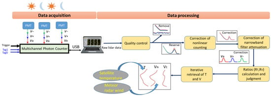
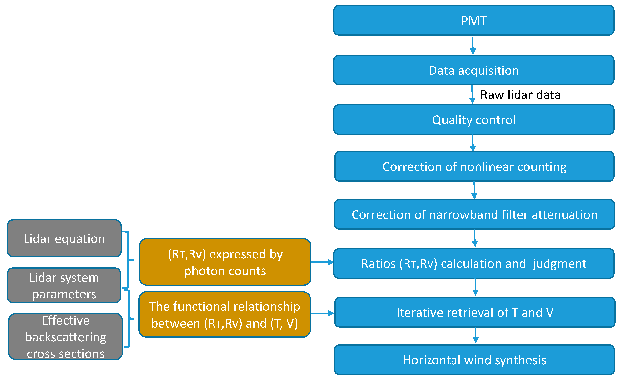
3. Data Acquisition and Processing

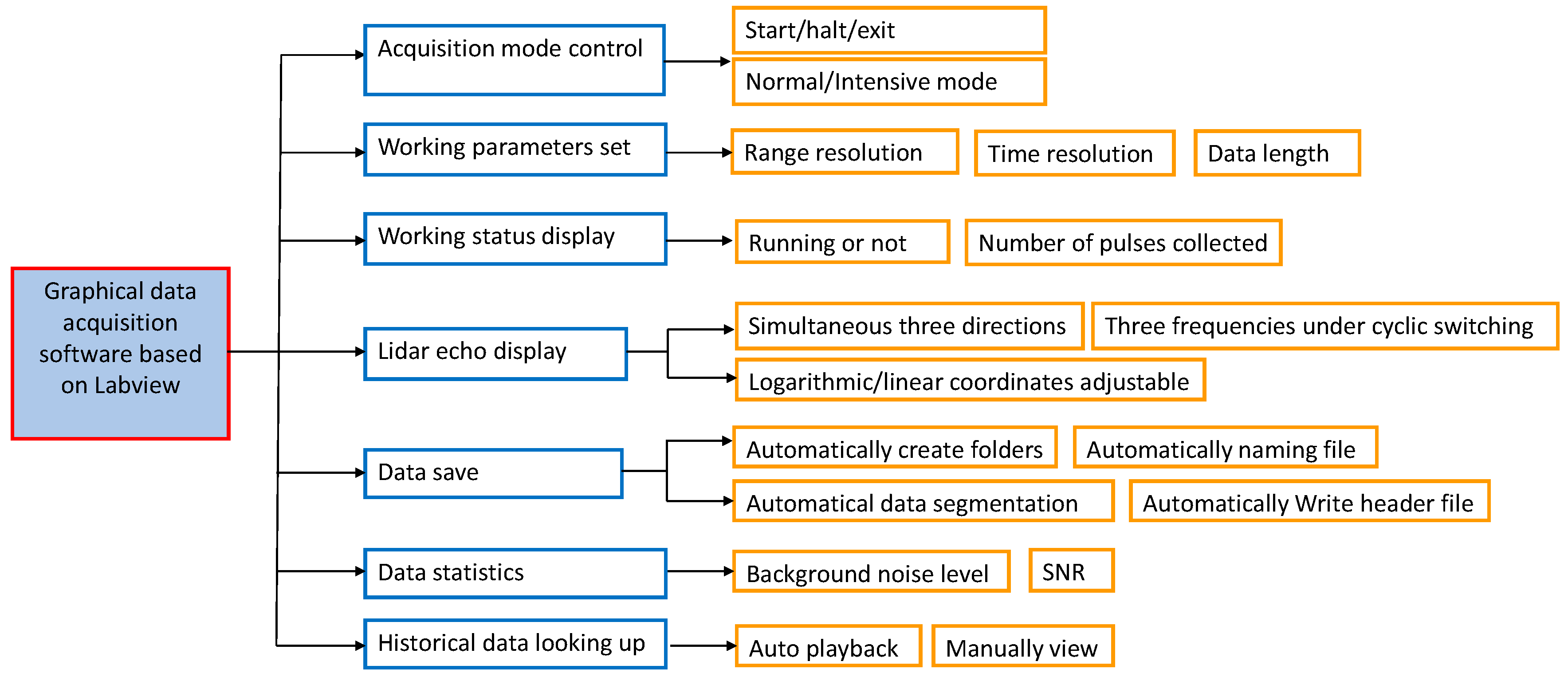
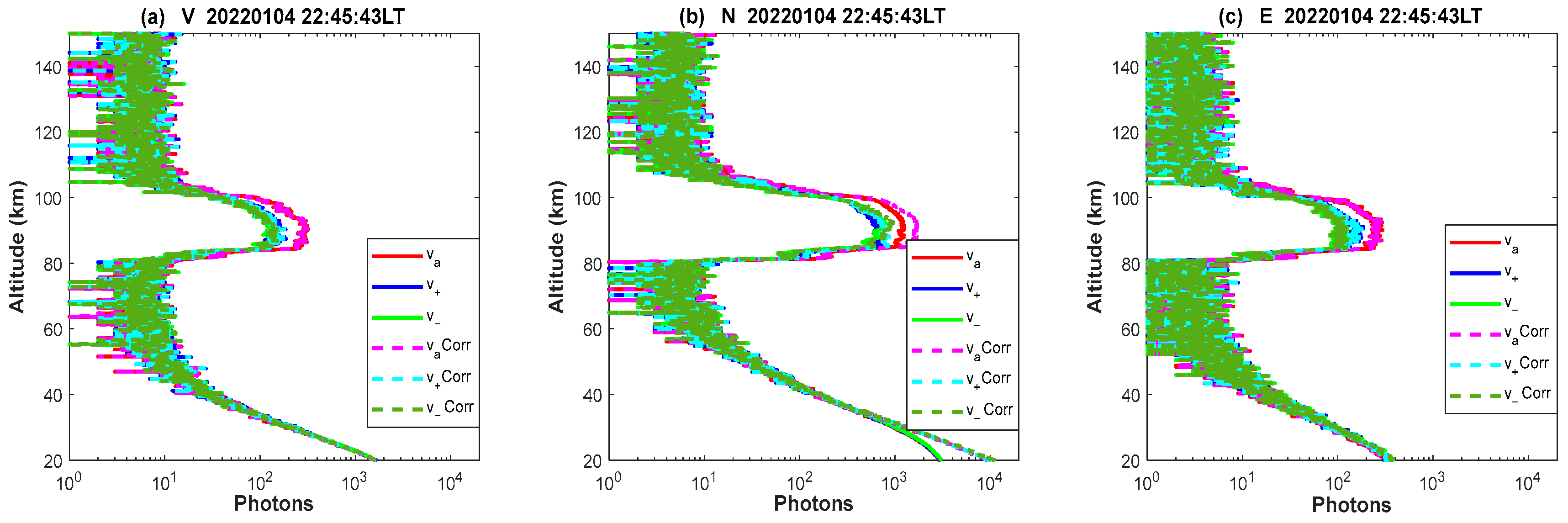
3.1. Data Acquisition of Three Frequencies in Three Directions

The pulsed 589 nm laser is split into three beams that are directed towards zenith, 30° off zenith to the west/east and 30° off zenith to north/south, respectively. The backscattered resonance fluorescence signals are received by three telescopes and passed through the FADOF to suppress background noise before being received by the photomultiplier tube (PMT). In order to record the pulsed electrical signal, the Model P7882 photon counting card from FastComtec is utilized. This card has two input channels and can be used to acquire the echo signal from three observational directions simultaneously. However, two cards are required for complete three-directional observation. Recently, an updated Model MCS8A has been used to acquire data for the Na Doppler lidar system in the Chinese Meridian Project (Phase II). This card can be configured with more channels, permitting lidar returns from three directions acquired by a single card. Additionally, the MCS8A has a USB interface for easy connection with a computer. The upgraded photon counting card allows for the recording of lidar photons with a minimum dwell time (time-bin width) of 800 ps. This means that the lidar echoes received within each time bin, relative to the start pulse, are summed. As a result, a range resolution of 0.12 m is achieved by multiplying the time-bin width by the speed of light divided by 2 (range resolution = time-bin width *c/2, where c represents the velocity of light). Typically, in the Chinese Meridian Project (Phase II), the range resolution for Na lidar observations is set to ~30.72 m (256 bins), with a temporal resolution of 60 s (normal mode, where echoes from 1800 laser pulses are summed, considering a laser pulse repetition rate of 30 Hz) or 10 s (intensive mode, where 300 pulses are summed).
The output laser frequency is cyclically switched among v a , v + = v a + δ v and v = v a δ v . The lidar echoes corresponding to these three different working frequencies are integrated in a cyclical manner. To organize the data storage channels of the three working frequencies, two TTL signals controlling the working sequence are used for classifying and tagging the data. The TTL signals are provided on the tag connector of the data acquisition card and serve as strobe signals. These signals indicate the “active” laser frequency and segment the data memory accordingly. Specifically, the tag bit patterns of 00, 01 and 10 correspond to v a , v + and v , respectively. When TTL 1 and 2 are low, the lidar echoes corresponding to the working frequency v a are accumulated in the first segment of the data memory. If TTL 1 is low and TTL 2 is high, the lidar echoes corresponding to working frequency v + are accumulated in the second segment, and so on. The enabled tag bits to shift the lidar spectrum in memory based on the actual tag input, allowing for the acquisition of three separate spectra, each corresponding to one of the three different working frequencies marked by tag bits. The LabVIEW-based program running on the host computer is used to display and store the data of each storage area. The data file also records operating parameters, such as lidar location, elevation, observational date, starting and ending time, data length and laser repetition frequency, to facilitate secondary data development. Additionally, the data acquisition program integrates a data statistics module that calculates the background noise, Rayleigh scattering signal and Na fluorescence signal in real time to monitor the quality of observational data. The design of the data acquisition program is shown in Figure 2.

3.2. Data Processing

Retrieving the wind and temperature from raw data entails several processing steps, including quality control, correction of PMT nonlinear counting, correction of narrowband filter attenuation, ratios calculation and check, iterative retrieval of temperature and LOS wind from ratios and horizontal wind synthesis, as illustrated in Figure 3.

3.2.1. Quality Control of Raw Lidar Data

The lidar data quality may be influenced by weather conditions and changes in the system’s working status, and it is essential to exclude abnormal or unqualified data files beforehand. This can be achieved through manual inspection or software-based automatic diagnosis. While manual inspection relies on subjective experience and may not be as efficient, it can be useful for cases where abnormal data and qualified data are difficult to discern and may cause erroneous judgment by software-based automatic diagnosis. On the other hand, software-based automatic diagnosis can efficiently detect data files that do not meet the set standards or criteria in the program and allow for batch processing. However, the data diagnosis standards require careful consideration. The quality of the raw data can be assessed by analyzing the signal-to-noise ratio (SNR). In this study, we employed the SNR of raw photon data to conduct a preliminary automatic batch screening of the lidar data. Specifically, we calculated the Na peak signal-to-noise ratio ( S N R N a ) and Rayleigh signal-to-noise ratio ( S N R R a y ) as follows:
S N R N a = S N a / N o i s e N a
S N R R a y = S R a y / N o i s e R a y
where S N a and S R a y represent the Na fluorescence peak signal and Rayleigh echo signal at the reference height (~32 km), respectively, after subtracting the background noise ( S N a = N N a N B a c k g r o u n d ; S R a y = N R a y N B a c k g r o u n d ). The values of N N a and N R a y can be directly obtained from the lidar photon profiles, and N B a c k g r o u n d is calculated as the average photon count in the altitude range of 180~200 km. The photon counting noise is described by the Poisson statistical distribution, and it is estimated as the square root of the photon counts ( N o i s e N a = N N a ; N o i s e R a y = N R a y ).
Poor-quality data in the lidar raw data can arise from various sources, including cloud-induced attenuation of echo signals, mismatches in the lidar’s field of view during system adjustment and noise interference. We aim to strike a balance between preserving valuable data and mitigating the impact of poor-quality measurements resulting from these factors. Given that the calculation of RT and RV, as well as the iterative retrieval of temperature and wind, relies on accumulated raw photon counting profiles in time and altitude, we typically set the threshold for the SNR of the raw data to 1 to retain as much of the available raw data as possible. Raw photon profiles with SNRNa ≥ 1 and SNRRay ≥ 1 are preserved for subsequent data processing. This threshold ensures that only raw data with a minimum level of quality, indicated by an acceptable SNR, is included in the subsequent analysis.

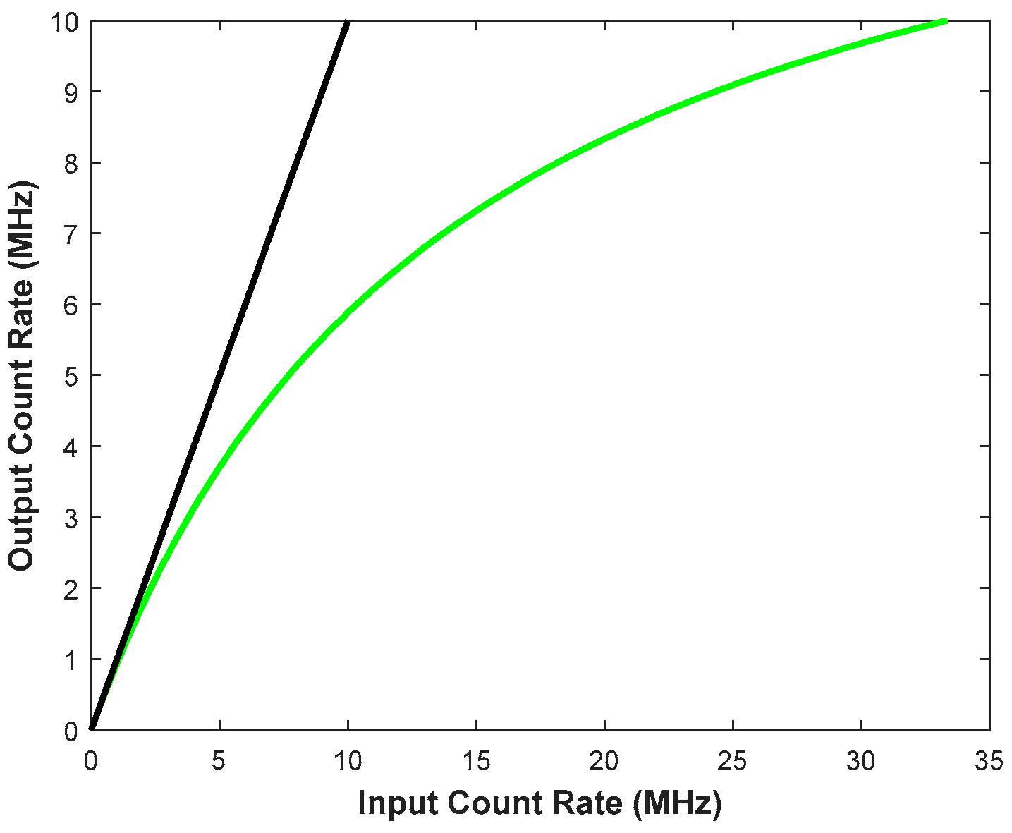
3.2.2. Correction of PMT Nonlinear Counting

To detect lidar echo photons, we use PMT (model H7421-40 from Hamamatsu), which has high quantum efficiency (40% at peak wavelength). However, strong echo signal may cause nonlinearity in the PMT counting, leading to detection signal distortion. A severe saturation effect can cause significant bias or discrepancy in the derived temperature and LOS wind. Hence, checking for saturation and correcting the effect, if present, are necessary during data processing. During data processing, we calculate the photon count rate for each lidar profile. If the maximum count rate above 30 km exceeds the threshold within the PMT linear count range (~1.5 MHz/s for H7421-40, as per the manufacturer’s specifications), it gets corrected according to the PMT correction curve. The green line in Figure 4 is a PMT correction curve given by Hamamatsu for PMT in H7421-40 series. A more accurate correction relationship can be obtained in a laboratory setting by comparing the PMT output count rates against the input count rates from a known light source [27]. For calculating the heat flux, which is a small quantity where even a minor bias can be significant, the PMT correction curve can be further revised based on observational data, particularly when the PMT count rate is very high [27].
Figure 5 shows an example of the raw photon counts profiles (solid lines) and the corresponding profiles with PMT nonlinearity correction (dashed lines). Each direction has an integration time of 100 s (1500 pulses at a 15 Hz repetition rate for the narrowband Na lidar at YanQing, Beijing). As can be seen, the north direction shows relatively larger raw photon counts compared to the other two directions, mainly due to the different beam splitting ratio. By calculating the photon counting rate for each frequency, it is observed that the echo signals from zenith and east are not affected by PMT saturation, and the profiles before and after correction are nearly identical. However, a certain amount of correction is added for the north direction due to the PMT counting nonlinearity. As the effective cross-section at v a is the largest, the echo photons at frequency v a are more likely subjected to the nonlinearity effect. It is seen that the correction amount for the photon profile at v a from the north direction is significant around the Na layer peak and below ~30 km. The more serious underestimation of photon counts at v a compared to v ± leads to an increase in RT (and thus the derived temperature), as can be seen from the pink solid line in Figure 6.
Figure 6a displays an example of the derived temperature profiles measured in three directions before and after PMT correction. The data are processed in 30 min temporal and ~1000 m range resolutions. The temperature results from east and zenith between 82 and 103 km show good consistency, and the results before and after correction are identical (the black and blue dashed and solid lines overlap). A high photon count rate in the north direction without correction produces a large positive temperature deviation up to 40 K in the altitude range of 85~98 km (pink solid line). After correction, the temperature profile in the north direction (the pink dashed line) aligns well with the results obtained from the zenith and east directions. This agreement indicates the feasibility and effectiveness of the data correction method. The Sounding of Atmosphere Broadband Emission Radiometer (SABER) onboard the Thermosphere Ionosphere and Mesosphere Electric Dynamics (TIMED) satellite provides temperature profiles covering the MLT region [28]. Dawkins et al. [29] demonstrated that SABER results were statistically similar to lidar temperature profiles. However, it is important to note that SABER retrieves the temperature from the 15 um CO2 emission, and the local thermodynamic equilibrium (LTE) approximation is not applicable above an altitude of ~75–80 km for the CO22) vibrational levels involved in the formation of the 15 um radiance. The presence of significant non-LTE effects introduces uncertainty in the calculation of the CO2 vibrational level populations [30,31]. Additionally, there are differences in the sampling size and spatiotemporal collocation between the available SABER and lidar results [29]. Therefore, quantitatively validating the individual lidar-retrieved temperature profiles using SABER results presents significant challenges. In this study, we utilized SABER as an indirect reference to provide auxiliary verification of the effectiveness of the data correction method in reducing potential systematic errors. Figure 6a, shows a SABER temperature profile (red crosses) that we plotted that was sampled during the lidar measurement time interval and was closest to the lidar location. The comparison showed that the lidar temperature profile with correction (pink dashed line) exhibits a similar changing range and trend to the SABER result. Figure 6b,c illustrate the zonal and meridional winds with a resolution of 1 h and ~2 km measured by lidar, respectively. The zonal wind profile (the blue dashed and solid lines overlap, indicating that the east direction was not saturated) essentially agrees with the meteor radar result (black solid line, temporal and height resolution: 1 h, 2 km, 40.3°N, 116.2°E), the wind deviation between them is relatively small, i.e., between 82 and 96 km. However, the originally derived meridional wind without correction (pink solid line) shows significant deviation around 92 km due to the PMT nonlinearity effect of lidar echo from the north direction around the Na layer peak. The PMT nonlinearity correction leads to a more accurate meridional wind profile (pink dashed line) that is closer to the result from radar (black solid line). The temperature and wind results in Figure 6 show that temperature is more sensitive to PMT nonlinearity than wind, a finding that is consistent with previous studies by Liu and Guo [27].

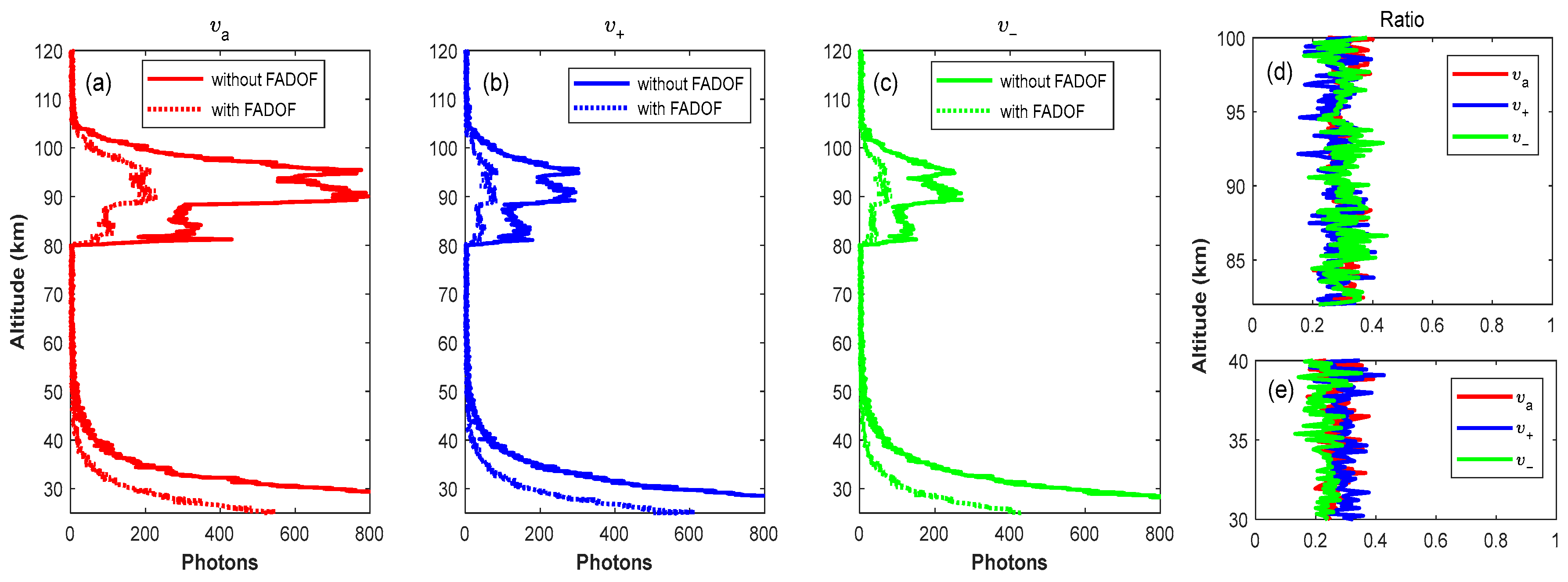
3.2.3. Correction of Narrowband Filter

Through normalization using the atmospheric Rayleigh echo signal at a reference altitude and by using the method of the three-frequency ratio, it is possible to retrieve wind and temperature while disregarding many unknown atmospheric and system parameters. After the elimination of abnormal data, the correction of PMT saturation, background subtraction, normalization using the Rayleigh signal around the reference height (~32 km) and the correction of the extinction of the Na layer, the resulting normalized photon counts at height Z can be expressed as follows:
N n o r m ( v , z ) = N N a v , Z N B N R v , Z R N B E 2 λ , Z
where N N a is the lidar received Na fluorescence signal at height Z and laser frequency v ; N R is the atmospheric Rayleigh scattering signal at a referenced height, Z R ; N B is the background noise; and E is the extinction coefficient due to the absorption of the atomic layers, and it depends on laser frequency and height [9]. In order to decrease uncertainty caused by Rayleigh signal perturbations at the reference height, counts can be summed over a number of range bins, for example, between 31 and 33 km as NR. To suppress background noise, the narrow passband of FADOF is effective, but it attenuates both the fluorescence signal from the Na layer and the Rayleigh signal. As a result, the photon counts must be corrected before calculating wind and temperature ratios. The transmission function of the FADOF in general should be measured by scanning the laser frequency and used to calibrate the attenuation of Rayleigh and fluorescence echo signals by FADOF.
For Na D2 transition, there are 10 excitation–emission pathways and eight emission frequencies. The relative transmission through FADOF for different emission frequencies is different, and both the Faraday filter function and the backward fluorescence emission rates, as well as the exact frequencies for 10 pathways, should be taken into account during the retrieval of wind and temperature [22,24]. For the Rayleigh scattering spectrum, which is centered at the laser frequency, the main difference in Faraday filter attenuation for three working frequencies mainly depends on the spectral center location relative to the Faraday filter function [22]. As the transmission function of the FADOF is stable, in this study, we calibrate the attenuation of Rayleigh scattering and Na fluorescence through FADOF by using the ratio of lidar echo signals before and after inserting the FADOF. Considering the different levels of attenuation by FADOF to Na fluorescence signal and Rayleigh scattering signals for the three working frequencies ( v a , v + , v ), the correction factor can be set as r v i = T v i R a y / T v i N a ; and T v i R a y and T v i N a ( v i = v a , v + , v , which are the three working frequencies) are, respectively, the effective Rayleigh and Na fluorescence signal transmittance through the Faraday filter. T v i R a y = N v i R a y 1 / N v i R a y 2 , T v i N a = N v i N a 1 / N v i N a 2 ,   N v i R a y 1 , N v i N a 1 , N v i R a y 2 , N v i N a 2 are, respectively, the Rayleigh echo signal at the reference height and Na fluorescence signal detected by the lidar with and without FADOF. For nocturnal observations without FADOF, r v i = 1 .
Figure 7a–c show the examples of the photon count profiles at the three operating frequencies before and after inserting the FADOF in the lidar receiver. In a short time, the variation in Na density and temperature can be ignored and the ratio of signals with and without FADOF can be considered mainly caused by the attenuation by the FADOF. The different attenuation by the FADOF for fluorescence and Rayleigh scattering of the three frequencies can be seen in Figure 7d,e. We average over a number of range bins centered at Na layer peak and reference height, for example, between 85 and 95 km for fluorescence and between 29 and 31 km for the Rayleigh signal, to obtain T v i R a y and T v i N a . It is worth mentioning that, for the simultaneous three-directional measurements, a single-channel FADOF is utilized for each direction in the receiver of the all-solid-state Na lidar, considering the compactness of the detection unit. In comparison to the dual-channel design presented in Xia et al. [32], the transmittance is reduced by half, approximately 0.3, as depicted in Figure 7d,e. After obtaining the correction factors of FADOF attenuation for three frequencies, the temperature and wind measurement ratios, i.e., R T and R V , can be given as follows:
R T ( z ) = N n o r m ( v + , z ) r v + + N n o r m ( v , Z ) r v 2 N n o r m ( v a , z ) r v a
  R V ( z ) = N n o r m v + , z r v + N n o r m ( v , Z ) r v N n o r m ( v a , z ) r v a

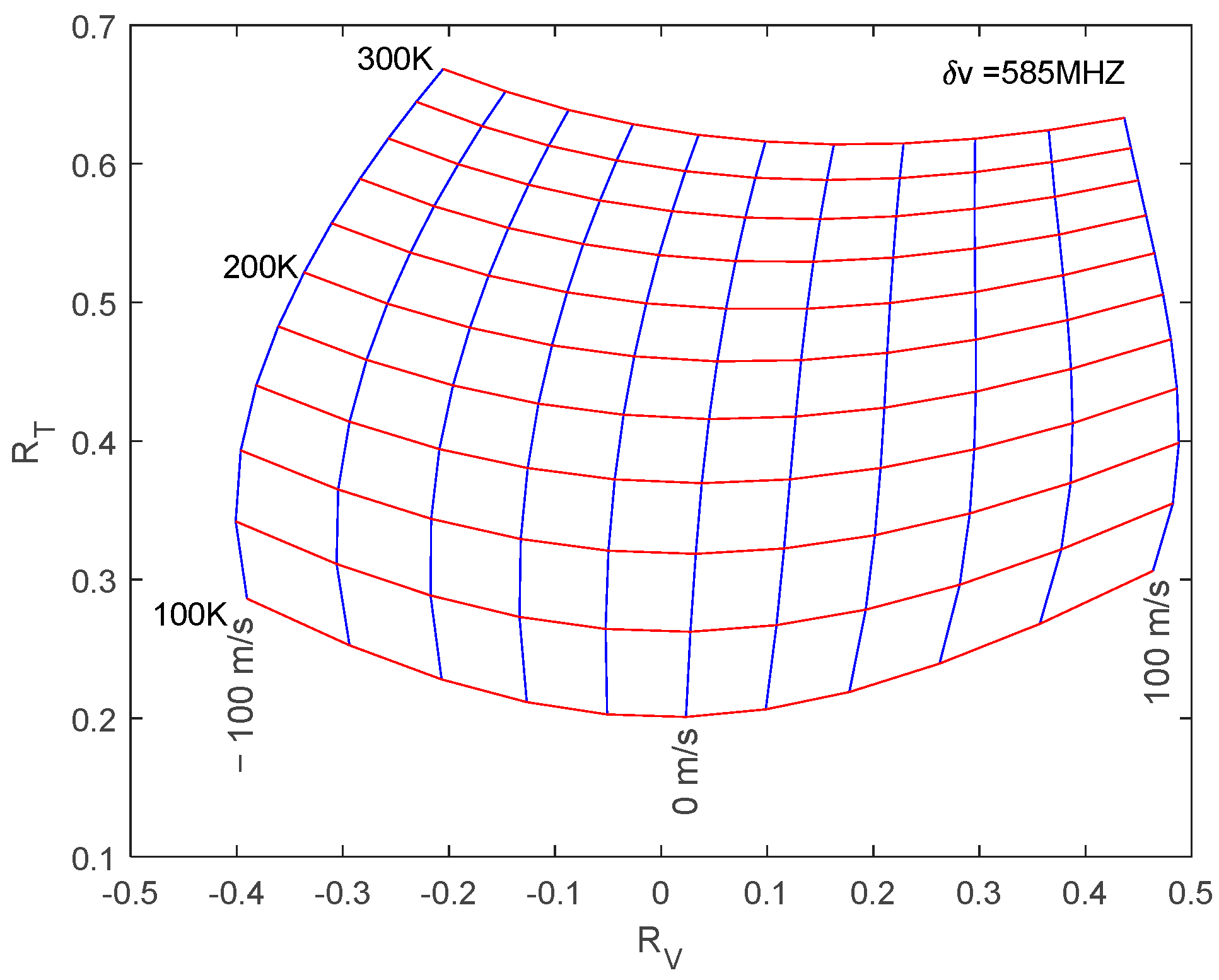
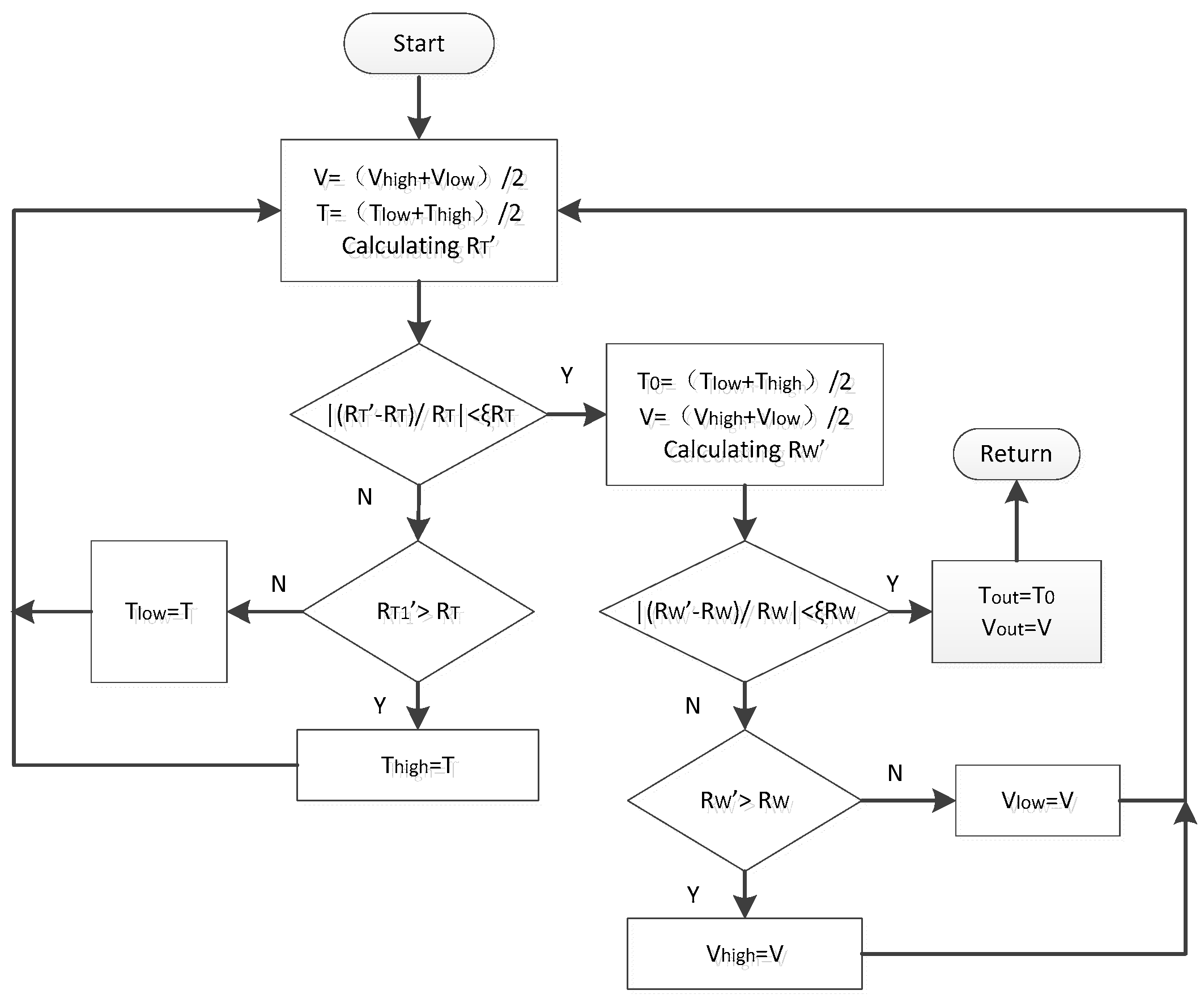
3.2.4. Iterative Retrieval of Temperature and LOS Wind

By setting the retrieval range of temperature and wind accurately, we can derive temperature and wind results more efficiently. Typically, the temperature range falls between 100 K and 300 K, and the LOS wind speed typically ranges from −150 m/s to 150 m/s in the mesopause region. We can further eliminate outliers by checking whether the RT and RV fall within their normal ranges of 0.2 < RT < 0.7 and −0.5 < RV < 0.5, as shown in Figure 1. Since both temperature and wind affect R T and R V , we can obtain corresponding values at a certain altitude by using the iterative inversion method based on Equations (1), (2), (6) and (7). We can calculate the horizontal wind (zonal and meridional wind) from the LOS wind, using the triangular geometric relationship. The flowchart in Figure 8 shows the iterative inversion steps for obtaining T and V from R T and R V . The numerical algorithm based on dichotomy involves the following basic steps:
  • Setting the retrieval range of temperature and wind. We initially set the wind speed range to −150 m/s to 150 m/s and the temperature range to 100 K to 300 K, using the initial values Tlow = 100 K, Thigh = 300 K, Vlow = −150 m/s and Vhigh = 150 m/s;
  • Using the bisection method, we decrease the range to half the previous value, refining the approximate values of temperature and wind speed until they meet the preset accuracy of ξRT and ξRW (usually set to 0.005%).

3.2.5. Synthesis of Horizontal Wind

The zonal and meridional components of wind can be obtained from the eastward and northward directions, respectively. The LOS wind speed,   v E , v N , v Z , as detected by laser beams pointed towards the east, north and zenith, can be expressed as the sum of specific components. Moreover, v E comprises the zonal wind ( μ ) and vertical wind ( w ) components along the eastward laser beam. Similarly, v N is the sum of the meridional wind ( ρ ) and vertical wind ( w ) components along the northward laser beam. With the application of simple trigonometric equations, the relationship between LOS wind and horizontal wind can be determined by Equations (10)–(12), where θ represents the zenith angle.
v Z = w
v E = μ s i n θ + w c o s θ
v N = ρ s i n θ + w c o s θ
If we assume that the atmospheric vertical wind field is zero, we can use Equations (13) and (14) to calculate the zonal and meridional wind components, respectively.
μ = v E / s i n θ
ρ = v N / s i n θ

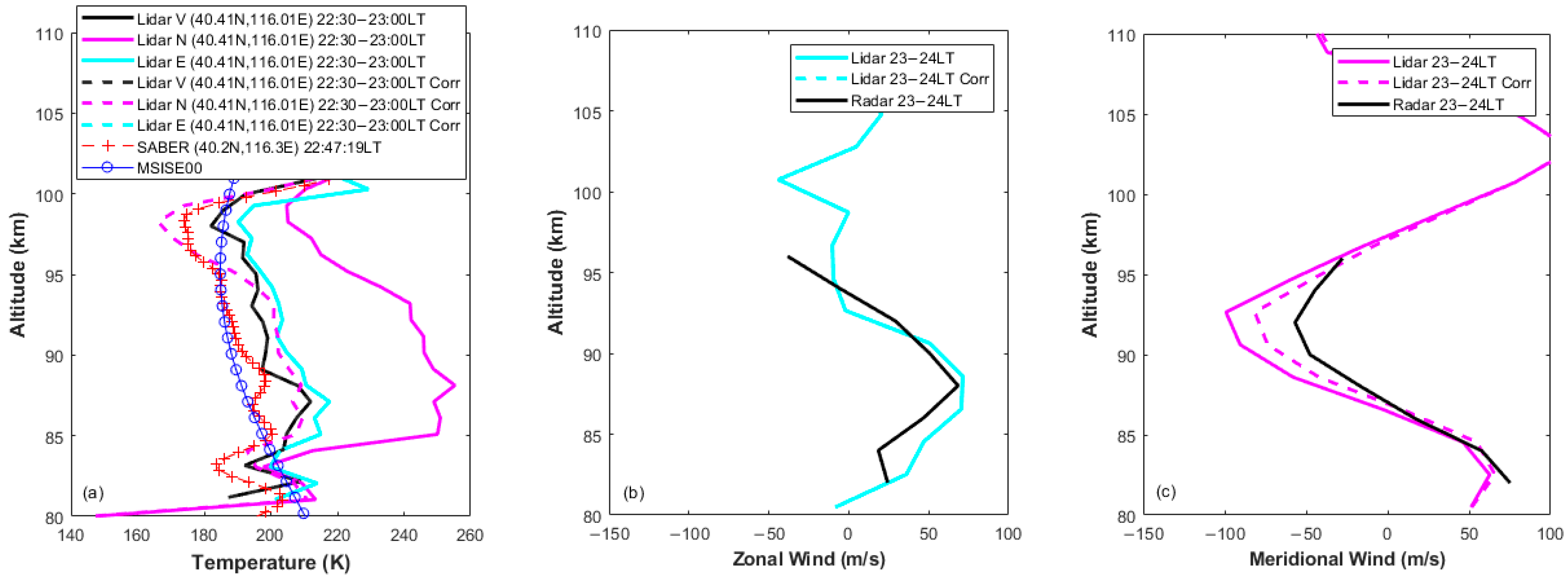
4. Observational Results and Discussion

To verify the effectiveness and feasibility of the data correction and retrieval method for diurnal observations of Na Doppler lidar, we compared the derived temperature results with those obtained from the satellite, and the horizontal winds were compared to those obtained by a nearby meteor radar. Figure 9 shows the continuous temperature results with a spatial resolution of ~2 km and temporal resolution of ~1 h, measured by the all-solid-state Na lidar on 11 December 2019. The temperature ranged between 140 and 220 K in the altitude range of 80~105 km, with obvious downward semi-diurnal tidal wave structures observed between 90 and 105 km. Figure 10 presents three examples of the temperature profiles measured by the Na lidar (the solid lines with error bars) and by the SABER (the red and gray asterisks). We selected two SABER profiles that were sampled within a range of ±6° in latitude and ±6° in longitude relative to the lidar site during the lidar valid observational period for each example. The model results from MSIS00 are also included for comparison (the blue solid lines with circles). The sampling time and the position of latitude and longitude of the satellite data are provided in each plot, respectively. The black, light blue and pink solid lines are measured by laser beams pointed towards the zenith, east and north, respectively. The error bars denoted by black short horizontal lines indicate the lidar measurement uncertainty induced by photon noise. As shown in Figure 10, the temperature-changing trends and ranges from the lidar and satellite agree well between 80 and 105 km. The lidar measurement uncertainty due to photon noise is estimated to be ~0.2 K at the sodium peak (around 90 km) and increases to over 1 K at the sodium layer edge (e.g., around 105 km), with a vertical resolution of 2 km and a temporal resolution of 1 h. Since the temporal and altitude resolutions of the temperature profiles detected by the satellite and lidar are quite different (about ~1 min and ~0.4 km for SABER and ~1 h and ~2 km for the Na lidar, respectively), and SABER uses a limb-scanning method, while the lidar is a ground-based observation whose results correspond to different altitudes at the same location. Moreover, there are also differences in the locations (longitude and latitude) between lidar and SABER samplings. The detection difference between them is within a reasonable range, though it is much larger than the measurement uncertainty of the individual profiles.
Figure 11a,b show the temporal and height variations of zonal and meridional winds measured simultaneously by the all-solid-state lidar on 11–13 December 2019. Figure 11c,d present the horizontal wind data obtained from a meteor radar (40.3°N, 116.2°E) located approximately 40 km away from the lidar station. Both the lidar and radar results have a range resolution of 2 km and a temporal resolution of 1 h. The trends observed in the lidar and radar wind results are generally consistent. Wavy structures with downward phase progressions are clearly visible in both the zonal and meridional winds. Interestingly, the meridional wind results from both the lidar and radar measurements display more pronounced semi-diurnal tidal wave structures compared to the zonal winds, even though the radar measurements suffer from a higher number of missing valid data points above 100 km. Over the course of the approximately 57-hour measurement period, the maximum meridional wind is observed at around 7 LT on 13 December in the altitude range of 84~91 km, as indicated by both the lidar and radar results. Notably, the lidar measurements reveal more intricate small-scale wave features, as the meteor radar has a larger field of view, while the lidar measures a smaller atmospheric volume.

5. Conclusions

This study investigates the method for deriving temperature and wind based on diurnal observations of the Na layer. The impact of FADOF caused by varying degrees of attenuation in the Rayleigh scattering signal and Na fluorescence signal at three different working frequencies is corrected by obtaining the FADOF attenuation correction factors from the lidar echo signals before and after inserting the FADOF. Additionally, the nonlinearity of the PMT photon counting is corrected by utilizing the input–output response curve of the PMT. These data corrections aim to avoid significant bias in measurement results, particularly around the Na layer peak. By utilizing an iterative calculation method, temperature and wind results are derived from the intensity ratios. The simultaneous temperature and wind results obtained from continuous observations using an all-solid-state Na Doppler lidar are reported for the first time. Based on a vertical resolution of 2 km and a temporal resolution of 1 h, the estimated lidar measurement uncertainty, attributed to photon noise, is approximately ±0.4 m/s for winds and ±0.2 K for temperature at around a height of 90 km (near the Na layer peak) during winter. It is worth mentioning that the uncertainties in summer are expected to be more than twice as large as those in winter due to the lower sodium abundance, which is approximately four to five times lower in summer compared to winter.
Currently, there are no other ground-based instruments near the lidar site that can measure the temperature in the mesopause region. We compared the temperature profiles retrieved by the lidar with results from SABER/TIMED. However, due to uncertainties in the SABER temperature retrievals, imperfect spatiotemporal collocation, and differences in viewing geometries between SABER and the lidar observations, it is challenging to quantitatively validate the lidar-retrieved temperature results based on individual profile comparisons. Similarly, the comparison of horizontal wind data between the lidar and nearby radar is influenced by different viewing geometries and non-common volume observations of the two instruments. Nevertheless, the overall vertical thermal structure shows similarities between the lidar and SABER temperature profiles, and there is a good overall agreement between the lidar and radar wind structures. This provides indirect evidence supporting the feasibility and rationality of the data correction and integrated data retrieval method for diurnal observations of Na Doppler lidar. However, a more comprehensive error analysis is required in future work to quantitatively assess the accuracy and reliability of the lidar retrieval.

Author Contributions

Conceptualization, X.C., F.L. and G.Y.; investigation, H.Z., Z.W., Y.X., L.D. and X.C.; formal analysis, Y.X. and Z.W.; data curation, L.D., J.W. and H.Z.; methodology, Y.X., Z.W., Y.Y. and Y.L.; resources, X.C., F.L. and G.Y.; software, Y.X., Z.W. and L.L.; validation, L.L.; writing—original draft, Y.X.; writing—review and editing, X.C., J.J., F.L. and G.Y. All authors have read and agreed to the published version of the manuscript.

Funding

This research was funded by the National Key R&D Program of China (2022YFC2807201), the Natural Science Foundation of the Jiangsu Higher Education Institutions of China (21KJB510007), the Jiangsu Province Natural Science Foundation Youth Fund Project (BK20230115), the Project supported by the Specialized Research Fund for State Key Laboratories.

Data Availability Statement

The datasets collected from the diurnal Na lidar measurements above Beijing, China, are supported by the Chinese Meridian Project (http://data.meridianproject.ac.cn/, last access: 29 June 2023). The SABER/TIMED data used in this study were downloaded from http://saber.gats-inc.com/browse_data.php (last access: 5 November 2022). The meteor radar data were supported by the Chinese Meridian Project and are available from Beijing National Observatory of Space Environment, Institute of Geology and Geophysics, Chinese Academy of Sciences, through the Geophysics Center, National Earth System Science Data Center (http://wdc.geophys.ac.cn/dbView.asp, last access: 29 June 2023).

Acknowledgments

We acknowledge the use of the data from the Chinese Meridian Project (http://data.meridianproject.ac.cn/, accessed on 29 June 2023) and the Geophysics Center, National Earth System Science Data Center. We also want to acknowledge the SABER team for making available the data used in this publication.

Conflicts of Interest

The authors declare no conflict of interest.

References

  1. Yu, B.; Xue, X.; Lu, G.; Kuo, C.; Dou, X.; Gao, Q.; Qie, X.; Wu, J.; Qiu, S.; Chi, Y.; et al. The enhancement of neutral metal Na layer above thunderstorms. Geophys. Res. Lett. 2017, 44, 9555–9563. [Google Scholar] [CrossRef]
  2. Qiu, S.; Wang, N.; Soon, W.; Lu, G.; Jia, M.; Wang, X.; Xue, X.; Li, T.; Dou, X. The sporadic sodium layer: A possible tracer for the conjunction between the upper and lower atmospheres. Atmos. Chem. Phys. 2021, 21, 11927–11940. [Google Scholar] [CrossRef]
  3. Gardner, C.S.; Kane, T.J.; Senft, D.C.; Qian, J.; Papen, G.C. Simultaneous observations of sporadic E, Na, Fe, and Caþ layers at Urbana, Illinois: Three case studies. J. Geophys. Res. 1993, 98, 16865–16873. [Google Scholar] [CrossRef]
  4. Gardner, J.A.; Viereck, R.A.; Murad, E.; Knecht, D.J.; Pike, C.P.; Broadfoot, A.L.; Anderson, E.R. Simultaneous observations of neutral and ionic magnesium in the thermosphere. Geophys. Res. Lett. 1995, 22, 2119–2122. [Google Scholar] [CrossRef]
  5. She, C.Y.; Yu, J.R. Simultaneous three-frequency Na lidar measurements of radial wind and temperature in the mesopause region. Geophys. Res. Lett. 1994, 21, 1771–1774. [Google Scholar] [CrossRef]
  6. Alpers, M.; Hoffner, J.; von Zahn, U. Iron atom densities in the polar mesosphere from lidar observations. Geophys. Res. Lett. 1990, 17, 2345–2348. [Google Scholar] [CrossRef]
  7. Alpers, M.; Höfffner, J.; von Zahn, U. Upper Atmosphere Ca and Ca+ at Mid-Latitudes: First Simultaneous and Common-Volume Lidar Observations. Geophys. Res. Lett. 1996, 23, 567–570. [Google Scholar] [CrossRef]
  8. Eska, V.; Hoffner, J.; von Zahn, U. Upper atmosphere potassium layer and its seasonal variations at 54°N. J. Geophys. Res. Space Phys. 1998, 103, 29207–29214. [Google Scholar] [CrossRef]
  9. Chu, X.Z.; Papen, G. Laser Remote Sensing: Resonance fluorescence lidar for measurements of the middle and upper atmosphere. In Book Laser Remote Sensing; Fujii, T., Fukuchi, T., Eds.; CRC Press: London, UK, 2005. [Google Scholar]
  10. Yi, F.; Zhang, S.; Yu, C.; Zhang, Y.; He, Y.; Liu, F.; Huang, K.; Huang, C.; Tan, Y. Simultaneous and common-volume three-lidar observations of sporadic metal layers in the mesopause region. J. Atmos. Sol. Terr. Phys. 2013, 102, 172–184. [Google Scholar] [CrossRef]
  11. Collins, R.L.; Li, J.; Martus, C.M. First lidar observation of the mesospheric Ni layer. Geophys. Res. Lett. 2015, 42, 665–671. [Google Scholar] [CrossRef]
  12. Dou, X.K.; Qiu, S.C.; Xue, X.H.; Chen, T.D.; Ning, B.Q. Sporadic and thermospheric enhanced sodium layers observed by a lidar chain over China. J. Geophys. Res. 2013, 118, 6627–6643. [Google Scholar] [CrossRef]
  13. Hu, X.; Yan, Z.A.; Guo, S.Y.; Cheng, Y.Q.; Gong, J.C. Sodium fluorescence Doppler lidar to measure atmospheric temperature in the mesopause region. Chin. Sci. Bull. 2011, 56, 417–423. [Google Scholar] [CrossRef]
  14. Li, T.; Fang, X.; Liu, W.; Gu, S.; Dou, X. Narrowband sodium lidar for the measurements of mesopause region temperature and wind. Appl. Opt. 2012, 51, 5401–5411. [Google Scholar] [CrossRef]
  15. Xia, Y.; Du, L.; Cheng, X.; Li, F.; Wang, J.; Wang, Z.; Yang, Y.; Lin, X.; Xun, Y.; Gong, S.; et al. Development of a solid-state sodium Doppler lidar using an all-fiber-coupled injection seeding unit for simultaneous temperature and wind measurements in the mesopause region. Opt. Express 2017, 25, 5264–5278. [Google Scholar] [CrossRef] [PubMed]
  16. Yang, Y.; Yang, Y.; Xia, Y.; Lin, X.; Zhang, L.; Jiang, H.; Cheng, X.; Liu, L.; Ji, K.; Li, F. Solid-state 589 nm seed laser based on Raman fiber amplifier for sodium wind/temperature lidar in Tibet, China. Opt. Express 2018, 26, 16226–16235. [Google Scholar] [CrossRef] [PubMed]
  17. Jiao, J.; Yang, G.; Wang, J.; Cheng, X.; Li, F.; Yang, Y.; Gong, W.; Wang, Z.; Du, L.; Yan, C.; et al. First report of sporadic K layers and comparison with sporadic Na layers at Beijing, China (40.6°N, 116.2°E). J. Geophys. Res. 2015, 120, 5214–5225. [Google Scholar] [CrossRef]
  18. Wu, F.; Zheng, H.; Cheng, X.; Yang, Y.; Li, F.; Gong, S.; Du, L.; Wang, J.; Yang, G. Simultaneous detection of the Ca and Ca+ layers by a dual-wavelength tunable lidar system. Appl. Opt. 2020, 59, 4122–4130. [Google Scholar] [CrossRef]
  19. Wu, F.; Zheng, H.; Yang, Y.; Cheng, X.; Li, F.; Du, L.; Wang, J.; Jiao, J.; Plane, J.; Feng, W.; et al. Lidar observations of the upper atmospheric Ni layer at Beijing (40°N, 116°E). J. Quant. Spec. Rad. Trans. 2021, 260, 10748. [Google Scholar] [CrossRef]
  20. Wang, C.; Chen, Z.; Xu, J. Introduction to Chinese Meridian Project—Phase II. Chin. J. Space Sci. 2020, 40, 718–722. [Google Scholar] [CrossRef]
  21. Kawahara, T.; Nozawa, S.; Saito, N.; Kawabata, T.; Tsuda, T.; Wada, S. Sodium temperature/wind lidar based on laser-diode-pumped Nd:YAG lasers deployed at Tromsø, Norway (69.6°N, 19.2°E). Opt. Express 2017, 25, 283807. [Google Scholar] [CrossRef]
  22. Krueger, D.A.; She, C.-Y.; Yuan, T. Retrieving mesopause temperature and line-of-sight wind from full-diurnal-cycle Na lidar observations. Appl. Opt. 2015, 54, 9469–9489. [Google Scholar] [CrossRef] [PubMed]
  23. Chen, H.; White, M.A.; Krueger, D.A.; She, C.Y. Daytime mesopause temperature measurements with a sodium-vapor dispersive Faraday filter in a lidar receiver. Opt. Lett. 1996, 21, 1003–1005. [Google Scholar] [CrossRef] [PubMed]
  24. Yang, Y.; Cheng, X.W.; Li, F.Q.; Hu, X.; Lin, X.; Gong, S.S. A flat spectral Faraday filter for sodium lidar. Opt. Lett. 2011, 36, 1302–1304. [Google Scholar] [CrossRef] [PubMed]
  25. Gardner, C.S.; Vargas, F.A. Optimizing three-frequency Na, Fe, and He lidars for measurements of wind, temperature, and species density and the vertical fluxes of heat and constituents. Appl. Opt. 2014, 53, 4100–4116. [Google Scholar] [CrossRef]
  26. Bills, R.E.; Gardner, C.S.; She, C. Narrowband lidar technique for sodium temperature and Doppler wind observations of the upper atmosphere. Opt. Eng. 1991, 30, 13–21. [Google Scholar] [CrossRef]
  27. Liu, A.; Guo, Y. Photomultiplier tube calibration based on Na lidar observation and its effect on heat flux bias. Appl. Opt. 2016, 55, 9467–9475. [Google Scholar] [CrossRef]
  28. Russell III, J.M.; Mlynczak, M.G.; Gordley, L.L.; Tansock, J.J.; Esplin, R. Overview of the SABER experiment and preliminary calibration results. In Proceedings of the SPIE, Optical Spectroscopic Techniques and Instrumentation for Atmospheric and Space Research III, Denver, CO, USA, 20 October 1999; Volume 3756, pp. 277–288. [Google Scholar]
  29. Dawkins, E.C.M.; Feofilov, A.; Rezac, L.; Kutepov, A.A.; Janches, D.; Höffner, J.; Chu, X.; Lu, X.; Mlynczak, M.G.; Russell, J., III. Validation of SABER v2.0 operational temperature data with ground-based lidars in the mesosphere-lower thermosphere region (75–105 km). J. Geophys. Res. Atmos. 2018, 123, 9916–9934. [Google Scholar] [CrossRef]
  30. Kutepov, A.A.; Feofilov, A.G.; Marshall, B.T.; Gordley, L.L.; Pesnell, W.D.; Goldberg, R.A.; Russell, J.M., III. SABER temperature observations in the summer polar mesosphere and lower thermosphere: Importance of accounting for the CO2v2 quanta V–V exchange. Geophys. Res. Lett. 2006, 33, L21809–L21813. [Google Scholar] [CrossRef]
  31. Feofilov, A.G.; Kutepov, A.A.; She, C.Y.; Smith, A.K.; Pesnell, W.D.; Goldberg, R.A. CO2(v2)-O quenching rate coefficient derived from coincidental SABER/TIMED and Fort Collins lidar observations of the mesosphere and lower thermosphere. Atmos. Chem. Phys. 2012, 12, 9013–9023. [Google Scholar] [CrossRef]
  32. Xia, Y.; Cheng, X.; Li, F.; Yang, Y.; Lin, X.; Jiao, J.; Du, L.; Wang, J.; Yang, G. Sodium lidar observation over full diurnal cycles in Beijing, China. Appl. Opt. 2020, 59, 1529–1536. [Google Scholar] [CrossRef]
Figure 1. Calibration curves for converting intensity ratios (RT and RV) to temperature and LOS wind (T and V), using a frequency shift amount of 585 MHz.
Remotesensing 15 05140 g001
Figure 2. The design of data acquisition program.
Remotesensing 15 05140 g002
Figure 3. Data-processing flowchart for retrieving temperature and wind.
Remotesensing 15 05140 g003
Figure 4. PMT correction curve which determines the relationship between the input and output counts of the PMT. The green line represents the theoretical correction curve for the Hamamatsu H7421-40 series PMTs, and the black line indicates a linear response plotted for reference.
Remotesensing 15 05140 g004
Figure 5. An example of raw photon count profiles (solid lines) obtained at Yanqing, Beijing, on 4 January 2022 and the corresponding profiles after PMT nonlinearity correction (dashed lines) for three laser frequencies ( v a , v + = v a + 585   M H z and v = v a 585   M H z ) from three directions (20~150 km): (a) zenith, (b) 30° off zenith to north and (c) 30° off zenith to east.
Remotesensing 15 05140 g005
Figure 6. An example of temperature and wind profiles measured by Na lidar at Yanqing, Beijing, during the night of 4 January 2022: (a) The derived temperature calculated from photon count data with 30 min integration time without (solid lines) and with (dashed lines) PMT nonlinearity correction. The temperature results from atmospheric model MSISE00 (blue circles) and TIMED/SABER (red crosses) are also included for comparison. The black, blue and pink lines represent the lidar-measured results from three directions (zenith, 30° off zenith to east and 30° off zenith to north). (b,c) Zonal and meridional wind profiles measured by Na lidar, respectively, without (blue or pink solid line) and with (blue or pink dashed line) PMT nonlinearity correction. The horizontal wind results from a nearby meteor radar are also plotted for comparison (black solid line).
Remotesensing 15 05140 g006
Figure 7. (a) An example of two adjacent photon count profiles before (solid line) and after (dashed line) inserting FADOF at v a . (b) The same as (a) but at frequency v + . (c) The same as (a) but at frequency v . (d,e) The effective transmittance through FADOF in the altitude range of 80–100 km and 30–40 km for three laser frequencies.
Remotesensing 15 05140 g007
Figure 8. The iterative retrieval steps based on the bisection method.
Remotesensing 15 05140 g008
Figure 9. Temperature measurement results obtained by Na lidar between 80 and 105 km on 11 December 2019. The temporal and spatial resolutions are ~1 h and ~2 km, respectively.
Remotesensing 15 05140 g009
Figure 10. Temperature results from lidar (solid lines with error bars), SABER (red and gray asterisks) and MSIS (blue lines with circles).
Remotesensing 15 05140 g010
Figure 11. The horizontal wind results measured by the all-solid-state Na lidar over Yanqing, Beijing (a,b), and compared with those measured by a nearby meteor radar (c,d) from ~00:00 LT on 11 December 2019 to 9 LT on 13 December 2019: (a,c) zonal wind and (b,d) meridional wind.
Remotesensing 15 05140 g011
Disclaimer/Publisher’s Note: The statements, opinions and data contained in all publications are solely those of the individual author(s) and contributor(s) and not of MDPI and/or the editor(s). MDPI and/or the editor(s) disclaim responsibility for any injury to people or property resulting from any ideas, methods, instructions or products referred to in the content.

