
Spatiotemporal Evaluation of Regional Land Use Dynamics and Its Potential Ecosystem Impact under Carbon Neutral Pathways in the Guangdong–Hong Kong–Macao Greater Bay Area
Abstract
:
1. Introduction
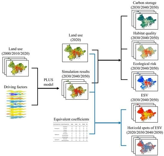
2. Materials and Methods
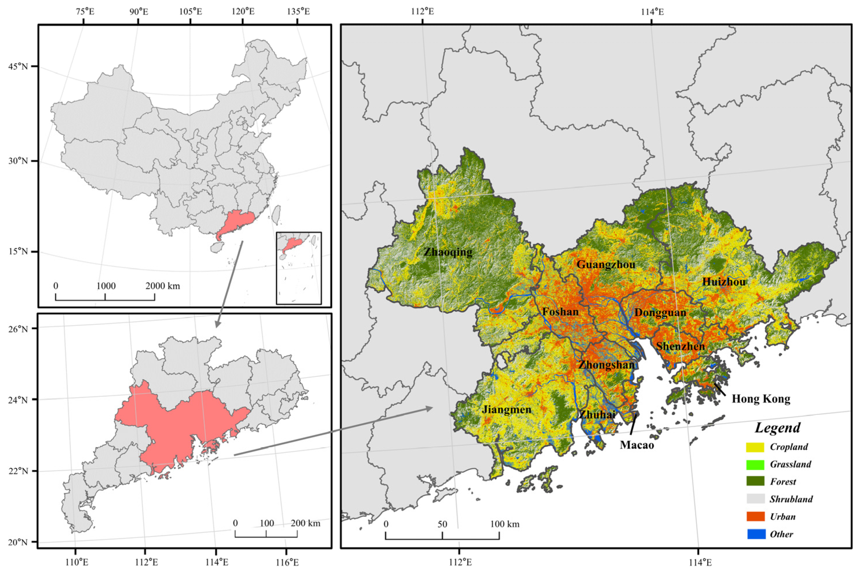
2.1. Study Area
2.2. Data Sources
2.2.1. Land-Use Data and Driving Factors
2.2.2. Statistical Data
2.3. Methodology
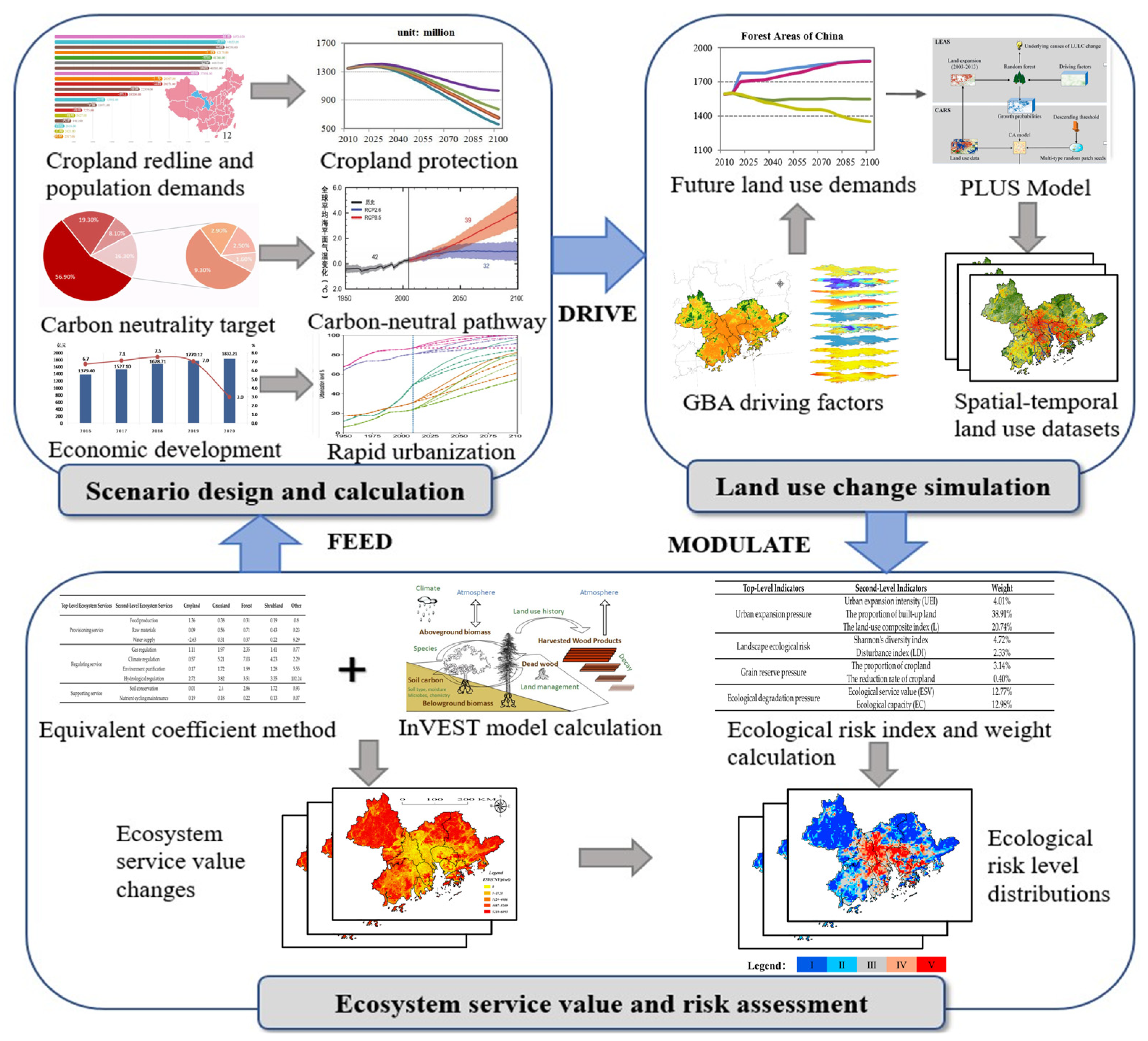
2.3.1. Land Use Change Scenario
2.3.2. Land Use Change Simulation
2.3.3. Ecosystem Service Assessment
2.3.4. Ecosystem Service Value Calculation
2.3.5. Ecological Risk Assessment
3. Results
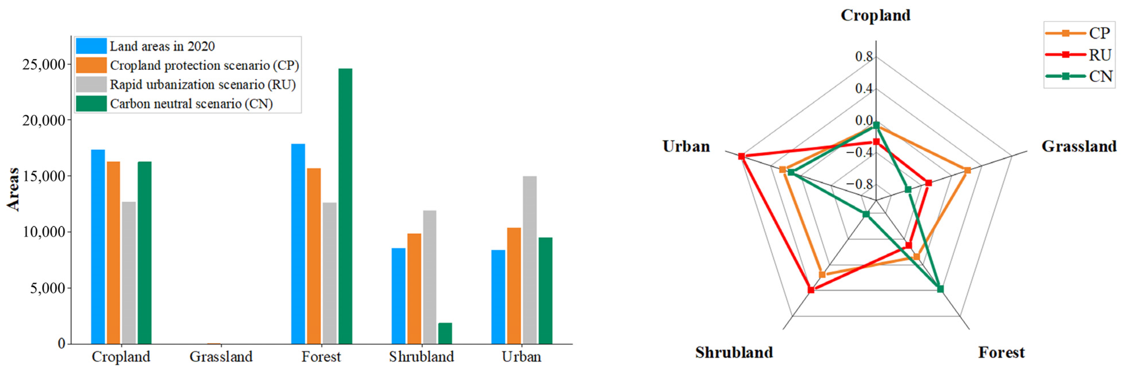
3.1. Land Use Demands under Future Scenarios
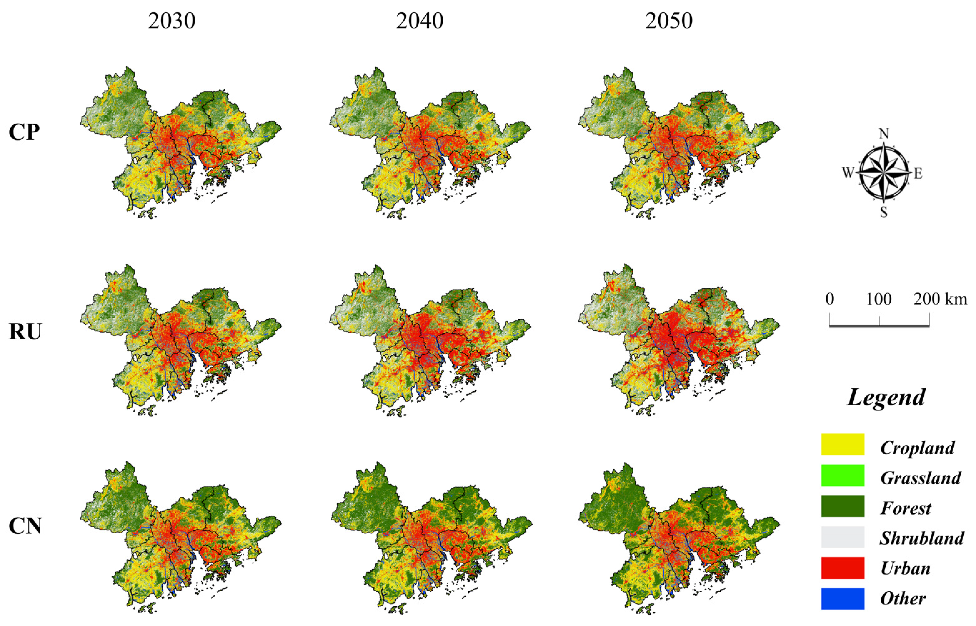
3.2. Land Use Change Simulation
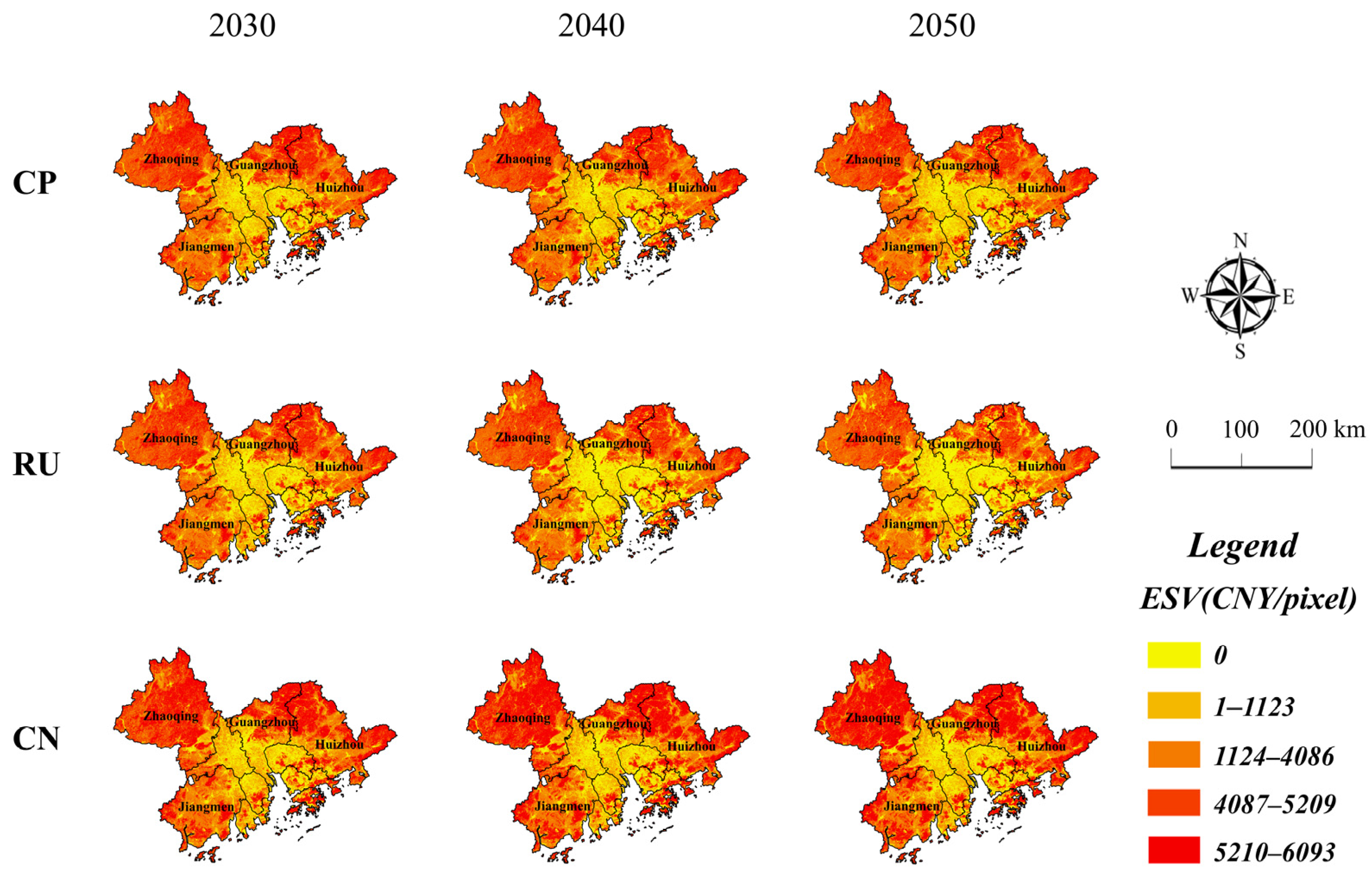
3.3. Spatial–Temporal Changes of Ecosystem Service
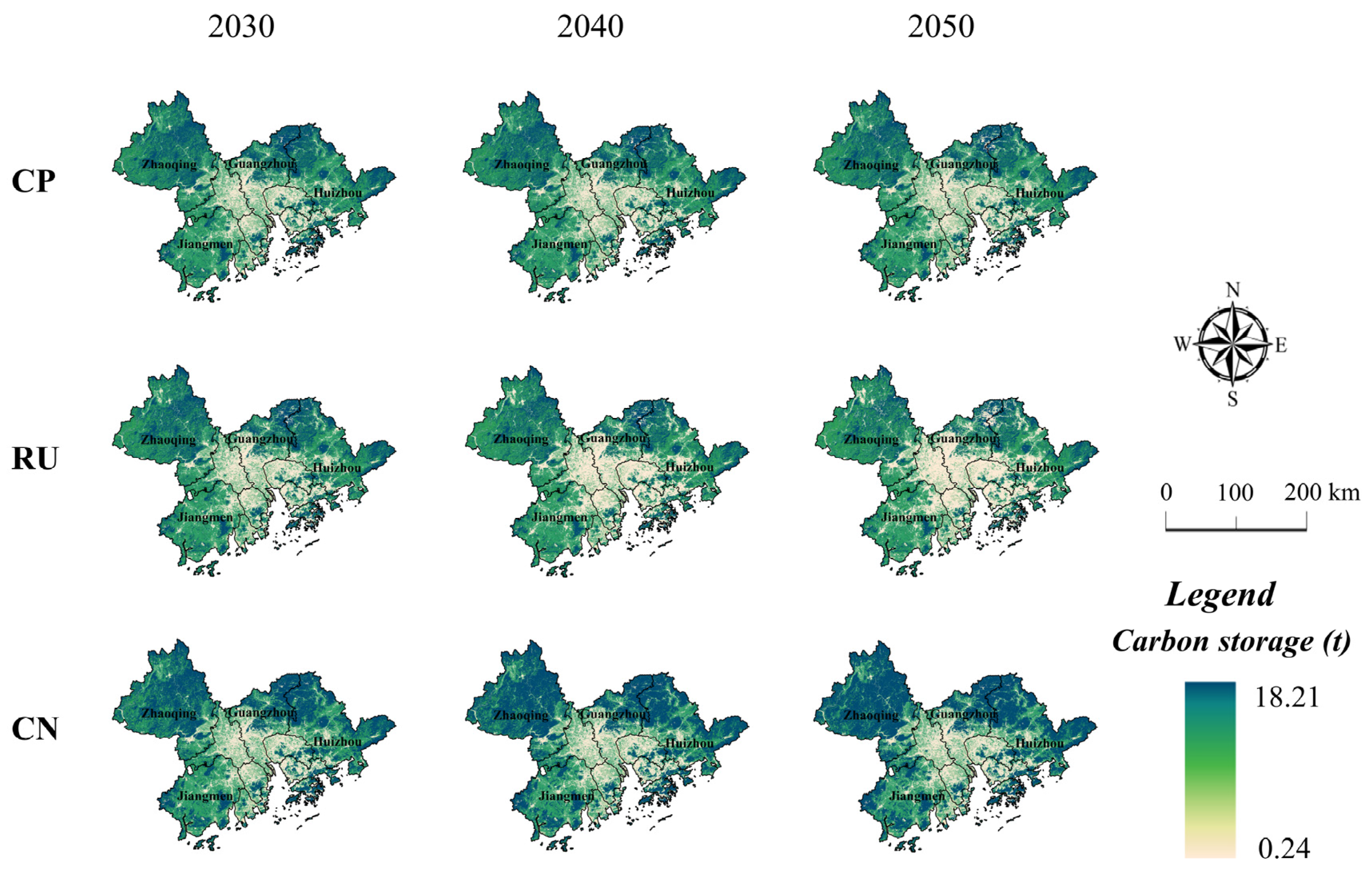
3.3.1. Carbon Storage
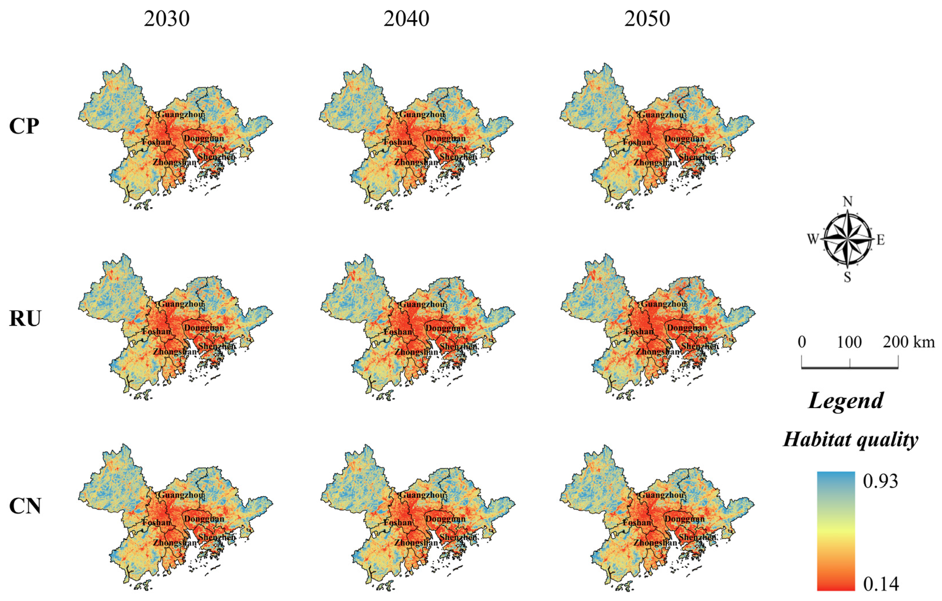
3.3.2. Habitat Quality
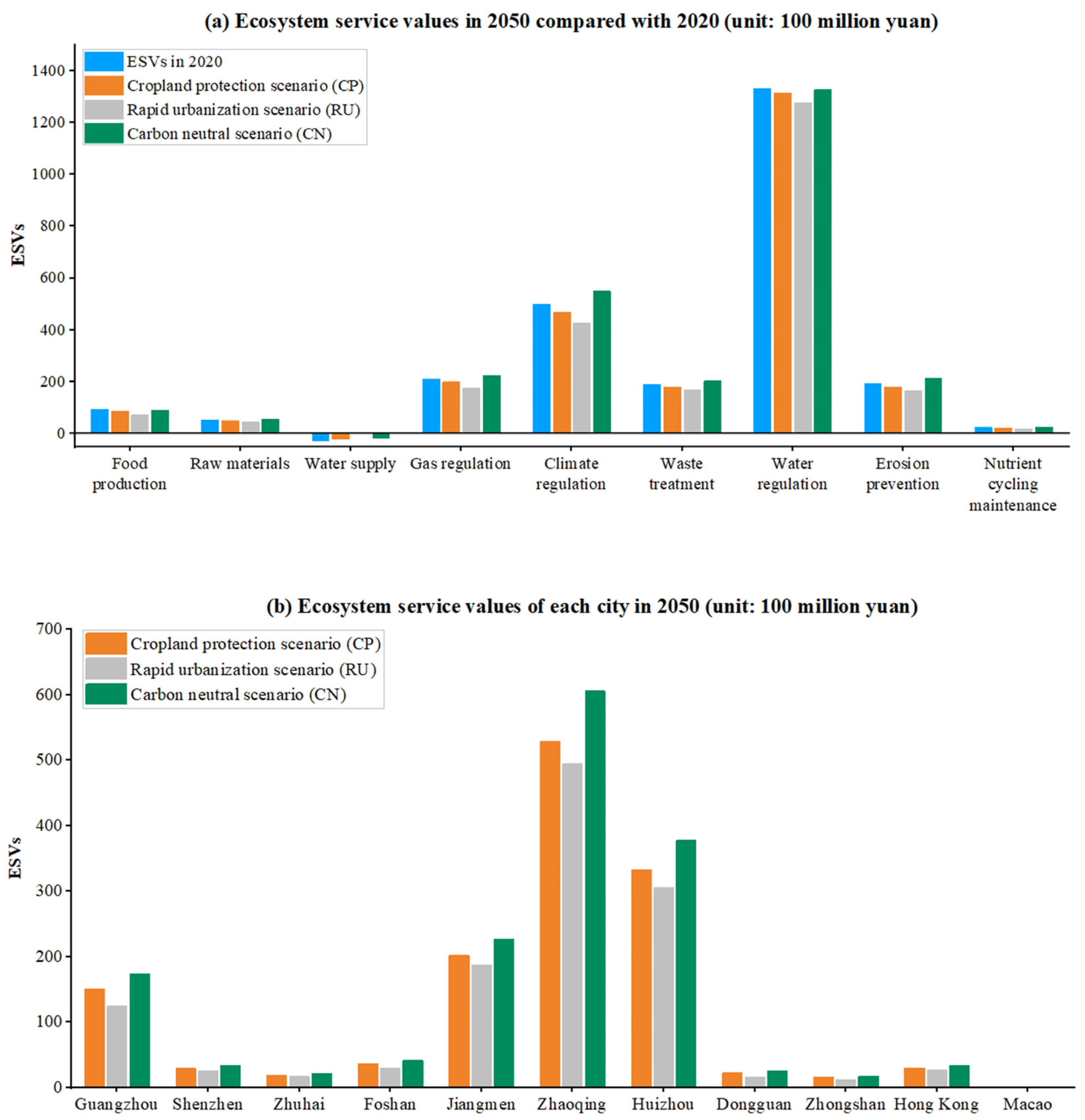
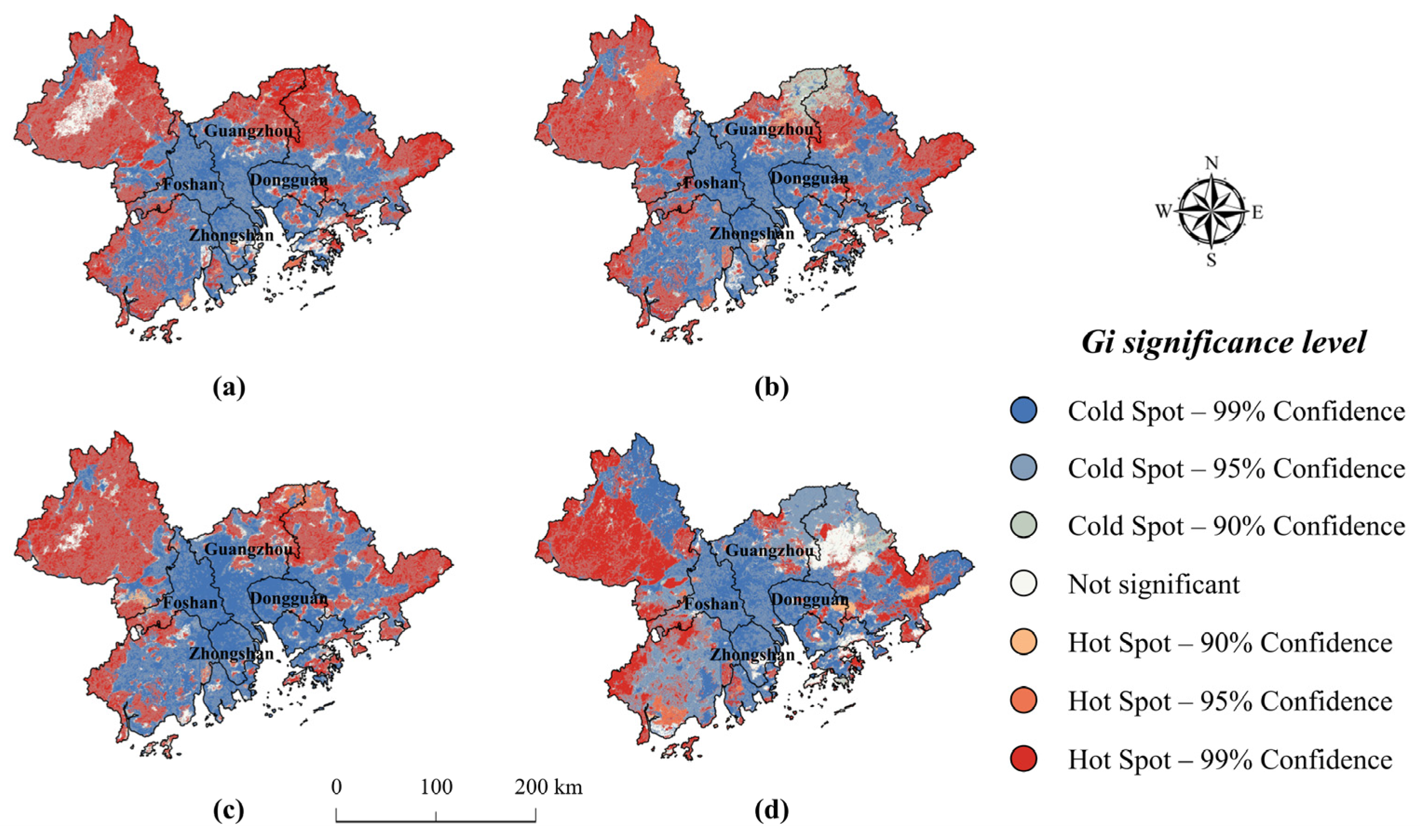
3.4. Ecosystem Service Value Changes
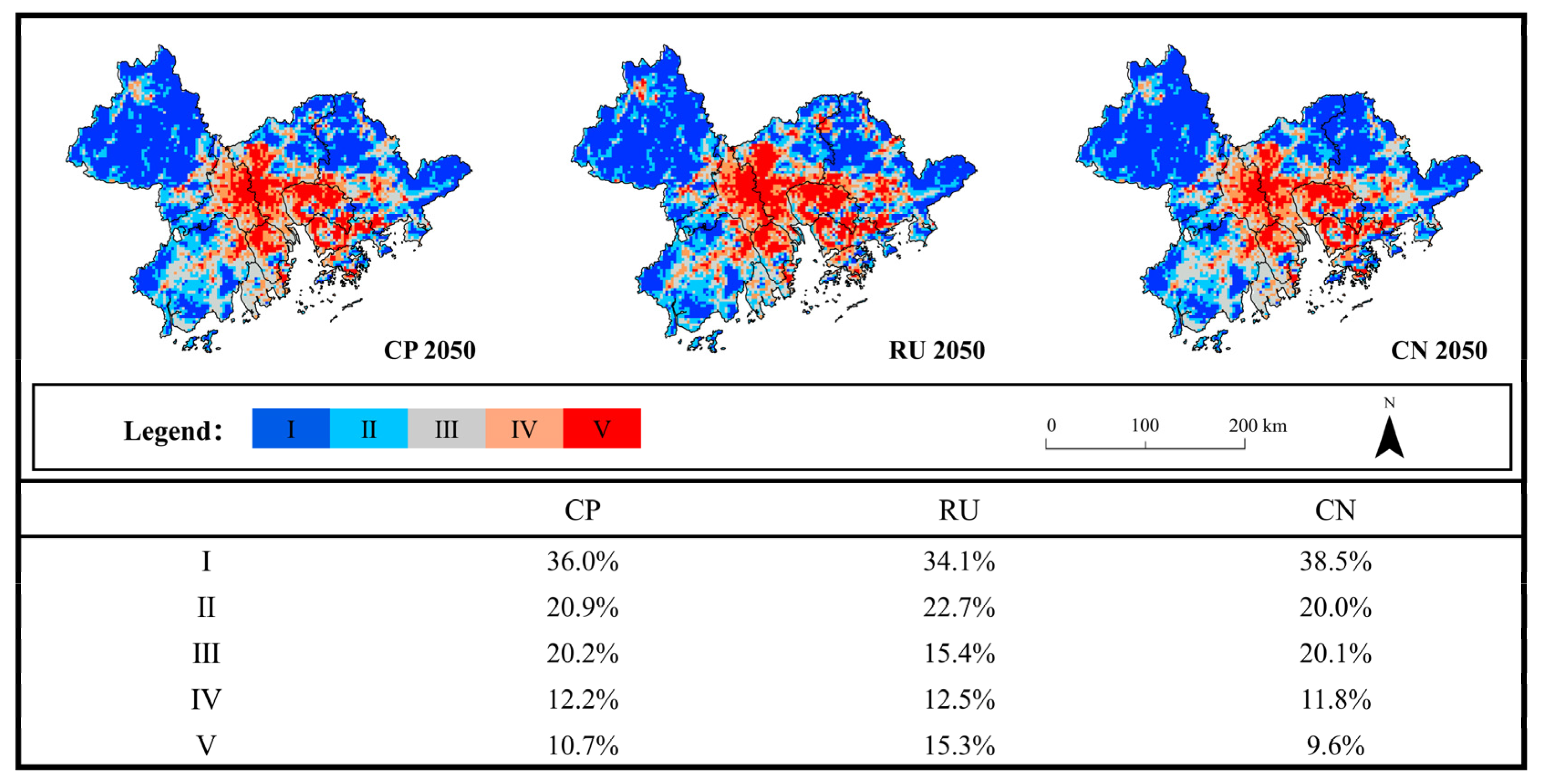
3.5. Ecological Risk Assessment
3.6. Impact of Land Use on ESV Changes
4. Discussion
4.1. Land Use Change Impact on ES and ESVs
4.2. The Relationship between Ecological Risk and LUCC
4.3. Land Use Strategies under Multiple Scenarios
5. Conclusions
- (1)
- The spatiotemporal heterogeneity of land-use patterns under different scenarios is significant. The RU scenario shows extremely high urban expansion in the central GBA at the expense of cropland and forest, which does not align with sustainable development goals. The CP scenario focuses on cropland protection. In contrast, the CN scenario has a conspicuous increase in forest area and an effective limitation in urban expansion, which is in line with the sustainable development goal.
- (2)
- Owing to the high rate of urban expansion, carbon storage and habitat quality are lower in the CP and RU scenarios, whereas they are higher in the CN scenario. The ESVs in the CP and RU scenarios are lower than in the CN scenario. The cold and hot spots of ESVs show aggregated distributions except for the CN scenario.
- (3)
- The ecological risk is closely linked to LUCC, which exhibits a higher trend in the central and southwestern GBA and lower in the northwestern and northeastern GBA. Among the three scenarios, the RU poses the highest ecological risk while the CN owns the lowest ecological risk, in which ESVs and EC rank are the top two factors, indicating a close association between LUCC and ecological risk.
- (4)
- In order to achieve carbon peaking and carbon neutrality goals, the government should formulate specific policies based on the different land-use conditions. In the central GBA, rationalizing urban expansion and strengthening the protection of ecological resources should be important tasks. In the northwestern, northeastern and southwestern GBA, it is advisable to highlight ecological carbon sequestration measures.
Supplementary Materials
Author Contributions
Funding
Data Availability Statement
Conflicts of Interest
References
- Guo, P.; Wang, H.; Qin, F.; Miao, C.; Zhang, F. Coupled MOP and PLUS-SA Model Research on Land Use Scenario Simulations in Zhengzhou Metropolitan Area, Central China. Remote Sens. 2023, 15, 3762. [Google Scholar] [CrossRef]
- Zhang, X.; Ren, W.; Peng, H. Urban land use change simulation and spatial responses of ecosystem service value under multiple scenarios: A case study of Wuhan, China. Ecol. Indic. 2022, 144, 109526. [Google Scholar] [CrossRef]
- Schirpke, U.; Tscholl, S.; Tasser, E. Spatio-temporal changes in ecosystem service values: Effects of land-use changes from past to future (1860–2100). J. Environ. Manag. 2020, 272, 111068. [Google Scholar] [CrossRef] [PubMed]
- Verburg, P.H.; Soepboer, W.; Veldkamp, A.; Limpiada, R.; Espaldon, V.; Mastura, S.S. Modeling the spatial dynamics of regional land use: The CLUE-S model. Environ. Manag. 2002, 30, 391–405. [Google Scholar] [CrossRef] [PubMed]
- Sohl, T.L.; Sayler, K.L.; Drummond, M.A.; Loveland, T.R. The FORE-SCE model: A practical approach for projecting land cover change using scenario-based modeling. J. Land Use Sci. 2007, 2, 103–126. [Google Scholar] [CrossRef]
- Liang, X.; Guan, Q.; Clarke, K.C.; Liu, S.; Wang, B.; Yao, Y. Understanding the drivers of sustainable land expansion using a patch-generating land use simulation (PLUS) model: A case study in Wuhan, China. Comput. Environ. Urban Syst. 2021, 85, 101569. [Google Scholar] [CrossRef]
- Gao, L.; Tao, F.; Liu, R.; Wang, Z.; Leng, H.; Zhou, T. Multi-scenario simulation and ecological risk analysis of land use based on the PLUS model: A case study of Nanjing. Sustain. Cities Soc. 2022, 85, 104055. [Google Scholar] [CrossRef]
- Li, C.; Wu, Y.; Gao, B.; Zheng, K.; Wu, Y.; Li, C. Multi-scenario simulation of ecosystem service value for optimization of land use in the Sichuan-Yunnan ecological barrier, China. Ecol. Indic. 2021, 132, 108328. [Google Scholar] [CrossRef]
- Grafius, D.R.; Corstanje, R.; Warren, P.H.; Evans, K.L.; Hancock, S.; Harris, J.A. The impact of land use/land cover scale on modelling urban ecosystem services. Landsc. Ecol. 2016, 31, 1509–1522. [Google Scholar] [CrossRef]
- Li, P.; Chen, J.; Li, Y.; Wu, W. Using the InVEST-PLUS Model to Predict and Analyze the Pattern of Ecosystem Carbon storage in Liaoning Province, China. Remote Sens. 2023, 15, 4050. [Google Scholar] [CrossRef]
- Li, Y.; Yao, S.; Jiang, H.; Wang, H.; Ran, Q.; Gao, X.; Ding, X.; Ge, D. Spatial-Temporal Evolution and Prediction of Carbon Storage: An Integrated Framework Based on the MOP–PLUS–InVEST Model and an Applied Case Study in Hangzhou, East China. Land 2022, 11, 2213. [Google Scholar] [CrossRef]
- Ouyang, X.; Tang, L.; Wei, X.; Li, Y. Spatial interaction between urbanization and ecosystem services in Chinese urban agglomerations. Land Use Policy 2021, 109, 105587. [Google Scholar] [CrossRef]
- Silvestri, S.; Zaibet, L.; Said, M.Y.; Kifugo, S.C. Valuing ecosystem services for conservation and development purposes: A case study from Kenya. Environ. Sci. Policy 2013, 31, 23–33. [Google Scholar] [CrossRef]
- Sun, J.; Zhang, Y.; Qin, W.; Chai, G. Estimation and simulation of forest carbon stock in northeast China forestry based on future climate change and LUCC. Remote Sens. 2022, 14, 3653. [Google Scholar] [CrossRef]
- Wang, Z.; Li, X.; Mao, Y.; Li, L.; Wang, X.; Lin, Q. Dynamic simulation of land use change and assessment of carbon storage based on climate change scenarios at the city level: A case study of Bortala, China. Ecol. Indic. 2022, 134, 108499. [Google Scholar] [CrossRef]
- Yang, W.; Jin, Y.; Sun, T.; Yang, Z.; Cai, Y.; Yi, Y. Trade-offs among ecosystem services in coastal wetlands under the effects of reclamation activities. Ecol. Indic. 2018, 92, 354–366. [Google Scholar] [CrossRef]
- Nelson, D.A. European Environment Agency. Colo. J. Int. Environ. Law Policy 1999, 10, 153. [Google Scholar]
- Hu, M.; Li, Z.; Wang, Y.; Jiao, M.; Li, M.; Xia, B. Spatio-temporal changes in ecosystem service value in response to land-use/cover changes in the Pearl River Delta. Resour. Conserv. Recycl. 2019, 149, 106–114. [Google Scholar] [CrossRef]
- Costanza, R.; d’Arge, R.; De Groot, R.; Farber, S.; Grasso, M.; Hannon, B.; Limburg, K.; Naeem, S.; O’neill, R.V.; Paruelo, J. The value of the world’s ecosystem services and natural capital. Nature 1997, 387, 253–260. [Google Scholar] [CrossRef]
- Xie, G.-D.; Lu, C.X.; Leng, Y.-F.; Zheng, D.; Li, S.J. Ecological assets valuation of the Tibetan Plateau. J. Nat. Resour. 2003, 18, 189–196. [Google Scholar] [CrossRef]
- Xie, G.; Zhang, C.; Zhen, L.; Zhang, L. Dynamic changes in the value of China’s ecosystem services. Ecosyst. Serv. 2017, 26, 146–154. [Google Scholar] [CrossRef]
- Liu, W.; Zhan, J.; Zhao, F.; Yan, H.; Zhang, F.; Wei, X. Impacts of urbanization-induced land-use changes on ecosystem services: A case study of the Pearl River Delta Metropolitan Region, China. Ecol. Indic. 2019, 98, 228–238. [Google Scholar] [CrossRef]
- Xie, Y.; Zhu, Q.; Bai, H.; Luo, P.; Liu, J. Spatio-Temporal Evolution and Coupled Coordination of LUCC and ESV in Cities of the Transition Zone, Shenmu City, China. Remote Sens. 2023, 15, 3136. [Google Scholar] [CrossRef]
- Zhang, S.; Wang, Y.; Xu, W.; Sheng, Z.; Zhu, Z.; Hou, Y. Analysis of Spatial and Temporal Variability of Ecosystem Service Values and Their Spatial Correlation in Xinjiang, China. Remote Sens. 2023, 15, 4861. [Google Scholar] [CrossRef]
- Jiang, X.; Zhai, S.; Liu, H.; Chen, J.; Zhu, Y.; Wang, Z. Multi-scenario simulation of production-living-ecological space and ecological effects based on shared socioeconomic pathways in Zhengzhou, China. Ecol. Indic. 2022, 137, 108750. [Google Scholar] [CrossRef]
- Peng, K.; Jiang, W.; Ling, Z.; Hou, P.; Deng, Y. Evaluating the potential impacts of land use changes on ecosystem service value under multiple scenarios in support of SDG reporting: A case study of the Wuhan urban agglomeration. J. Clean. Prod. 2021, 307, 127321. [Google Scholar] [CrossRef]
- Jin, X.; Jin, Y.; Mao, X. Ecological risk assessment of cities on the Tibetan Plateau based on land use/land cover changes—Case study of Delingha City. Ecol. Indic. 2019, 101, 185–191. [Google Scholar] [CrossRef]
- Xu, Q.; Guo, P.; Jin, M.; Qi, J. Multi-scenario landscape ecological risk assessment based on Markov–FLUS composite model. Geomat. Nat. Hazards Risk 2021, 12, 1449–1466. [Google Scholar] [CrossRef]
- Zhang, S.; Zhong, Q.; Cheng, D.; Xu, C.; Chang, Y.; Lin, Y.; Li, B. Landscape ecological risk projection based on the PLUS model under the localized shared socioeconomic pathways in the Fujian Delta region. Ecol. Indic. 2022, 136, 108642. [Google Scholar] [CrossRef]
- Lin, Y.; Hu, X.; Zheng, X.; Hou, X.; Zhang, Z.; Zhou, X.; Qiu, R.; Lin, J. Spatial variations in the relationships between road network and landscape ecological risks in the highest forest coverage region of China. Ecol. Indic. 2019, 96, 392–403. [Google Scholar] [CrossRef]
- Wu, J. Landscape sustainability science: Ecosystem services and human well-being in changing landscapes. Landsc. Ecol. 2013, 28, 999–1023. [Google Scholar] [CrossRef]
- Gong, J.; Yang, J.; Tang, W. Spatially explicit landscape-level ecological risks induced by land use and land cover change in a national ecologically representative region in China. Int. J. Environ. Res. Public Health 2015, 12, 14192–14215. [Google Scholar] [CrossRef] [PubMed]
- Jiang, M.; Chen, H.; Chen, Q. A method to analyze “source–sink” structure of non-point source pollution based on remote sensing technology. Environ. Pollut. 2013, 182, 135–140. [Google Scholar] [CrossRef] [PubMed]
- Liu, Y.; Liu, Y.; Li, J.; Lu, W.; Wei, X.; Sun, C. Evolution of landscape ecological risk at the optimal scale: A case study of the open coastal wetlands in Jiangsu, China. Int. J. Environ. Res. Public Health 2018, 15, 1691. [Google Scholar] [CrossRef] [PubMed]
- Yan, Z.; Wang, Y.; Wang, Z.; Zhang, C.; Wang, Y.; Li, Y. Spatiotemporal Analysis of Landscape Ecological Risk and Driving Factors: A Case Study in the Three Gorges Reservoir Area, China. Remote Sens. 2023, 15, 4884. [Google Scholar] [CrossRef]
- Cui, L.; Zhao, Y.; Liu, J.; Han, L.; Ao, Y.; Yin, S. Landscape ecological risk assessment in Qinling Mountain. Geol. J. 2018, 53, 342–351. [Google Scholar] [CrossRef]
- Li, W.; Wang, Y.; Xie, S.; Sun, R.; Cheng, X. Impacts of landscape multifunctionality change on landscape ecological risk in a megacity, China: A case study of Beijing. Ecol. Indic. 2020, 117, 106681. [Google Scholar] [CrossRef]
- Wang, B.; Ding, M.; Li, S.; Liu, L.; Ai, J. Assessment of landscape ecological risk for a cross-border basin: A case study of the Koshi River Basin, central Himalayas. Ecol. Indic. 2020, 117, 106621. [Google Scholar] [CrossRef]
- Xu, W.; Wang, J.; Zhang, M.; Li, S. Construction of landscape ecological network based on landscape ecological risk assessment in a large-scale opencast coal mine area. J. Clean. Prod. 2021, 286, 125523. [Google Scholar] [CrossRef]
- Venkatesh, K.; John, R.; Chen, J.; Xiao, J.; Amirkhiz, R.G.; Giannico, V.; Kussainova, M. Optimal ranges of social-environmental drivers and their impacts on vegetation dynamics in Kazakhstan. Sci. Total Environ. 2022, 847, 157562. [Google Scholar] [CrossRef]
- Zheng, K.; Tan, L.; Sun, Y.; Wu, Y.; Duan, Z.; Xu, Y.; Gao, C. Impacts of climate change and anthropogenic activities on vegetation change: Evidence from typical areas in China. Ecol. Indic. 2021, 126, 107648. [Google Scholar] [CrossRef]
- Zhang, X.; Liu, L.; Chen, X.; Gao, Y.; Xie, S.; Mi, J. GLC_FCS30: Global land-cover product with fine classification system at 30 m using time-series Landsat imagery. Earth Syst. Sci. Data 2021, 13, 2753–2776. [Google Scholar] [CrossRef]
- Wu, P.; Liu, X.; Li, X.; Chen, Y. Impact of urban expansion on carbon storage in terrestrial ecosystems based on InVEST model and CA: A case study of Guangdong Province. Geogr. Geo-Inf. Sci. 2016, 32, 22–28. [Google Scholar] [CrossRef]
- Terrado, M.; Sabater, S.; Chaplin-Kramer, B.; Mandle, L.; Ziv, G.; Acuña, V. Model development for the assessment of terrestrial and aquatic habitat quality in conservation planning. Sci. Total Environ. 2016, 540, 63–70. [Google Scholar] [CrossRef] [PubMed]
- Huang, Y.; Sun, W.; Qin, Z.; Zhang, W.; Yu, Y.; Li, T.; Zhang, Q.; Wang, G.; Yu, L.; Wang, Y. The role of China’s terrestrial carbon sequestration 2010–2060 in offsetting energy-related CO2 emissions. Natl. Sci. Rev. 2022, 9, nwac057. [Google Scholar] [CrossRef] [PubMed]
- Andersson, E.; Langemeyer, J.; Borgstrom, S.; McPhearson, T.; Haase, D.; Kronenberg, J.; Barton, D.N.; Davis, M.; Naumann, S.; Roschel, L.; et al. Enabling Green and Blue Infrastructure to Improve Contributions to Human Well-Being and Equity in Urban Systems. Bioscience 2019, 69, 566–574. [Google Scholar] [CrossRef] [PubMed]
- Nelson, E.; Mendoza, G.; Regetz, J.; Polasky, S.; Tallis, H.; Cameron, D.; Chan, K.M.; Daily, G.C.; Goldstein, J.; Kareiva, P.M. Modeling multiple ecosystem services, biodiversity conservation, commodity production, and tradeoffs at landscape scales. Front. Ecol. Environ. 2009, 7, 4–11. [Google Scholar] [CrossRef]
- Xie, G.; Zhang, C.-X.; Zhang, L.-M.; Chen, W.; Li, S. Improvement of the evaluation method for ecosystem service value based on per unit area. J. Nat. Resour. 2015, 30, 1243. [Google Scholar] [CrossRef]
- Ge, G.; Zhang, J.; Chen, X.; Liu, X.; Hao, Y.; Yang, X.; Kwon, S. Effects of land use and land cover change on ecosystem services in an arid desert-oasis ecotone along the Yellow River of China. Ecol. Eng. 2022, 176, 106512. [Google Scholar] [CrossRef]
- Zhao, Q.; Wen, Z.; Chen, S.; Ding, S.; Zhang, M. Quantifying land use/land cover and landscape pattern changes and impacts on ecosystem services. Int. J. Environ. Res. Public Health 2020, 17, 126. [Google Scholar] [CrossRef]
- Li, G.; Fang, C.; Wang, S. Exploring spatiotemporal changes in ecosystem-service values and hotspots in China. Sci. Total Environ. 2016, 545, 609–620. [Google Scholar] [CrossRef] [PubMed]
- Su, L.; Fan, J.; Fu, L. Exploration of smart city construction under new urbanization: A case study of Jinzhou-Huludao Coastal Area. Sustain. Comput. Inform. Syst. 2020, 27, 100403. [Google Scholar] [CrossRef]
- Han, Z.; Li, J.; Yin, H.; Shen, T.Y.J.; Xu, C. Analysis of ecological security of wetland in Liaohe River delta based on the landscape pattern. Ecol. Environ. Sci. 2010, 19, 701–705. [Google Scholar]
- Guo, H.; Dong, S.; Wu, D.; Pei, S.; Xin, X. Calculation and analysis of equivalence factor and yield factor of ecological footprint based on ecosystem services value. Acta Ecol. Sin. 2020, 40, 1405–1412. [Google Scholar] [CrossRef]
- Zou, Z.-H.; Yi, Y.; Sun, J.-N. Entropy method for determination of weight of evaluating indicators in fuzzy synthetic evaluation for water quality assessment. J. Environ. Sci. 2006, 18, 1020–1023. [Google Scholar] [CrossRef] [PubMed]
- Li, Y.; Liu, W.; Feng, Q.; Zhu, M.; Yang, L.; Zhang, J.; Yin, X. The role of land use change in affecting ecosystem services and the ecological security pattern of the Hexi Regions, Northwest China. Sci. Total Environ. 2023, 855, 158940. [Google Scholar] [CrossRef] [PubMed]
- Zhu, G.; Qiu, D.; Zhang, Z.; Sang, L.; Liu, Y.; Wang, L.; Zhao, K.; Ma, H.; Xu, Y.; Wan, Q. Land-use changes lead to a decrease in carbon storage in arid region, China. Ecol. Indic. 2021, 127, 107770. [Google Scholar] [CrossRef]
- Fahey, T.J.; Woodbury, P.B.; Battles, J.J.; Goodale, C.L.; Hamburg, S.P.; Ollinger, S.V.; Woodall, C.W. Forest carbon storage: Ecology, management, and policy. Front. Ecol. Environ. 2010, 8, 245–252. [Google Scholar] [CrossRef]
- Song, Y.; Chen, B.; Kwan, M.-P. How does urban expansion impact people’s exposure to green environments? A comparative study of 290 Chinese cities. J. Clean. Prod. 2020, 246, 119018. [Google Scholar] [CrossRef]
- Fan, F.; Xiao, C.; Feng, Z.; Chen, Y. Land-planning management based on multiple ecosystem services and simulation in tropical forests. J Environ. Manag. 2022, 323, 116216. [Google Scholar] [CrossRef]
- Huang, A.; Xu, Y.; Sun, P.; Zhou, G.; Liu, C.; Lu, L.; Xiang, Y.; Wang, H. Land use/land cover changes and its impact on ecosystem services in ecologically fragile zone: A case study of Zhangjiakou City, Hebei Province, China. Ecol. Indic. 2019, 104, 604–614. [Google Scholar] [CrossRef]
- Liang, Y.; Song, W. Integrating potential ecosystem services losses into ecological risk assessment of land use changes: A case study on the Qinghai-Tibet Plateau. J. Environ. Manag. 2022, 318, 115607. [Google Scholar] [CrossRef] [PubMed]
- Li, J.; Guo, X.; Chuai, X.; Xie, F.; Yang, F.; Gao, R.; Ji, X. Reexamine China’s terrestrial ecosystem carbon balance under land use-type and climate change. Land Use Policy 2021, 102, 105275. [Google Scholar] [CrossRef]
- Li, J.; Ouyang, X.; Zhu, X. Land space simulation of urban agglomerations from the perspective of the symbiosis of urban development and ecological protection: A case study of Changsha-Zhuzhou-Xiangtan urban agglomeration. Ecol. Indic. 2021, 126, 107669. [Google Scholar] [CrossRef]
- Li, M.; Liang, D.; Xia, J.; Song, J.; Cheng, D.; Wu, J.; Cao, Y.; Sun, H.; Li, Q. Evaluation of water conservation function of Danjiang River Basin in Qinling Mountains, China based on InVEST model. J. Environ. Manag. 2021, 286, 112212. [Google Scholar] [CrossRef] [PubMed]
- Cao, Y.; Kong, L.; Zhang, L.; Ouyang, Z. The balance between economic development and ecosystem service value in the process of land urbanization: A case study of China’s land urbanization from 2000 to 2015. Land Use Policy 2021, 108, 105536. [Google Scholar] [CrossRef]
- Fang, Z.; Ding, T.; Chen, J.; Xue, S.; Zhou, Q.; Wang, Y.; Wang, Y.; Huang, Z.; Yang, S. Impacts of land use/land cover changes on ecosystem services in ecologically fragile regions. Sci. Total Environ. 2022, 831, 154967. [Google Scholar] [CrossRef] [PubMed]
- Ma, Q. Integrating ecological correlation into cellular automata for urban growth simulation: A case study of Hangzhou, China. Urban For. Urban Green. 2020, 51, 126697. [Google Scholar] [CrossRef]


| Research | Land Use Change Scenario | Region | Ecological Service Value Assessment | Ecological Risk Assessment |
|---|---|---|---|---|
| Hu et al. [18] | Historical | the Pearl River Delta (PRD) | the equivalent coefficients table method | / |
| Liu et al. [22] | Historical | the PRD | ||
| Schirpke et al. [3] | Business as usual scenario, ‘Liberalization’ scenario, ‘Rewilding’ scenario, ‘Food sovereignty’ scenario | South Tyrol, Italy | derived from the ES supply, and was weighted by the socio-cultural preference values | |
| Jiang et al. [25] | SSP1, SSP2, SSP3, SSP4, SSP5 | Zhengzhou | eco-environmental quality index, ecological contribution rate of land use transition | |
| Peng et al. [26] | Natural increase scenario, economic development scenario, ecological protection scenario | Wuhan | the equivalent coefficients table method | |
| Zhang et al. [2] | Natural development scenario, cultivated land protection scenario, ecological protection scenario, urban development scenario | Wuhan | ||
| Jin et al. [27] | Historical | Delingha city | / | land use types, the loss index of each land use type |
| Xu et al. [28] | Natural growth scenario, ecological protection scenario | Xinjiang | landscape loss index, ecological sensitivity index | |
| Zhang et al. [29] | SSP1, SSP2, SSP3, SSP4, SSP5 | Fujian Delta region | landscape disturbance index, the landscape vulnerability index, and land use types | |
| Gao et al. [7] | BAU scenario, RED scenario (maximum economic benefit), ELP scenario (maximize the ecological benefit) | Nanjing | the equivalent coefficients table method | urban expansion pressure, landscape ecological risk, grain reserve pressure, ecological degradation pressure |
| Top-Level Ecosystem Services | Second-Level Ecosystem Services | Cropland | Grassland | Forest | Shrubland | Other |
|---|---|---|---|---|---|---|
| Provisioning service | Food production | 1.36 | 0.38 | 0.31 | 0.19 | 0.8 |
| Raw materials | 0.09 | 0.56 | 0.71 | 0.43 | 0.23 | |
| Water supply | −2.63 | 0.31 | 0.37 | 0.22 | 8.29 | |
| Regulating service | Gas regulation | 1.11 | 1.97 | 2.35 | 1.41 | 0.77 |
| Climate regulation | 0.57 | 5.21 | 7.03 | 4.23 | 2.29 | |
| Environment purification | 0.17 | 1.72 | 1.99 | 1.28 | 5.55 | |
| Hydrological regulation | 2.72 | 3.82 | 3.51 | 3.35 | 102.24 | |
| Supporting service | Soil conservation | 0.01 | 2.4 | 2.86 | 1.72 | 0.93 |
| Nutrient cycling maintenance | 0.19 | 0.18 | 0.22 | 0.13 | 0.07 |
| Top-Level Indicators | Second-Level Indicators | Weight |
|---|---|---|
| Urban expansion pressure | Urban expansion intensity (UEI) | 4.01% |
| The proportion of built-up land | 38.91% | |
| The land-use composite index (L) | 20.74% | |
| Landscape ecological risk | Shannon’s diversity index | 4.72% |
| Disturbance index (LDI) | 2.33% | |
| Grain reserve pressure | The proportion of cropland | 3.14% |
| The reduction rate of cropland | 0.40% | |
| Ecological degradation pressure | Ecosystem service value (ESV) | 12.77% |
| Ecological capacity (EC) | 12.98% |
| Scenario | Year | Cropland | Grassland | Forest | Shrubland | Urban | Other |
|---|---|---|---|---|---|---|---|
| / | 2020 | 31.247% | 0.011% | 32.228% | 15.395% | 15.110% | 6.008% |
| CP | 2030 | 30.577% | 0.011% | 30.725% | 16.802% | 15.878% | 6.008% |
| 2040 | 29.921% | 0.012% | 29.244% | 17.667% | 17.149% | 6.008% | |
| 2050 | 29.279% | 0.013% | 28.228% | 17.766% | 18.704% | 6.008% | |
| RU | 2030 | 28.695% | 0.012% | 28.793% | 17.819% | 18.673% | 6.008% |
| 2040 | 25.928% | 0.011% | 25.161% | 19.814% | 23.077% | 6.008% | |
| 2050 | 22.832% | 0.008% | 22.712% | 21.447% | 26.994% | 6.008% | |
| CN | 2030 | 30.577% | 0.008% | 37.009% | 10.632% | 15.766% | 6.008% |
| 2040 | 29.921% | 0.006% | 41.789% | 5.855% | 16.422% | 6.008% | |
| 2050 | 29.279% | 0.005% | 44.313% | 3.317% | 17.078% | 6.008% |
| Scenario | Year | Cropland | Grassland | Forest | Shrubland | Urban | Other |
|---|---|---|---|---|---|---|---|
| / | 2020 | 202,038,233 | 94,873 | 287,357,803 | 87,725,762 | 1,742,112 | 3,823,298 |
| CP | 2030 | 197,704,969 | 93,458 | 273,953,927 | 95,739,005 | 1,830,582 | 3,823,298 |
| 2040 | 193,464,649 | 98,753 | 260,748,807 | 100,667,960 | 1,977,139 | 3,823,298 | |
| 2050 | 189,315,280 | 115,197 | 251,693,685 | 101,235,551 | 2,156,509 | 3,823,298 | |
| RU | 2030 | 185,535,153 | 99,137 | 256,733,535 | 101,534,104 | 2,152,920 | 3,823,298 |
| 2040 | 167,643,701 | 98,124 | 224,349,632 | 112,906,215 | 2,660,603 | 3,823,298 | |
| 2050 | 147,628,789 | 66,039 | 202,505,588 | 122,206,343 | 3,112,205 | 3,823,298 | |
| CN | 2030 | 197,704,890 | 65,445 | 329,986,965 | 60,583,983 | 1,817,733 | 3,823,298 |
| 2040 | 193,464,570 | 48,092 | 372,603,634 | 33,360,121 | 1,893,355 | 3,823,298 | |
| 2050 | 189,315,280 | 40,298 | 395,114,261 | 18,898,717 | 1,968,977 | 3,823,298 |
Disclaimer/Publisher’s Note: The statements, opinions and data contained in all publications are solely those of the individual author(s) and contributor(s) and not of MDPI and/or the editor(s). MDPI and/or the editor(s) disclaim responsibility for any injury to people or property resulting from any ideas, methods, instructions or products referred to in the content. |
© 2023 by the authors. Licensee MDPI, Basel, Switzerland. This article is an open access article distributed under the terms and conditions of the Creative Commons Attribution (CC BY) license (https://creativecommons.org/licenses/by/4.0/).
Share and Cite
Chen, H.; Dong, N.; Liang, X.; Huang, H. Spatiotemporal Evaluation of Regional Land Use Dynamics and Its Potential Ecosystem Impact under Carbon Neutral Pathways in the Guangdong–Hong Kong–Macao Greater Bay Area. Remote Sens. 2023, 15, 5749. https://doi.org/10.3390/rs15245749
Chen H, Dong N, Liang X, Huang H. Spatiotemporal Evaluation of Regional Land Use Dynamics and Its Potential Ecosystem Impact under Carbon Neutral Pathways in the Guangdong–Hong Kong–Macao Greater Bay Area. Remote Sensing. 2023; 15(24):5749. https://doi.org/10.3390/rs15245749
Chicago/Turabian StyleChen, Haoming, Na Dong, Xun Liang, and Huabing Huang. 2023. "Spatiotemporal Evaluation of Regional Land Use Dynamics and Its Potential Ecosystem Impact under Carbon Neutral Pathways in the Guangdong–Hong Kong–Macao Greater Bay Area" Remote Sensing 15, no. 24: 5749. https://doi.org/10.3390/rs15245749