
A Multi-Level Auto-Adaptive Noise-Filtering Algorithm for Land ICESat-2 Photon-Counting Data

1
College of Urban Railway Transportation, Shanghai University of Engineering Science, Shanghai 201620, China
2
Shanghai Key Laboratory for Planetary Mapping and Remote Sensing for Deep Space Exploration, College of Surveying and Geo-Informatics, Tongji University, Shanghai 200092, China
3
College of Environmental Science and Engineering, Donghua University, Shanghai 201620, China
*
Author to whom correspondence should be addressed.
Remote Sens. 2023, 15(21), 5176; https://doi.org/10.3390/rs15215176
Submission received: 28 August 2023
/
Revised: 16 October 2023
/
Accepted: 26 October 2023
/
Published: 30 October 2023
(This article belongs to the Special Issue Multi-Platform Remote Sensing for the Modeling and Analysis of Smart Cities)
Abstract
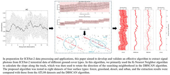
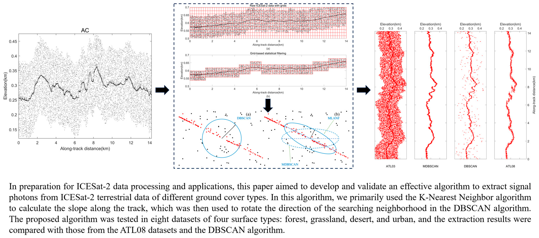
:Due to atmospheric scattering, solar radiation, and other factors, the Ice, Cloud, and land Elevation Satellite-2 (ICESat-2) product data suffer from a substantial amount of background noise. This poses a significant challenge when attempting to directly utilize the raw data. Consequently, data denoising becomes an indispensable preprocessing step for its subsequent applications, such as the extraction of forest structure parameters and ground elevation data. While the Density-Based Spatial Clustering of Applications with Noise (DBSCAN) algorithm is currently the most widely used method, it remains susceptible to complexities arising from terrain, low signal-to-noise ratio (SNR), and input parameter variations. This paper proposes an efficient Multi-Level Auto-Adaptive Noise Filter (MLANF) algorithm based on photon spatial density. Its purpose is to extract signal photons from ICESat-2 terrestrial data of different ground cover types. The algorithm follows a two-step process. Firstly, random noise photons are removed from the upper and lower regions of the signal photons through a coarse denoising process. Secondly, in the fine denoising step, the K-Nearest Neighbor (KNN) algorithm selects the K photons to calculate the slope along the track. The calculated slope is then used to rotate the direction of the searching neighborhood in the DBSCAN algorithm. The proposed algorithm was tested in eight datasets of four surface types: forest, grassland, desert, and urban, and the extraction results were compared with those from the ATL08 datasets and the DBSCAN algorithm. Based on the ground-truth signal photons obtained by visual inspection, the classification precision, recall, and F-score of our algorithm, as well as two other algorithms, were calculated. The MLANF could achieve a good balance between classification precision (97.48% averaged) and recall (97.96% averaged). Its F-score (97.69% averaged) was higher than that of the other two methods. This demonstrates that the MLANF algorithm successfully obtained a continuous surface profile from ICESat-2 datasets with different surface cover types, significant topographic relief, and low SNR.
1. Introduction
Due to the rapid development of laser technology, high-precision laser sensors become increasingly important in data acquisition across various fields. Most laser detection techniques have a limited scanning range due to the short sensing distance of the sensor. In addition, large-scale observations and applications are expensive. The emergence of satellite-based LiDAR technology resolves these limitations. In September 2018 [1], the Advanced Topography Laser Altimeter System (ATLAS) with the single-photon laser altimeter ICESat-2 was successfully launched. This new type of laser detection technology could cover a sufficiently wide area [2,3,4]. In the ATLAS, the transmit laser pulse is split into three pairs of beams to improve the data acquisition efficiency. Each pair consists of a strong and weak beam and is separated by a cross-track of approximately 3.3 km with pair spacing of 90 m [5]. The energy ratio of the weak beam to the strong beam is approximately 1:4 [2]. The ATLAS employed micro-pulse photon-counting technology, which effectively detects photons reflected from the surface. In single-photon detection and multi-beam mode, the laser sampling density and spatial coverage are greatly improved. In addition, it has the advantage of long-term observation of the Earth. It can monitor changes in global natural properties such as ice cover [6,7], ocean depth [8,9], land topography, and vegetation [10,11].
Before the ICESat-2 launch in 2018, many scholars studied related algorithms based on the Multiple Altimeter Beam Experimental LiDAR (MABEL) data or simulated data MATLAS (using MABEL data to simulate the expected ATLAS photon point cloud). The MABEL instrument is carried by the high-altitude ER-2 aircraft, which fly at an altitude of 20 km. The pulse repetition frequency of the MABEL instrument varies from 5 to 20 kHz. The pulse is transmitted every ~4 cm along track and produces a 2 m footprint with a 5 kHz repetition rate. Ambient noise is generated along the real signal photons since solar background photons can be simultaneously received by the detector. Unlike the previous MABEL system, the ATLAS is a micro-pulse photon-counting LiDAR working at a high laser repetition of 10 kHz, thus producing dense footprints with 17 m diameters that are spaced at 70 cm intervals along the ground track. The ATLAS sensor has the advantage of high sensitivity, so it can detect weak signals. But this characteristic also makes it susceptible to the interference of atmospheric scattering and solar radiation to generate some noise photons. The ATLAS detector is sensitive to individual photons, and it can receive not only signal returns reflected from the Earth’s targets but also background noise returns. Therefore, there are numerous noise photons in the raw ICESat-2 data, especially in the daytime data. Moreover, due to its hardware and system configuration, there are noisy photons in the raw photon data [12]. In the raw ICESat-2 ATL03 data, we observe a lot of background noise distributed around the signal photons. To better utilize laser altimetry data for subsequent applications and monitor in various fields, it is necessary to study an effective noise photon-filtering algorithm.
Many methods have been proposed to identify signal photons from noisy measured photons. The commonly used algorithms can be divided into three categories, which are based on local distance statistics [12,13,14], density-based spatial clustering [15], and machine learning-based algorithms [16]. Magruder et al. [17] uses three photon data denoising algorithms for the validation and evaluation of MABEL data, which includes a local distance statistical calculation method. Popescu et al. [18] propose a multi-stage denoising method that first uses auxiliary data or grid-based statistical filtering methods to remove random noise and then completes the task of removing noise photons by clustering filtering with t-clust. Chen et al. [16] propose a machine learning-based method to detect photon-counting LiDAR data from potential signal photons.
The density-based spatial clustering algorithms are the most commonly used signal photon detection methods. They detect noise photons based on different photon densities. Since the photon density in the horizontal direction is higher than the vertical direction, Zhang et al. [15] modify the circular search model to elliptical based on the DBSCAN algorithm and validate their method on MABEL data. The results show that the elliptical search model has a better denoising effect, and the DBSCAN algorithm is more sensitive to the input parameters. The input parameters are a crucial factor affecting the denoising results of the algorithm. Zhu et al. [19] modify the circle of the search region in the OPTICS algorithm to an ellipse. Then, they use the distance threshold from the Otsu method to detect the signal photons and noise photons in photon data adaptively. Huang et al. [20] optimize two parameters of the DBSCAN algorithm based on the Particle Swarm Optimization (PSO) algorithm, which replaces the manual parameter adjustment method and realizes effective photon noise filtering. Xie et al. [21] propose a density-based adaptive ground and canopy photon detection method for vegetation areas (DBAM). They preset some angles and count the photons in the ellipse at different angles to find the direction of maximum density of the ellipse. In addition, Xie et al. [22] propose a quadtree-based denoising algorithm for complex woodland areas.
Since the terrain characteristics (e.g., reflectivity, SNR, slope) of various land cover types are significantly different, the signal photon distribution is also different, which brings a challenge to the denoising algorithm. NASA research teams have proposed many surface signal detection algorithms, but these algorithms only perform well on certain surfaces. So, in this paper, we propose an algorithm based on photon spatial density, which can extract signal photons from ICESat-2 terrestrial data of different ground cover types. The algorithm follows a two-step process. Firstly, random noise photons are removed from the upper and lower regions of the signal photons through a coarse denoising process. Secondly, in the fine denoising step, the slope is fitted by the KNN algorithm to achieve an adaptive ellipse search direction change, which makes the search area more accurate and better matches the land surface slope change in land data.
2. Materials and Methods
2.1. Study Areas and Datasets
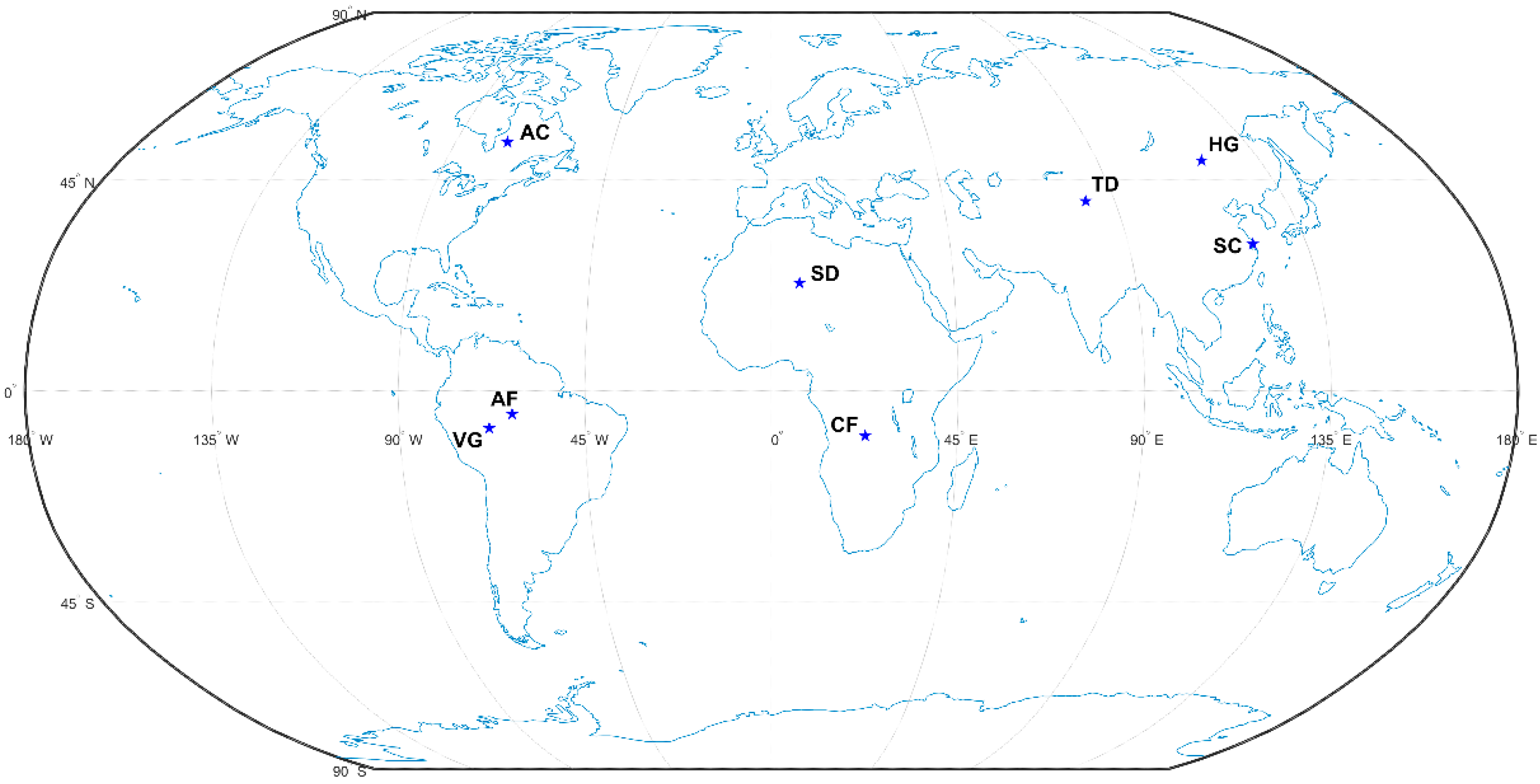
In this study, we select rich experimental data to test the denoising performance of the algorithm. The terrestrial photon-counting LiDAR’s data for four different surface types include woodland, desert, grassland, and urban. In line with [23], the land-cover types are determined by the GLOBELAND30 product in 2020. For every kind of surface, two separate sets of data located at various locations are selected to increase the diversity of the data, and all data (dataset 1~8) are obtained from the ATL03 datasets from the NASA ICESat-2 (version 005) [24]. The geographical locations of eight sites in this study are shown in Figure 1, where the blue asterisk locations are the locations of each study area.
2.1.1. Forest
The study area of the Congo Forest (CF) in Africa has a latitude and longitude range of (9°38′~9°50′N, 22°38′~22°42′E), as shown in the CF map in Figure 2, which has a sizeable topographic relief. And the selected data acquisition time is daytime, so the noise rate is high: about 33.42%. In this paper, we select the 150~153 s data from gt1r in dataset1 as experimental data. The longitude and latitude range of the Amazon Forest (AF) in Brazil is (4°57′~5°12′N, 62°39′~62°33′E), as shown in the AF map in Figure 2. The topographic relief is smaller than the CF, and the noise percentage is only 0.62%. The 78~81 s segment of the gt1l data in dataset2 is selected as the experimental data.
2.1.2. Desert
The study area of the Sahara Desert (SD) in northern Africa has a latitude and longitude range of (22°51′~22°58′N, 6°55′~6°57′E), and the topography of the site is less undulating. We select the data of gt1r in dataset 3 at 63~65 s as the experimental data. The Taklamakan Desert (TD) in Xinjiang, China, has a latitude and longitude range of (40°21′~40°30′N, 82°22′~82°26′E), and the part of gt1r data in dataset4 at 282~284 s is selected as the experimental data. The overall distribution of desert photons is uniform, as seen from Figure 2. And the noise photon rate is low for both desert data due to the acquisition time of night.
2.1.3. Grassland
The longitude and latitude range of the study area of Hulunbuir Grassland (HG) in China is (9°38′~9°50′N, 22°38′~22°42′E). The topography of the site is undulating, and the noise photons account for 62.39%. The 349~351s segment of the gt1r beam of dataset5 is selected as the experimental data. The Venezuelan Grassland (VG) in Venezuela has a latitude and longitude range of (7°58′~8°12′N, 68°14′~68°18′E), and the 125~128 s segment of gt1l in dataset6 is selected as the experimental data. The noise occupation in this region is lower than that of HG, accounting for 17.22%.
2.1.4. City
The longitude and latitude range of the study area in Shanghai, China (SC), is (30°48′~30°56′N, 121°22′~121°26′E), and this area is mostly covered by buildings with a small noise occupation of 5.74%. The 449~451 s segment of gt1l data in dataset7 is selected as the experimental data. The study area of the Atlantic coastal cities of the northeast United States (AC) has a latitude and longitude range of (53°22′~53°30′N, 75°10′~75°18′E). This area’s topography is undulating, and there are no prominent buildings. The noise percentage is about 55.06%, and the 206~208 s segment of gt1l in dataset8 is selected as the experimental data.
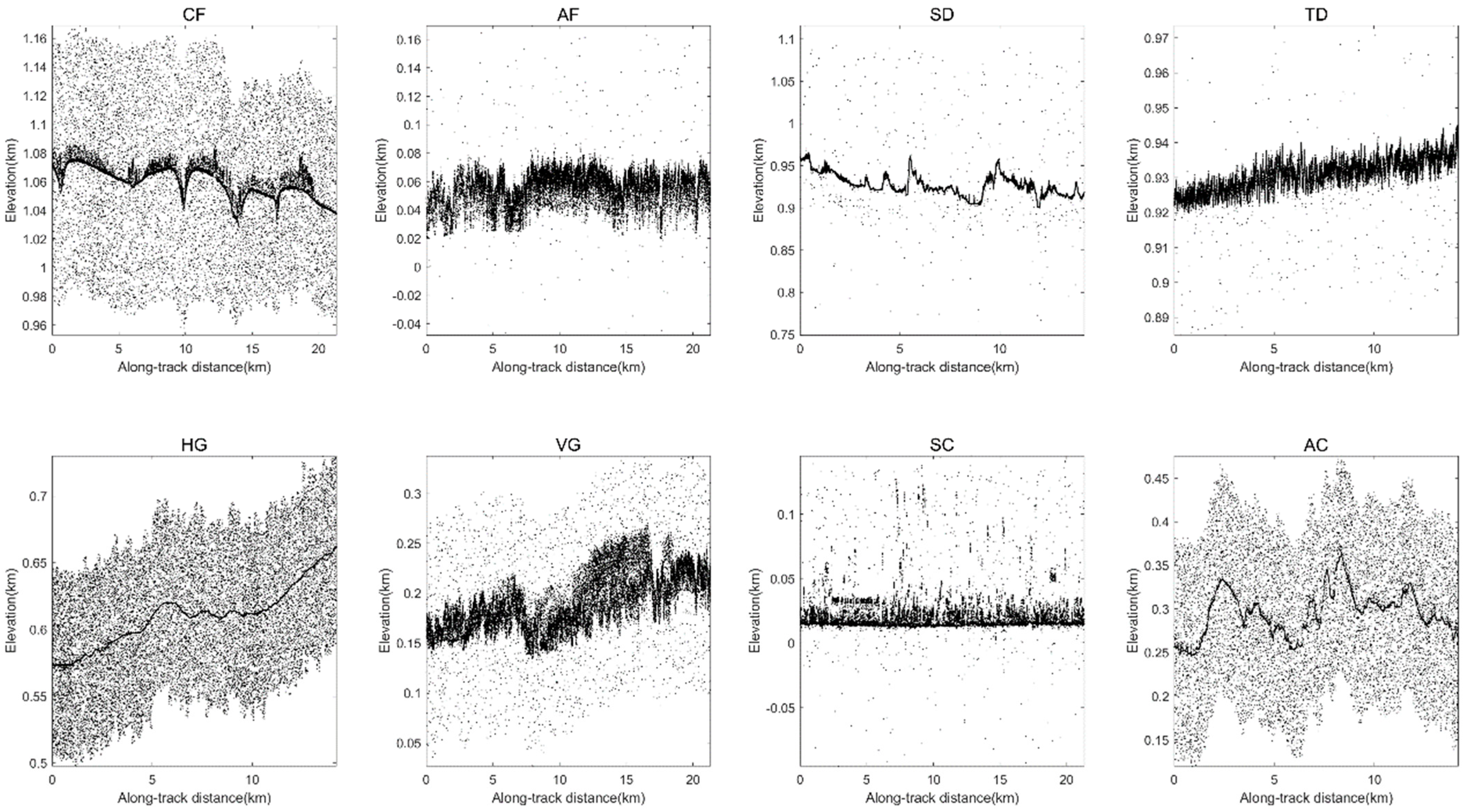
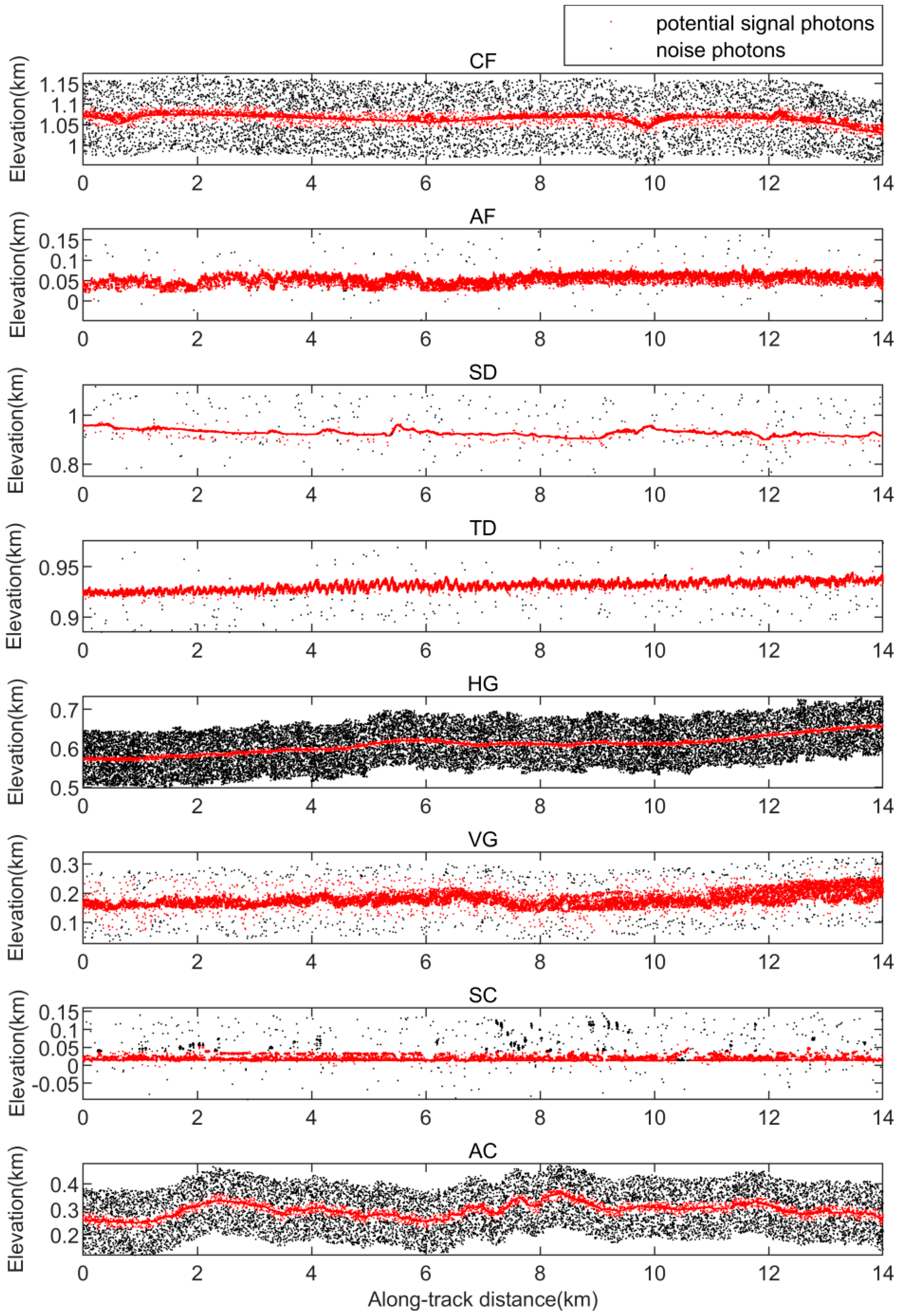
The eight datasets located in different regions of the Earth contain different surface types and topographic variations (woodland, desert, grassland, urban), also include strong and weak beam data, and have different background noise rates (0.62~62.39%). Table 1 summarizes the details of the above data. The photon height distribution of the selected ICESat-2 ATL03 datasets along the track are shown in Figure 2.
2.2. Manually Annotated ICESat-2 Truth Reference Dataset
The ICESat-2 Level-2 ATL03 product classifies each photon into five surface types (land, land ice, sea ice, seawater, and inland water). The measured geolocated photons include signal and noise and are labeled as signal or noise through signal-finding techniques. It provides a preliminary assessment of the confidence level of each photon event (0: noise, 1: added to pad likely signal photon events, 2: low confidence signal, 3: medium confidence signal, 4: high confidence signal) [25].
The ICESat-2 Level-3A ATL08 Land and Vegetation Height data product using the Differential, Regressive and Gaussian Adaptive Nearest Neighbor (DRAGANN) algorithm to denoise the ATL03 data [26], classifying the photon cloud into canopy top photons, canopy photons, ground photons, and noise photons using the official NASA classification algorithm [27]. However, there are still missing signal photons and misclassifications in ATL08 data in some areas with complex topography [23].
Due to insufficient reference data (e.g., airborne LiDAR data) to verify the performance of the proposed method, we interpret the photon type through visual interpretation in this study. Firstly, we refer to the confidence label of ATL03 and the classification label of ATL08 to identify the densest ground signal photons. Then, we search for photons in the range of 0-30 m above the ground photons and compare the elevation data in Google Earth to determine the signal photons [21]. In this study, we use the manually annotated photon data after visual inspection as the actual value for comparing different algorithms.
2.3. Methods
2.3.1. Overview
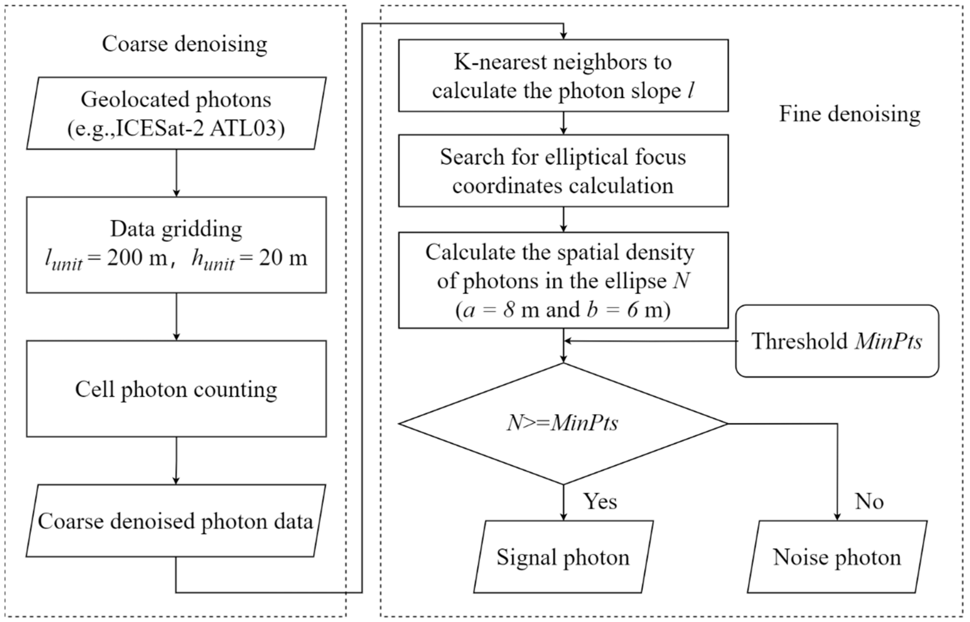
According to the characteristics of uneven distribution of ICESat-2 photon-counting data, we propose a multi-stage adaptive noise-filtering algorithm called MLANF. The algorithm follows a two-step process: coarse denoising and fine denoising. The purpose of the coarse denoising step is mainly to detect the potential signal photon regions. The purpose of the fine denoising step is to optimize the density clustering through the adaptive denoising algorithm. The detailed steps of the MLANF algorithm are shown in Figure 3. The geolocated photons are gridded, and the regions with potentially more signal photons are selected according to the grid density. Then, the circular search area is modified to be elliptical. The direction of the central axis of the search area is automatically changed along the terrain’s slope so that the density clustering results are more closely matched to the signal photon data area.
2.3.2. Coarse Denoising
The raw geolocated photons data can be regarded as 2-dimensional data with an along-track distance in the x-axis direction and elevation in the y-axis direction. By observing the geolocated photons of ATL03 products datasets (Figure 2), the signal photons are uniformly distributed in the x-axis direction and concentrated in the y-axis direction at the middle height position in the overall photon data. Most of these signal photons are soil or vegetation surfaces with high density. In contrast, the noise photons are uniformly distributed along the upper and lower sides of the signal photon. In general, the space occupied by noise photons is larger than that occupied by signal photons, but the density is lower than that of signal photons. According to the above signal and noise photon characteristics, we use a gridding process for the raw photons, e.g., column by column and row by row [18]. Then, the potential signal photon regions are detected according to the number of grid photon points. The specific steps are as follows:
(1) Data gridding
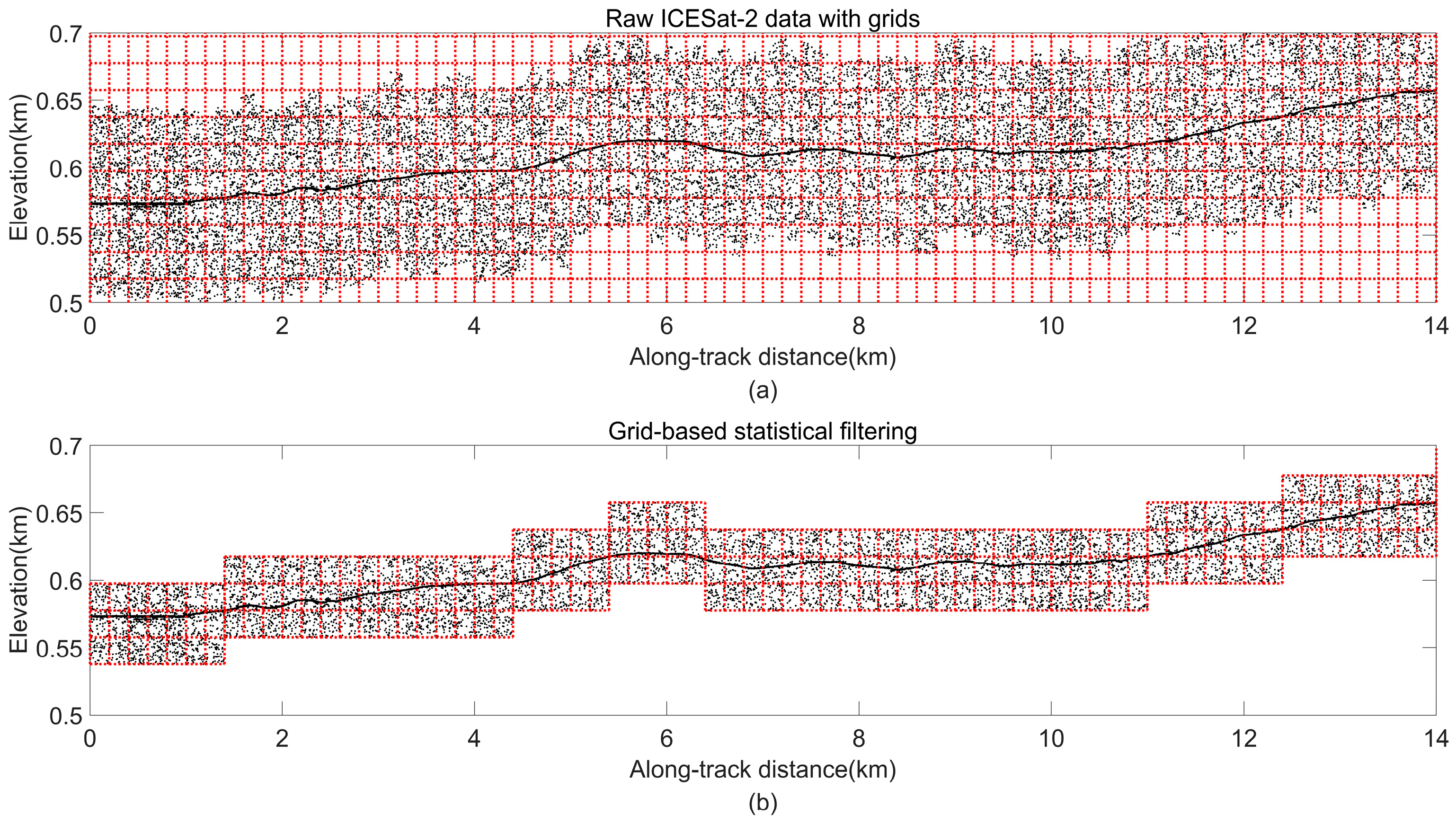
We can easily obtain the track length L and height H of the raw geolocated photons. Then, we construct a grid for the photon data with grid cells whose size is lunit × hunit. The parameter lunit determines the fineness of coarse denoising, and the parameter hunit determines the size of the potential photons region. All photons will be divided into grid cells to realize the data gridding of geolocated photons, as shown in Figure 4a. The size of the grid cell can be decided in two ways. One is set as a fixed percentage, and the grid cell size adaptively changes with the data:
The other way is set as a fixed size. By many experimental tests, we find that the size of the grid cell can be set as 200 m × 20 m. It is suitable for all experimental data.
(2) Cell photons counting
In this step, we count all the grid cell photons, and the number of photons is N(i, j) in each grid cell. Then, we select each grid cell with the highest number of points in the column of grids along the track direction as key cells. To prevent the height change from being too large, we also retain the two grid cells N(i, j + 1) and N(i, j − 1) together as the potential signal photon region, as shown in Figure 4b. To avoid ambiguous situations, the second highest number of photons and their adjacent grid cells are also calculated and compared with the key cells and their neighbors. Finally, we choose to reserve the three grid intervals with the largest sum of photon counts to avoid misidentified signal intervals caused by the close proximity of photon numbers.
2.3.3. Fine Denoising
As shown in Figure 4b, we find that some noise photons still exist above and below the signal photons. In order to extract the signal photons near the surface, we finely denoise the photons through the slope-based adaptive denoising algorithm.
(1) Brief introduction of DBSCAN algorithm
DBSCAN is a classical density-based clustering algorithm [28]. The clustering principle is as follows: a seed point is first randomly selected from the dataset, and the number of points N in the circular search area of a given radius e is calculated. If it is larger than the set MinPts, the point is considered a core point; if not, it is considered a noisy point marked as visited. Then, the process is repeated for the points within the radius of the core point. If a point is a core point, it can be added to the cluster and become part of a class. The process is repeated until all points are visited and marked as different classes with noisy points.
(2) Elliptical search model
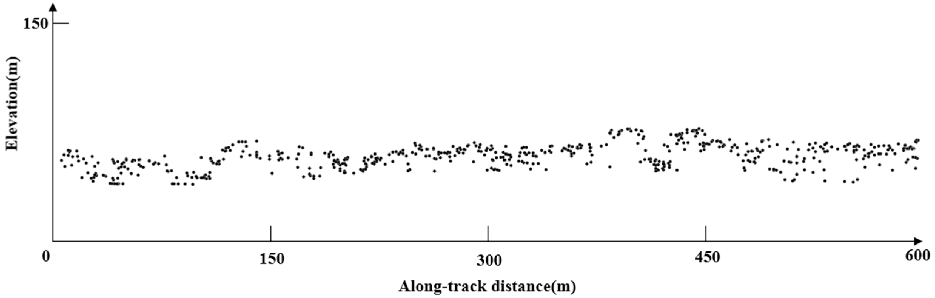
In this paper, we find that the spatial density distribution of the potential signal photons is not uniform. The number of points on the horizontal direction is much larger than the vertical direction, as shown in Figure 5. This unbalanced distribution makes it difficult to use DBSCAN directly because its search model is a circle. We modify the circular search area to an elliptical model based on the DBSCAN algorithm, which can solve the problem of unbalanced point density distribution.
When the horizontal ellipse model is used instead of the circular search region, the key parameters of the horizontal ellipse model are changed from the radius e to the long semi-axis a and the short semi-axis b. In this paper, we still use the Euclidean distance to determine whether a point q is located in the elliptical search region with the core point p as the center. If the distance from the point q to the two focal points c1 and c2 of the ellipse is less than the length of the long axis of the ellipse 2a, the point q is in the search ellipse of the point p, as shown in Figure 6. The distance d from point q to the two foci of the ellipse with core point p as the center is calculated by Equation (3):
where the coordinates of c1 and c2 are calculated by the following:
(3) Adaptive slope search
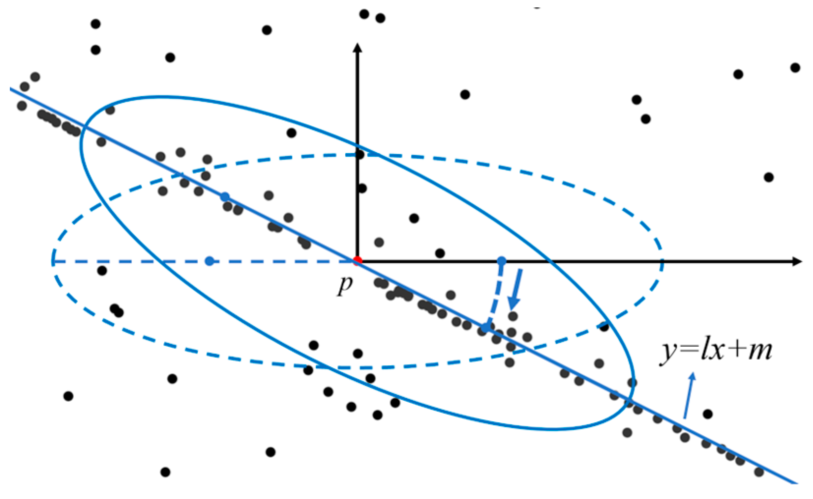
Since the ground surface is not always horizontal and the signal photons are distributed according to the surface shape, it is not flexible to use only the horizontal ellipse model. In order to identify more signal photons, we improve the search model so that its search direction can be changed adaptively. Instead of using the horizontal ellipse search model, we use the slope direction of each photon as the main axis direction of the ellipse search model, which makes the search model more consistent with the direction of the surface and obtains a better clustering effect, as shown in Figure 7.
We consider that the core point and the points in the nearby area have a common slope direction. Based on this assumption, we select k points around the core point by the KNN algorithm. We empirically set k to 50 in all our experiments. And then we utilize the least squares method to fit a straight line along the surface to these points. The objective function of the straight line is as follows:
where l and m are the slope and intercept of the fitted linear, respectively. We consider the direction of the slope of the line as the direction of the long axis of the ellipse model. If the line equation of the surface photons after the least squares fitting is , the two focal points c1 and c2 of the ellipse will be as shown in Equations (7) and (8):
Then, the new distance d of the changed focal coordinates is recalculated according to Equation (3) and compared with the long axis of the ellipse 2a. If d is less than 2a, it means that the point q is in the search range, and if d is greater than 2a, it means that the point q is outside the search range. The number N of photon points in the ellipse can be counted by this changed search method.
In addition, we not only change the search model but also calculate the threshold MinPts adaptively. The number of photon points N in the search ellipse of point p is marked as a visited signal point if it is larger than MinPts. Otherwise, it is a noise point. In this paper, we consider that the size setting of MinPts is related to the average point density ρ of the current data. The higher the density of the data, the larger the value of MinPts. The average point density ρ of the raw photon data is defined as follows:
where is the total number of photons after coarse denoising, and is the grid area after coarse denoising, which is defined as:
where and represent the range of the grid in terms of distance and elevation variation along the track, respectively.
The standard number of points should be calculated from the average point density ρ, defined as:
where is the area of the elliptical search region, which is defined as:
The point density of signal photons should be appropriately higher than the average density of the whole data, so the minimum point threshold MinPts is defined as follows:
where is a constant greater than 1 and is empirically set to 4. The core points are marked as signal photons when the number of photon points N in the search ellipse is greater than MinPts, i.e., greater than times the average number of available points in the ellipse. After traversing each photon, the photons in clusters are all considered as signal photons, and others are considered as noise photons.
2.4. Evaluation Indicators
In this study, to quantitatively evaluate the algorithm denoising effect, we calculate three common accuracy evaluation metrics: Precision, Recall, and F-score [29]. Precision indicates the ratio of the number of photons correctly classified as signals to the number of all detected signal photons. Recall indicates the ratio of the number of photons correctly classified as signals to the number of all correct signal photons. F-score considers both Precision and Recall as a harmonic mean of them. The three metrics are calculated as follows:
TP, FP, and FN denote true positive, false positive, and false negative, respectively. Specifically, TP is the number of photons correctly classified as the signal, FP is the number of photons incorrectly classified as a signal, and FN is the number of photons incorrectly classified as noise.
3. Results
3.1. Coarse Denoising Results
We use coarse denoising to the raw photon data in eight study regions separately. To better obtain coarse denoising results, we tune the grid size to each region based on the size of 200 m × 20 m. Figure 8 shows the results of eight study areas. The red dot set represents the signal photons after coarse denoising, and the black dot set represents the filtered noise photons.
3.2. Overall Denoising Result
After coarse denoising, we perform fine denoising on eight datasets and show the final results of the photon data by the MLANF algorithm. In the qualitative results of each study area, we add the trajectories of image data from Google Earth with the corresponding photon data to enhance the visualization effect. We also add the truth value by the visual inspection and photon denoising results of three different algorithms to obtain a better qualitative result comparison.
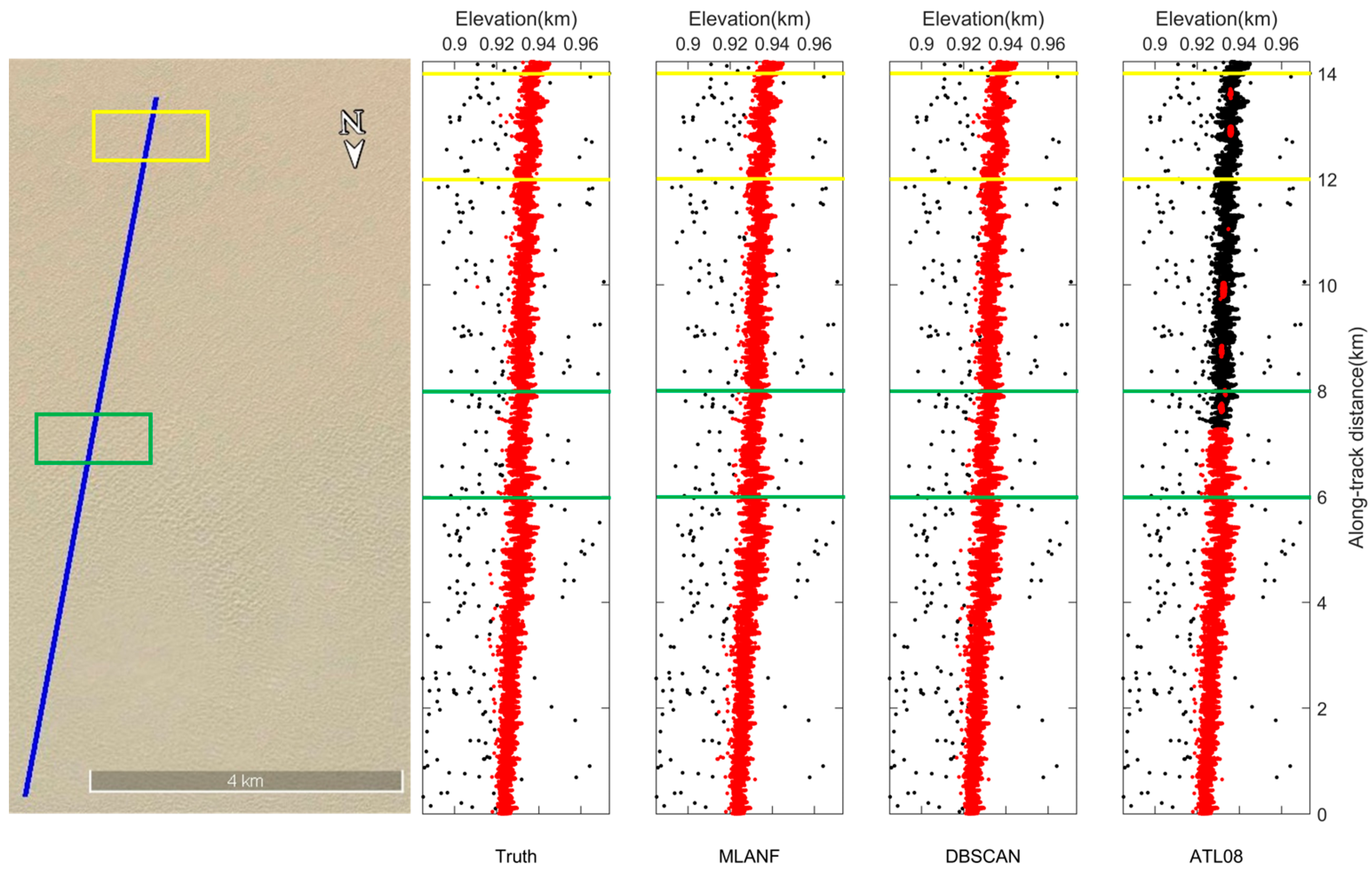
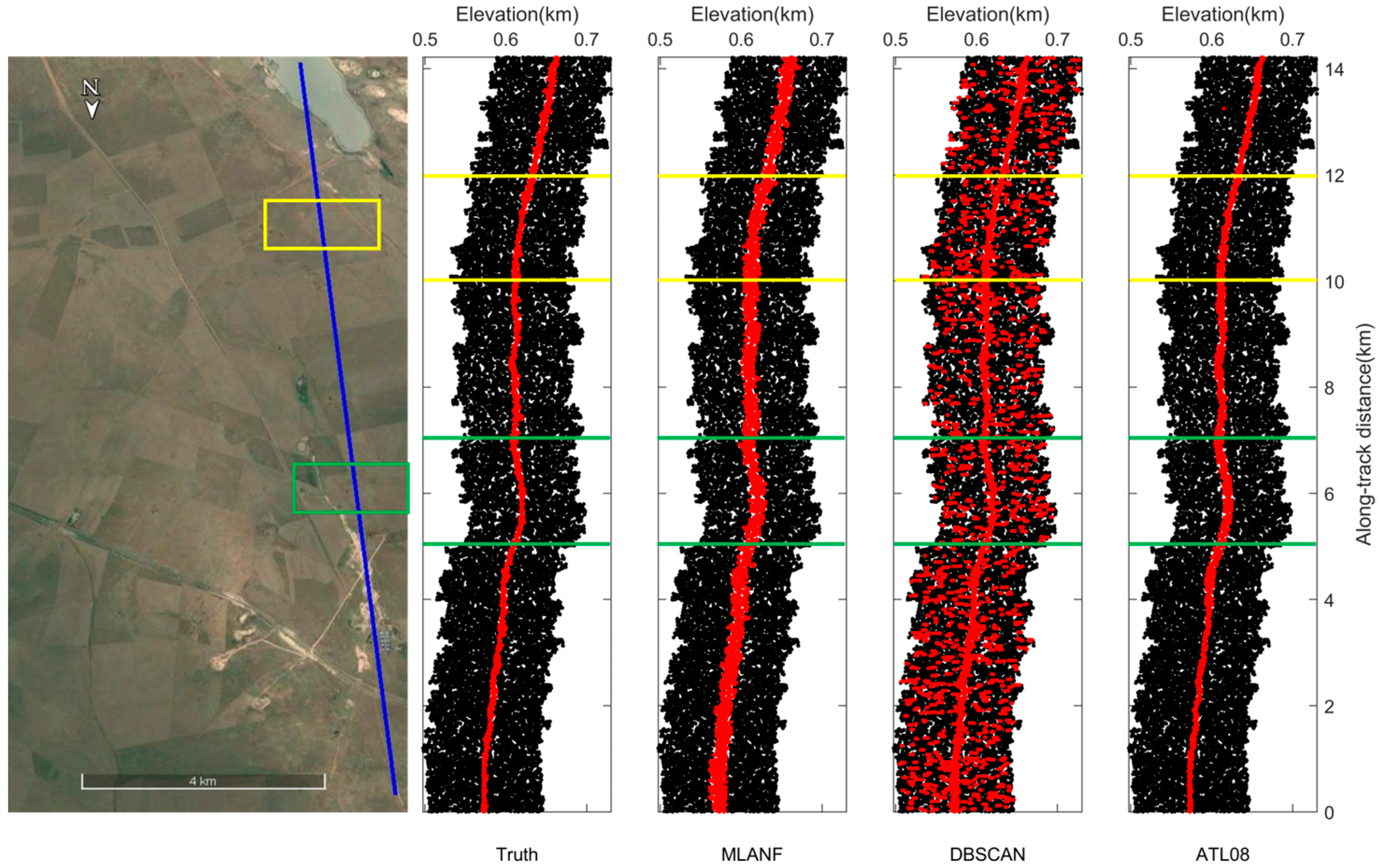
Macroscopically, we show the overall qualitative denoising results of the three algorithms. Each column from left to right corresponds to the signal and noise photons extracted from the manually labeled ATL03 truth dataset, the denoised classification results of the MLANF algorithm, the denoised classification results of the DBSCAN algorithm, and the labeled signal and noise photons from the ATL08 product. Microscopically, two selected regions in each data are zoomed in to show the differences in details of the denoising effects of different methods. Each row from top to bottom corresponds to the signal photon extraction results of the ATL03 manually labeled truth dataset, MLANF algorithm, DBSCAN algorithm, and ATL08 dataset, respectively. In the qualitative results of photon denoising, noise photons are plotted with black dots and signal photons are marked with red dots.
3.2.1. Forest
In the surface data types of forests, we use MLANF for the Congo Forest (CF) and the Amazon Forest (AF), respectively. The photons densities of the two datasets of forests are different. The Congo Forest is a strong beam data with a lot of noise photons, and the Amazon Forest is a weak beam data with a lower number of noise photons.
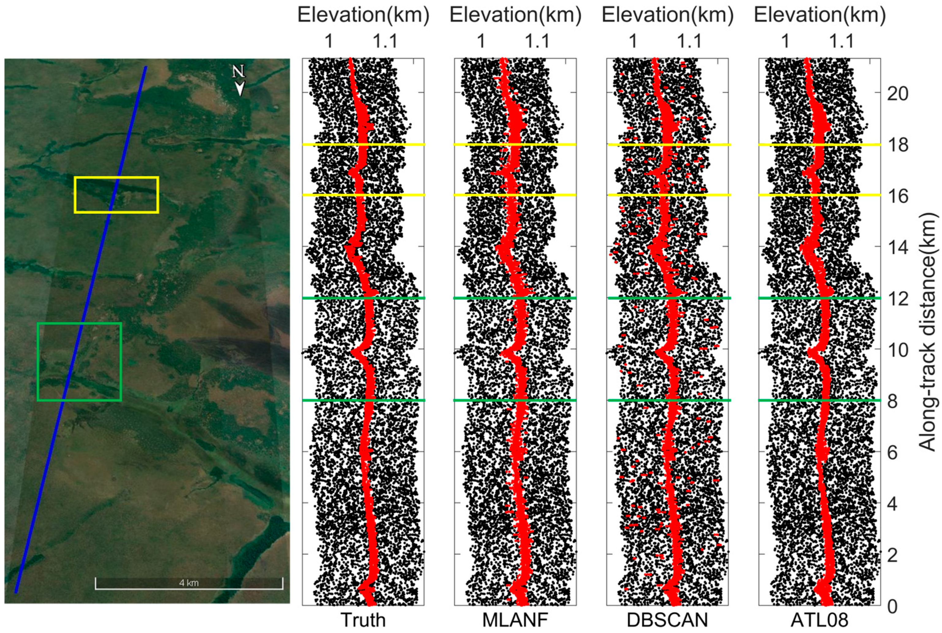
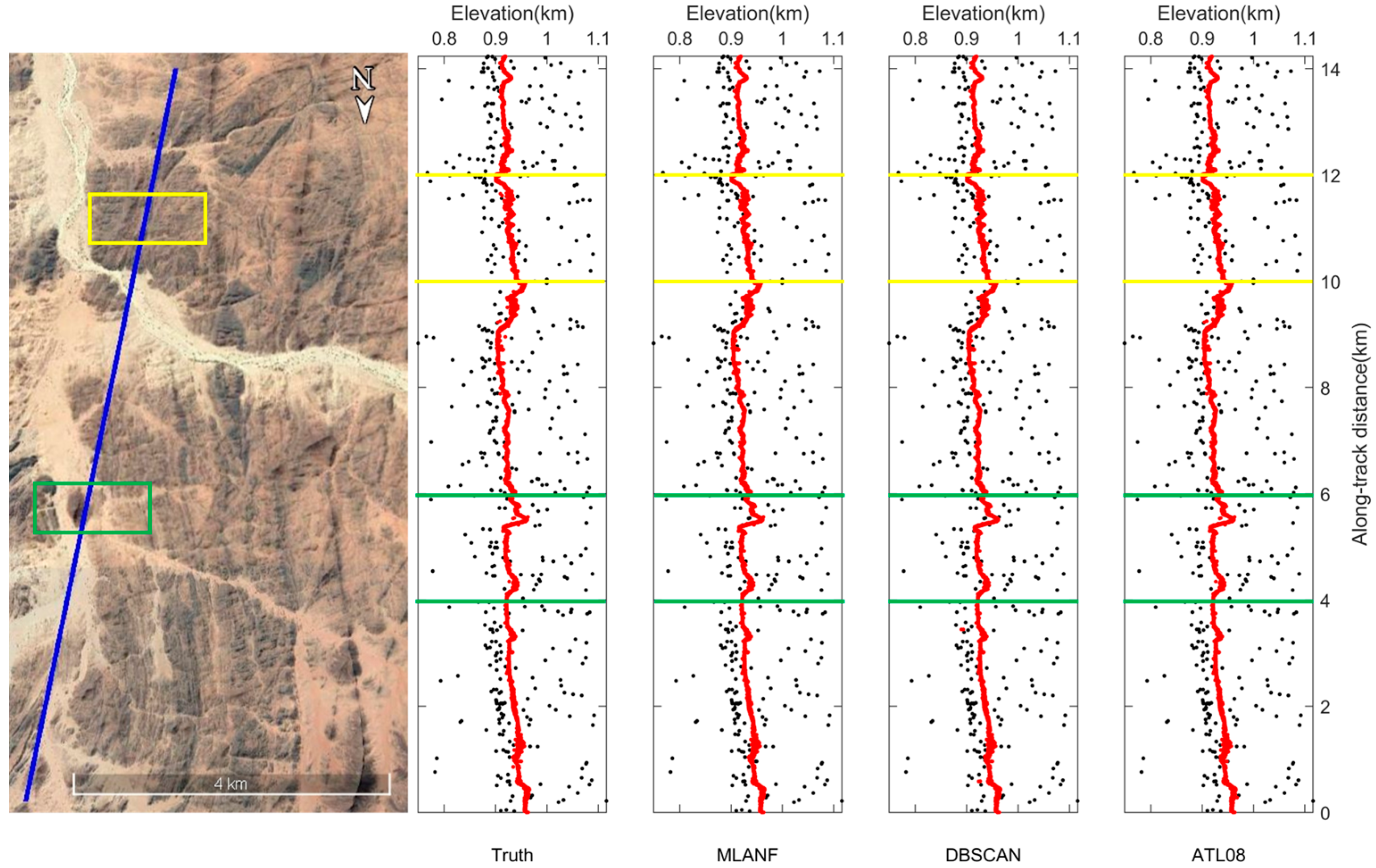
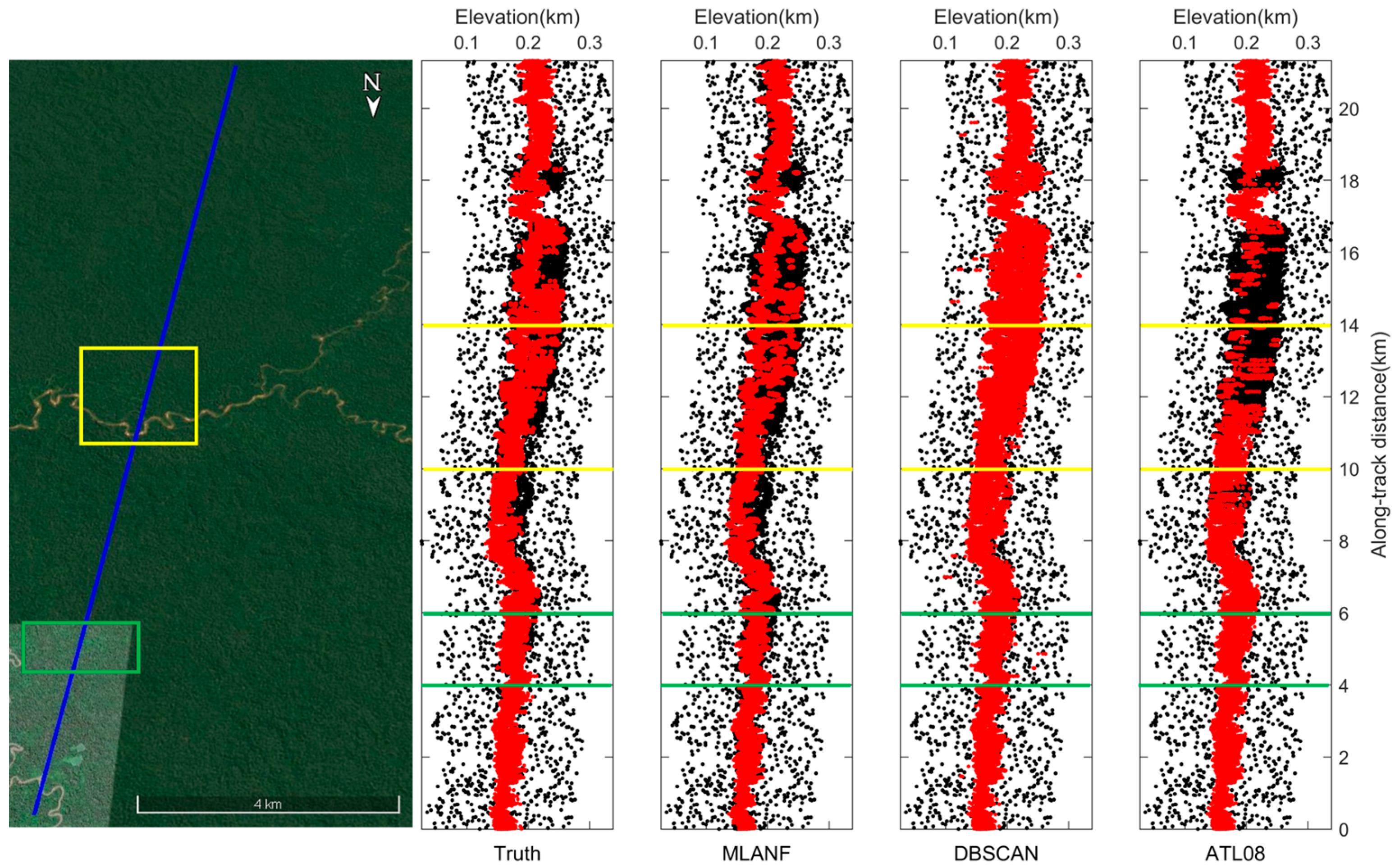
The overall denoising results of the raw photons of the Congo Forest are shown in Figure 9, where the corresponding Google Earth image with the photon track (the straight blue line in the image in Figure 9) is shown on the left. From the image data and the visually interpreted photon distribution, there is an undulating variation in the ground surface covering the grassland and forest vegetation in this approximately 20 km track. On the right side is the actual photon signal distribution of the visual inspection and the denoising results of the three methods.
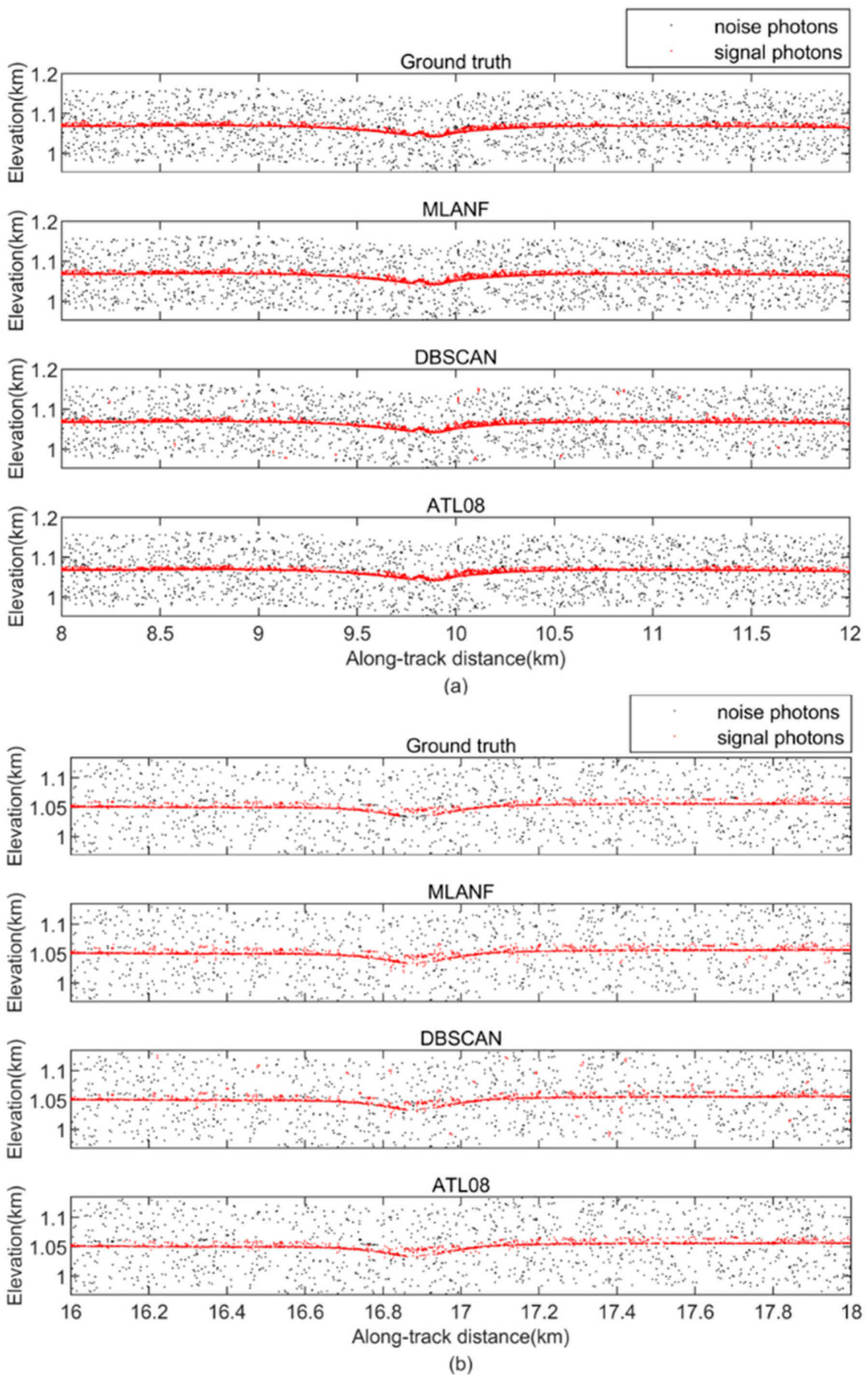
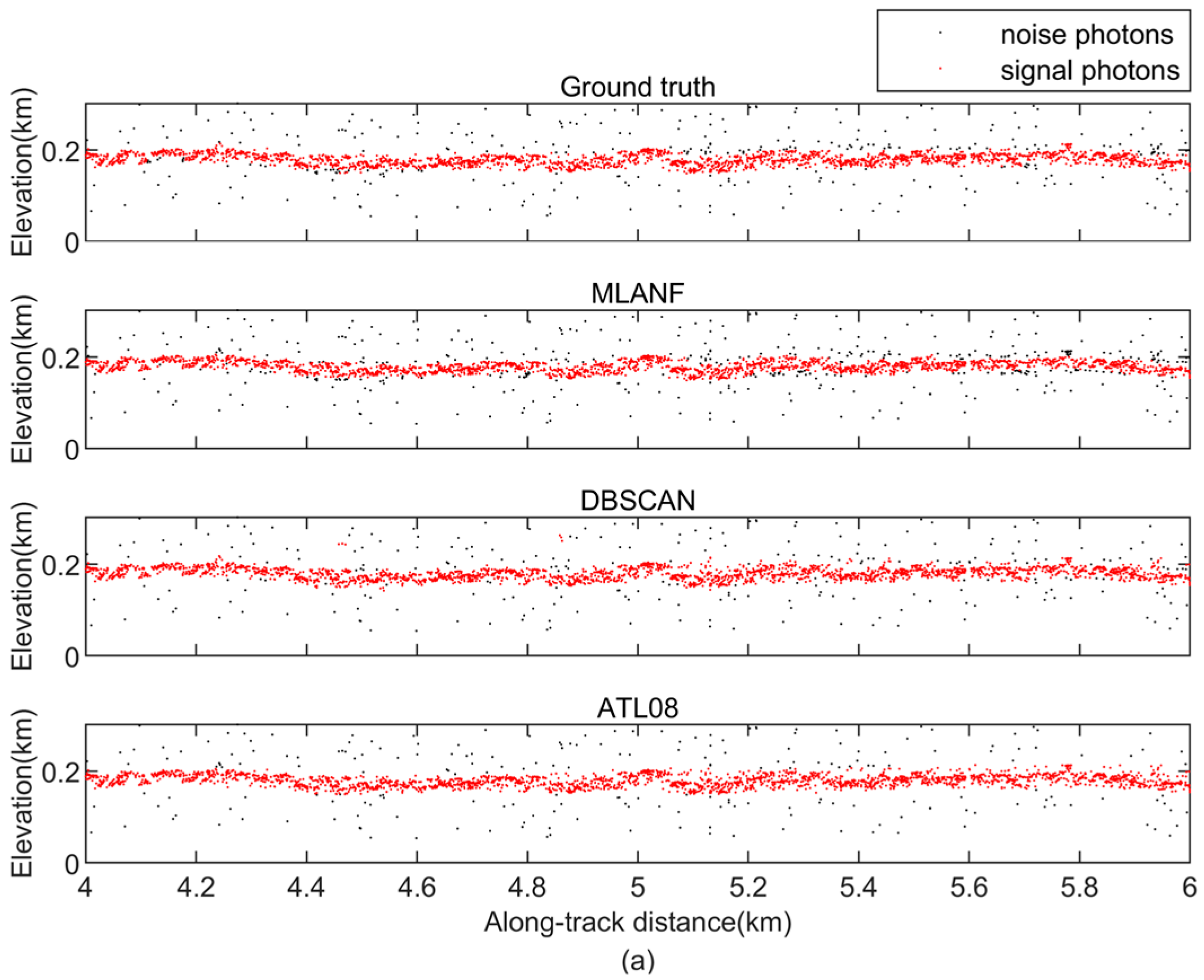
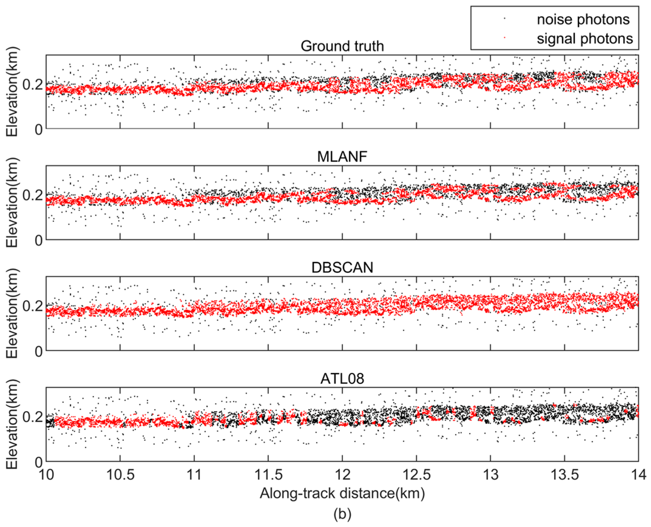
In this region, there is a large amount of random noise on both sides of the surface. We find that all three methods achieve good denoising results. These methods distinguish the ground surface from the random noise and retain most of the signal photons. But the result of the DBSCAN algorithm is weaker than the results of ATL08, and the results of ATL08 are closer to the truth data obtained from visual inspection. Our algorithm is also close to the truth data and the results of the ATL08 product data. Figure 10 shows the detailed results of 8~12 km (green interval) and 16~18 km (yellow interval) in this region.
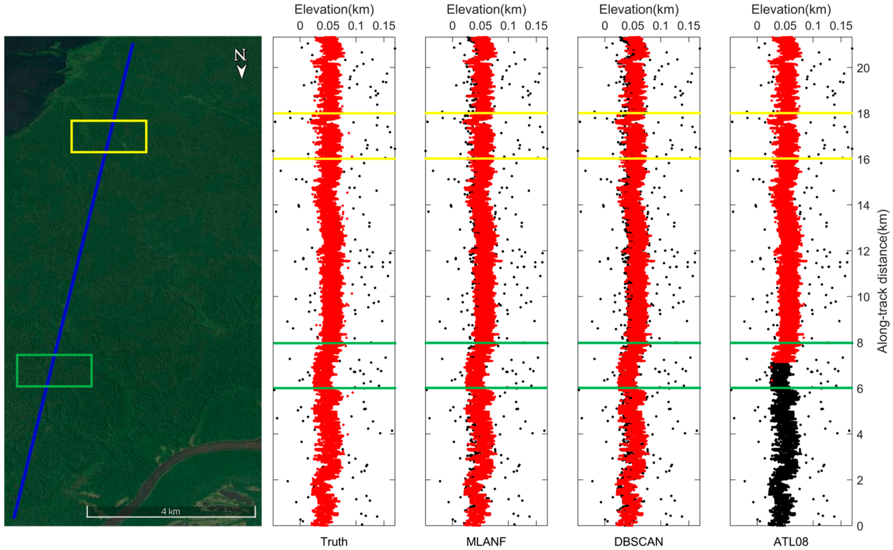
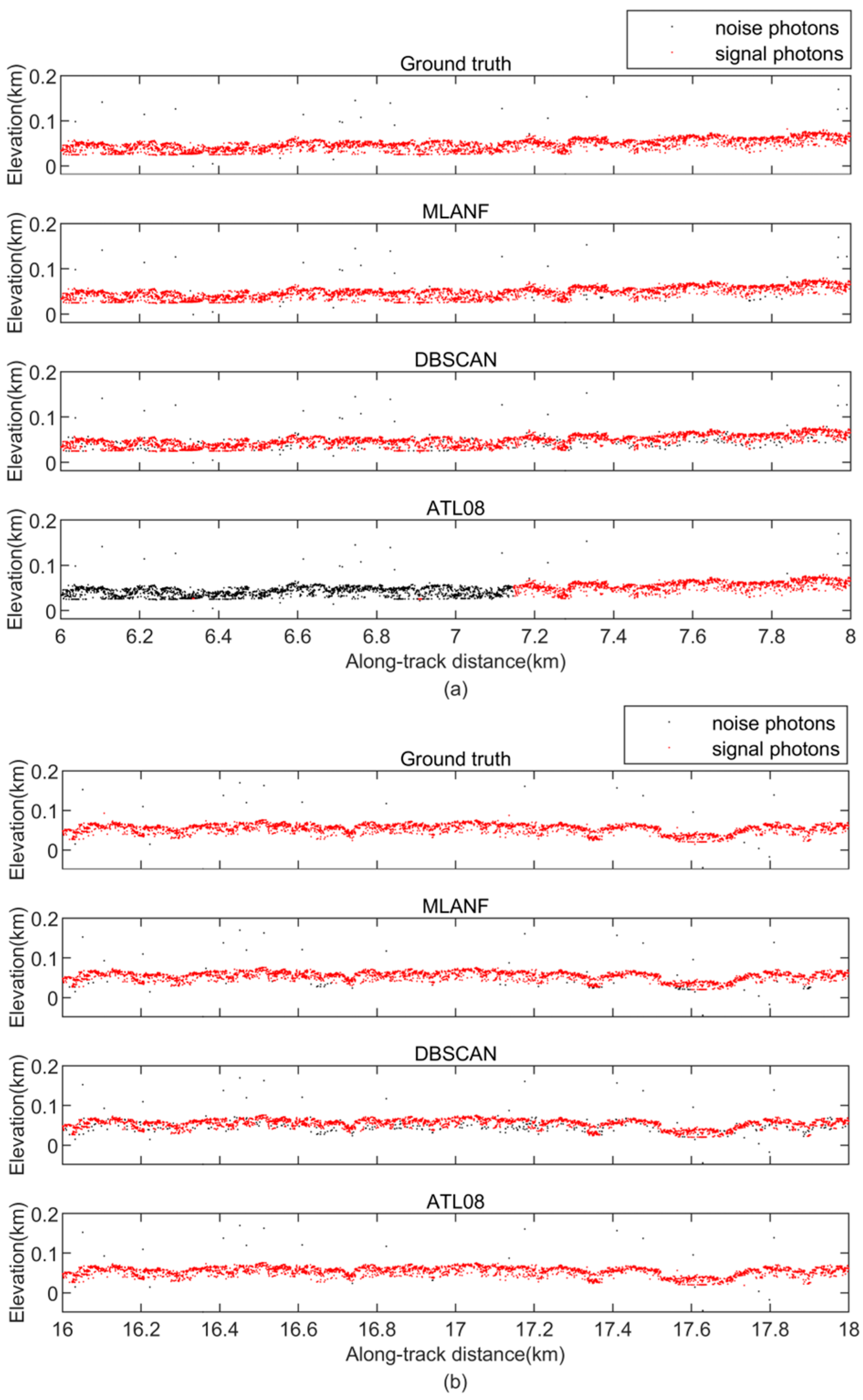
The denoising results of the geolocated photons of the Amazon Forest are shown in Figure 11. The overall track length of this section is about 20 km, and the elevation variation range is more noticeable than that of the Congo Forest. We find that the area is mainly covered with tall forest vegetation. As these photon data are from the gt1r track, the overall photon data have less random noise. The MLANF algorithm and the DBSCAN algorithm have better denoising effects. The ATL08 data have some missing signal data at 0~7 km, and the signal photon extraction result in the latter half is close to the truth value. Figure 12 shows the detailed results of 6~8 km (green interval) and 16~18 km (yellow interval) in this region. At 6~8 km, the result of our method is closer to the truth value than the other two algorithms. The DBSCAN algorithm misclassifies some signal photons as noise photons, and the result of ATL08 misses some signal photon data. At 16~18 km, the result of ATL08 is more similar to the truth. MLANF and the DBSCAN algorithm have a few signal photon extraction errors.
3.2.2. Desert
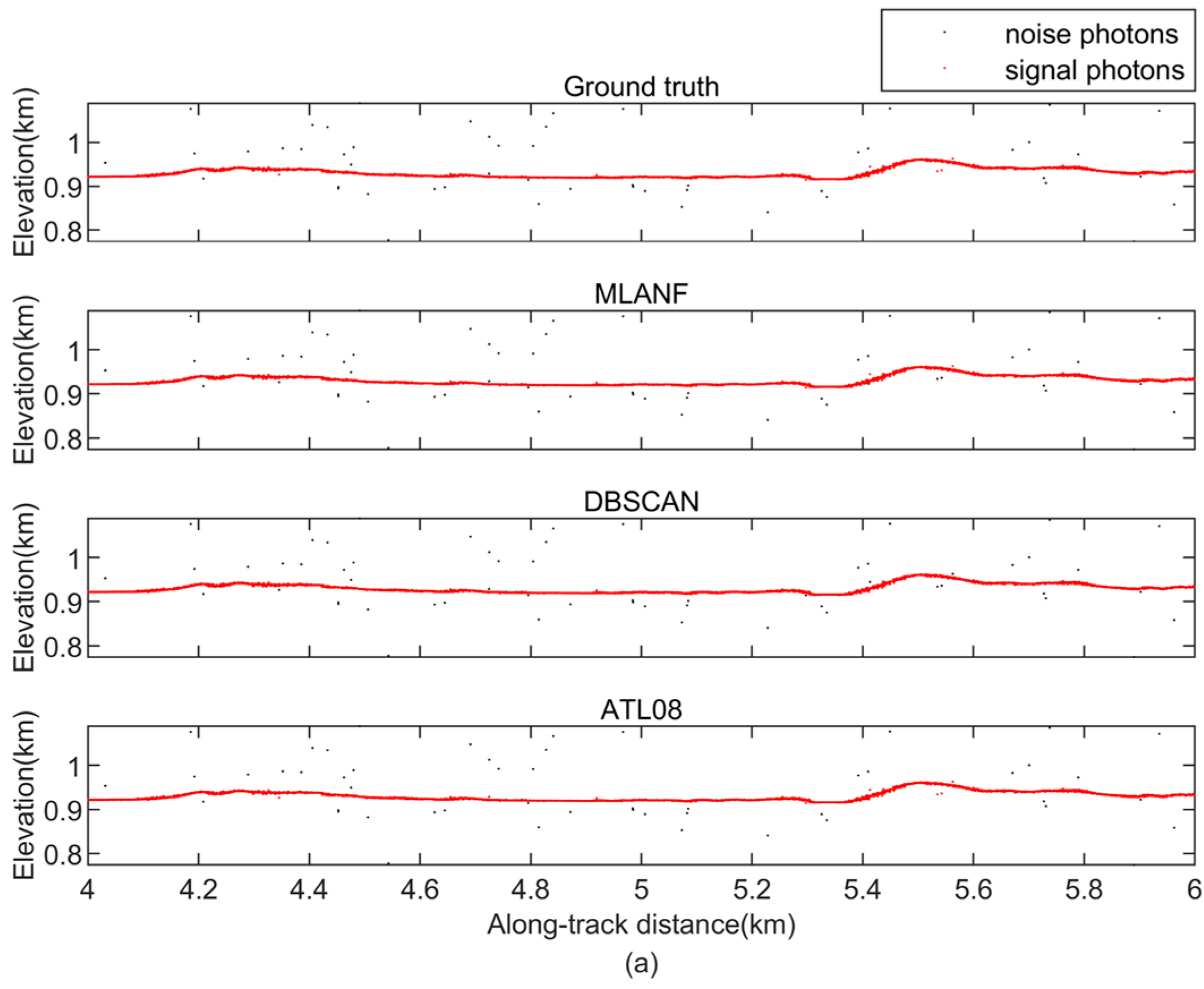
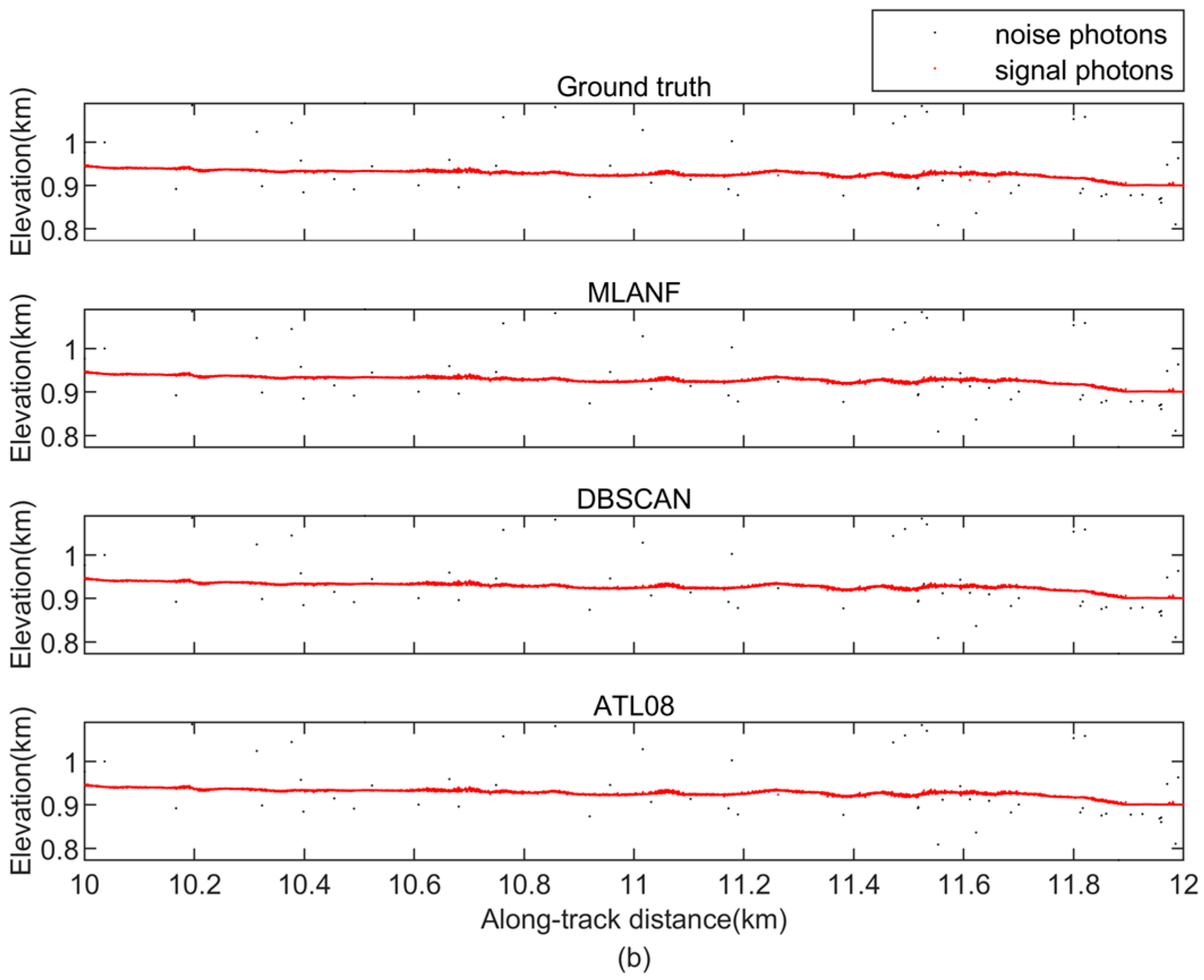
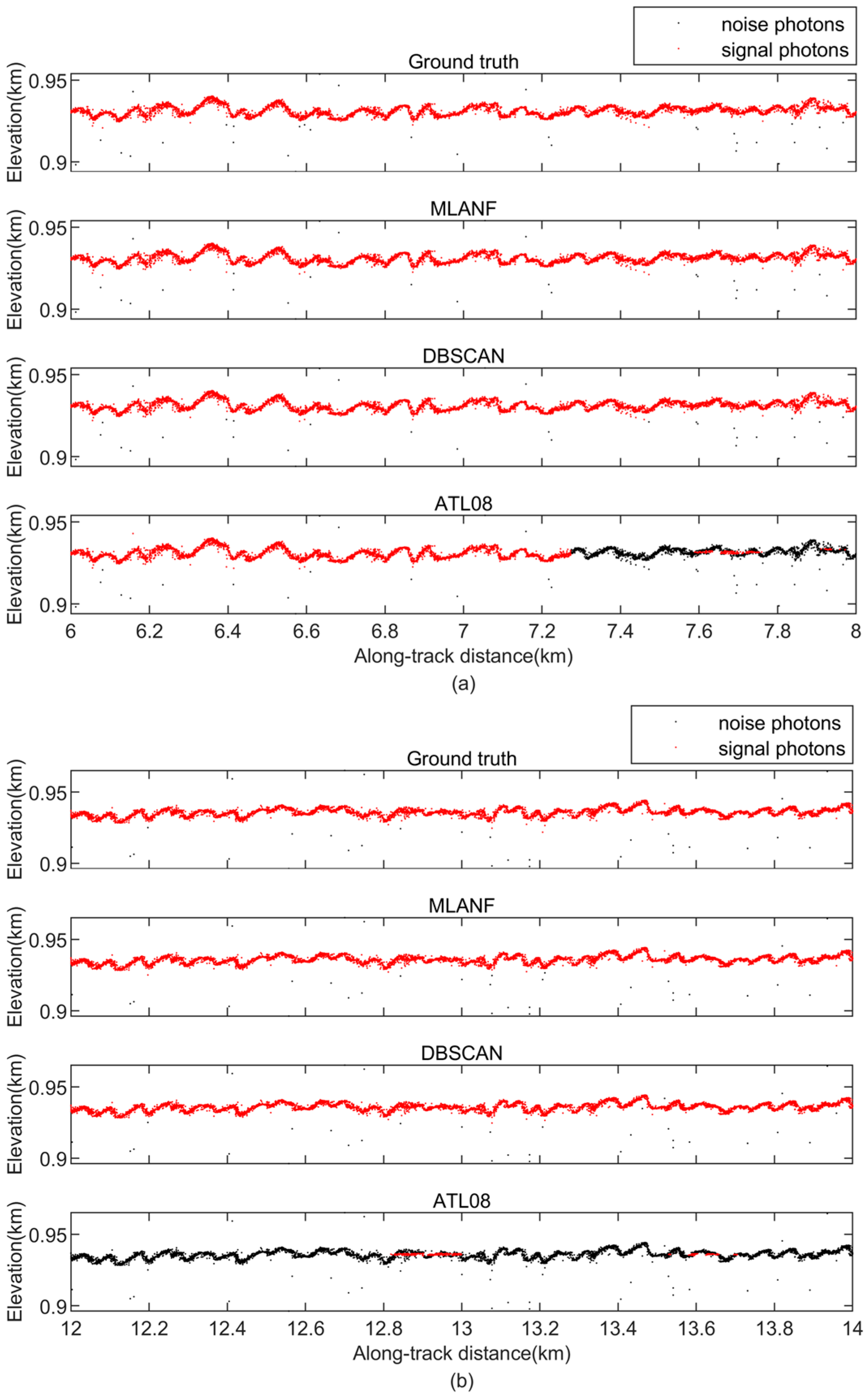
In the surface data types of deserts, we use MLANF for the Sahara Desert (SD) and Taklamakan Desert (TD) data, respectively. The denoising results of the ATL03 dataset in the Sahara Desert region are shown in Figure 13. This region of geolocated photons data is about 14 km with undulating terrain and no vegetation coverage. The proportion of random noise photons is much lower than that of signal photons. So, all three algorithms have good denoising results and extract the desert surface accurately. To further confirm the conclusion, we show the detailed results at 4~6 km (green interval) and 10~12 km (yellow interval) in Figure 14. The signal photons in the desert terrain are distributed in a line shape and are far away from the random noise photons in two intervals. It is easy to distinguish, so three algorithms can easily mark the signal photons with good denoising effect.
Figure 15 shows the denoising results of the TD dataset. This area has many ravines and no vegetation. Like the Sahara Desert data, the signal photons are distributed with less random noise. Three algorithms detect signal photons accurately. The DBSCAN and MLANF algorithms can obtain an excellent denoising effect. But some regions in the ATL08 data are missing signal photons. We show the detailed results of 6~8 km (green interval) and 12~14 km (yellow interval) in Figure 16. The signal photons in this region fit the ground surface and represent the shape of undulating dunes. The signal photons are far away from the noise photons and are easy to distinguish.
3.2.3. Grassland
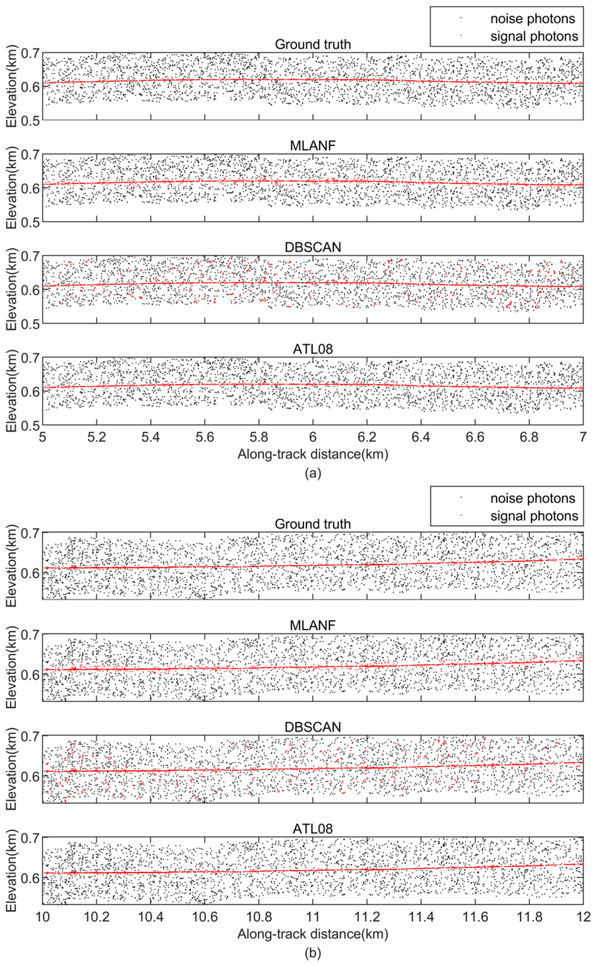
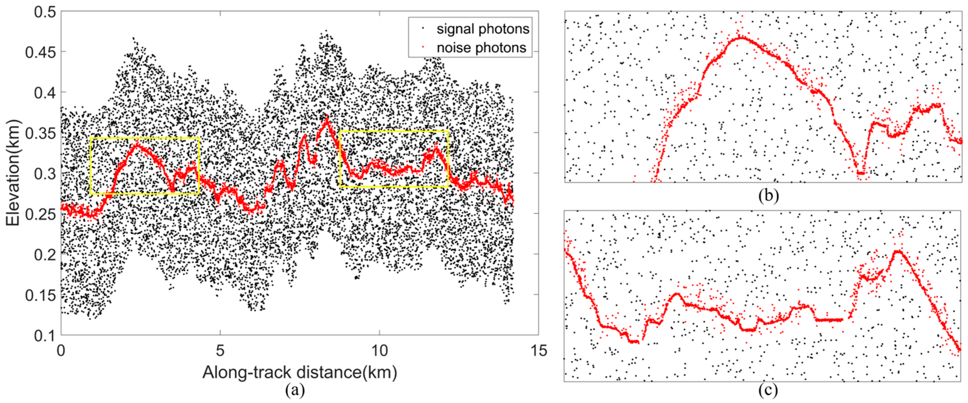
Figure 17 shows the HG dataset’s photon-counting LiDAR denoising results. This segment length is about 14 km. We observe that lots of random noise photons are distributed above and below the signal photons. In the DBSCAN results, the noise photons are marked as signals in the higher-density areas, resulting in some errors. The DBSCAN algorithm cannot filter the noise photons in this region due to its sensitivity to the density. The results of our method and the ATL08 data are closer to the actual surface. The data from the 5–7 km (green interval) and 10–12 km (yellow interval) regions are zoomed in for detailed display, as shown in Figure 18.
Figure 19 shows the denoising results of the photon-counting LiDAR of the VG dataset. This region is located in the grassland of Venezuela, and the segment length of geolocated photons is about 21 km with a large amount of grassland vegetation. The DBSCAN algorithm marks the high-density photon region as signal photons. Our method and the ATL08 data are more accurate and obtain similar results. We show the detailed results at 4~6 km (green interval) and 10~14 km (yellow interval) in Figure 20. In detail, the DBSCAN denoising method successfully identifies the photons in the high-density region, but it is difficult to eliminate the other high-density noisy photon data.
3.2.4. City
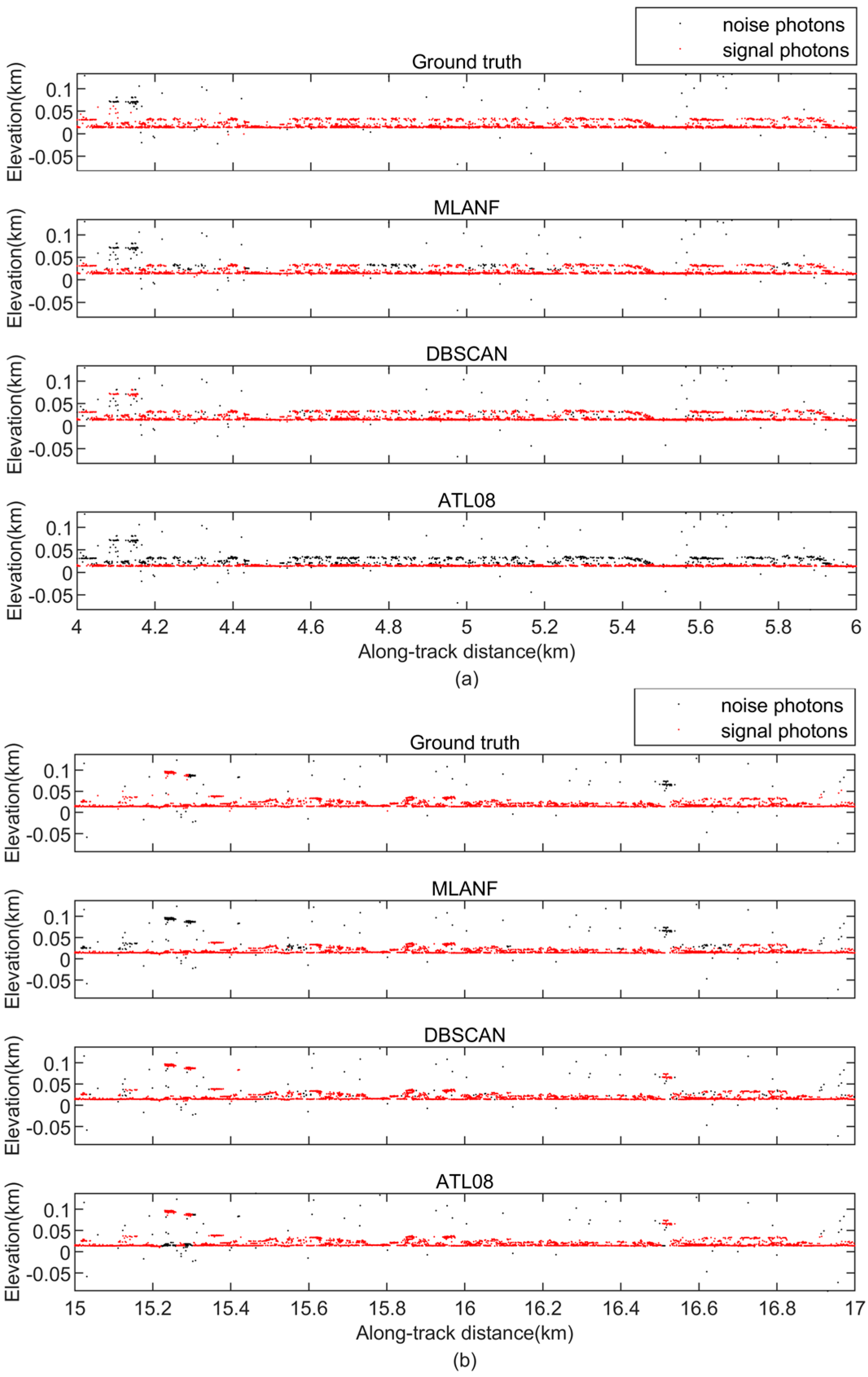
In the urban surface data types, we show the denoising results in two datasets: the Shanghai metropolitan area (SC) and the northeastern Atlantic coastal urban area (HC) of the U.S. The denoising results of the photon-counting LiDAR for the SC dataset are shown in Figure 21. The ground of this region is flat and there are a lot of buildings. A few random noise photons exist below the signal photons and more noise photons exist above. The DBSCAN algorithm identifies the high-density photon data as signals and marks a little noise as signal data. The ATL08 data have a higher error rate in the 0–8 km segment. The denoising result of ours is closer to the true surface. We also show the detailed results at 4~6 km and 15~17 km in Figure 22.
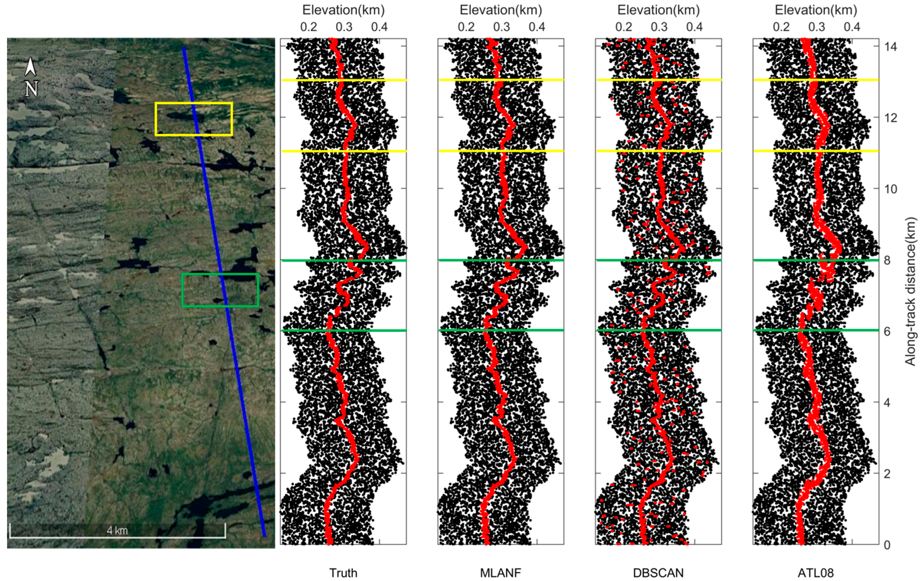
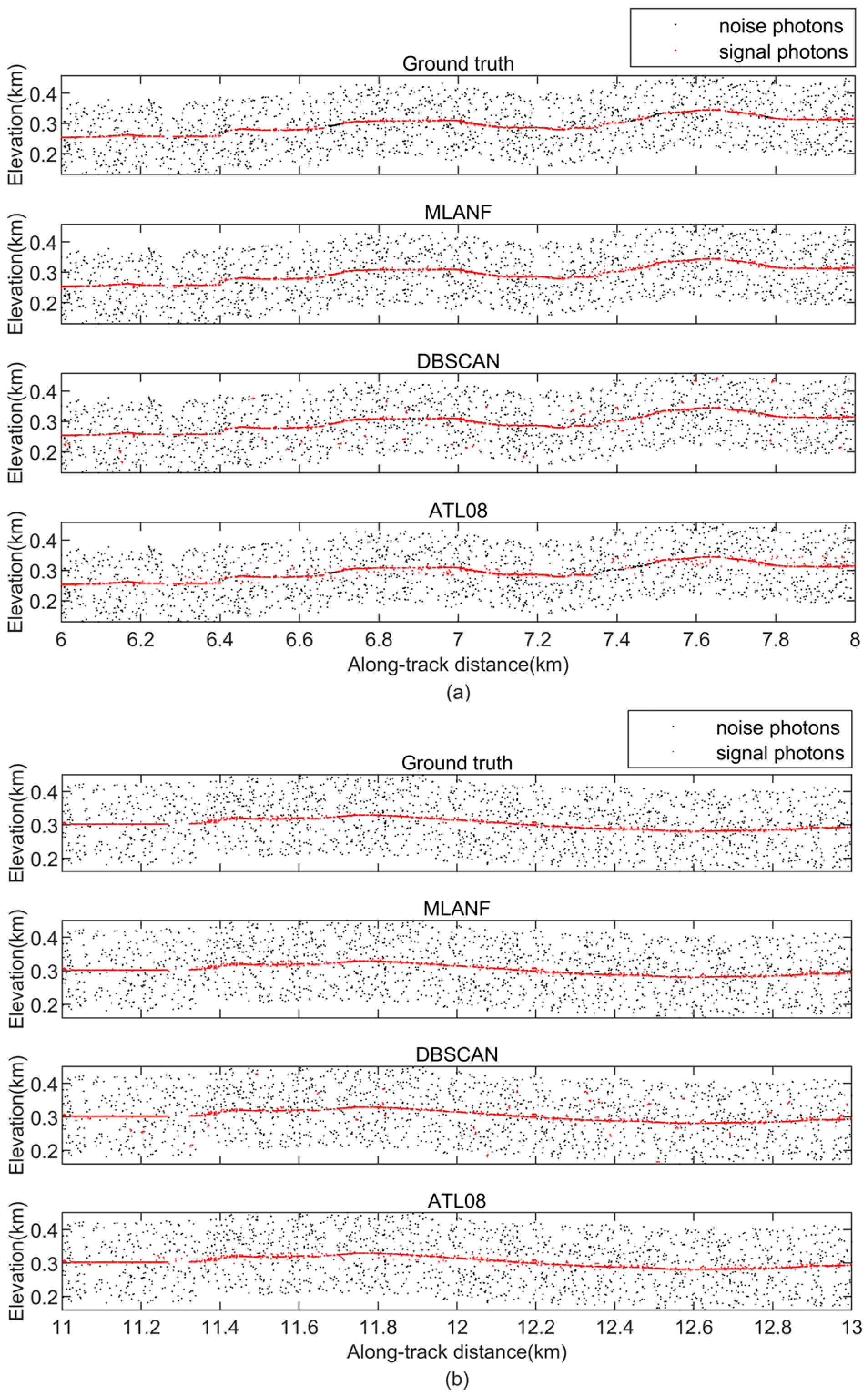
Figure 23 shows the photon-counting LiDAR denoising results of the HC dataset. This segment length is about 14 km with a lot of random noise photons. The area is mainly bare and leaky ground with less vegetation, so the signal photons are fitted to the ground surface. The DBSCAN algorithm is more sensitive to density, so its result has some misclassifications in the region of higher density. Our method and the ATL08 data are more accurate than DBSCAN. Figure 24 shows the detailed results at 6~8 km (green interval) and 11~13 km (yellow interval) in this region.
In summary, through the qualitative analysis of the three algorithms in eight datasets, we find that the denoising results of the DBSCAN algorithm generally misclassify the dense noise as signal due to its high sensitivity of density. The data of ATL08 extract the signal photons using the DRAGANN algorithm based on the ATL03 product, and the classification results are more accurate. But it always suffers from missing data in some regions. The MLANF algorithm first filters a lot of random noise photons by coarse denoising and then modifies the search model based on spatial density clustering. Finally, we added adaptive slope to the photon search ellipse so that the classification effect is more accurate.
4. Discussion
In the discussion section, we separately quantified the two main processes (coarse denoising and fine denoising) of the MLANF algorithm.
4.1. The Discussion of Coarse denoising result
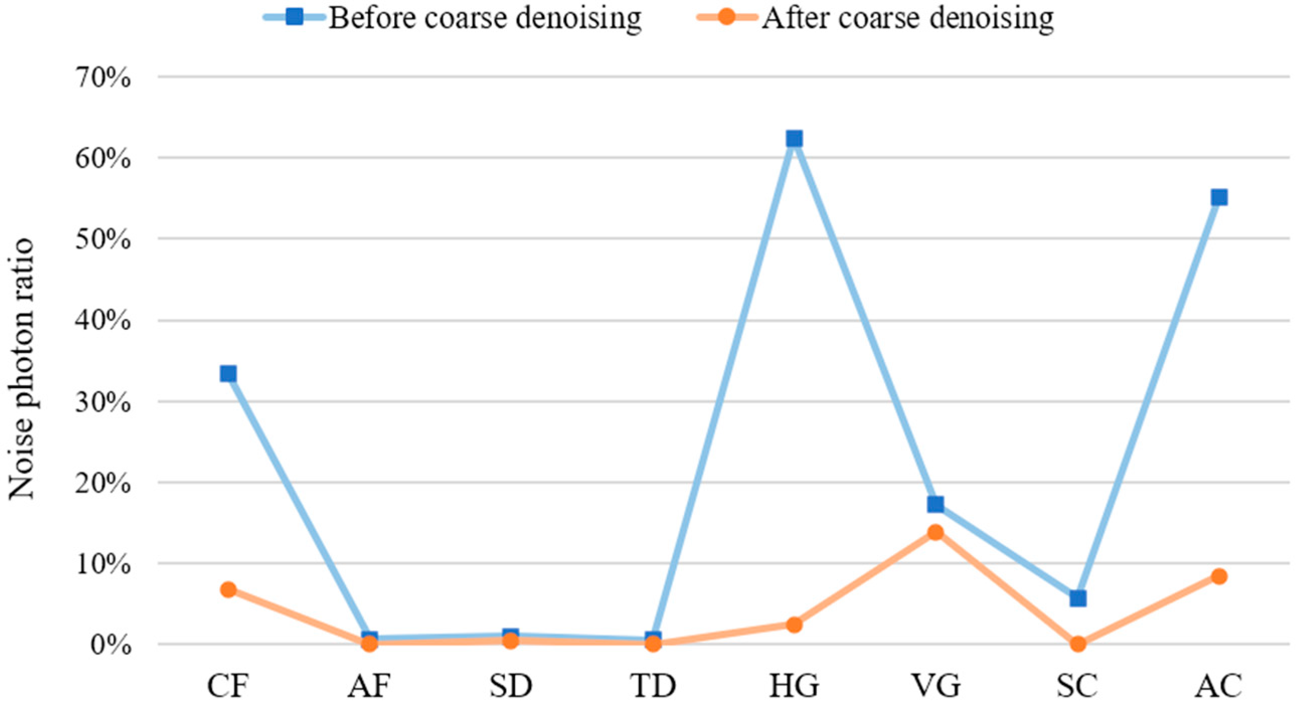
In this part, we calculate the signal photon ratio and noise photon ratio before and after coarse denoising. Table 2 also show the ratio of outlier photons, which denotes the reduction in noise photons. We find that the signal photon ratio only drops slightly in the AF and SC data. This means that the photon data filtered contain almost no signal photons. After the coarse denoising process, the proportion of noise photons is significantly reduced especially in the study area with high background noise. The results indicate that the random noise photons are effectively filtered out by coarse denoising, as shown in Figure 25.
4.2. The Discussion of MLANF Denoising Result
Table 3 shows three accuracy metrics of different methods, Precision, Recall, and F-score. We analyze and discuss the quantitative results of the MLANF algorithm, DBSCAN algorithm, and DRAGANN algorithm of ATL08. For each of the four different types of land experimental areas, we discussed them in detail.
- Forest: Three methods all have a lower precision in CF region. The DBSCAN algorithm misclassifies some noise photons as signal photons in CF. The DRAGANN algorithm of ATL08 fails to identify some signal photons in AF and has a lower recall in the forest region. The MLANF algorithm performs well in terms of precision and recall.
- Desert: The results of three algorithms in SD about three metrics are all greater than 99%. The DRAGANN algorithm of the ATL08 cannot identify the signal photons in the TD region, and the recall of it is only 53.43%. Therefore, the other denoising results of the two density-based methods perform well.
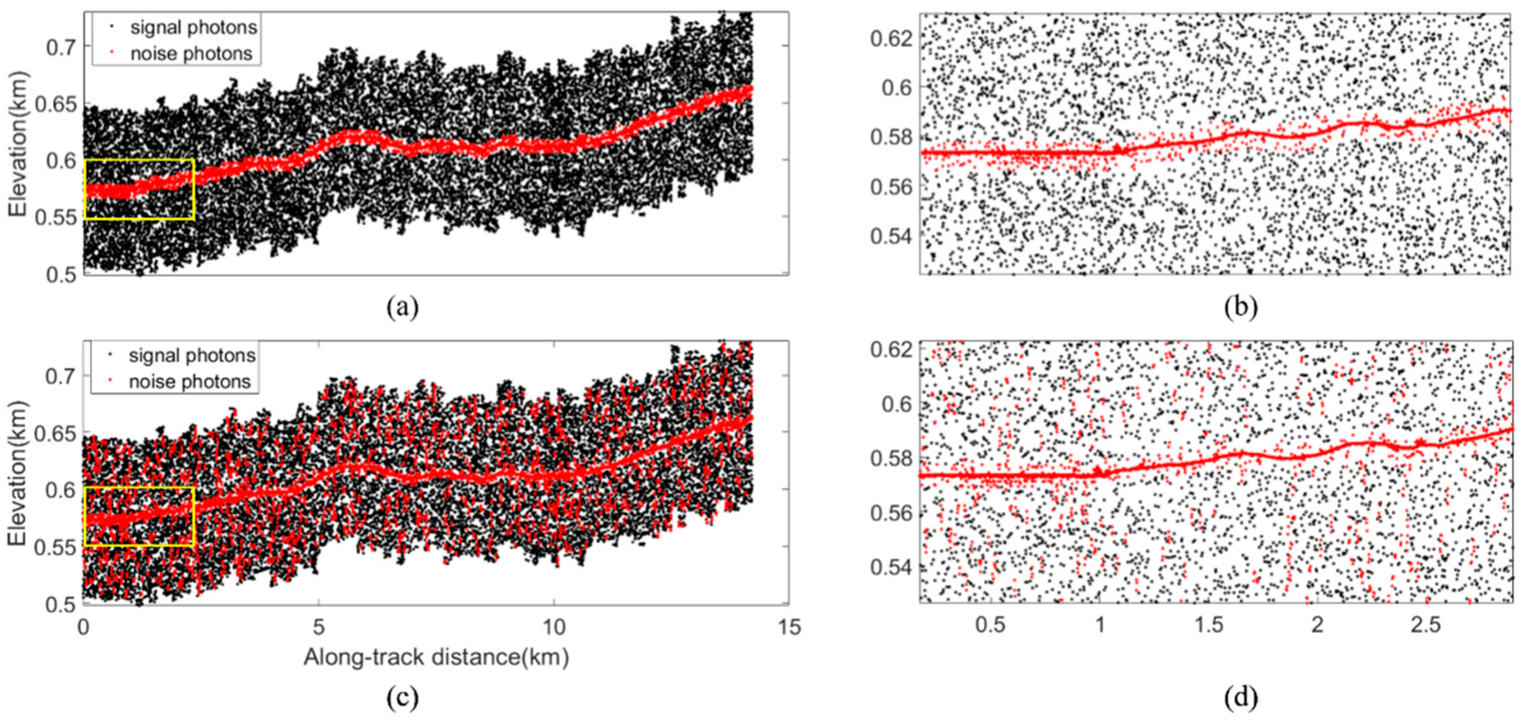
- Grassland: The grassland data all have lots of random noise photons, and their evaluation metrics are lower than those of the other land types. The HG data have a lower SNR than VG data, which seriously affects the accuracy of the three algorithms. As shown in Figure 26, the DBSCAN algorithm results have more errors of misclassification than the MLANF algorithm results. Compared with the other two methods, our method has the best data-denoising effect for the grassland-type data.
- City: In the SC study area, the precision of the MLANF algorithm is 98.22, which is better than that of the other two methods. And the DBSCAN algorithm has a higher recall rate, so its comprehensive evaluation index F-score is better than that of the other methods. Moreover, in the AC study area, the precision and recall value of our algorithm in this paper is high, so the comprehensive evaluation index F-score is the highest. In contrast, the DBSCAN algorithm and ATL08 have lower precision and recall values, so the quantitative evaluation results are lower than those of our method. Figure 27 shows the denoising results of the MLANF algorithm in the AC area, (b) and (c) show that the MLANF algorithm can accurately extract signal photons in areas with large terrain fluctuations. In conclusion, our method performs better in denoising selected city areas.
In summary, the DRAGANN algorithm of ATL08 has the lowest recall because there are some missing signal photons in the Amazon Forest and Taklamakan Desert data. The DBSCAN algorithm performs well in recall because it detects all the photons in the high-density region. The DBSCAN algorithm is better than DRAGANN algorithm, but it performs poorly as the MLANF algorithm. The MLANF algorithm has the best denoising performance with the three highest metrics. The experiment results with different ground cover types show that the MLANF algorithms can effectively extract signal photons from the ATL03 data of ICESat-2.
5. Conclusions
This study proposes a multi-stage adaptive denoising algorithm MLANF based on photon spatial density. We first filter random noise photons in the upper and lower regions of signal photons through a coarse denoising process. In the fine denoising step, we improve the DBSCAN algorithm by using an adaptive ellipse search model.
Compared with the DBSCAN method and the DRAGANN filtering technique of ATL08, enough experiments demonstrate the good denoising performance of our method. Our method can strike a balance between classification accuracy (97.48% on average) and recall (97.96% on average) with a higher F-score (97.69% on average) than the other two algorithms. Our method can extract accurate terrain surface from different land types.
In the future, we will continue to explore the scalability of our method by expanding to more types of ICESat-2 data. Additionally, we will explore the applicability of our approach once new altimetry satellite data become available. We also can combine ICESat-2 data with other data (such as optical images, airborne LiDAR, ground radar, and GEDI data) for denoising and classification, which can expand its potential application.
Author Contributions
J.L. (Jun Liu), H.X. and J.L. (Jingyun Liu) conceived the study, designed the experiments and edited the manuscript. D.Y. and P.L. contributed to the analyses and discussion. All authors contributed significantly and participated sufficiently to take responsibility for this research study. All authors are in agreement with the submitted and accepted versions of the publication. All authors have read and agreed to the published version of the manuscript.
Funding
The work described in the paper was substantially supported by the National Natural Science Foundation of China (Project No. 42201489); the Shanghai Academic Research Leader Program [grant no. 23XD1404100], and the Shanghai Science and Technology Innovation Action Plan Program [grant no. 22511102900].
Institutional Review Board Statement
Not applicable.
Informed Consent Statement
Not applicable.
Data Availability Statement
The ICESat-2 ATL03 global geolocated photon data (Release 05) can be obtained from NSIDC (https://nsidc.org/data/atl03/versions/5, accessed on 1 May 2022). The ICESat-2 ATL08 Land and Vegetation Height data (Release 05) can be obtained from NSIDC (https://nsidc.org/data/atl08/versions/5, accessed on 1 May 2022).
Acknowledgments
We thank the NASA NSIDC for distributing the ICESat-2 data.
Conflicts of Interest
The authors declare no conflict of interest.
References
- Neumann, T.A.; Martino, A.J.; Markus, T.; Bae, S.; Bock, M.R.; Brenner, A.C.; Brunt, K.M.; Cavanaugh, J.; Fernandes, S.T.; Hancock, D.W.; et al. The Ice, Cloud, and Land Elevation Satellite—2 mission: A global geolocated photon product derived from the Advanced Topographic Laser Altimeter System. Remote Sens. Environ. 2019, 233, 1294–1307. [Google Scholar] [CrossRef] [PubMed]
- Herzfeld, U.C.; McDonald, B.W.; Wallin, B.F.; Neumann, T.A.; Markus, T.; Brenner, A.; Field, C. Algorithm for Detection of Ground and Canopy Cover in Micropulse Photon-Counting Lidar Altimeter Data in Preparation for the ICESat-2 Mission. IEEE Trans. Geosci. Remote Sens. 2014, 52, 2109–2125. [Google Scholar] [CrossRef]
- Tang, H.; Swatantran, A.; Barrett, T.; DeCola, P.; Dubayah, R. Voxel-based spatial filtering method for canopy height retrieval from airborne single-photon lidar. Remote Sens. 2016, 8, 771. [Google Scholar] [CrossRef]
- Smith, B.; Fricker, H.A.; Holschuh, N.; Gardner, A.S.; Adusumilli, S.; Brunt, K.M.; Csatho, B.; Harbeck, K.; Huth, A.; Neumann, T.; et al. Land ice height-retrieval algorithm for NASA’s ICESat-2 photon-counting laser altimeter. Remote Sens. Environ. 2019, 233, 111352. [Google Scholar] [CrossRef]
- Markus, T.; Neumann, T.; Martino, A.; Abdalati, W.; Brunt, K.; Csatho, B.; Farrell, S.; Fricker, H.; Gardner, A.; Harding, D.; et al. The Ice, Cloud, and land Elevation Satellite-2 (ICESat-2): Science requirements, concept, and implementation. Remote Sens. Environ. 2017, 190, 260–273. [Google Scholar] [CrossRef]
- Kwok, R.; Cunningham, G.F.; Hoffmann, J.; Markus, T. Testing the ice-water discrimination and freeboard retrieval algorithms for the ICESat-2 mission. Remote Sens. Environ. 2016, 183, 13–25. [Google Scholar] [CrossRef]
- Liu, J.; Xie, H.; Guo, Y.; Tong, X.; Li, P. A Sea Ice Concentration Estimation Methodology Utilizing ICESat-2 Photon-Counting Laser Altimeter in the Arctic. Remote Sens. 2022, 14, 1130. [Google Scholar] [CrossRef]
- Ma, Y.; Xu, N.; Liu, Z.; Yang, B.; Yang, F.; Wang, X.H.; Li, S. Satellite-derived bathymetry using the ICESat-2 lidar and Sentinel-2 imagery datasets. Remote Sens. Environ. 2020, 250, 112047. [Google Scholar] [CrossRef]
- Ranndal, H.; Christiansen, P.S.; Kliving, P.; Andersen, O.B.; Nielsen, K. Evaluation of a Statistical Approach for Extracting Shallow Water Bathymetry Signals from ICESat-2 ATL03 Photon Data. Remote Sens. 2021, 13, 3548. [Google Scholar] [CrossRef]
- Lefsky, M.A.; Harding, D.J.; Keller, M.; Cohen, W.B.; Carabajal, C.C.; Espirito-Santo, F.D.B.; Hunter, M.O.; de Oliveira, R. Estimates of forest canopy height and boveground biomass using ICESat. Geophys. Res. Lett. 2005, 32, L22S02. [Google Scholar] [CrossRef]
- Narine, L.L.; Popescu, S.; Neuenschwander, A.; Zhou, T.; Srinivasan, S.; Harbeck, K. Estimating aboveground biomass and forest canopy cover with simulated ICESat-2 data. Remote Sens. Environ. 2019, 224, 1–11. [Google Scholar] [CrossRef]
- Zhu, X.; Nie, S.; Wang, C.; Xi, X.; Hu, Z. A ground elevation and vegetation height retrieval algorithm using micro-pulse photon-counting lidar data. Remote Sens. 2018, 10, 1962. [Google Scholar] [CrossRef]
- Gwenzi, D.; Lefsky, M.A.; Suchdeo, V.P.; Harding, D.J. Prospects of the ICESat-2 laser altimetry mission for savanna ecosystem structural studies based on airborne simulation data. ISPRS J. Photogramm. Remote Sens. 2016, 118, 68–82. [Google Scholar] [CrossRef]
- Moussavi, M.S.; Abdalati, W.; Scambos, T.; Neuenschwander, A. Applicability of an automatic surface detection approach to micro-pulse photon-counting lidar altimetry data: Implications for canopy height retrieval from future ICESat-2 data. Int. J. Remote Sens. 2014, 35, 5263–5279. [Google Scholar] [CrossRef]
- Zhang, J.; Kerekes, J.; Csatho, B.; Schenk, T.; Wheelwright, R. A clustering approach for detection of ground in micropulse photon-counting LiDAR altimeter data. In Proceedings of the 2014 IEEE Geoscience and Remote Sensing Symposium, Quebec City, QC, Canada, 13–18 July 2014; pp. 177–180. [Google Scholar]
- Chen, B.; Pang, Y.; Li, Z.; Lu, H.; North, P.; Rosette, J.; Yan, M. Forest signal detection for photon counting LiDAR using Random Forest. Remote Sens. Lett. 2020, 11, 37–46. [Google Scholar] [CrossRef]
- Magruder, L.A.; III, M.E.W.; Stout, K.D.; Neuenschwander, A.L. Noise filtering techniques for photon-counting ladar data. In Proceedings of the Laser Radar Technology and Applications XVII, Baltimore, MA, USA, 23–27 April 2012; Volume 8379, pp. 237–245. [Google Scholar]
- Popescu, S.C.; Zhou, T.; Nelson, R.; Neuenschwander, A.; Sheridan, R.; Narine, L.; Walsh, K.M. Photon counting LiDAR: An adaptive ground and canopy height retrieval algorithm for ICESat-2 data. Remote Sens. Environ. 2018, 208, 154–170. [Google Scholar] [CrossRef]
- Zhu, X.; Nie, S.; Wang, C.; Xi, X.; Wang, J.; Li, D.; Zhou, H. A Noise Removal Algorithm Based on OPTICS for Photon-Counting LiDAR Data. IEEE Geosci. Remote Sens. Lett. 2021, 18, 1471–1475. [Google Scholar] [CrossRef]
- Huang, J.; Xing, Y.; You, H.; Qin, L.; Tian, J.; Ma, J. Particle Swarm Optimization-Based Noise Filtering Algorithm for Photon Cloud Data in Forest Area. Remote Sens. 2019, 11, 980. [Google Scholar] [CrossRef]
- Xie, H.; Ye, D.; Xu, Q.; Sun, Y.; Huang, P.; Tong, X.; Guo, Y.; Liu, X.; Liu, S. A Density-Based Adaptive Ground and Canopy Detecting Method for ICESat-2 Photon-Counting Data. IEEE Trans. Geosci. Remote Sens. 2022, 60, 4411813. [Google Scholar] [CrossRef]
- Xie, H.; Sun, Y.; Xu, Q.; Li, B.; Guo, Y.; Liu, X.; Huang, P.; Tong, X. Converting along-track photons into a point-region quadtree to assist with ICESat-2-based canopy cover and ground photon detection. Int. J. Appl. Earth Obs. Geoinf. 2022, 112, 102872. [Google Scholar] [CrossRef]
- Zhang, Z.; Liu, X.; Ma, Y.; Xu, N.; Zhang, W.; Li, S. Signal Photon Extraction Method for Weak Beam Data of ICESat-2 Using Information Provided by Strong Beam Data in Mountainous Areas. Remote Sens. 2021, 13, 863. [Google Scholar] [CrossRef]
- Robbins, J.; Neumann, T.; Kurtz, N.; Brunt, K.; Bagnardi, M.; Hancock, D.; Lee, J. ICESat-2 Data Comparison User’s Guide for Rel005; Goddard Space Flight Center: Greenbelt, MA, USA, 2022. [Google Scholar]
- Neumann, T.A.; Brenner, D.; Hancock, J.; Robbins, J.; Saba, K.; Harbeck, A.; Gibbons, J.; Lee, S.B.; Luthcke, T.; Rebold, T. ATLAS/ICESat-2 L2A Global Geolocated Photon Data, Version 5. 2021. Available online: https://doi.org/10.5067/ATLAS/ATL03.005 (accessed on 27 August 2023).
- Neuenschwander, A.; Pitts, K. The ATL08 land and vegetation product for the ICESat-2 Mission. Remote Sens. Environ. 2019, 221, 247–259. [Google Scholar] [CrossRef]
- Neuenschwander, A.L.; Pitts, K.L.; Jelley, B.P.; Robbins, J.; Klotz, B.; Popescu, S.C.; Nelson, R.; Harding, D.; Pederson, D.; Sheridan, R. ATLAS/ICESat-2 L3A Land and Vegetation Height, Version 5. 2021. Available online: https://doi.org/10.5067/ATLAS/ATL08.005 (accessed on 27 August 2023).
- Xie, H.; Xu, Q.; Ye, D.; Jia, J.; Sun, Y.; Huang, P.; Li, M.; Liu, S.; Xie, F.; Hao, X.; et al. A Comparison and Review of Surface Detection Methods Using MBL, MABEL, and ICESat-2 Photon-Counting Laser Altimetry Data. IEEE J. Sel. Top. Appl. Earth Obs. Remote Sens. 2021, 14, 7604–7623. [Google Scholar] [CrossRef]
- Hripcsak, G.; Rothschild, A.S. Agreement, the f-measure, and reliability in information retrieval. J. Am. Med. Inform. Assoc. 2005, 12, 296–298. [Google Scholar] [CrossRef] [PubMed]
Figure 1.
Geographical locations of eight datasets in this study: CF, woodland in the Congo region; AF, forest in the Brazilian Amazon; SD, Sahara Desert; TD, Taklamakan Desert, China; HG, steppe in Inner Mongolia, China; VG, steppe in Venezuela; SC, Shanghai, China; AC, Atlantic coastal urban agglomeration, northeast USA.

Figure 2.
The photon height distribution of the eight experimental data along the track.

Figure 3.
Flow chart of MLANF algorithm. It consists two steps: coarse denoising and fine denoising.
Figure 3.
Flow chart of MLANF algorithm. It consists two steps: coarse denoising and fine denoising.

Figure 4.
Coarse denoising: (a) raw data with grids; (b) cell photons counting result. The black points are raw photons and the grids in our coarse denoising step are red.
Figure 4.
Coarse denoising: (a) raw data with grids; (b) cell photons counting result. The black points are raw photons and the grids in our coarse denoising step are red.

Figure 5.
The equal scale detailed segment of photon distribution after the coarse denoising step (the scale unit is 150 m).
Figure 5.
The equal scale detailed segment of photon distribution after the coarse denoising step (the scale unit is 150 m).

Figure 6.
Determining whether a point is in the search model: (a) point q is in the search ellipse, (b) point q is outside the search ellipse. The black points are raw photons and the blue ellipse is the horizontal ellipse model.
Figure 6.
Determining whether a point is in the search model: (a) point q is in the search ellipse, (b) point q is outside the search ellipse. The black points are raw photons and the blue ellipse is the horizontal ellipse model.

Figure 7.
Search ellipse based on adaptive change in slope. The black points are raw photons, the dotted ellipse is the horizontal ellipse model and the solid ellipse is our ellipse model with slope.
Figure 7.
Search ellipse based on adaptive change in slope. The black points are raw photons, the dotted ellipse is the horizontal ellipse model and the solid ellipse is our ellipse model with slope.

Figure 8.
The coarse denoising results of eight experimental data.

Figure 9.
ICESat-2/ATLAS ground track and Google Earth satellite images over the Congo Forest. Blue line is the ATLAS ground track and two sampled segments within the yellow and green boxes are enlarged and illustrated in Figure 10a,b, respectively.
Figure 9.
ICESat-2/ATLAS ground track and Google Earth satellite images over the Congo Forest. Blue line is the ATLAS ground track and two sampled segments within the yellow and green boxes are enlarged and illustrated in Figure 10a,b, respectively.

Figure 10.
Comparison of detailed results of different signal photon extraction methods in the Congo Forest study area. (a) Enlarged along-track segment corresponding to the green box in Figure 9 at along-track distances from 8 to 12 km. (b) Corresponding to the yellow box in Figure 9, the along-track distance increases from 16 to 18 km.

Figure 11.
ICESat-2/ATLAS ground track and Google Earth satellite images over the Amazon Forest. Blue line is the ATLAS ground track and two sampled segments within the yellow and green boxes are enlarged and illustrated in Figure 12a,b, respectively.
Figure 11.
ICESat-2/ATLAS ground track and Google Earth satellite images over the Amazon Forest. Blue line is the ATLAS ground track and two sampled segments within the yellow and green boxes are enlarged and illustrated in Figure 12a,b, respectively.

Figure 12.
Comparison of detailed results of different signal photon extraction methods in the Amazon Forest study area. (a) Enlargement of the along-track segment corresponding to the green box in Figure 11 at the along-track distance from 6 to 8 km. (b) Corresponding to the yellow box in Figure 11, the along-track distance increases from 16 to 18 km.

Figure 13.
ICESat-2/ATLAS ground track over the Sahara Desert and Google Earth satellite images. Blue line is the ATLAS ground track and two sampled segments within the yellow and green boxes are enlarged and illustrated in Figure 14a,b, respectively.
Figure 13.
ICESat-2/ATLAS ground track over the Sahara Desert and Google Earth satellite images. Blue line is the ATLAS ground track and two sampled segments within the yellow and green boxes are enlarged and illustrated in Figure 14a,b, respectively.

Figure 14.
Comparison of detailed results of different signal photon extraction methods in the Sahara Desert study area. (a) Enlarged along-track segment corresponding to the green box in Figure 13 at along-track distances from 4 to 6 km. (b) Corresponding to the yellow box in Figure 13, the along-track distance increases from 10 to 12 km.


Figure 15.
ICESat-2/ATLAS ground track and Google Earth satellite images over the Taklamakan Desert. Blue line is the ATLAS ground track and two sampled segments within the yellow and green boxes are enlarged and illustrated in Figure 16a,b, respectively.
Figure 15.
ICESat-2/ATLAS ground track and Google Earth satellite images over the Taklamakan Desert. Blue line is the ATLAS ground track and two sampled segments within the yellow and green boxes are enlarged and illustrated in Figure 16a,b, respectively.

Figure 16.
Detailed results of the comparison of different signal photon extraction methods in the Taklamakan Desert study area. (a) Enlarged along-track segment corresponding to the green box in Figure 15 at along-track distances from 4 to 6 km. (b) Corresponding to the yellow box in Figure 15, the along-track distance increases from 10 to 12 km.

Figure 17.
ICESat-2/ATLAS ground track on Hulunbuir and Google Earth satellite images. Blue line is the ATLAS ground track and two sampled segments within the yellow and green boxes are enlarged and illustrated in Figure 18a,b, respectively.
Figure 17.
ICESat-2/ATLAS ground track on Hulunbuir and Google Earth satellite images. Blue line is the ATLAS ground track and two sampled segments within the yellow and green boxes are enlarged and illustrated in Figure 18a,b, respectively.

Figure 18.
Detailed results of the comparison of different signal photon extraction methods in the Hulunbuir grassland study area. (a) Along-track segment corresponding to the green box in Figure 17 is enlarged at the along-track distance from 5 to 7 km. (b) Corresponding to the yellow box in Figure 17, the along-track distance increases from 10 to 12 km.

Figure 19.
ICESat-2/ATLAS ground track and Google Earth satellite image of the Venezuelan steppe. The surface consists of dense grasslands. Blue line is the ATLAS ground track and two sampled segments within the yellow and green boxes are enlarged and illustrated in Figure 20a,b, respectively.
Figure 19.
ICESat-2/ATLAS ground track and Google Earth satellite image of the Venezuelan steppe. The surface consists of dense grasslands. Blue line is the ATLAS ground track and two sampled segments within the yellow and green boxes are enlarged and illustrated in Figure 20a,b, respectively.

Figure 20.
Comparison of detailed results of different signal photon extraction methods in the study area of the Venezuelan steppe. (a) Enlargement of the along-track segment corresponding to the green box in Figure 19 at along-track distances from 4 to 6 km. (b) Corresponding to the yellow box in Figure 19, the along-track distance increases from 10 to 14 km.


Figure 21.
ICESat-2/ATLAS ground track and Google Earth satellite image of Shanghai, China. The surface consists of artificial ground. Blue line is the ATLAS ground track and two sampled segments within the yellow and green boxes are enlarged and illustrated in Figure 22a,b, respectively.
Figure 21.
ICESat-2/ATLAS ground track and Google Earth satellite image of Shanghai, China. The surface consists of artificial ground. Blue line is the ATLAS ground track and two sampled segments within the yellow and green boxes are enlarged and illustrated in Figure 22a,b, respectively.

Figure 22.
Detailed results of the comparison of different signal photon extraction methods in the Shanghai study area. (a) Along-track segment corresponding to the green box in Figure 21 is enlarged at the along-track distance from 4 to 6 km. (b) Corresponding to the yellow box in Figure 21, the along-track distance increases from 15 to 17 km.

Figure 23.
ICESat-2/ATLAS ground track and Google Earth satellite images of a cluster of cities along the Atlantic coast of the northeastern U.S. Blue line is the ATLAS ground track and two sampled segments within the yellow and green boxes are enlarged and illustrated in Figure 24a,b, respectively.

Figure 24.
Comparison of detailed results of different signal photon extraction methods for the study area of the northeast Atlantic coastal urban group, USA. (a) Along-track segment corresponding to the green box in Figure 23 is enlarged at along-track distances from 6 to 8 km. (b) Corresponding to the yellow box in Figure 23, the along-track distance increases from 11 to 13 km.

Figure 25.
The noise photon ratio before and after coarse denoising in eight datasets.

Figure 26.
Detailed results of MLANF algorithm and DBSCAN algorithm in Hulunbuir study area. (a) MLANF algorithm results, (b) details of MLANF algorithm results, (c) DBSCAN algorithm results, (d) details of DBSCAN algorithm results.
Figure 26.
Detailed results of MLANF algorithm and DBSCAN algorithm in Hulunbuir study area. (a) MLANF algorithm results, (b) details of MLANF algorithm results, (c) DBSCAN algorithm results, (d) details of DBSCAN algorithm results.

Figure 27.
Details of MLANF algorithm results in northeast Atlantic coastal urban agglomeration study area, USA. (a) MLANF algorithm results for the northeast Atlantic coastal urban agglomeration study area, USA, (b) zoomed detailed results of the first yellow box in subplot (a), (c) zoomed detailed results of the second yellow box in subplot (a).


Table 1.
Detailed information on the study areas and the used data.
| Site | Geographical Location | Time (s) | Noise Rate (%) | Acquisition Date and Season | Beam | Local Time |
|---|---|---|---|---|---|---|
| Congo Forest (CF) | 9°38′–9°50′N, | 150~153 | 33.42 | 9 May 2021, in summer | Strong | day |
| 22°38′–22°42′E | ||||||
| Amazon Rainforest (AF) | 4°57′–5°12′N, | 78~81 | 0.62 | 23 October 2021, in autumn | Strong | night |
| 62°39′–62°33′E | ||||||
| Sahara Desert (SD) | 22°51′–22°58′N, | 63~65 | 0.99 | 15 July 2021, in summer | Strong | night |
| 6°55′–6°57′E | ||||||
| Taklimakan Desert (TD) | 40°21′–40°30′N, | 282~284 | 0.53 | 31 July 2021, in summer | Weak | night |
| 82°22′–82°26′E | ||||||
| Hulunbuir grassland (HG) | 9°38′–9°50′N, | 349~351 | 62.39 | 19 September 2021, in summer | Weak | day |
| 22°38′–22°42′E | ||||||
| Venezuela grassland (VG) | 7°58′–8°12′N, | 125~128 | 17.22 | 22 May 2021, in summer | Strong | day |
| 68°14′–68°18′E | ||||||
| Shanghai, China (SC) | 30°48′–30°56′N, | 449~451 | 5.74 | 5 December 2021, in winter | Strong | night |
| 121°22′–121°26′E | ||||||
| Atlantic coastal urban area, USA (AC) | 53°22′–53°30′N, | 206~208 | 55.06 | 13 May 2021, in summer | Weak | night |
| 75°10′–75°18′E |
Using the ATL03 dataset: (CF: ATL03_20210509051340_06931108_005_01; AF: ATL03_20211023025819_04681308_005_01; SD: ATL03_20210715031043_03281207_005_01; TD: ATL03_20210731212025_05841206_005_01; HG: ATL03_20210919041609_13371202_005_01; VG: ATL03_20210522104011_08951108_005_01; SC: ATL03_20211205123654_11311306_005_01; AC: ATL03_20210513231648_07661102_005_01).
Table 2.
Signal and noise photon ratio before and after coarse denoising in eight datasets.
| Data Name | Signal Photon Ratio | Noise Photon Ratio | Signal Photon Ratio (after Coarse Denoising) | Noise Photon Ratio (after Coarse Denoising) | Outlier Photon Ratio |
|---|---|---|---|---|---|
| CF | 66.58% | 33.42% | 66.58% | 6.84% | 26.58% |
| AF | 99.38% | 0.62% | 99.32% | 0.00% | 0.68% |
| SD | 99.01% | 0.99% | 99.01% | 0.46% | 0.53% |
| TD | 99.47% | 0.53% | 99.47% | 0.03% | 0.50% |
| HG | 37.61% | 62.39% | 37.61% | 2.47% | 59.93% |
| VG | 82.78% | 17.22% | 82.78% | 13.86% | 3.35% |
| SC | 94.26% | 5.74% | 91.72% | 0.00% | 8.28% |
| AC | 44.94% | 55.06% | 44.94% | 8.45% | 46.62% |
Table 3.
The quantitative results of the MLANF algorithm, DBSCAN algorithm, and DRAGANN algorithm.
| Data Name | Precision (%) | Recall (%) | F-score (%) | ||||||
|---|---|---|---|---|---|---|---|---|---|
| DBSCAN | MLANF | ATL08 | DBSCAN | MLANF | ATL08 | DBSCAN | MLANF | ATL08 | |
| CF | 94.54 | 95.01 | 96.42 | 97.57 | 99.17 | 99.10 | 96.03 | 97.04 | 97.74 |
| AF | 99.95 | 99.94 | 99.39 | 92.37 | 98.19 | 70.31 | 96.02 | 99.06 | 82.36 |
| SD | 99.97 | 99.98 | 99.98 | 99.93 | 99.94 | 99.98 | 99.95 | 99.96 | 99.98 |
| TD | 99.98 | 99.96 | 99.96 | 99.92 | 99.95 | 53.43 | 99.95 | 99.95 | 69.63 |
| HG | 75.77 | 94.01 | 97.96 | 98.09 | 99.83 | 99.03 | 85.50 | 96.83 | 98.49 |
| VG | 89.06 | 96.30 | 95.40 | 99.02 | 94.23 | 77.53 | 93.78 | 95.25 | 85.54 |
| SC | 95.39 | 98.22 | 96.70 | 98.24 | 93.19 | 86.36 | 96.80 | 95.64 | 91.24 |
| AC | 90.83 | 96.40 | 93.19 | 96.18 | 99.16 | 99.29 | 93.43 | 97.76 | 96.14 |
| Average | 93.19 | 97.48 | 97.38 | 97.67 | 97.96 | 85.63 | 95.18 | 97.69 | 90.14 |
Disclaimer/Publisher’s Note: The statements, opinions and data contained in all publications are solely those of the individual author(s) and contributor(s) and not of MDPI and/or the editor(s). MDPI and/or the editor(s) disclaim responsibility for any injury to people or property resulting from any ideas, methods, instructions or products referred to in the content. |
© 2023 by the authors. Licensee MDPI, Basel, Switzerland. This article is an open access article distributed under the terms and conditions of the Creative Commons Attribution (CC BY) license (https://creativecommons.org/licenses/by/4.0/).
Share and Cite
MDPI and ACS Style
Liu, J.; Liu, J.; Xie, H.; Ye, D.; Li, P. A Multi-Level Auto-Adaptive Noise-Filtering Algorithm for Land ICESat-2 Photon-Counting Data. Remote Sens. 2023, 15, 5176. https://doi.org/10.3390/rs15215176
AMA Style
Liu J, Liu J, Xie H, Ye D, Li P. A Multi-Level Auto-Adaptive Noise-Filtering Algorithm for Land ICESat-2 Photon-Counting Data. Remote Sensing. 2023; 15(21):5176. https://doi.org/10.3390/rs15215176
Chicago/Turabian StyleLiu, Jun, Jingyun Liu, Huan Xie, Dan Ye, and Peinan Li. 2023. "A Multi-Level Auto-Adaptive Noise-Filtering Algorithm for Land ICESat-2 Photon-Counting Data" Remote Sensing 15, no. 21: 5176. https://doi.org/10.3390/rs15215176
Note that from the first issue of 2016, this journal uses article numbers instead of page numbers. See further details here.