A Ground Elevation and Vegetation Height Retrieval Algorithm Using Micro-Pulse Photon-Counting Lidar Data


1
Key Laboratory of Digital Earth Science, Institute of Remote Sensing and Digital Earth, Chinese Academy of Sciences, Beijing 100094, China
2
University of Chinese Academy of Science, Beijing 100049, China
3
Beijing Institute of Spacecraft System Engineering, Beijing 100048, China
*
Authors to whom correspondence should be addressed.
Remote Sens. 2018, 10(12), 1962; https://doi.org/10.3390/rs10121962
Submission received: 15 October 2018
/
Revised: 29 November 2018
/
Accepted: 4 December 2018
/
Published: 6 December 2018
Abstract
:The Ice, Cloud and Land Elevation Satellite-2 (ICESat-2) mission employs a micro-pulse photon-counting LiDAR system for mapping and monitoring the biomass and carbon of terrestrial ecosystems over large areas. In preparation for ICESat-2 data processing and applications, this paper aimed to develop and validate an effective algorithm for better estimating ground elevation and vegetation height from photon-counting LiDAR data. Our new proposed algorithm consists of three key steps. Firstly, the noise photons were filtered out using a noise removal algorithm based on localized statistical analysis. Secondly, we classified the signal photons into canopy photons and ground photons by conducting a series of operations, including elevation frequency histogram building, empirical mode decomposition (EMD), and progressive densification. At the same time, we also identified the top of canopy (TOC) photons from canopy photons by percentile statistics method. Thereafter, the ground and TOC surfaces were generated from ground photons and TOC photons by cubic spline interpolation, respectively. Finally, the ground elevation and vegetation height were estimated by retrieved ground and TOC surfaces. The results indicate that the noise removal algorithm is effective in identifying background noise and preserving signal photons. The retrieved ground elevation is more accurate than the retrieved vegetation height, and the results of nighttime data are better than those of the corresponding daytime data. Specifically, the root-mean-square error (RMSE) values of ground elevation estimates range from 2.25 to 6.45 m for daytime data and 2.03 to 6.03 m for nighttime data. The RMSE values of vegetation height estimates range from 4.63 to 8.92 m for daytime data and 4.55 to 8.65 m for nighttime data. Our algorithm performs better than the previous algorithms in estimating ground elevation and vegetation height due to lower RMSE values. Additionally, the results also illuminate that the photon classification algorithm effectively reduces the negative effects of slope and vegetation coverage. Overall, our paper provides an effective solution for estimating ground elevation and vegetation height from micro-pulse photon-counting LiDAR data.
1. Introduction
Ground elevation is a key input of earth surface models and plays a vital role in understanding earth surface processes. Vegetation height is one of the most basic structural parameters of forests, and it is of great significance for estimating forest biomass and predicting biodiversity [1,2,3,4]. Therefore, it is necessary to rapidly and accurately detect both the canopy surfaces and the underlying topography [5,6,7,8]. Light detection and ranging (LiDAR) has been demonstrated as a reliable technique for characterizing the earth’s topography and quantifying vegetation structure [9,10,11,12] because it is capable of providing detailed and precise horizontal and vertical distribution information about the surface targets. However, both terrestrial and airborne LiDAR data fail to accurately obtain the relevant information about forest ecosystems at large areas due to the limited spatial coverage and high acquisition costs [13,14,15]. In contrast, monitoring forest ecosystems at larger spatial scales can be best achieved by space laser altimetry [16,17,18].
The Ice, Cloud and land Elevation Satellite (ICESat) mission, launched by the National Aeronautics and Space Administration (NASA), employs the Geoscience Laser Altimeter System (GLAS) to detect ice-elevation changes in Antarctica and Greenland, measures the earth’s vegetation characteristics and derives land-terrain changes. However, ICESat ceased operation in 2009. Its successor ICESat-2 continues to measure the elevation of ice sheets and vegetation height using the Advanced Topographic Laser Altimeter System (ATLAS) [19,20]. Unlike GLAS that uses the analog LiDAR, ATLAS employs a micro-pulse photon-counting laser altimeter system, which can emit laser pulses with low energy, high measurement sensitivity and repetition rate, resulting in dense along-track sampling with high measurement accuracy. In fact, ATLAS generates overlapping footprints with a diameter of 14 m, spaced at 0.7 m intervals along track [21]. While the footprint size and distance of GLAS are 70 m and 170 m respectively. Despite the aforementioned advantages, photon-counting LiDAR also has several limitations. The primary limitation is the fact that it introduces a significant number of solar noise photons and system dark current returns. These noise photons are randomly and widely distributed, which make the identification of ground and canopy photons very challenging. Therefore, an effective algorithm is critical to differentiate signal photons from noise photons and to extract ground photons and canopy photons.
Several algorithms have been proposed for filtering out noise photons from raw photons. Magruder et al. [22] proposed a series of methodologies for noise filtering including modified Canny edge detection, probability density function (pdf)-based signal extraction, and localized statistical analysis. Tang et al. [23] presented an alternate voxel-based spatial filtering algorithm to generate a noise-free dataset. Zhang el al. [24] proposed a modified density-based spatial clustering of applications with noise (mDBSCAN) method. Wang et al. [25] applied determination of the probability of the kth nearest neighbor(KNN) and Bayesian decision theory to divide the raw data into signal and noise photons. Popescu et al. [26] proposed the grid-based statistical (GBS) filtering method to identify possible signal grid cells and then utilized cluster analysis to remove noise photons. Herzfeld et al. [21] developed an algorithm for the detection of ground and canopy cover based on spatial statistical and discrete mathematical concepts. Nie et al. [27] proposed a localized statistics-based algorithm to filter out noise photons. All of these methods addressed the filtering problems to some degree while also suffered from deficiencies. The pdf-based method has a limitation in removing noise photons because some useful information may be lost due to the transformation from photons to rasterized data product [22]. The voxel-based spatial filtering method is mainly efficient for the single photon LIDAR dataset with a high signal-to-noise ratio (SNR), which may not be suitable for ICESat-2 data with a low SNR [23]. Density clustering-based algorithms usually fail to effectively filter out noise photons in vegetated environments with steep terrain [24,25,26]. Furthermore, the surface spectral reflectance, atmospheric conditions, and solar incidence angle spatially vary in the along-track direction, leading to the inconsistency of photon density, which may also greatly affect the performance of the density clustering-based algorithms. Therefore, localized statistics-based algorithms have been the most appropriate algorithm for differentiating signal photons from noise photons over complex forested areas [21,27]. However, the previous localized statistics-based algorithms have some deficiencies. They did not consider the influence of terrain slopes which present one of the main challenges for identifying signal photon events. Therefore, an improved localized statistics-based algorithm is required for filtering out the noise photons.
Apart from filtering out noise photons, the separation of ground and canopy photons is an essential step to retrieve ground and top of canopy (TOC) surfaces and thereafter estimate vegetation height. Moussavi et al. [28] recovered the ground and TOC surfaces by identifying the lowermost photons and TOC photons respectively, and utilizing cubic spline interpolation in an iterative manner. Popescu et al. [26] classified the signal photons into ground and TOC photons using an overlapping moving window method and cubic spline interpolation. Nie et al. [27] utilized the progressive triangular irregular network (TIN) densification method to extract ground photons and defined TOC photons as where the 95th percentile of above-ground photons exists. Gwenzi et al. [29] proposed a histogram-based filtering algorithm to identify cut-off photons where the cumulative density of photons from the highest elevation indicates the presence of the canopy top, and likewise, where such cumulative density from the lowest elevation indicates the mean terrain elevation. However, these algorithms are significantly affected by the results of noise removal algorithms and have limitations in retrieving ground and TOC surfaces. Moussavi et al. [28], Nie et al. [27] and Tang et al. [23] took the lowermost photons as the ground photons directly, which affects the extraction of real ground photons due to the existence of near-ground noise photons. Popescu et al. [26] utilized an elevation quantile range to extract the ground surface, but the results obtained over densely vegetated conditions were not impressive, and TOC photons were directly fitted by cubic spline interpolation, leading to low accuracy. Gwenzi et al. [29] extracted ground photons and canopy photons in some resolutions, while continuous ground and TOC surfaces could not be obtained. Therefore, an effective photon classification algorithm is essential to better separate ground and TOC photons from possible signal photons, and thereafter retrieve ground elevation and vegetation height.
The overall goal of this paper is to develop a methodological framework to classify raw photon-counting data into noise, ground, canopy and TOC photons, and then retrieve the ground elevation and vegetation height. There are three key steps to fulfill this goal. (1) Proposing a localized statistics-based algorithm to filter out noise photons; (2) proposing a new photon classification method that includes the ground identification algorithm and the TOC identification algorithm to classify ground, canopy and TOC photons, and then recover the ground and TOC surfaces; (3) estimating vegetation height based on ground and TOC surfaces. The innovative aspects of this study consist of (1) the noise removal algorithm can better filter out the noise photons in case of steep terrain and dense vegetation, (2) the ground identification algorithm utilizes the lowest peak value rather than lowest elevation value as the initial ground photon to reduce the influence of noise removal results. Additionally, it adopts the empirical mode decomposition (EMD) to remove the near ground and canopy photons which are misclassified as the initial ground photons, and densifies accurate ground photons to improve the accuracy of subsequent cubic spline interpolation, and (3) the TOC identification algorithm classifies the filtered data into ground and vegetation cover regions and carries out cubic spline interpolation for each region to improve the accuracy of the retrieved TOC surfaces.
2. Materials
2.1. MATLAS Data
To evaluate the performance of the photon classification algorithm, the simulated ICESat-2 data (MATLAS data) were investigated. The MATLAS data were generated from the Multiple Altimeter Beam Experimental Lidar (MABEL) data [30,31,32,33,34], which is an airborne simulator of ATLAS using a NASA ER-2 aircraft flying at an altitude of 20 km. At that altitude, the laser footprint diameter is 2 m compared to the 14 m footprint of ATLAS. At the nominal aircraft speed of 200 m/s and laser repetition rate of 5000 pulses per second, the spacing between footprints is 4 cm, which is substantially smaller than the 70 cm spacing planned for ATLAS. To generate MATLAS data, the transformation from MABEL data to ATLAS-like data was implemented. The process was summarized in the following five steps according to the ICESat-2 science team [29]: (1) Selecting and simplifying the tracks of MABEL data to simulate the ATLAS tracks. (2) Reducing the spatial resolution. In the cross-track direction, “adjacent” MABEL channels were combined. In the along-track direction, MABEL data were sampled in 14 m footprint size and 70 cm spacing. (3) Classifying MABEL photons into signal and noise photons. (4) Subsampling MABEL signal photons to match the expected ATLAS signal photon density. (5) Generating the noise photons according to the design case (land ice, sea ice and leads, vegetation, and water) of ATLAS data. If simulated background noise levels exceeded those observed in the MABEL source data, noise levels were adjusted, while retaining the observed spatial variability of solar background noise caused by changing surface reflectance along the flight line.
This study collected three MATLAS datasets from the NASA Goddard ICESat-2 website (http://icesat.gsfc.nasa.gov/icesat2/). There are three sites of MATLAS data. The first one is acquired over Virginia, which is a temperate, flat area with an average vegetation cover of 55%. The second is the East Coast site, which is a temperate, hilly area. The vegetation cover is approximately 90%. The last is located in a heavily forested, temperate, montane West Coast site with extremely high vegetation cover of greater than 90%. The datasets in each region include daytime data and nighttime data. The characteristics of each dataset are shown in Table 1.
2.2. Airborne LiDAR Data
The airborne LiDAR data were collected with the same flight paths as MATLAS using the multi-sensor instrument NASA-Goddard’s LiDAR, Hyperspectral, and Thermal Imager (G-LiHT) [35,36]. G-LiHT is a compilation of existing instrument components of LiDAR, imaging spectroscopy, and thermal instruments. The airborne LiDAR data were acquired from the VQ-480 (Riegl USA, Orlando, FL, USA) onboard G-LiHT. The laser wavelength of VQ-480 is 1550 nm. A laser beam produces a 10 cm diameter footprint at the nominal operating altitude of 335 m. The horizontal and vertical accuracies of airborne LiDAR data are 0.3 m and 0.1 m, respectively.
The corresponding products, such as the digital terrain model (DTM) and canopy height model (CHM), have already been generated from airborne LiDAR data by the G-LiHT science team (http://gliht.gsfc.nasa.gov/). The DTM and CHM were created in the following three steps. (1) Progressive morphological filter [37] was used to obtain ground points from airborne LiDAR data. (2) Triangulated Irregular Network (TIN) of ground points was created by Delaunay triangulation, and the TIN was used to linearly interpolate DTM elevations on a 1 m raster grid. (3) CHM was created by selecting the greatest canopy height in every 1 m grid cell and then interpolating canopy heights on a 1 m raster grid. The DTM and CHM with 1 m resolution are used to validate the accuracies of retrieved ground elevation and vegetation height, respectively.
3. Methodologies
Our proposed algorithm include three parts for estimating ground elevation and vegetation height using photon-counting LiDAR data: (1) Removing noise photons with a multistep filtering approach; (2) classifying the filtered photon-counting data into ground, canopy and TOC photons for extracting ground elevation and vegetation height; and (3) assessing the performance of our proposed algorithm.
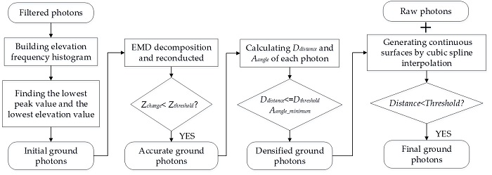
3.1. Noise Photon Removal
In this study, an improved localized statistics-based algorithm was proposed to filter out noise photons. There are two key steps to implement this algorithm. The first step is to build an elevation frequency histogram for removing the apparent noise photons. Another step is to establish the density distribution histogram for eliminating the remaining noise photons. An overview of the major steps is exhibited in Figure 1.
In the first step, a method based on an elevation frequency histogram was first introduced to roughly reduce the noise [28]. This method was performed as follows: (1) Grid-division: Dividing the raw data into partial bins of 200 m in the along-track direction and 20 m in the elevation direction, (2) building the elevation frequency histogram and then finding the bin at which the maximum frequency is located. The average elevation value of the bin is the location where the signal is concentrated, and (3) creating a buffer within 150 m above and below this location to contain all potential signal photons and remove the obvious noise photons. The parameters for this method were chosen based on a trial-and-error approach that worked efficiently for all MATLAS datasets.
The second step is intended to further remove the remaining noise photons. This step was performed as follows.
- (1)
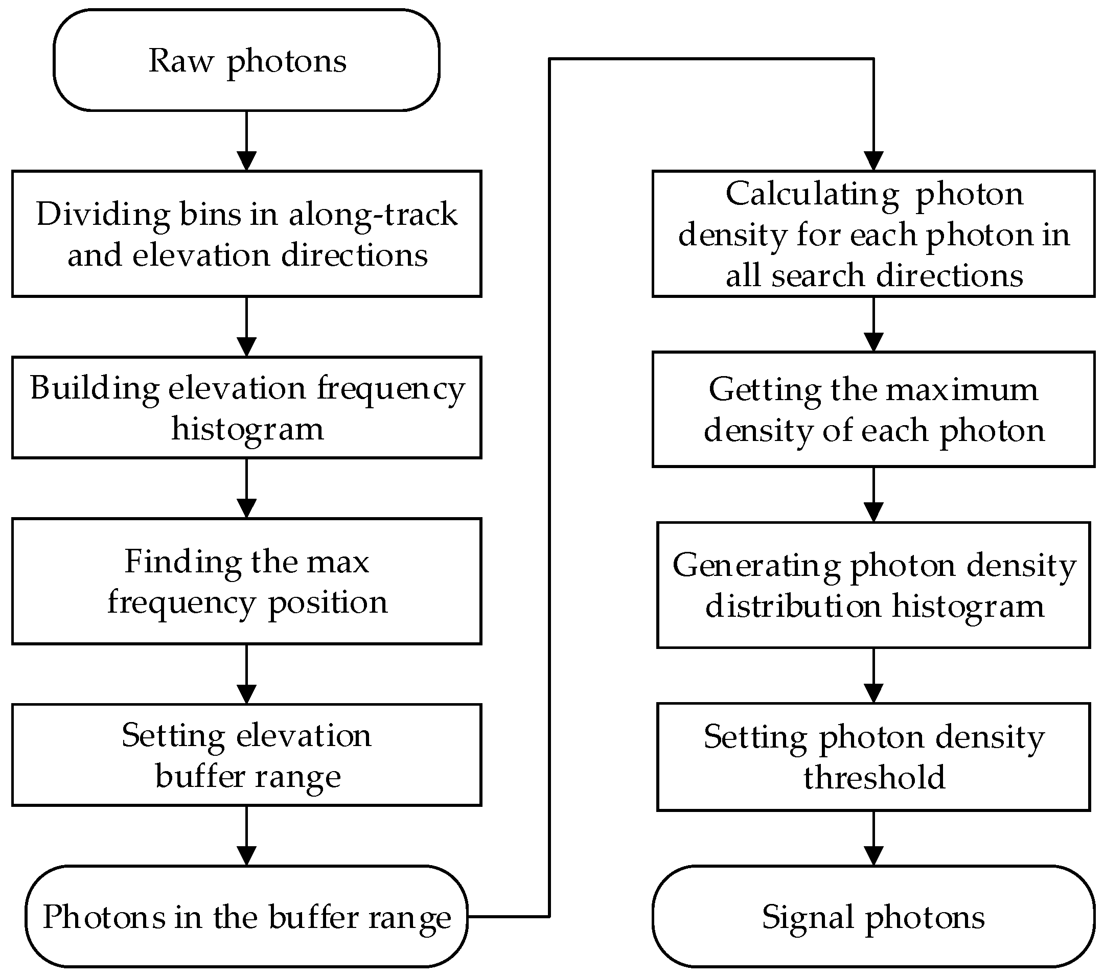
- Calculating the photon density of each photon, which is defined as the number of photons within its search area. Due to the grid division, there were no photons in the part of the search area of the photons located at the border region of the bin. Therefore, the densities of the photons within the border region were much smaller than those of photons located in the non-border region. To reduce the influence of edge effect, we used the method proposed by [27]. Firstly, the expanded bin was added in an adjacent area (red dotted frame in Figure 2) to reduce the edge effect in the along-track direction. The extended width is the semi major axis of the search area. Secondly, to reduce the edge effect in the elevation direction, the photons located in the upper and lower expanded bin border region were first detected and selected. Then according to the Equation (1), these detected photons were mirrored (green dotted frame in Figure 2). Finally, data filling was conducted using expanded bin and mirrored bin.
- (2)
- Getting the maximum density of each photon. A search ellipse was adopted to calculate the photon density according to previous studies [25,27,38,39]. As the distribution of photons is closely related to the terrain slopes, an ellipse relative to the surface slopes can be generated to achieve better density statistics [5]. However, terrain slopes over the raw photon-counting LiDAR data are unknown. In this paper, the photon density in each direction was calculated, and the maximum density value was taken as the final density value of each photon according to Xie [39]. The distance between two photons p(xp,zp) and q(xq,zq) is defined as Equation (2). The semi-major axis a and semi-minor axis b were set to 40 m and 4 m, respectively. If is less than 1, photon q is inside the search ellipse, else photon q is outside the search ellipse. By counting the number of photons within the search ellipse formed by photon p, the density of photon p in the direction is calculated. To increase the speed of the algorithm, the direction interval of the search ellipse is set to 5°, and the densities of each photon in 36 directions are calculated. Based on Equation (3), the maximum density was taken as the final density value of this photon. Figure 3 shows the final direction of the search ellipse formed by photon p, and its final density value is 8.
- (3)
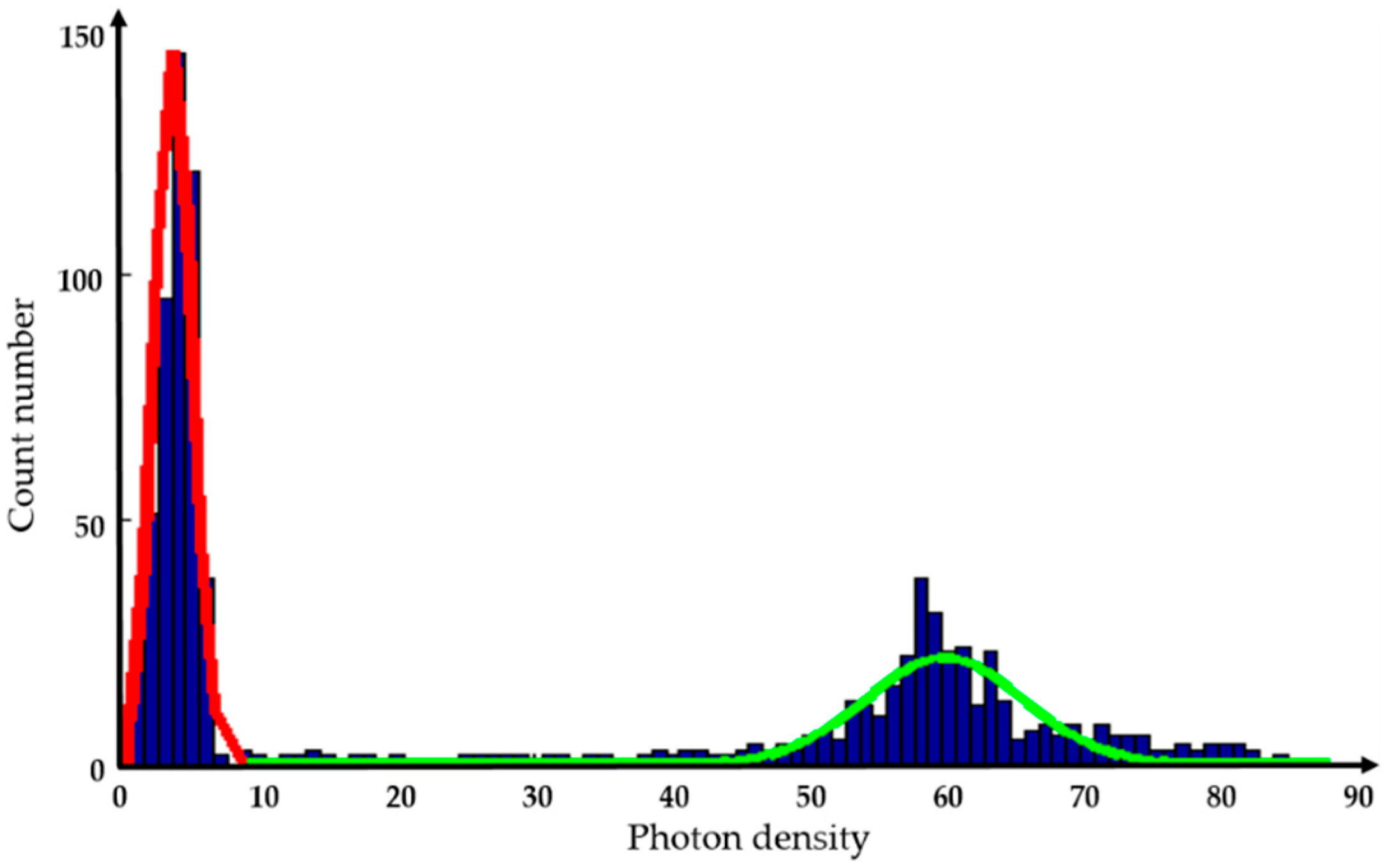
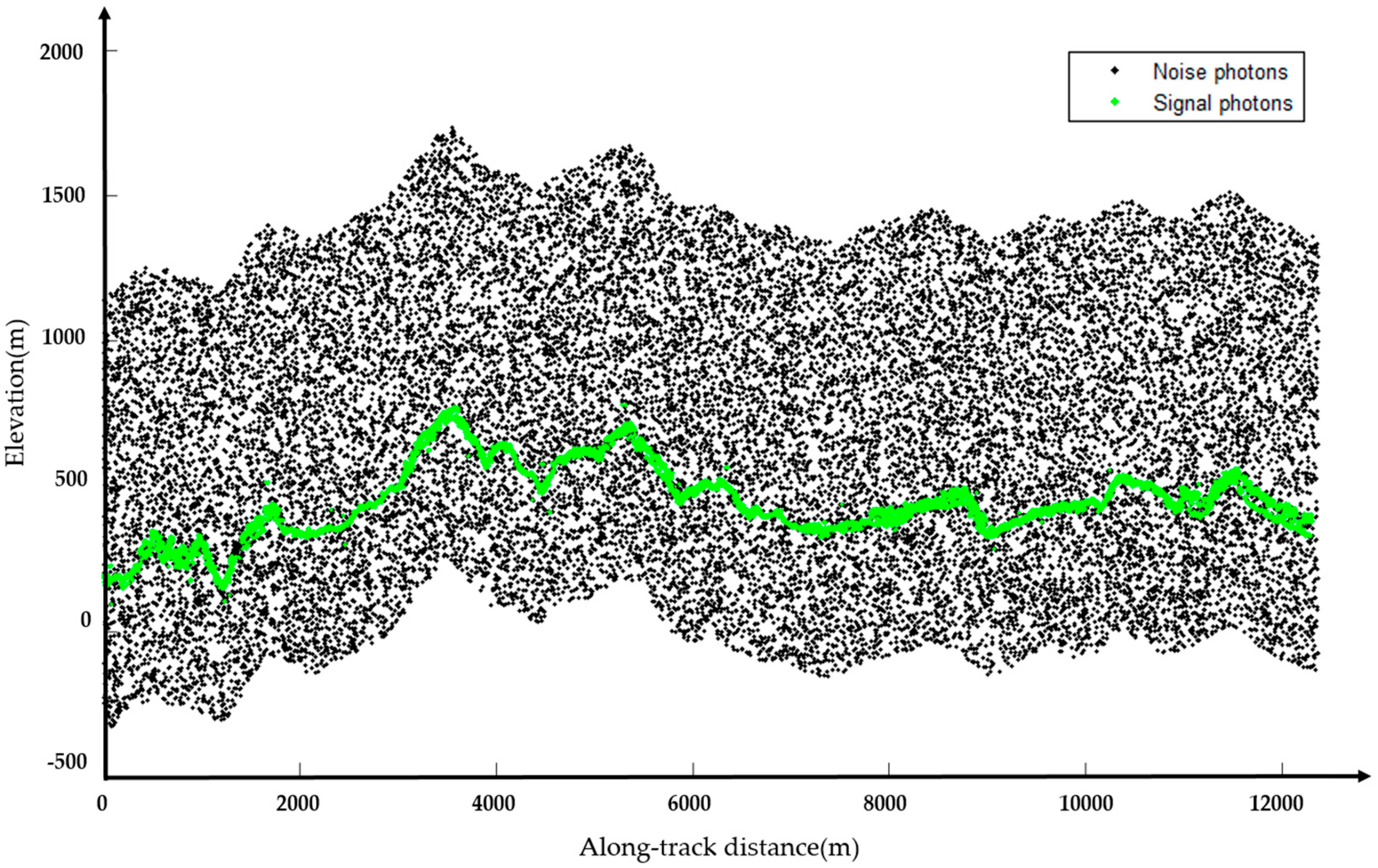
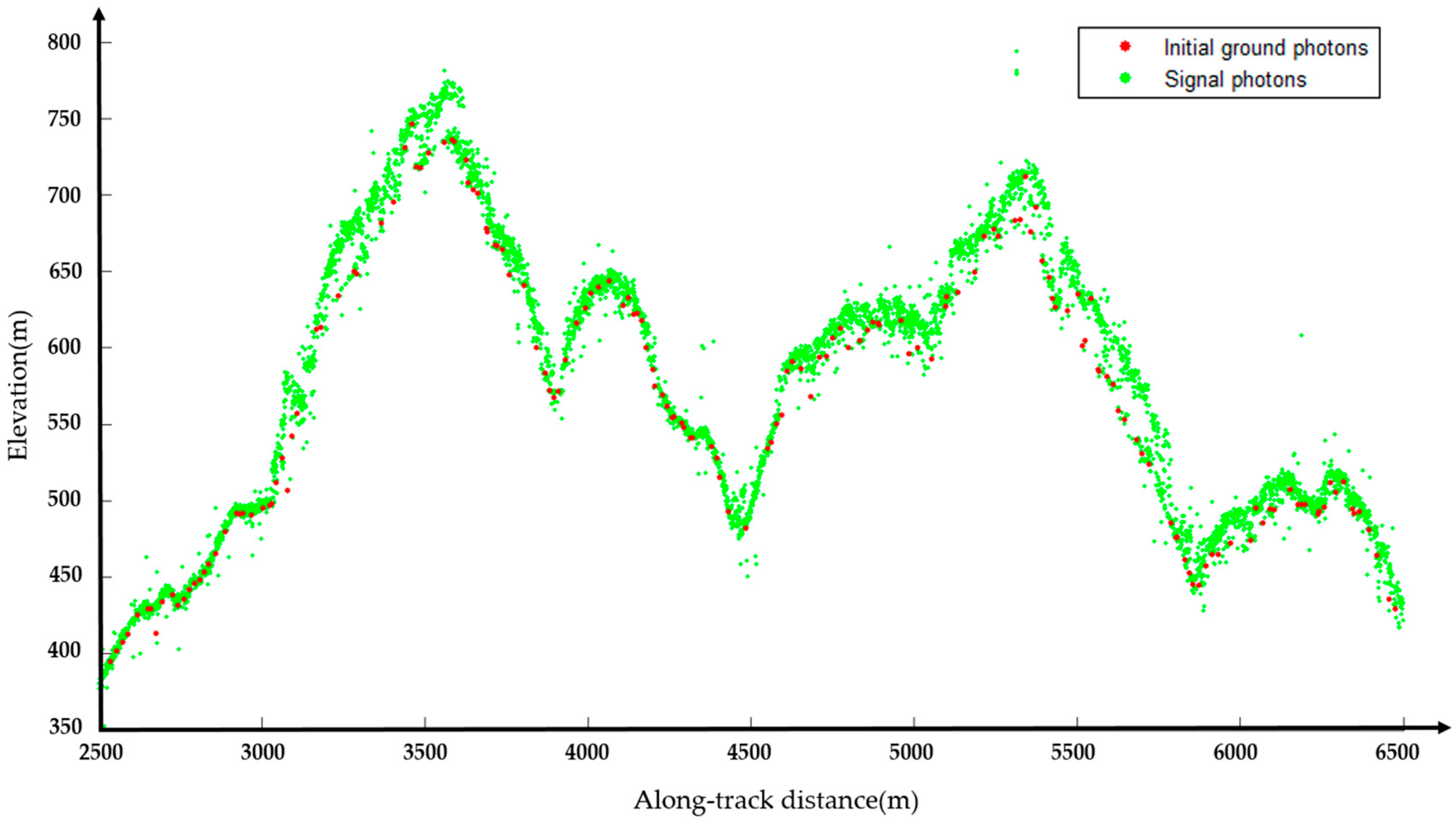
- Generating local photon density distribution histogram. It is well known that the density of a signal photon is much higher than that of a noise photon, and photons with low density can be regarded as noise photons. In this case, a photon density threshold must first be set to separate the signal photons from the noise photons. There are four key steps for threshold determination according to Land/VEG Science Definition Team (SDT) Team Members and ICESat-2 Project Science Office [40]. Firstly, all potential peaks of the histogram were detected by local maximum. The leftmost peak can be regarded as the noise peak because noise photons have lower photon density. Secondly, a Gaussian curve (red line in Figure 4) was fitted to the noise peak which was subsequently removed from the histogram via subtraction. Thirdly, the other Gaussian curve (green line in Figure 4) was fitted to the remaining histogram which is regarded as the signal Gaussian curve. Finally, the intersection of the two Gaussians determines the density threshold. Photons with final density value less than the threshold were classified into noise photons and subsequently removed from the raw photon-counting LiDAR data. The final possible signal photons (green) after the noise removal algorithm are shown in Figure 5.
3.2. Classification of Filtered Photon-Counting Data
According to previous studies, the filtered photons must be classified into ground and TOC photons to recover the ground and TOC surfaces and thereafter estimate the vegetation height. In this study, two algorithms are proposed to effectively identify ground and TOC photons.
3.2.1. Ground Photon Identification
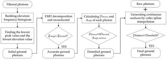
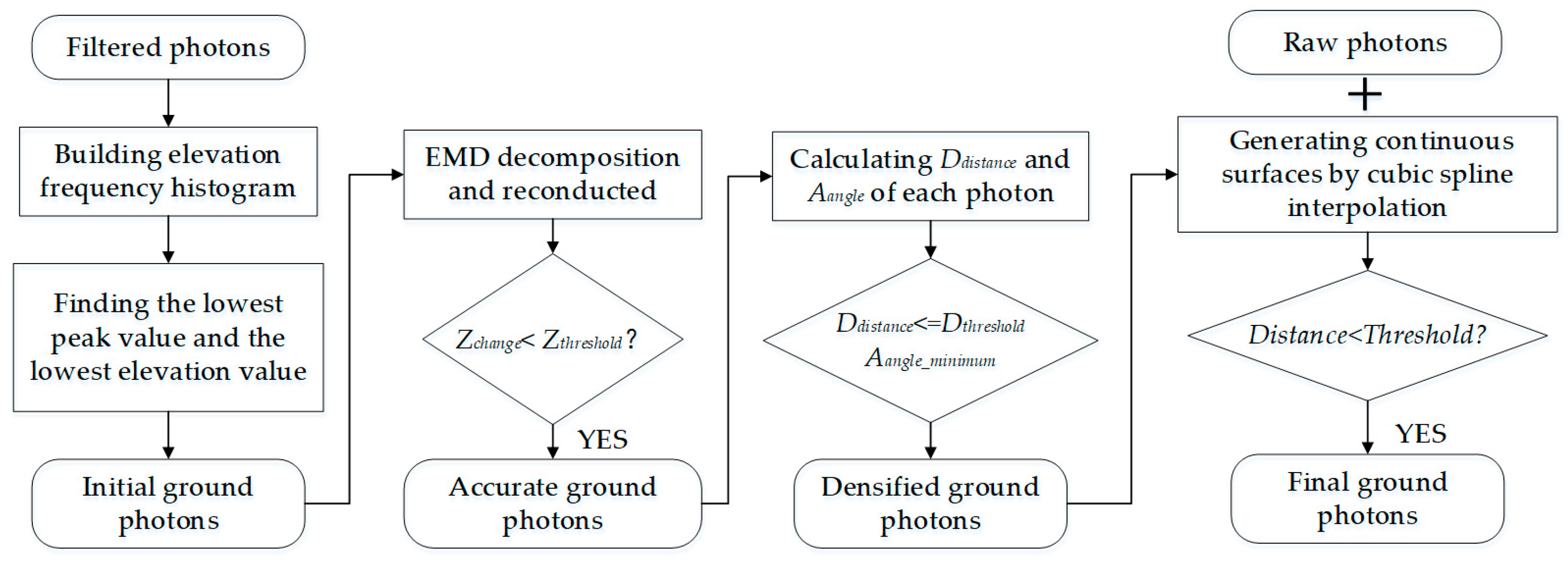
Identifying all potential ground photons is a necessary prerequisite for estimating ground elevation and vegetation height. In this study, an effective ground photon identification algorithm is proposed to extract ground photons and generate ground surfaces. The new algorithm consists of four steps: Extract initial ground photons by building an elevation frequency histogram, extract accurate ground photons using EMD, add the number of ground photons based on progressive densification, and generate ground surfaces utilizing cubic spline interpolation. An overview of the major steps is exhibited in Figure 6.
Initial Ground Photons Extraction
In previous studies, the initial ground photons were selected based on the assumption that the photon with the lowest elevation in each window belongs to the true ground surfaces. However, there are several noise photons around the ground that cannot be eliminated by the noise removal algorithm. In this case, the previous methods are not suitable for accurately extracting the initial ground photons. In this study, a new method for initial ground photons extraction was proposed and performed as follows: (1) Window division. The filtered photons were divided into windows in the along-track direction, and the window size was set to 15 m. (2) Building an elevation frequency histogram for each window. Photons of each window were layered according to the elevation value, and the layer thickness was set to 1 m. The photon frequency of each layer was calculated to build an elevation frequency histogram and then all the peaks are found in the histogram. (3) Extracting the initial ground photon based on the lowest peak value (LPV) of the elevation frequency histogram. While the LPV may not locate on the ground, it may be in the canopy or under the ground. In order to identify this kind of LPV, we compared the difference between the LPV and elevation value of the lowest photon. If the difference was less than the distance threshold 5 m, the LPV was defined as the ground peak, and the photon with the highest density in this layer was selected as the initial ground photon. Otherwise, the LPV is not corresponding to the ground surface. The lowest photon that satisfies the density threshold calculated by photon density distribution histogram in Section 3.1 was determined as the initial ground photon. The two parameters of the distance threshold and the density threshold are dependent on the experience judgment. The results of the initial ground photons extraction (red dots) are shown in Figure 7.
Accurate Ground Photons Extraction
The canopy photons or noise photons around the ground may be misclassified as the initial ground photons in the above step. These misclassified initial ground photons, denoted as pseudo-ground photons, must be eliminated because they may affect the identification of true ground photons. To reduce the effect of pseudo-ground photons, EMD was used to extract accurate ground photons.
EMD is a local, self-adaptive analysis and fully data-driven approach that is suitable to analyze nonlinear and nonstationary signals. It is widely used to remove noise points or mutation points from signals. By the EMD method, any signal can be adaptively decomposed into a series of intrinsic mode functions (IMFs) based on the local characteristic of the signal [41,42,43]. The IMFs are required to satisfy two conditions: (1) The number of extrema and the number of zero-crossings must either be equal or differ by no more than one; (2) the mean value of the envelope defined by the local maxima and the envelope defined by the local minima must be zero. The original signal is decomposed into a number of IMFs and a residual, as follows:
where stands for the decomposed IMF, n is the number of extracted IMFs, and represents the final residual.
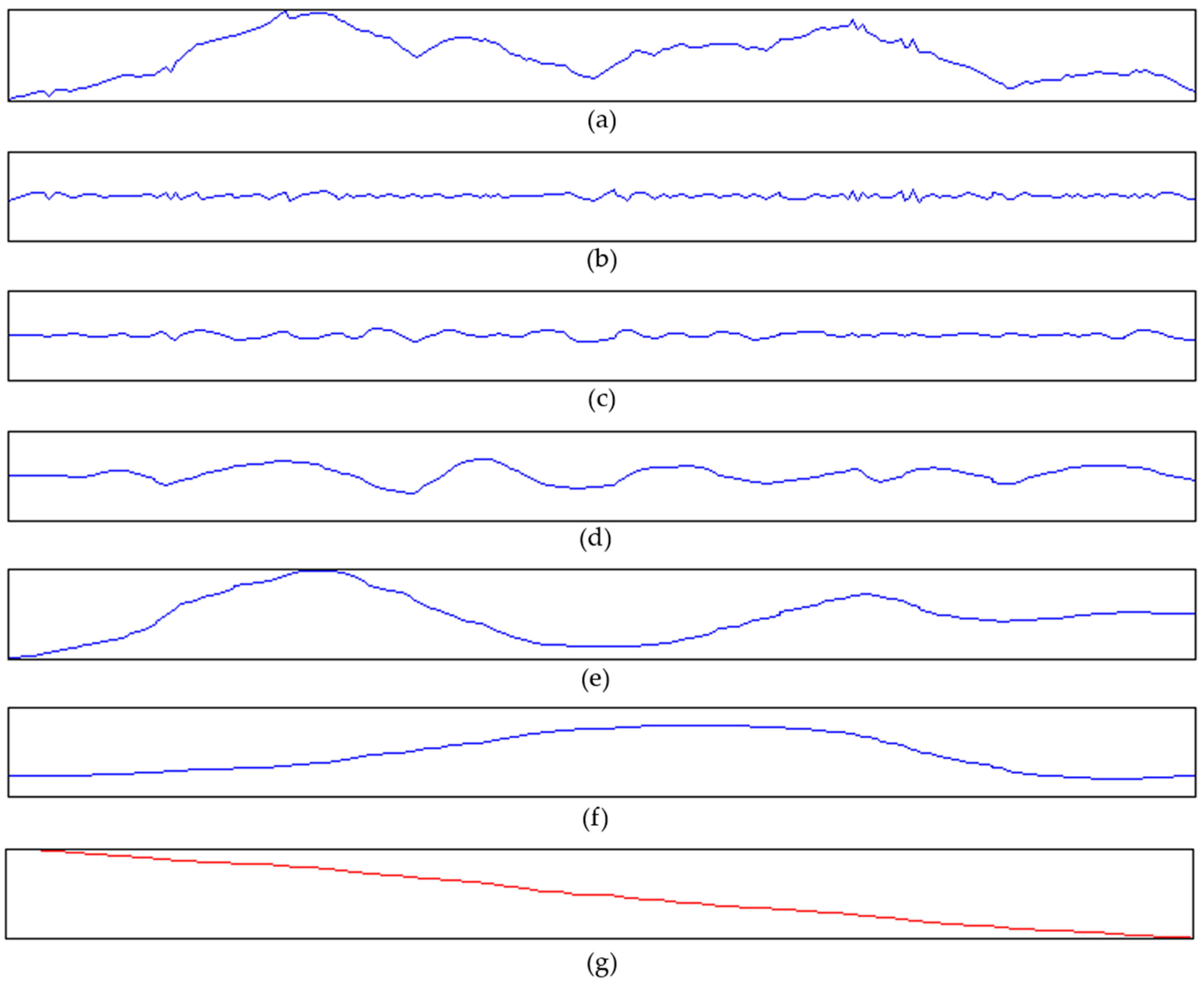
The decomposed IMFs consist of IMFs that primarily contain useful information and IMFs that carry noise. As shown in Figure 8b,c, the low-order IMF components obtained by the decomposition are high-frequency parts that usually contain noise and sharp parts of the data. The high-order IMF components are low-frequency parts, which are relatively less affected by noise and can be regarded as the useful signals (Figure 8e,f). Thus, there is a certain demarcation point k, which makes noise dominant in the first k IMFs and useful signals dominant in the subsequent IMFs. The demarcation point k is found by the method of Otsu. We assume that the first k IMFs and the final residual constitute the “foreground” class, and the subsequent IMFs and the final residual constitute the “background” class. According to Otsu, when the variance between the “foreground” class and the “background” class is the largest, the misclassification probability of the two classes is the smallest, and the k at this time is the optimal demarcation point. Then, the threshold is determined and applied to the first k IMFs according to Equations (5) and (6). All the IMFs are reconstructed, and the reconstructed result is shown in Equation (7). Finally, the elevation difference between the raw data and reconstructed data is calculated. If the difference is within the threshold of 1 m, it is a real ground photon; otherwise, it is a pseudo-ground photon. Through the above steps, accurate ground photons were obtained. The accurate ground photons and the erroneous ground photons are illustrated in Figure 9.
Progressive Densification of Ground Photons
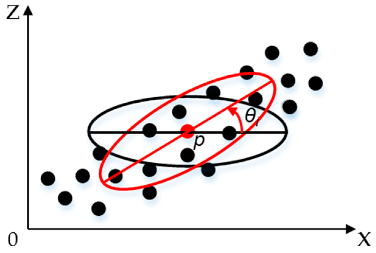
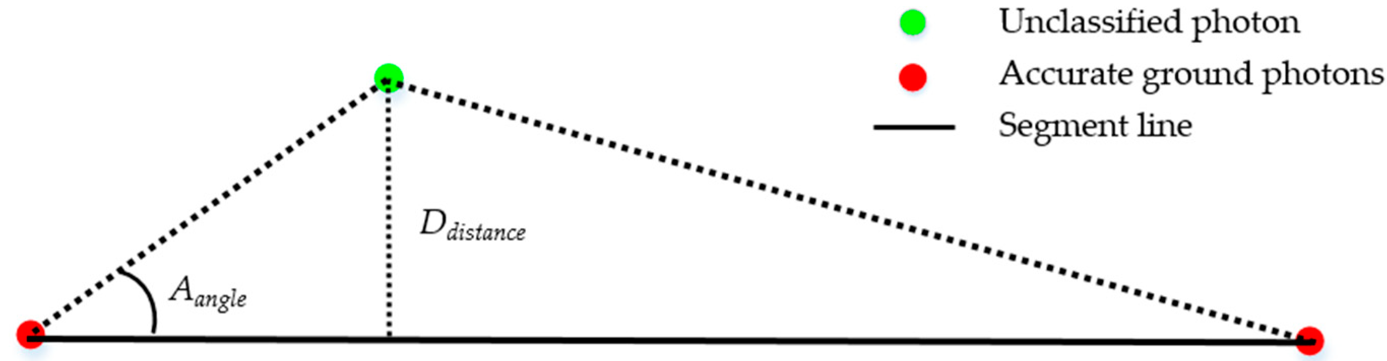
As few accurate ground photons are obtained in the aforementioned steps, a progressive densification method was proposed to increase the number of ground photons and improve the accuracy of the subsequent cubic spline interpolation. In this method, two parameters of the target classification photon (filtered photon which is unclassified) were calculated. The first parameter is the Ddistance, which is the distance from the target classification photon to the corresponding ground segment line. The second parameter is the Aangle which represents the angle between the ground segment line and the segment line comprised by the target classification photon and the closest accurate ground photon. The two parameters are shown in Figure 10.
All the photons whose Ddistance was less than the Dthreshold (1 m, determined by trial-and-error approach) was found, and the photon with the smallest Aangle was selected as the densified ground photon. Then, loop progressive densification was performed until no unclassified photon satisfies the condition. After four iterations, the number of densified ground photons was no longer increasing, and the final results are shown in Figure 11.
Establishment of Ground Surfaces
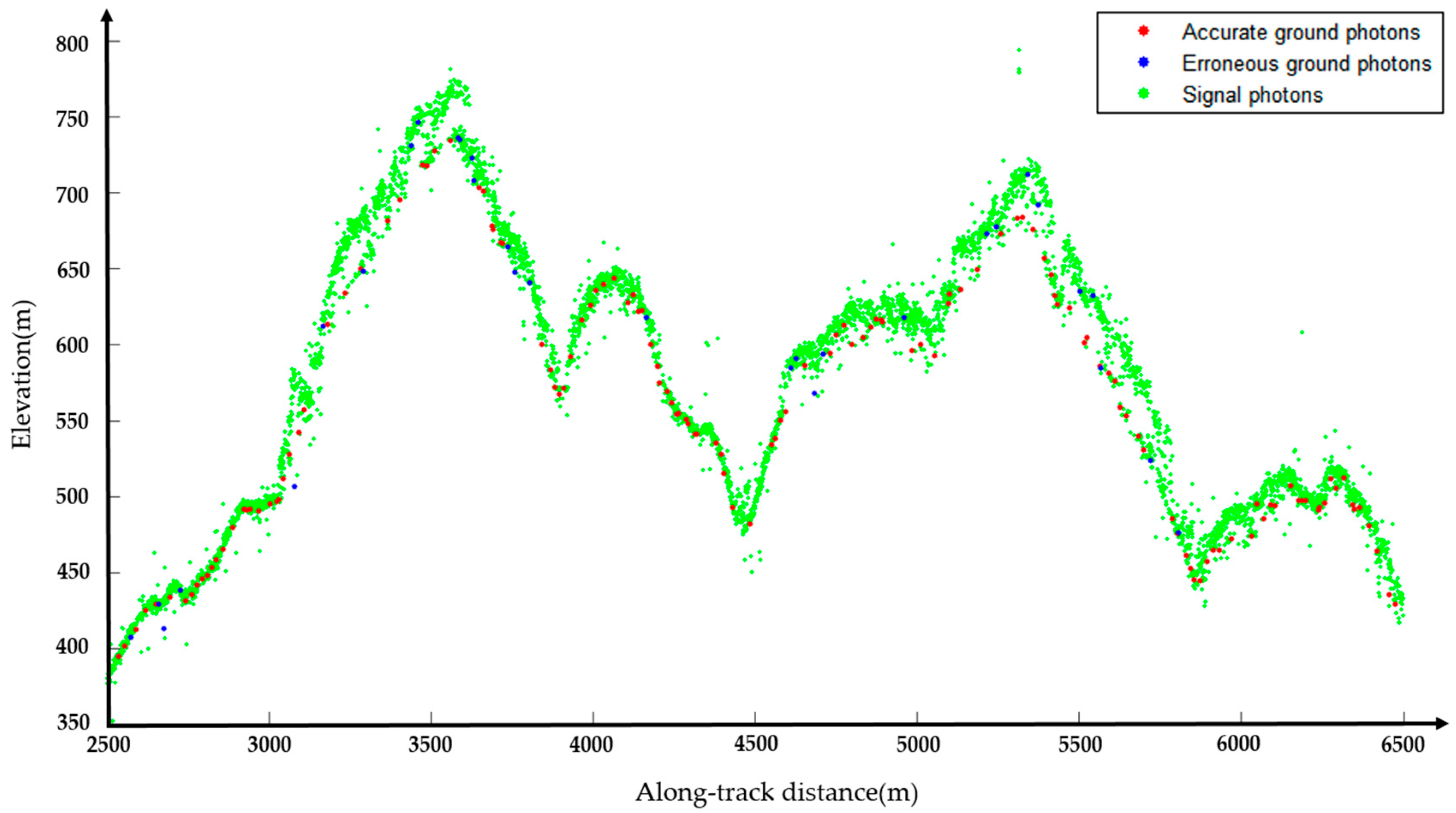
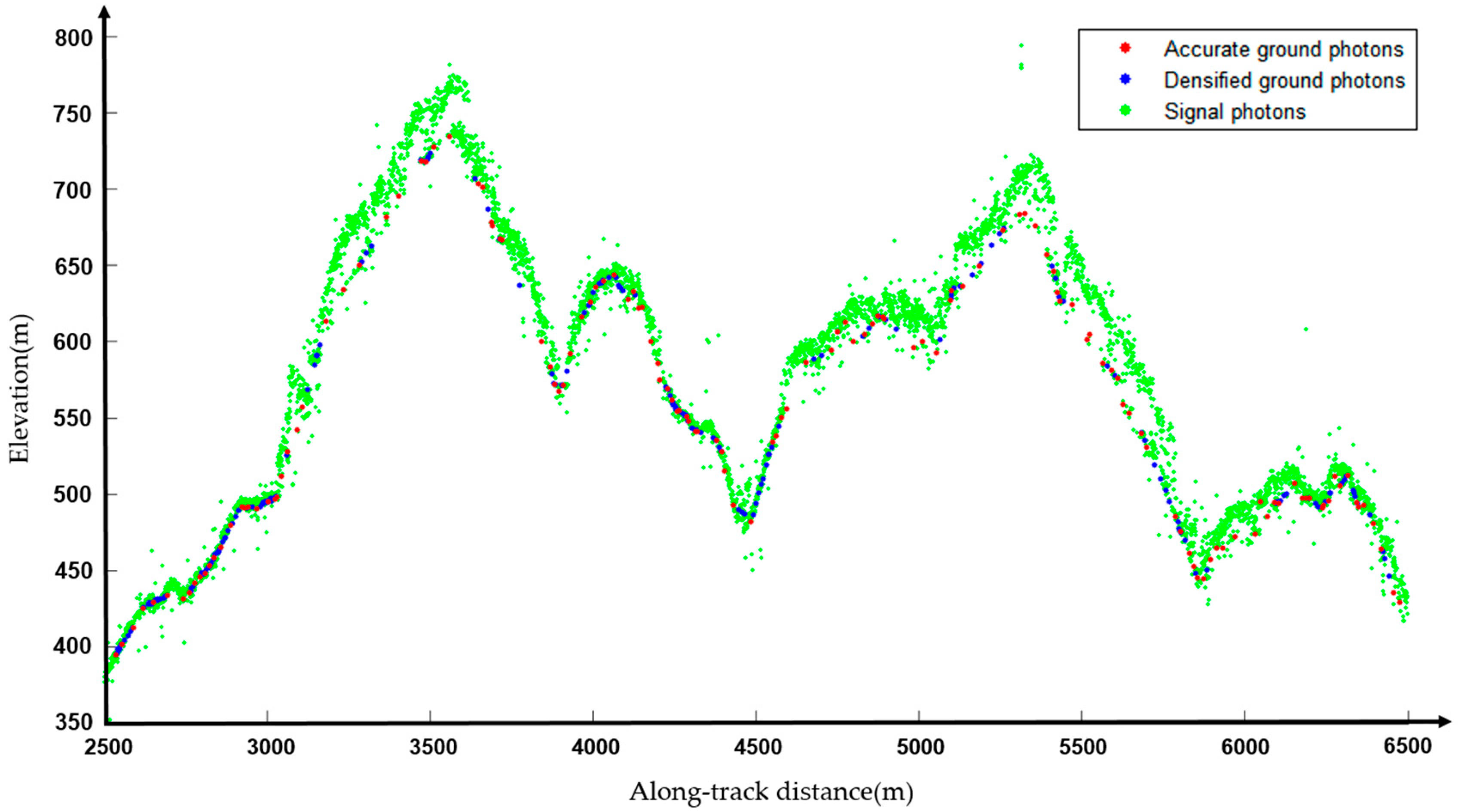
To establish the continuous ground surfaces, cubic spline interpolation was utilized to fit the ground photons. As the ground photons obtained in the previous steps are based on the filtered data, considering that some ground photons may be filtered as noise photons, we extracted the final ground photons from the raw photon-counting LiDAR data by received ground surfaces. If the distance between the raw photon and the ground surfaces is within the threshold of 1 m, it was classified as a ground photon. Finally, all ground photons were extracted from the raw photons. The ground surfaces and the final ground photons are shown in Figure 12.
3.2.2. TOC Identification
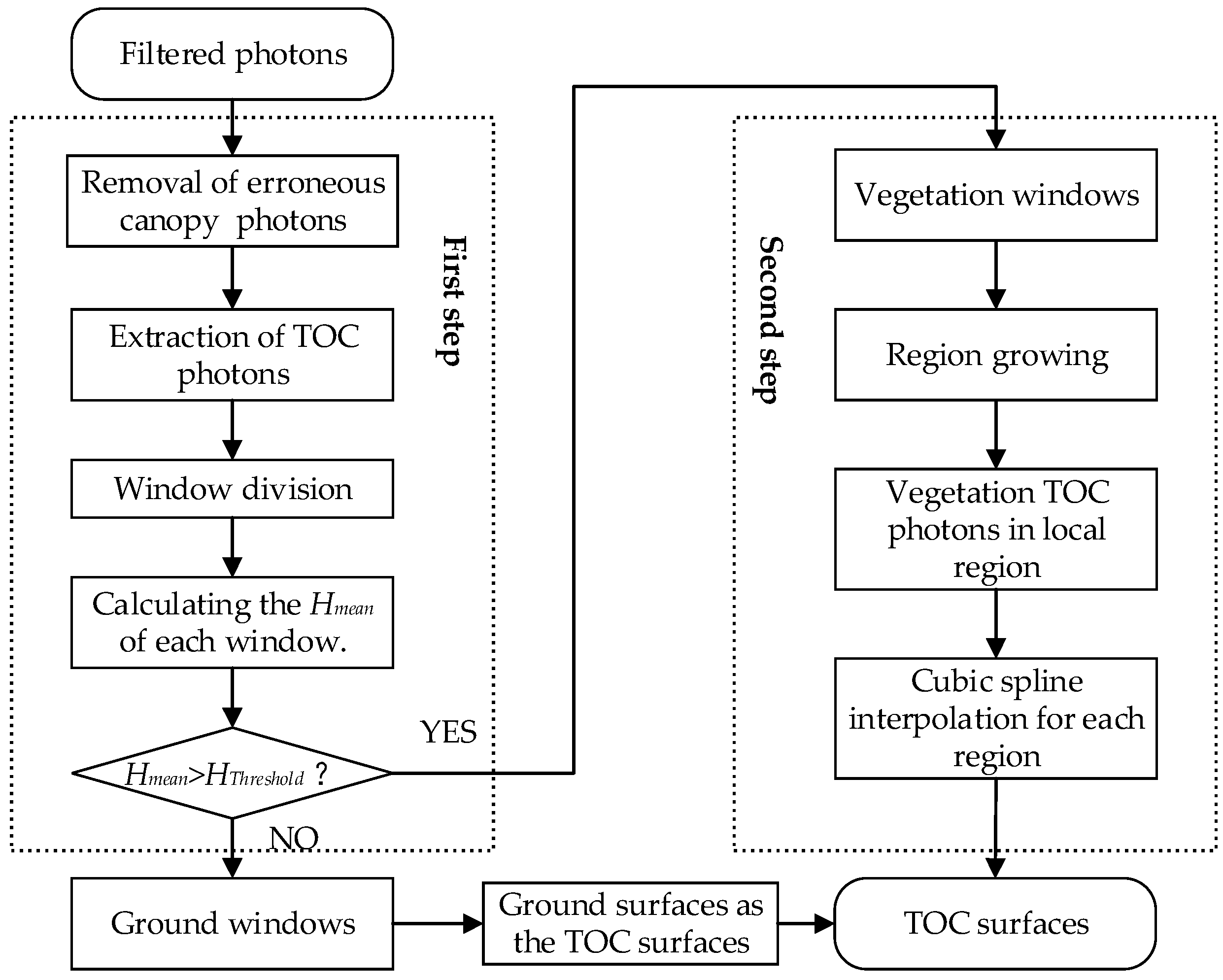
It is well known that the TOC surfaces are not smooth. Thus, the algorithm for extracting ground photons is not suitable for TOC identification. An effective TOC identification algorithm was proposed to extract TOC photons and recover TOC surfaces. The new algorithm consists of two steps. The first step is to extract the TOC photons in each window and classify the windows into ground and vegetation by mean tree height (Hmean). The second step is to grow regions for vegetation and ground windows and generate local TOC surfaces utilizing cubic spline interpolation for each region. The final TOC surfaces are the local ground surfaces of the ground regions and the local TOC surfaces of the vegetation regions. An overview of the major steps is exhibited in Figure 13.
TOC Photons Extraction and Classification
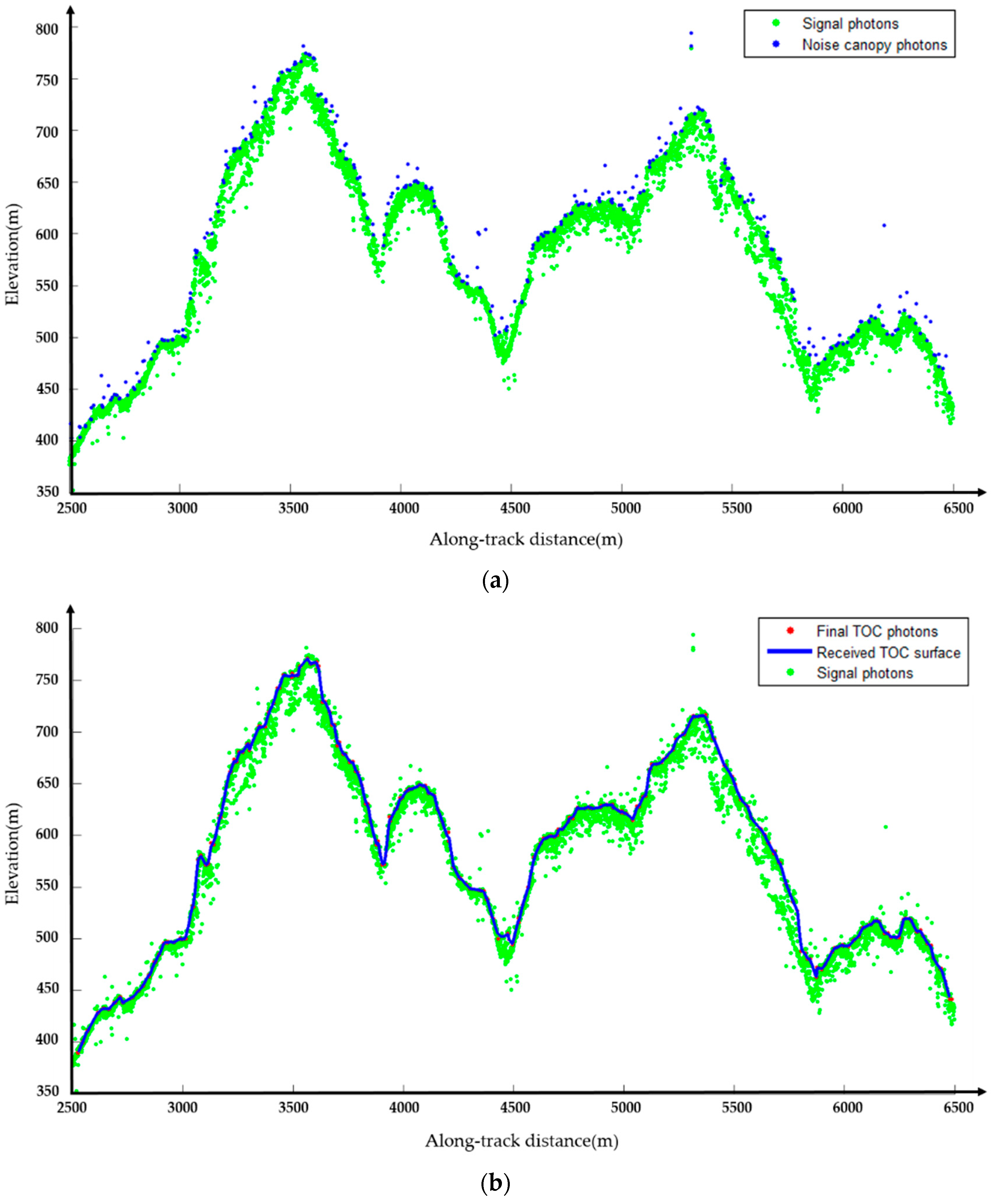
The TOC photons were extracted by the method proposed by Popescu et al. [26], and the method consists of two essential steps. (1) Removing erroneous canopy photons. For each window, the photons within a specified elevation quantile range [0.96, 1] for the daytime data and [0.99, 1] for the nighttime data were assumed to be the possible noise photons and were removed. The erroneous canopy photons are shown in Figure 14a. (2) Obtaining the possible TOC photons within the quantile range [0.95, 0.99] using the remaining photons. To generate TOC surfaces, Popescu et al. [26] utilized cubic spline interpolation to fit the possible TOC photons directly. However, the results were inaccurate because of the large elevation difference between the TOC photons and the ground photons. To solve this problem, we divided the data into vegetation areas and ground areas before cubic spline interpolation. The process was performed as follows. (1) Window division. The possible TOC photons were divided into 20 m windows in the along-track direction. (2) Calculating the Hmean of each window by the obtained ground surfaces and possible TOC photons. (3) Classifying the windows into vegetation and ground by Hmean. We found that the canopy height was always greater than 2 m in the vegetation area by analyzing the characteristic of all MATLAS datasets, thus the vegetation area and the ground area can be classified by the HThreshold of 2 m. If the Hmean of a window is greater than the HThreshold, it is classified into the vegetation window. Otherwise, it is classified into the ground window.
Establishment of TOC Surfaces
Windows have been classified into ground windows and vegetation windows in the above step. The next step is to generate TOC surfaces. For vegetation windows, a region growing algorithm was first used to join adjacent windows into a region, then the cubic spline interpolation was utilized to generate continuous TOC surfaces by fitting the possible TOC photons for each region and all TOC photons were finally extracted from the raw photon-counting LiDAR data. For the ground windows, the obtained ground surfaces were used as pseudo TOC surfaces. We extracted all the TOC photons and built TOC surfaces by local TOC surfaces and ground surfaces. The final TOC surfaces are shown in Figure 14b.
3.2.3. Vegetation Height Retrieval
Once the ground surfaces and canopy surfaces are recovered, vegetation height is the elevation difference of the two and can be obtained at any position in the along-track direction. In this paper, vegetation height was calculated in each 20 m window in the along-track direction.
3.3. Accuracy Assessment
In this study, the DTM and CHM derived from airborne LiDAR data were used to assess the accuracies of ground elevation and vegetation height, respectively. The geolocation precision of 2014 MABEL was 30 m root-mean-square error (RMSE) described by [44], but this figure was derived after significant engineering improvements had been made to MABEL and errors for our 2012 data were likely to be larger. To minimize the geolocation error of MABEL data, effective methods have been proposed and verified by Popescu et al. [26] and Gwenzi et al. [29]. As MATLAS data was generated from MABEL data, these methods can be used for MATLAS data. These methods consist of two essential steps. Firstly, shifting the ground photons classified from MATLAS data in the x and y direction and then determining the best shift that resulted in the lowest RMSE error between ground photons and the corresponding reference DTM data. Secondly, further adjusting the elevation of MATLAS data by adding the elevation difference between the two with the highest frequency. Subsequently, the mean difference (MD), the standard deviation (SD) and RMSE between the estimated data (the ground elevation and vegetation height) and the corresponding reference data were calculated to quantify the performances of our algorithm. Additionally, to further verify the applicability of our algorithm, this study conducted a comparison between our algorithm (Algorithm 1) and a commonly used algorithm (Algorithm 2) proposed by [28].
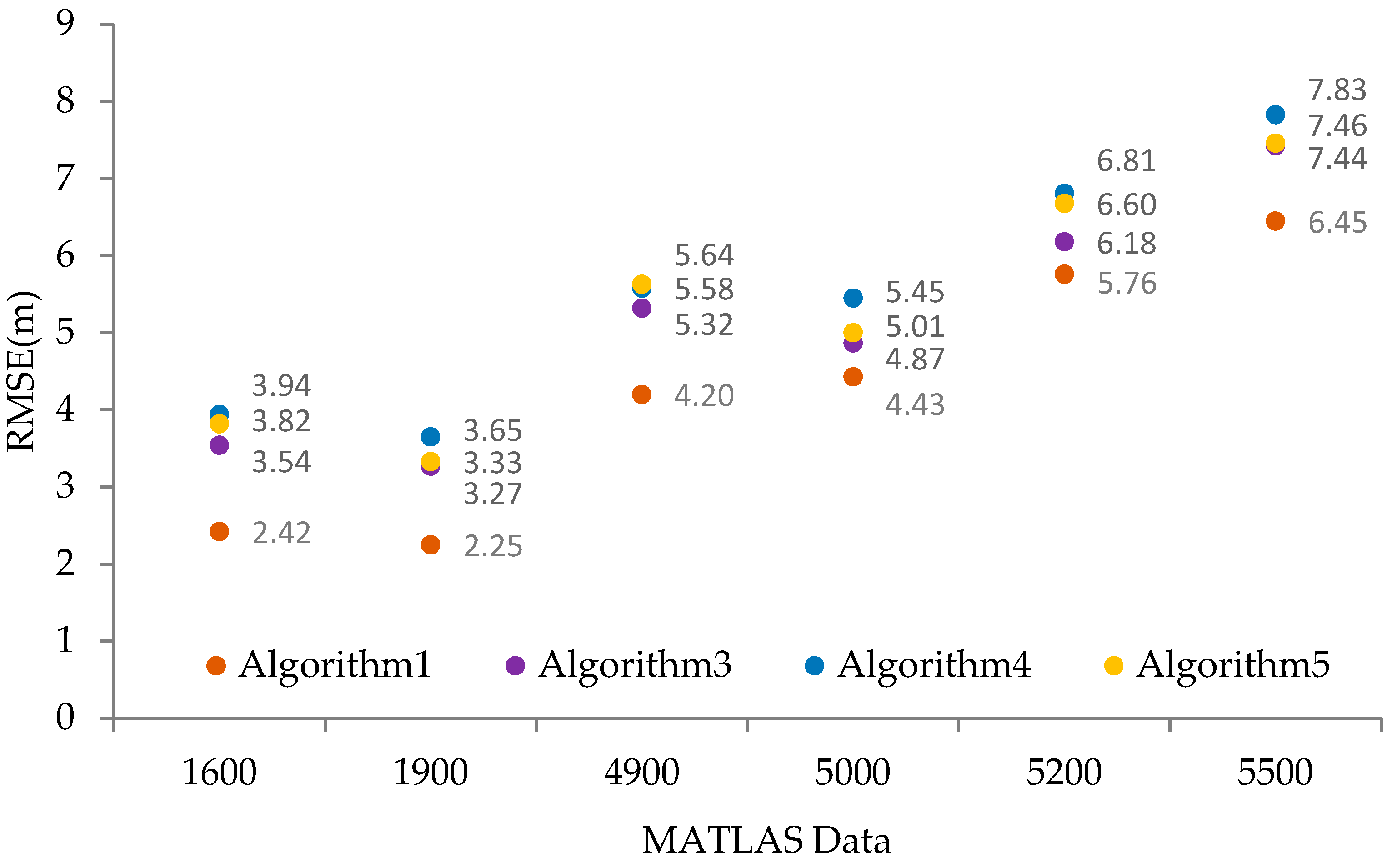
As indicated in Section 3.2.1, our ground photon identification algorithm consists of four steps. The last step of establishing ground surfaces utilizing cubic spline interpolation is indispensable. To verify the influence of the first three steps on the ground identification algorithm, three algorithms referred to as Algorithm 3, Algorithms 4 and 5, were established. Algorithm 3 took the photon with the lowest elevation as the initial ground photon in the first step to test the influence of LPV. Algorithm 4 did not use the EMD method in the second step. Algorithm 5 skipped the progressive densification method in the third step. The MD, SD and RMSE between the estimated data (the ground elevation) and the DTM were calculated to verify the performances of the first three steps of ground photon identification algorithm.
4. Results and Discussion
4.1. Noise Removal
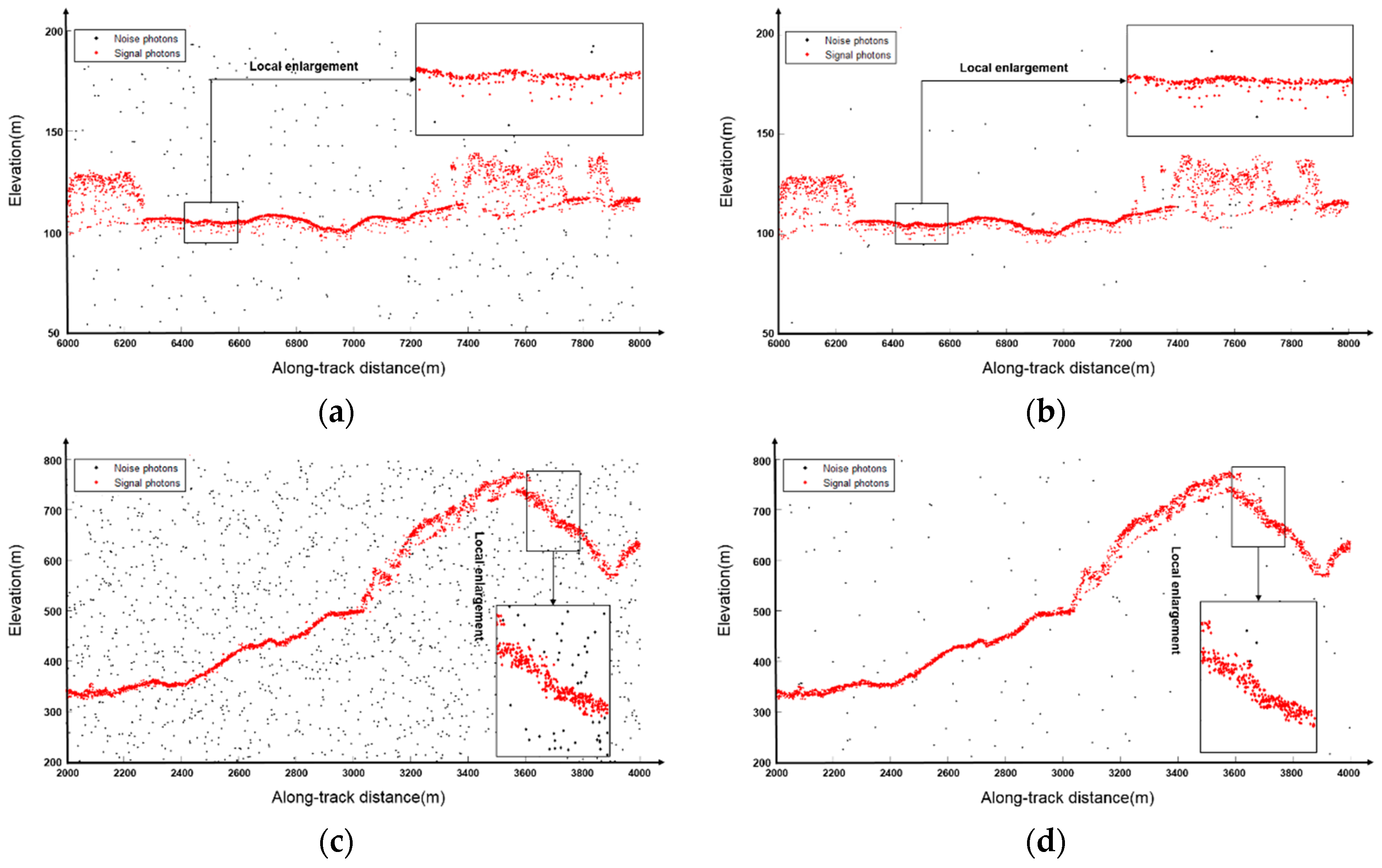
The profile of signal photons is reliably extracted from raw photons by our noise removal algorithm shown in Figure 15. The red dots represent signal photons, and the black dots represent noise photons. The black box displays the local enlargement part of each profile. Additionally, Figure 15a,b shows the results of hilly areas in daytime and nighttime, respectively. Figure 15c,d reveals the results of the mountain area in the daytime and nighttime, respectively. By comparing Figure 15a–d, we found that most of the noise photons were removed by our algorithm, and nighttime data achieved better performance results than daytime data because of the high signal-to-noise ratio (SNR). By considering the directionality of the photons, the possible signal photons can be well preserved, especially in the areas with steep terrain as shown in Figure 15c,d. Both ground photons and vegetation photons are retained completely regardless of the terrain slopes. However, there are some photons around the ground, which are difficult to remove, as shown in Figure 15a,b. These photons will be removed by our photon classification algorithm.
4.2. Photon Classification
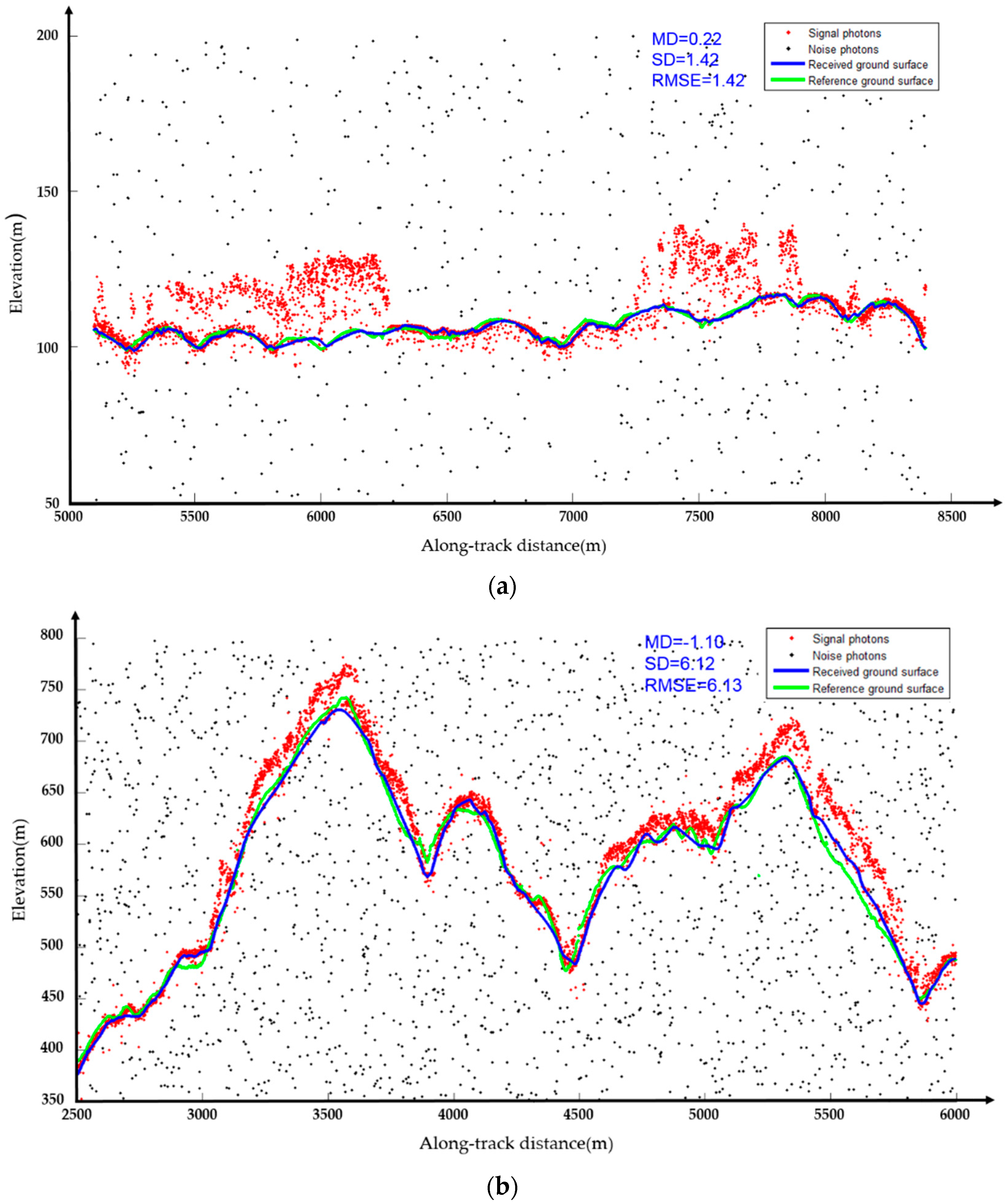
A qualitative analysis was conducted by comparing the received ground surfaces and reference DTM surfaces. Figure 16a,b demonstrates an example of retrieved ground surfaces with corresponding descriptive statistics in the East Coast with hills and West Coast with mountains, respectively. The retrieved ground surfaces in the hilly area are potentially close to the reference DTM surfaces in either the vegetation or bare land areas. While in the West Coast with mountains, there are several places where the ground surfaces are far from the reference DTM surfaces. For example, in the area between 5400 and 5700 m, there are no ground photons, so the extracted initial ground photons are actually canopy photons. Since there are no ground photons at a long distance, these canopy photons cannot be removed by EMD, resulting in errors. However, as long as there are ground photons, the results of ground photons extraction are very satisfactory. For example, in the area between 3050 and 3500 m, although there are few ground photons under dense vegetation, most of the extracted initial ground photons are real ground photons. Then, the canopy photons and the near-ground photons are removed by EMD. Finally, the ground surfaces are very close to the reference data. This observation is further confirmed by a smaller RMSE value of the retrieved ground in the hilly area (1.42 m) than in the mountain area (6.13 m). Other MATLAS datasets were also investigated, and the validation results are summarized in Table 2.
A quantitative ground elevation accuracy assessment of Algorithms 1 and 2 is summarized in Table 2. We did not provide results for Virginia because there are few available DTM data that could be used for validation. Table 2 indicates that both algorithms perform better on the East Coast than on the West Coast. By analyzing the characteristics of the MATLAS data, we found that the vegetation coverage and terrain slope in the West Coast are larger than that in the East Coast, which leads to the data quality of the West Coast being worse than that of the East Coast. There are daytime and nighttime data for the same area of the MATLAS data. According to Table 2, the RMSE values of both algorithms are lower in the daytime than in the nighttime for all datasets. However, there is little difference between the RMSE values of the two. This means that the difference of the signal photons separated by the noise removal algorithm between the daytime and nighttime MATLAS data is very small, which indirectly proves that the noise removal algorithm is effective.
From Table 2, we can see that the RMSE values of Algorithm 1 are lower than those of Algorithm 2 for all datasets. This may be explained by the two following reasons. (1) Algorithm 2 selects the lowest photon in each 10 m-diameter footprint as the initial ground photons, without considering the noise photons around the ground that cannot be eliminated by the noise removal algorithm. In contrast, our algorithm effectively reduces the influence of noise photons around the ground by utilizing the LPV of the elevation frequency histogram. (2) Cubic spline interpolation in an iterative manner is applied directly to the initial ground photons in Algorithm 2. To improve the accuracy of the cubic spline interpolation, our algorithm adopts EMD to remove the misclassified photons in the initial ground photons and increases the number of ground photons using the progressive densification method.
Our algorithm proved to achieve a better performance compared to Algorithm 2. To further verify the influence of the first three steps on the ground identification algorithm, the MD, SD and RMSE values of Algorithms 3–5 were calculated. Considering that the difference of RMSE values between the daytime and nighttime data is small, only the daytime data was used here. The results are summarized in Table 3 and Figure 17. As expected, Algorithm 1 outperformed Algorithms 3–5 from the perspective of the SD and RMSE values. Among the three algorithms, Algorithm 4 is prone to getting the largest SD and RMSE values for all datasets, which indicates that the EMD has the greatest impact on our algorithm. Better performance results are observed using Algorithm 3 compared with Algorithm 5, which indicates that the progressive densification method has a greater impact on our algorithm than LPV.
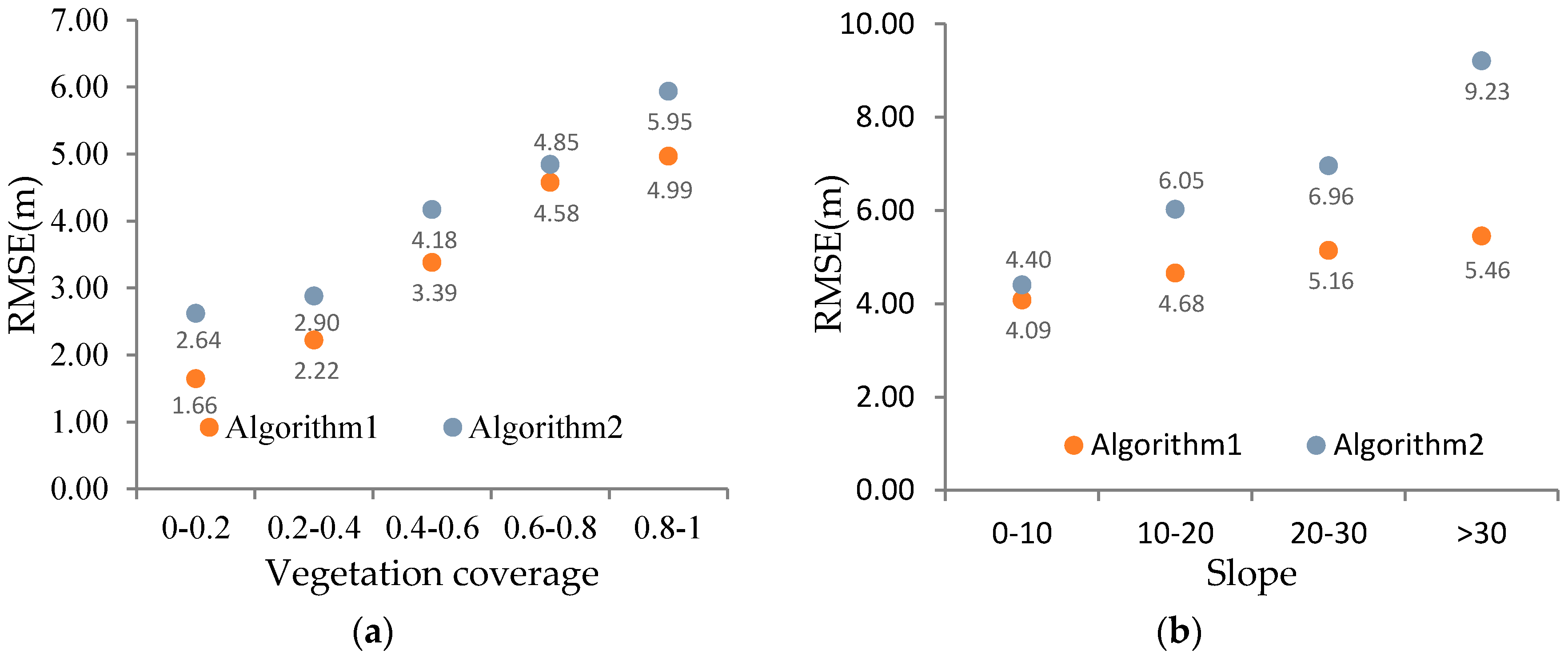
Vegetation coverage and surface slopes present the main challenges for identifying ground and TOC photons. To further explore the effect of vegetation coverage and surface slopes on ground surfaces extraction, the vegetation coverage and surface slope values of all the MATLAS data were graded, and the corresponding MD, SD and RMSE values of Algorithms 1 and 2 of each grade were calculated. The statistical results shown in Table 4 and Figure 18 indicate that the SD and RMSE values increase as vegetation coverage and slope levels increase. The results of Algorithm 1 are better than those of Algorithm 2 for all vegetation coverage levels, especially in 0–0.2 and 0.8–1. This may be because there are some noise photons around the ground in the vegetation coverage of 0–0.2, and the LPV method reduces the influence of these photons effectively. Some initial ground photons are canopy photons in the vegetation coverage of 0.8–1, and these photons can be removed by EMD to obtain accurate ground photons. Additionally, as the slope increases, the SD and RMSE value differences between the two algorithms increase obviously which indicate Algorithm 1 reduces the influence of the surface slopes effectively compared to Algorithm 2.
4.3. Vegetation Height Estimation
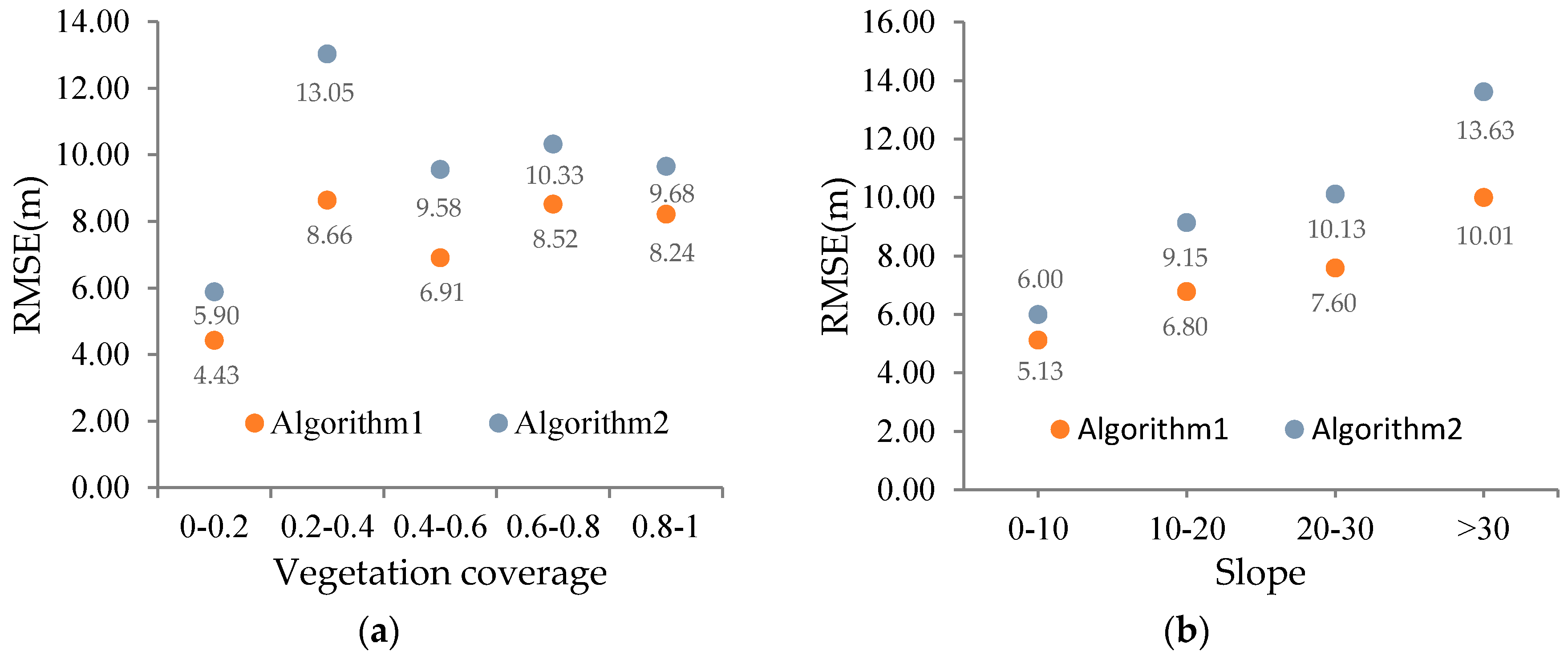
A quantitative vegetation height estimation accuracy assessment of Algorithms 1 and 2 is summarized in Table 5. As expected, the SD and RMSE values of vegetation height are larger than those of the ground surfaces because the vegetation height estimation is affected not only by ground surfaces but also by TOC surfaces. To better compare the accuracy of TOC surfaces extracted by Algorithms 1 and 2, the vegetation height in Algorithm 2 was calculated using the ground surfaces retrieved by Algorithm 1. Table 5 shows that the SD and RMSE values of vegetation height retrieved by Algorithm 1 are lower than that retrieved by Algorithm 2 for all datasets, which means that the accuracy of the TOC surfaces retrieved by Algorithm 1 is higher than that retrieved by Algorithm 2. The main reason may be that Algorithm 1 improves the accuracy of cubic spline interpolation by classifying data into vegetation and ground regions. Table 6 and Figure 19 provide a summary of the MD, SD and RMSE values of the retrieved vegetation height in different vegetation coverage levels and surface slope levels. From Table 6 and Figure 19a, we can see that the RMSE values of Algorithm 1 are reduced in all vegetation coverage levels, especially between 0.2 and 0.4. We can also see that the RMSE value differences increase with increasing slopes, as shown in Figure 19b, which means that Algorithm 1 also reduces the influence of the surface slopes on TOC surfaces.
Table 5 also reveals that the estimated vegetation height over the East Coast has lower SD and RMSE values than those of the West Coast. One reason is that the accuracy of the retrieved ground surfaces over the East Coast is higher than that of the West Coast. The second reason is the accuracy of the retrieved TOC surfaces. Better performance results of TOC surfaces are expected when the vegetation is distributed densely, and the terrain is mostly flat. The vegetation on the West Coast is distributed densely, and the terrain is steep. In contrast, many vegetation areas of the East Coast are distributed sparsely, and the terrain is flat. Therefore, the accuracy of the retrieved TOC surfaces between the West Coast and the East Coast is uncertain. The RMSE value differences of the TOC surfaces extraction by Algorithms 1 and 2 between the West Coast and the East Coast are small as shown in Table 5. Therefore, the SD and RMSE value differences of the vegetation height between the West Coast and the East Coast are mainly caused by the retrieved ground surfaces.
5. Conclusions
ICESat-2 will acquire synoptic measurements of vegetation canopy height, density, the vertical distribution of photosynthetically active material, leading to improved estimates of forest biomass, carbon, and volume in a wide area. In this paper, an automatic algorithm was proposed to accurately retrieve ground elevation and vegetation height from photon-counting LiDAR data. This automatic algorithm introduces a localized statistics-based noise removal algorithm and proposes a new photon classification algorithm. Based on the validation results of the ground elevation and vegetation height, we come to the following conclusions. (1) The noise removal algorithm reduces the influence of edge effect and photon directionality, and therefore, removes the noise photons and maintains the signal photons effectively; (2) the new ground identification algorithm is effective for extracting ground photons and retrieving ground elevation by carrying out a series of operations, including LPV, EMD, progressive densification and cubic spline interpolation; (3) the TOC identification algorithm is effective for extracting TOC photons by utilizing percentile statistics method and retrieving TOC surfaces by classifying TOC photons into vegetation areas and ground areas, and then utilizing cubic spline interpolation respectively; (4) our algorithm performs better than previous algorithms in retrieving ground elevation and vegetation height because it effectively reduces the negative impacts of surface slopes and vegetation coverage.
To summarize, our new proposed algorithm can provide a valuable basis for estimating ground elevation and vegetation height using photon-counting LiDAR data. However, in areas with dense vegetation, the emitted pulses may not penetrate the vegetation canopy and reach the ground surfaces, which make noise removal and photon classification challenging and subsequently limit the estimation accuracy of ground elevation and vegetation height. Therefore, our next study should focus on the development of a more effective noise removal algorithm and photon classification algorithm that can be applied even in areas with dense vegetation. Additionally, we can incorporate ICESat-2 data with other data, such as optical images, airborne LiDAR, radar and upcoming GEDI data, to expand their potential applications and increase the accuracy of the estimated parameters.
Author Contributions
C.W., X.Z. and S.N. designed the experiments; X.Z. and S.N. analyzed the data and wrote the paper; X.X. and Z.H. revised the paper.
Funding
This research was funded by National Natural Science Foundation of China, grant number 41671434.
Conflicts of Interest
The authors declare no conflict of interest.
References
- Zhang, G.; Ganguly, S.; Nemani, R.R.; White, M.A.; Milesi, C.; Hashimoto, H.; Wang, W.; Saatchi, S.; Yu, Y.; Myneni, R.B. Estimation of forest aboveground biomass in california using canopy height and leaf area index estimated from satellite data. Remote Sens. Environ. 2014, 151, 44–56. [Google Scholar] [CrossRef]
- Chen, Q. Retrieving vegetation height of forests and woodlands over mountainous areas in the pacific coast region using satellite laser altimetry. Remote Sens. Environ. 2010, 114, 1610–1627. [Google Scholar] [CrossRef]
- Kelly, M.; Su, Y.; Di Tommaso, S.; Fry, D.; Collins, B.; Stephens, S.; Guo, Q. Impact of error in lidar-derived canopy height and canopy base height on modeled wildfire behavior in the Sierra Nevada, California, USA. Remote Sens. 2017, 10, 10. [Google Scholar] [CrossRef]
- Neuenschwander, A.; Magruder, L. The potential impact of vertical sampling uncertainty on ICESat-2/atlas terrain and canopy height retrievals for multiple ecosystems. Remote Sen. 2016, 8, 1039. [Google Scholar] [CrossRef]
- Sačkov, I.; Kardoš, M. Forest delineation based on lidar data and vertical accuracy of the terrain model in forest and non-forest area. Ann. For. Res. 2014, 57, 119–136. [Google Scholar] [CrossRef]
- Parker, G.G.; Russ, M.E. The canopy surface and stand development: Assessing forest canopy structure and complexity with near-surface altimetry. For. Ecol. Manag. 2004, 189, 307–315. [Google Scholar] [CrossRef]
- Niemi, M.; Vauhkonen, J. Extracting canopy surface texture from airborne laser scanning data for the supervised and unsupervised prediction of area-based forest characteristics. Remote Sens. 2016, 8, 582. [Google Scholar] [CrossRef]
- Fu, H.; Zhu, J.; Wang, C.; Wang, H.; Zhao, R. Underlying topography estimation over forest areas using high-resolution p-band single-baseline polinsar data. Remote Sens. 2017, 9, 363. [Google Scholar] [CrossRef]
- Yamamoto, K.H.; Powell, R.L.; Anderson, S.; Sutton, P.C. Using lidar to quantify topographic and bathymetric details for sea turtle nesting beaches in florida. Remote Sens. Environ. 2012, 125, 125–133. [Google Scholar] [CrossRef]
- Qin, H.; Wang, C.; Xi, X.; Tian, J.; Zhou, G. Estimation of coniferous forest aboveground biomass with aggregated airborne small-footprint lidar full-waveforms. Opt. Express 2017, 25, A851–A869. [Google Scholar] [CrossRef]
- Nie, S.; Wang, C.; Zeng, H.; Xi, X.; Xia, S. A revised terrain correction method for forest canopy height estimation using ICESat/GLAS data. ISPRS J. Photogramm. Remote Sens. 2015, 108, 183–190. [Google Scholar] [CrossRef]
- González-Jaramillo, V.; Fries, A.; Zeilinger, J.; Homeier, J.; Paladines-Benitez, J.; Bendix, J. Estimation of above ground biomass in a tropical mountain forest in southern ecuador using airborne lidar data. Remote Sens. 2018, 10, 660. [Google Scholar] [CrossRef]
- Murgoitio, J.; Shrestha, R.; Glenn, N.; Spaete, L. Airborne lidar and terrestrial laser scanning derived vegetation obstruction factors for visibility models. Trans. GIS 2014, 18, 147–160. [Google Scholar] [CrossRef]
- Li, A.; Glenn, N.F.; Olsoy, P.J.; Mitchell, J.J.; Shrestha, R. Aboveground biomass estimates of sagebrush using terrestrial and airborne lidar data in a dryland ecosystem. Agric. For. Meteorol. 2015, 213, 138–147. [Google Scholar] [CrossRef]
- Jang, J.D.; Payan, V.; Viau, A.A.; Devost, A. The use of airborne lidar for orchard tree inventory. Int. J. Remote Sens. 2008, 29, 1767–1780. [Google Scholar] [CrossRef]
- Pourrahmati, M.R.; Baghdadi, N.N.; Darvishsefat, A.A.; Namiranian, M.; Fayad, I.; Bailly, J.-S.; Gond, V. Capability of GLAS/ICESat data to estimate forest canopy height and volume in mountainous forests of iran. IEEE J. Sel. Top. Appl. Earth Obs. Remote Sens. 2015, 8, 5246–5261. [Google Scholar] [CrossRef]
- Mahoney, C.; Hopkinson, C.; Kljun, N.; van Gorsel, E. Estimating canopy gap fraction using ICESat GLAS within australian forest ecosystems. Remote Sens. 2017, 9, 59. [Google Scholar] [CrossRef]
- Ballhorn, U.; Jubanski, J.; Siegert, F. ICESat/GLAS data as a measurement tool for peatland topography and peat swamp forest biomass in kalimantan, indonesia. Remote Sens. 2011, 3, 1957–1982. [Google Scholar] [CrossRef] [Green Version]
- Markus, T.; Neumann, T.; Martino, A.; Abdalati, W.; Brunt, K.; Csatho, B.; Farrell, S.; Fricker, H.; Gardner, A.; Harding, D.; et al. The ice, cloud, and land elevation satellite-2 (ICESat-2): Science requirements, concept, and implementation. Remote Sens. Environ. 2017, 190, 260–273. [Google Scholar] [CrossRef]
- Magruder, L.A.; Brunt, K.M. Performance analysis of airborne photon- counting lidar data in preparation for the ICESat-2 mission. IEEE Trans. Geosci. Remote Sens. 2018, 56, 2911–2918. [Google Scholar] [CrossRef]
- Herzfeld, U.C.; McDonald, B.W.; Wallin, B.F.; Neumann, T.A.; Markus, T.; Brenner, A.; Field, C. Algorithm for detection of ground and canopy cover in micropulse photon-counting lidar altimeter data in preparation for the ICESat-2 mission. IEEE Trans. Geosci. Remote Sens. 2014, 52, 2109–2125. [Google Scholar] [CrossRef]
- Magruder, L.A.; Wharton, M.E.; Stout, K.D.; Neuenschwander, A.L. Noise filtering techniques for photon-counting ladar data. SPIE 2012, 8379. [Google Scholar] [CrossRef]
- Tang, H.; Swatantran, A.; Barrett, T.; Decola, P.; Dubayah, R.J.R.S. Voxel-based spatial filtering method for canopy height retrieval from airborne single-photon lidar. Remote Sens. 2016, 8, 771. [Google Scholar] [CrossRef]
- Zhang, J.; Kerekes, J.; Csatho, B.; Schenk, T.; Wheelwright, R. A clustering approach for detection of ground in micropulse photon-counting lidar altimeter data. In Proceedings of the Geoscience and Remote Sensing Symposium, Quebec City, QC, Canada, 13–18 July 2014; pp. 177–180. [Google Scholar]
- Wang, X.; Pan, Z.; Glennie, C. A novel noise filtering model for photon-counting laser altimeter data. IEEE Geosci. Remote Sens. Lett. 2016, 13, 947–951. [Google Scholar] [CrossRef]
- Popescu, S.C.; Zhou, T.; Nelson, R.; Neuenschwander, A.; Sheridan, R.; Narine, L.; Walsh, K.M. Photon counting lidar: An adaptive ground and canopy height retrieval algorithm for ICESat-2 data. Remote Sens. Environ. 2018, 208, 154–170. [Google Scholar] [CrossRef]
- Nie, S.; Wang, C.; Xi, X.; Luo, S.; Li, G.; Tian, J.; Wang, H. Estimating the vegetation canopy height using micro-pulse photon-counting lidar data. Opt. Express 2018, 26, A520–A540. [Google Scholar] [CrossRef]
- Moussavi, M.S.; Abdalati, W.; Scambos, T.; Neuenschwander, A. Applicability of an automatic surface detection approach to micro-pulse photon-counting lidar altimetry data: Implications for canopy height retrieval from future ICESat-2 data. Int. J. Remote Sens. 2014, 35, 5263–5279. [Google Scholar] [CrossRef]
- Gwenzi, D.; Lefsky, M.A.; Suchdeo, V.P.; Harding, D.J. Prospects of the ICESat-2 laser altimetry mission for savanna ecosystem structural studies based on airborne simulation data. ISPRS J. Photogramm. Remote Sens. 2016, 118, 68–82. [Google Scholar] [CrossRef]
- Forfinski-Sarkozi, N.; Parrish, C. Analysis of mabel bathymetry in keweenaw bay and implications for ICESat-2 ATLAS. Remote Sens. 2016, 8, 772. [Google Scholar] [CrossRef]
- Jasinski, M.F.; Stoll, J.D.; Cook, W.B.; Ondrusek, M.; Stengel, E.; Brunt, K. Inland and near-shore water profiles derived from the high-altitude multiple altimeter beam experimental lidar (mabel). J. Coast. Res. 2016, 76, 44–55. [Google Scholar] [CrossRef]
- Brunt, K.M.; Neumann, T.A.; Amundson, J.M.; Kavanaugh, J.L.; Moussavi, M.S.; Walsh, K.M.; Cook, W.B.; Markus, T. Mabel photon-counting laser altimetry data in alaska for ICESat-2 simulations and development. Cryosphere 2016, 10, 1707–1719. [Google Scholar] [CrossRef]
- McGill, M.; Markus, T.; Scott, V.S.; Neumann, T. The multiple altimeter beam experimental lidar (mabel): An airborne simulator for the ICESat-2mission. J. Atmos. Ocean. Technol. 2013, 30, 345–352. [Google Scholar] [CrossRef]
- Kwok, R.; Markus, T.; Morison, J.; Palm, S.P.; Neumann, T.A.; Brunt, K.M.; Cook, W.B.; Hancock, D.W.; Cunningham, G.F. Profiling sea ice with a multiple altimeter beam experimental lidar (mabel). J. Atmos. Ocean. Technol. 2014, 31, 1151–1168. [Google Scholar] [CrossRef]
- Druy, M.A.; Crocombe, R.A.; Bannon, D.P.; Corp, L.A.; Cook, B.D.; McCorkel, J.; Middleton, E.M. Data products of nasa goddard’s lidar, hyperspectral, and thermal airborne imager (g-liht). SPIE 2015, 9482. [Google Scholar] [CrossRef]
- Cook, B.; Corp, L.; Nelson, R.; Middleton, E.; Morton, D.; McCorkel, J.; Masek, J.; Ranson, K.; Ly, V.; Montesano, P. Nasa goddard’s lidar, hyperspectral and thermal (g-liht) airborne imager. Remote Sens. 2013, 5, 4045–4066. [Google Scholar] [CrossRef]
- Zhang, K.; Chen, S.; Whitman, D.; Shyu, M.; Yan, J.; Zhang, C. A progressive morphological filter for removing nonground measurements from airborne LIDAR data. IEEE Trans. Geosci. Remote Sens. 2003, 41, 872–882. [Google Scholar] [CrossRef] [Green Version]
- Jiashu, Z.; Kerekes, J. An adaptive density-based model for extracting surface returns from photon-counting laser altimeter data. IEEE Geosci. Remote Sens. Lett. 2015, 12, 726–730. [Google Scholar] [CrossRef]
- Xie, F.; Yang, G.; Shu, R.; Li, M. An adaptive directional filter for photon counting Lidar point cloud data. J. Infrared Millim. Waves 2017, 36, 107–113. [Google Scholar]
- Neuenschwander, A.; Popescu, S.C.; Nelson, R.F.; Harding, D.; Pitts, K.L.; Robbins, J.; Pederson, D.; Sheridan, R. ICE, CLOUD, and Land Elevation Satellite (ICESat-2) Algorithm Theoretical Basis Document (ATBD) forLand—Vegetation Along-track products (ATL08) [WWW Document]. 2018. Available online: https://icesat-2.gsfc.nasa.gov/sites/default/files/files/ATL08_15June2018.pdf (accessed on 15 September 2018).
- Kopsinis, Y.; McLaughlin, S. Development of emd-based denoising methods inspired by wavelet thresholding. IEEE Trans. Signal Process. 2009, 57, 1351–1362. [Google Scholar] [CrossRef]
- Zhang, Y.K.; Ma, X.C.; Hua, D.X.; Cui, Y.A.; Sui, L.S. An emd-based denoising method for lidar signal. In Proceedings of the International Congress on Image and Signal Processing, Yantai, China, 16–18 October 2010; pp. 4016–4019. [Google Scholar]
- Li, D.; Xu, L.; Li, X.; Ma, L. Full-waveform lidar signal filtering based on empirical mode decomposition method. In Proceedings of the Geoscience and Remote Sensing Symposium, Quebec City, QC, Canada, 13–18 July 2014; pp. 3399–3402. [Google Scholar]
- Hancock, D.W.; Lee, J.E. Mabel Release 010: Software Change and Release Note [WWW Document]. 2014. Available online: http://icesat.gsfc.nasa.gov/icesat2/data/mabel/docs/MABEL_Release_010_Note.pdf (accessed on 11 September 2018).
Figure 1.
The flowchart of the noise removal algorithm.

Figure 2.
Filling the photons in the border region with expanded bin and mirrored bin.

Figure 3.
The final direction of the search ellipse formed by photon p.

Figure 4.
The photon density distribution histogram and its two Gaussian curves (red for noise photons and green for signal photons).
Figure 4.
The photon density distribution histogram and its two Gaussian curves (red for noise photons and green for signal photons).

Figure 5.
The final results of noise removal algorithm.

Figure 6.
The flowchart of ground photon identification algorithm.

Figure 7.
The results of initial ground photons extraction.

Figure 8.
The decomposition results of initial ground photons using EMD. (a) Original signal; (b) IMF 1; (c) IMF 2; (d) IMF 3; (e) IMF 4; (f) IMF 5; (g) the final residual.
Figure 8.
The decomposition results of initial ground photons using EMD. (a) Original signal; (b) IMF 1; (c) IMF 2; (d) IMF 3; (e) IMF 4; (f) IMF 5; (g) the final residual.

Figure 9.
Removal of the erroneous ground photons by empirical mode decomposition (EMD).

Figure 10.
Ddistance and Aangle parameters of the target classification photon.

Figure 11.
The results of progressive densification method.

Figure 12.
The final ground photons extraction and the ground surfaces generation.

Figure 13.
The flowchart of top of canopy (TOC) identification algorithm.

Figure 14.
TOC photons extraction and the TOC surfaces generation using MATLAS data: (a) Removal of erroneous canopy photons; (b) establishment of final TOC surfaces.
Figure 14.
TOC photons extraction and the TOC surfaces generation using MATLAS data: (a) Removal of erroneous canopy photons; (b) establishment of final TOC surfaces.

Figure 15.
The final results of noise removal algorithm in different conditions: (a) Hilly area in daytime; (b) hilly area in nighttime; (c) mountain area in daytime; (d) mountain area in nighttime.
Figure 15.
The final results of noise removal algorithm in different conditions: (a) Hilly area in daytime; (b) hilly area in nighttime; (c) mountain area in daytime; (d) mountain area in nighttime.

Figure 16.
Retrieved ground surfaces of (a) East Coast and (b) West Coast during the daytime.

Figure 17.
Root-mean-square error (RMSE) values of MATLAS data with Algorithm 1, Algorithm 3, Algorithm 4 and Algorithm 5.
Figure 17.
Root-mean-square error (RMSE) values of MATLAS data with Algorithm 1, Algorithm 3, Algorithm 4 and Algorithm 5.

Figure 18.
The effect of (a) vegetation coverage and (b) ground surface slopes on the estimation of ground elevation.
Figure 18.
The effect of (a) vegetation coverage and (b) ground surface slopes on the estimation of ground elevation.

Figure 19.
The effect of (a) vegetation coverage and (b) surface slopes on the estimation of vegetation height.
Figure 19.
The effect of (a) vegetation coverage and (b) surface slopes on the estimation of vegetation height.


Table 1.
The characteristics of MATLAS data.
| Site | Name | Case Type | Canopy Closure Fraction |
|---|---|---|---|
| Virginia | matlas_l2_20120921t222500_010_2_8a_1VEG_02 matlas_l2_20120921t222500_010_2_8a_2VEG_02 matlas_l2_20120921t222500_010_2_8a_3VEG_02 | Vegetation temperate flat averaged cover | 0.55 |
| East Coast | matlas_l2_20120920t231600_010_2_8B_1VEG_02 matlas_l2_20120920t231600_010_2_8B_2VEG_02 | Temperate hilly | 0.9 |
| matlas_l2_20120920t231900_010_2_8B_1VEG_02 matlas_l2_20120920t231900_010_2_8B_2VEG_02 | |||
| West Coast | matlas_l2_20120927t024900_010_2_8C_1VEG_02 matlas_l2_20120927t024900_010_2_8C_2VEG_02 | Temperate montane | 0.9 |
| matlas_l2_20120927t025000_010_2_8C_1VEG_02 matlas_l2_20120927t025000_010_2_8C_2VEG_02 | |||
| matlas_l2_20120927t025200_010_2_8C_1VEG_02 matlas_l2_20120927t025200_010_2_8C_2VEG_02 | |||
| matlas_l2_20120927t025500_010_2_8C_1VEG_02 matlas_l2_20120927t025500_010_2_8C_2VEG_02 |
Table 2.
Validation results of retrieved ground surfaces of two algorithms using MATLAS data.
| Site | Data | Type | Algorithm 1 (m) | Algorithm 2 (m) | ||||
|---|---|---|---|---|---|---|---|---|
| MD | SD | RMSE | MD | SD | RMSE | |||
| East Coast | 1600 | Day | 0.73 | 2.41 | 2.42 | −0.49 | 2.92 | 2.92 |
| Night | 0.63 | 2.02 | 2.03 | −0.20 | 2.88 | 2.88 | ||
| 1900 | Day | 0.02 | 2.25 | 2.25 | −1.80 | 2.71 | 2.71 | |
| Night | 0.08 | 2.12 | 2.13 | −1.24 | 2.36 | 2.37 | ||
| West Coast | 4900 | Day | 1.66 | 4.20 | 4.20 | 1.02 | 4.92 | 4.93 |
| Night | 1.32 | 4.07 | 4.08 | 0.58 | 4.84 | 4.86 | ||
| 5000 | Day | 1.71 | 4.42 | 4.43 | 1.61 | 4.56 | 4.57 | |
| Night | 1.63 | 4.32 | 4.34 | 1.64 | 4.35 | 4.37 | ||
| 5200 | Day | 1.09 | 5.75 | 5.76 | −1.12 | 6.78 | 6.81 | |
| Night | 0.79 | 5.19 | 5.20 | 0.19 | 6.23 | 6.25 | ||
| 5500 | Day | 2.35 | 6.43 | 6.45 | 3.11 | 7.45 | 7.47 | |
| Night | 2.22 | 6.03 | 6.03 | 2.99 | 7.40 | 7.43 | ||
Table 3.
Validation results of retrieved ground surfaces of three algorithms using MATLAS data.
| Site | Data | Algorithm 3 (m) | Algorithm 4 (m) | Algorithm 5 (m) | ||||||
|---|---|---|---|---|---|---|---|---|---|---|
| MD | SD | RMSE | MD | SD | RMSE | MD | SD | RMSE | ||
| East Coast | 1600 | −1.70 | 3.53 | 3.54 | 2.03 | 3.93 | 3.94 | 1.91 | 3.81 | 3.82 |
| 1900 | −0.16 | 3.26 | 3.27 | −3.40 | 3.64 | 3.65 | −0.31 | 3.32 | 3.33 | |
| West Coast | 4900 | −0.67 | 5.32 | 5.32 | 2.08 | 5.57 | 5.58 | 2.12 | 5.63 | 5.64 |
| 5000 | −0.80 | 4.87 | 4.87 | 1.44 | 5.44 | 5.45 | 1.48 | 5.00 | 5.01 | |
| 5200 | −2.01 | 6.17 | 6.18 | 0.31 | 6.81 | 6.81 | 0.63 | 6.59 | 6.60 | |
| 5500 | 0.97 | 7.43 | 7.44 | 3.78 | 7.82 | 7.83 | 3.02 | 7.46 | 7.46 | |
Table 4.
Influence of vegetation coverage and slope on ground surface extraction.
| Parameter | Range | Algorithm 1 (m) | Algorithm 2 (m) | ||||
|---|---|---|---|---|---|---|---|
| MD | SD | RMSE | MD | SD | RMSE | ||
| Vegetation coverage | 0–0.2 | −0.38 | 1.65 | 1.66 | −0.42 | 2.62 | 2.64 |
| 0.2–0.4 | −0.53 | 2.22 | 2.22 | −1.30 | 2.88 | 2.90 | |
| 0.4–0.6 | 0.51 | 3.38 | 3.39 | −1.65 | 4.17 | 4.18 | |
| 0.6–0.8 | −0.09 | 4.58 | 4.58 | −1.85 | 4.84 | 4.85 | |
| 0.8–1 | 1.18 | 4.97 | 4.99 | 1.21 | 5.94 | 5.95 | |
| Slope | 0–10 | 0.97 | 4.08 | 4.09 | −0.46 | 4.40 | 4.40 |
| 10–20 | 1.38 | 4.66 | 4.68 | 2.14 | 6.03 | 6.05 | |
| 20–30 | 1.49 | 5.14 | 5.16 | 0.46 | 6.96 | 6.96 | |
| >30 | 1.73 | 5.45 | 5.46 | 2.01 | 9.21 | 9.23 | |
Table 5.
Validation results of retrieved vegetation height of two algorithms using MATLAS data.
| Site | Data | Type | Algorithm 1 (m) | Algorithm 2 (m) | ||||
|---|---|---|---|---|---|---|---|---|
| MD | SD | RMSE | MD | SD | RMSE | |||
| East Coast | 1600 | Day | −0.55 | 4.62 | 4.63 | 0.26 | 5.13 | 5.14 |
| Night | −0.41 | 4.54 | 4.55 | 0.24 | 5.10 | 5.11 | ||
| 1900 | Day | −0.18 | 5.55 | 5.56 | 0.96 | 5.88 | 5.89 | |
| Night | −0.72 | 5.32 | 5.33 | 0.85 | 5.79 | 5.80 | ||
| West Coast | 4900 | Day | −0.99 | 7.23 | 7.24 | −0.57 | 8.75 | 8.76 |
| Night | −0.52 | 7.01 | 7.02 | −0.54 | 8.45 | 8.46 | ||
| 5000 | Day | −1.04 | 8.66 | 8.67 | −0.11 | 9.12 | 9.13 | |
| Night | −0.95 | 8.56 | 8.57 | −0.14 | 9.04 | 9.05 | ||
| 5200 | Day | −1.56 | 8.91 | 8.92 | −1.91 | 9.75 | 9.76 | |
| Night | −1.03 | 8.52 | 8.53 | −1.63 | 9.61 | 9.62 | ||
| 5500 | Day | −1.30 | 8.87 | 8.88 | −1.51 | 9.72 | 9.72 | |
| Night | −0.85 | 8.64 | 8.65 | −1.34 | 9.58 | 9.59 | ||
Table 6.
Influence of vegetation coverage and surface slopes on vegetation height estimation.
| Parameter | Range | Algorithm 1 (m) | Algorithm 2 (m) | ||||
|---|---|---|---|---|---|---|---|
| MD | SD | RMSE | MD | SD | RMSE | ||
| Vegetation coverage | 0–0.2 | 0.66 | 4.43 | 4.43 | 0.80 | 5.88 | 5.90 |
| 0.2–0.4 | 1.03 | 8.64 | 8.66 | 1.93 | 13.03 | 13.05 | |
| 0.4–0.6 | −0.23 | 6.91 | 6.91 | 1.39 | 9.56 | 9.58 | |
| 0.6–0.8 | −0.49 | 8.52 | 8.52 | 1.85 | 10.32 | 10.33 | |
| 0.8–1 | −1.79 | 8.22 | 8.24 | −2.46 | 9.66 | 9.68 | |
| Slope | 0–10 | −1.73 | 5.12 | 5.13 | 0.52 | 6.00 | 6.00 |
| 10–20 | −1.71 | 6.78 | 6.80 | −1.79 | 9.14 | 9.15 | |
| 20–30 | −2.51 | 7.58 | 7.60 | −2.34 | 10.11 | 10.13 | |
| >30 | −1.49 | 10.00 | 10.01 | −1.56 | 13.62 | 13.63 | |
© 2018 by the authors. Licensee MDPI, Basel, Switzerland. This article is an open access article distributed under the terms and conditions of the Creative Commons Attribution (CC BY) license (http://creativecommons.org/licenses/by/4.0/).
Share and Cite
MDPI and ACS Style
Zhu, X.; Nie, S.; Wang, C.; Xi, X.; Hu, Z. A Ground Elevation and Vegetation Height Retrieval Algorithm Using Micro-Pulse Photon-Counting Lidar Data. Remote Sens. 2018, 10, 1962. https://doi.org/10.3390/rs10121962
AMA Style
Zhu X, Nie S, Wang C, Xi X, Hu Z. A Ground Elevation and Vegetation Height Retrieval Algorithm Using Micro-Pulse Photon-Counting Lidar Data. Remote Sensing. 2018; 10(12):1962. https://doi.org/10.3390/rs10121962
Chicago/Turabian StyleZhu, Xiaoxiao, Sheng Nie, Cheng Wang, Xiaohuan Xi, and Zhenyue Hu. 2018. "A Ground Elevation and Vegetation Height Retrieval Algorithm Using Micro-Pulse Photon-Counting Lidar Data" Remote Sensing 10, no. 12: 1962. https://doi.org/10.3390/rs10121962
Note that from the first issue of 2016, this journal uses article numbers instead of page numbers. See further details here.