
A Review of GAN-Based Super-Resolution Reconstruction for Optical Remote Sensing Images


1
School of Computer and Control Engineering, Yantai University, No. 30 Qingquan Road, Yantai 264005, China
2
Department of Mathematics and Computer Science, Royal Military College of Canada, Kingston, ON K7K 7B4, Canada
*
Author to whom correspondence should be addressed.
Remote Sens. 2023, 15(20), 5062; https://doi.org/10.3390/rs15205062
Submission received: 7 September 2023
/
Revised: 17 October 2023
/
Accepted: 19 October 2023
/
Published: 21 October 2023
(This article belongs to the Special Issue Weakly Supervised Deep Learning in Exploiting Remote Sensing Big Data)
Abstract
:High-resolution images have a wide range of applications in image compression, remote sensing, medical imaging, public safety, and other fields. The primary objective of super-resolution reconstruction of images is to reconstruct a given low-resolution image into a corresponding high-resolution image by a specific algorithm. With the emergence and swift advancement of generative adversarial networks (GANs), image super-resolution reconstruction is experiencing a new era of progress. Unfortunately, there has been a lack of comprehensive efforts to bring together the advancements made in the field of super-resolution reconstruction using generative adversarial networks. Hence, this paper presents a comprehensive overview of the super-resolution image reconstruction technique that utilizes generative adversarial networks. Initially, we examine the operational principles of generative adversarial networks, followed by an overview of the relevant research and background information on reconstructing remote sensing images through super-resolution techniques. Next, we discuss significant research on generative adversarial networks in high-resolution image reconstruction. We cover various aspects, such as datasets, evaluation criteria, and conventional models used for image reconstruction. Subsequently, the super-resolution reconstruction models based on generative adversarial networks are categorized based on whether the kernel blurring function is recognized and utilized during training. We provide a brief overview of the utilization of generative adversarial network models in analyzing remote sensing imagery. In conclusion, we present a prospective analysis of forthcoming research directions pertaining to super-resolution reconstruction methods that rely on generative adversarial networks.
1. Introduction
Images are indispensable in life and production, serving as one of the most crucial means for individuals to access, convey, and disseminate information. With economic development and the advancement of science and technology, people’s living standards are steadily improving, and their demands for higher image resolution are gradually increasing.
Compared to low-resolution (LR) images, high-resolution (HR) images exhibit greater pixel density and more intricate texture details. Hardware upgrades are a means of obtaining HR images. However, this approach presents significant drawbacks: (1) In practice, the specifications constantly evolve, and investing in new hardware is costly and inflexible. (2) Hardware devices cannot enhance LR images.
The core concept of image super-resolution (SR) reconstruction is to overcome the constraints imposed by hardware conditions, enabling the enlargement of images and restoring the high-frequency details that might have been lost during the process (as shown in Figure 1).
The SR technique was initially proposed by Harris [1]. It is a crucial technology in the domains of computer vision and digital image processing [2]. It is extensively employed in medical imaging [3,4], remote sensing [5,6], video analysis [7], and other domains [8,9,10,11].
Currently, imaging technology for remote sensing has been utilized in numerous industries, including but not limited to agriculture, forestry, marine, meteorology, and environmental protection [12]. Remote sensing imagery is integral in applications like land cover analysis, crop growth identification, disaster and weather prediction, land use management, and water ecology monitoring. The demand for remote sensing imagery in various industries is steadily growing, with HR being particularly sought after.
During the acquisition of remote sensing images, the resolution may be limited by several factors, including shooting conditions, equipment resolution, and atmospheric conditions [13]. These limitations have the potential to cause blurring in the resulting images. Image SR reconstruction technology aims to obtain an HR image by reconstructing an LR image, which can improve the recognition ability and recognition accuracy of the image.
Public security field: With advancements in society and technology, traditional video surveillance methods are often limited in terms of clarity and accuracy, which may not adequately meet the needs of individuals and organizations. The utilization of artificial intelligence in video surveillance and integrated image processing technology can significantly enhance public safety measures. Image super-resolution techniques have wide applications in iris recognition, abnormal behavior detection, license plate recognition [14,15], etc. This can improve the accuracy of object identification and greatly improve the safety factor.
Traditional SR reconstruction algorithms can be divided into three main categories. The initial category is grounded on interpolation algorithms, such as bicubic interpolation [16], nearest neighbor interpolation [17], adaptive image interpolation [18,19,20], and so on. The second category of algorithms is reconstruction-based, including methods such as iterative inverse projection [21,22] and convex set projection [23,24]. The third category refers to hypersegmentation algorithms based on learning, including sparse coding techniques [25,26,27,28], among others. While the traditional technique for SR reconstruction may appear simple at first glance, it is not without its drawbacks [29].
The interpolation method exhibits a straightforward and easily comprehensible structure, making it manageable for users. However, it is important to note that this method relies solely on the pixel information available in the low-resolution (LR) image. Each pixel is interpolated using information from surrounding pixels, resulting in a blurred image. The processing of the image’s edges, texture, and other areas is not optimal, resulting in accuracy issues.
The reconstruction-based approach can sharpen the details, but its performance decreases rapidly as the scale factor increases. Its convergence speed is slow, and its computational cost is large. The shallow learning approach entails the acquisition of the LR-HR image connection from an extensive range of training samples, which is then employed to forecast the reconstructed images. While certain elements may be retrievable, there are evident imperfections, and the process of designing is intricate.
Machine learning is an essential subfield of artificial intelligence [30]. Deep learning is an algorithm that is widely used in the field of information technology. In the field of remote sensing imagery, deep learning-based methods for super-resolution (SR) reconstruction can be classified into three categories: single-image super-resolution approaches [31,32], multi-image super-resolution techniques [33,34], and multi-(hypo)spectral remote sensing image super-resolution methods [35].
Currently, CNN and GAN-based techniques are commonly employed for SR reconstruction of single remote sensing pictures. The primary CNN-based approaches for SR include SRCNN [36] (super-resolution convolutional neural network), VDSR [37] (very deep convolutional networks for super-resolution), and EDSR [38] (enhanced deep residual networks for super-resolution). The outcomes yielded from such approaches surpass those of the conventional bicubic interpolation techniques, but they remain underdeveloped. Therefore, the reconstruction effect is not particularly obvious.
The generative adversarial network (GAN) is a deep learning model that was introduced by Goodfellow et al. [39] in 2014. In recent years, this approach has shown great promise for unsupervised learning with intricate distributions. Since the proposal of GAN, it has garnered significant attention from both academic and industrial spheres. Through extensive research on GANs, the technology has rapidly advanced in both theoretical understanding and model construction. There are numerous applications in the areas of computer vision and human–computer interaction.
The main inspiration for the GAN model is derived from the idea of zero-sum games in game theory [40,41]. In particular, GAN comprises two components, the generative network and the discriminative network, which constantly refine their output through iterative learning. The authors in [42] primarily conducted a comparative analysis of various GANs. It demonstrates the implementation of the widely used GAN framework on image samples of varying dimensions. Most initial reviews focus on utilizing deep learning technology for reconstructing HR images from a single source. The introduction of the GAN-based SR reconstruction model is only a part of it.
Although numerous super-resolution techniques have attained satisfactory reconstruction outcomes, certain limitations still exist in recovering images from actual scenes. GAN networks possess formidable learning abilities. Nevertheless, there has been limited research dedicated to comprehensively summarizing the implementation of GAN-based super-resolution in recent times. In this work, we refrain from providing a general overview of SR based on deep learning, distinct from the approach in many other papers. However, unlike most works, this article comprehensively analyzes super-resolution reconstruction techniques for images that utilize generative adversarial networks (GANs). Furthermore, this paper explores the core principles and processing techniques of GANs. It also provides an overview of the SR (super-resolution) model of GANs, highlighting its reconstruction performance, strengths, and limitations. The paper’s structural framework is depicted in Figure 2.
The main contributions of this paper are as follows:
- We offer a thorough overview of the super-resolution process based on GANs, which covers the working mechanism of GANs, the reconstruction process for SR, and the GAN application in super-resolution reconstruction. This provides the detailed background knowledge for this paper.
- We present pertinent datasets of both natural and remotely sensed images, metrics for assessing image quality, and techniques for inducing degradation in imagery.
- We present the model of GANs on super-resolution reconstruction. We categorize them as blind super-resolution models and non-blind super-resolution models based on whether or not the blurred kernel is assumed to be known and applied to the image. We compare performance on natural images and remote sensing imagery.
- We examine the issues and challenges surrounding SR reconstruction of remote sensing imagery from various perspectives. Additionally, we provide an overview and forecast of the SR reconstruction methodologies based on GAN.
The subsequent sections of this paper are as follows. In Section 2, we present a concise overview of GANs, how they are used in the SR reconstruction process, and introduce the loss function and image degradation process. Section 3 categorizes and briefly describes SR reconstruction models that rely on GAN. The impact of noise on remotely sensed images is initially discussed in Section 4. Then, some GAN-based SR models for photos from remote sensing are presented. Finally, we provide a description of the regions where super-resolution reconstruction of remote sensing pictures is applied. In Section 5, we present the commonly used datasets and evaluation metrics. Section 6 compares the performances of five SR models using two objective evaluation metrics, namely PSNR and SSIM. Furthermore, this section also analyzes their impact on the reconstruction of remotely sensed images. Section 7 discusses the present difficulties and future goals in utilizing GAN for remote sensing super-resolution reconstruction. Finally, we provide a summary of the research presented in this paper.
2. Background
2.1. GAN and SR
2.1.1. Generating Adversarial Networks
Generative adversarial networks are a trending topic in artificial intelligence research. The basic idea behind GAN is derived from the zero-sum game of game theory [43]. GAN mainly comprises a generator G and a discriminator D.
The model is trained using adversarial learning techniques to converge toward a Nash equilibrium. The term “equilibrium”, also referred to as balance, describes a situation in which the samples produced by the generator cannot be distinguished from the real samples. The discriminator is unable to differentiate between the real and generated samples accurately.
As shown in Figure 3, the basic principle of GAN is straightforward. Using an image as an example, G is a generative network that takes in random noise and outputs an image, which is denoted as . The variable z stands for noise, which is arbitrary random data with the same structure as the real data. D is a discriminative network that determines the authenticity of the image. The input is an image x, and the output calculates the likelihood that it depicts a genuine image. If the value is 1, the image is deemed authentic. If the output is 0, the image is considered fake.
The goal of the generator G is to use the produced samples to deceive the discriminator. The objective function can be defined as follows:
The goal of the discriminator D is to identify the authenticity of the input samples, which is defined as
Therefore, the objective function of GAN can be summarized as follows:
The three equations provided above serve as a concise introduction to the principles of GAN. Equation (1) demonstrates that the objective of G is to generate an image that closely resembles reality in order to deceive the discriminator. The more finely we interpolate between the distribution and , the closer the generated image will resemble the original image. Equation (2) represents the objective of D, which is to differentiate between the image generated by G and a real image. A higher value indicates a stronger judgment from the discriminator. Equation (3) shows that the variables G and D are involved in a dynamic game process. Both parties are competing against each other to achieve superior reconstruction results.
2.1.2. Super-Resolution Reconstruction
Super-resolution reconstruction is the methodology for recreating a high-resolution image from a low-resolution one. Low-quality images are often degraded from high-quality originals. The process can be defined as
where denotes the low-resolution image, denotes the high-resolution image, denotes the degradation function, and denotes the relevant parameters of the degradation process.
Thus, given the current low resolution of , the procedure for constructing a high-resolution image can be described as follows:
where denotes the reconstructed result, F is the hypersegmentation model, and is the model parameter.
The degradation of images in reality is impacted by various factors, including but not limited to weather conditions, motion blur, and sensor noise. Researchers usually describe Equation (4) as the following process:
where k denotes the degenerate fuzzy kernel, n represents the noise, and stands for the downsampling operation with a scaling factor, s. denotes the convolution operation between the HR image and the degenerate fuzzy kernel k.
The conventional SR reconstruction model features a singular network structure, which fails to consider the intricate image degradation process and myriad influencing factors present in reality. Adapting to complex real-world scenarios can present challenges. Applying generative adversarial networks to super-resolution reconstruction can make the output images more natural through adversarial training.
2.2. Loss Function
The loss represents the discrepancy between the predicted value and the true value. The model’s performance can be evaluated using the loss function, which compares the predicted output with the expected output and helps determine the direction for model optimization. In the area of SR reconstruction, the loss function is utilized to determine the dissimilarity between the HR image achieved through model reconstruction and the actual image. It can assist in directing the model learning throughout the training procedure. A lower loss function value indicates that the model is more resilient. In this section, we will briefly introduce several types of loss functions.
2.2.1. Perceptual Loss
Johnson et al. [44] introduced a perceptual loss function to evaluate the perceived quality variance between genuine and reconstructed images. Specifically, the features of different images are extracted using natural image hypersegmentation models that have been pre-trained, such as VGG [45], ResNet [46], etc., and then the distances on the feature space are calculated as follows:
where , , and denote the number of channels, height, and width of the feature map, respectively. ∅ denotes the pre-trained network. represents the high-level features of the j-th layer network.
2.2.2. Pixel Loss
A pixel is the basic unit of an image. Pixel loss is a commonly encountered type of loss. It is used to measure the pixel difference between the generated and real images. It mainly contains L1 loss and L2 loss [47]. The L1 loss function, also known as the mean absolute error (MAE), is the absolute value of the difference between the predicted and actual values. The L2 loss function, synonymous with mean squared error (MSE), computes the square of the discrepancy between the predicted and actual values.
where is the true value and is the predicted value.
A study [48] highlighted that using the L1 loss function can accelerate convergence and enhance reconstruction performance compared to the L2 loss function. The L1 loss is generally more robust when dealing with outliers. However, its derivative functions are discontinuous, which can result in less efficient solutions. The L1 loss function is generally considered to be more resilient than the L2 loss function. L1 and L2 can yield relatively high PSNR values, but they often result in overly blurred texture in the reconstructed image.
The smooth L1 loss methodology [49] integrates the benefits of both L1 and L2 approaches. It can be a fast convergence of the model and is insensitive to outliers with small gradient changes. The smooth L1 loss function is a piecewise function, as depicted in the following equation:
where and are the output and label of the model, respectively, and denotes the difference between them. When is less than 1, the squared error is used; otherwise, the linear error is used. Since the reaction to outliers is smoother, the smooth L1 loss is more resilient than MSE.
The gradient will dynamically decrease as long as the smooth L1 loss function assumes a small value. This addresses the convergence challenges encountered when utilizing L1 loss and mitigates the gradient explosion in certain circumstances.
2.2.3. GAN Loss
GANs are neural networks that improve their output quality through adversarial training, where generators and discriminators compete against each other. The discriminator D recognizes the challenging regions in the image and then prompts the generator G to make relevant adjustments. This yields a super-resolution image that closely resembles the original image. The basic functions are shown in Equations (1) and (2).
2.3. Image Degradation
Image degradation refers to the decline in an image’s quality, which occurs due to flaws in the imaging system, transmission media, and equipment used during image capture, transmission, or preservation. It is a pivotal aspect of super-resolution reconstruction. The low-resolution images utilized in the process of SR reconstruction are obtained through the degradation of the high-resolution images, as shown in Figure 4.
In fact, image deterioration is affected by various factors. The conventional methods of image degradation, such as bicubic interpolation, are uncomplicated and convenient. However, they often struggle to address the degraded areas in authentic low-resolution images. Given the intricate nature of image deterioration in real-life scenarios, scholars have introduced elements, such as blurring, downsampling, noise, and compression into their degradation model. As a result, a comprehensive model for image degradation, as represented by Equation (6) above, has been put forth.
2.3.1. Bicubic Interpolation
Currently, the most frequently utilized datasets consist of high-resolution images. Algorithms frequently create pairs of images by diminishing the quality of high-resolution images within a dataset, producing low-resolution counterparts. Among them, bicubic interpolation is widely used as an image degradation method in the field of super-resolution research. Downsampling creates smaller versions of images to fit within a specific area or size requirement.
To obtain the downsampled image, an image is resized to a smaller dimension of by , where s is the downsampling factor. The principle is shown in Figure 4. Moreover, there are certain limitations associated with bicubic downsampling. It is the most computationally intensive, with slow processing speed, and does not simulate degradation in real scenes very well.
2.3.2. BSR Degradation
To obtain a range of diverse degradation effects and simulate image degradation more effectively in practical settings, Zhang et al. [50] proposed a new degradation model in 2021. It presents a strategy of random permutation, which can expand the degradation space and achieve a superior degradation outcome. It consists of three components: fuzziness, downsampling, and noise. The order of execution of the three parts is randomly disordered to extend the degradation space.
Blurring is a commonly used method for image degradation. The BSR degradation model employs isotropic and anisotropic Gaussian fuzzy functions. The primary techniques for downsampling include nearest neighbor, bilinear interpolation [51], and bicubic interpolation. The predominant noise sources are Gaussian noise, JPEG compression artifacts, and camera sensor noise.
In this paper, we simulate the process of image degradation using an on-the-fly substitution strategy, as shown in Figure 5.
2.3.3. Degradation of Higher Order
In [52], an advanced version of the customary degeneracy model, referred to as the “higher order” degeneracy model, was presented. Its degradation model is shown in Figure 6. The higher-order degradation model is built upon the foundation of the first-order degradation model through multiple iterations.
The parameters utilized in each degradation process vary. Using the extension makes it possible to obtain low-resolution images that closely resemble the actual degradation. While numerous degradation models have been proposed, none have demonstrated superior generalization ability, indicating the need for further research in this area.
2.4. Traditional Super-Resolution Reconstruction Model
Currently, there exists a multitude of model types for image super-resolution reconstruction. Some of them are displayed chronologically in Figure 7. In this section, we have chosen three conventional reconstruction models (SRCNN [53], VDSR [37], and EDSR [38]) to showcase.
SRCNN is a single-image super-resolution reconstruction method [53]. This method employs an end-to-end network model to generate high-resolution images from low-resolution inputs. SRCNN has a straightforward architecture that exceeds the previous methods for super-resolution reconstruction. The structure of SRCNN’s network is divided into three primary components, as shown in Figure 8. The first part is the image feature extraction layer. The image’s characteristics are obtained through convolutional neural networks and activation functions, with the results saved as vectors. The second part is the nonlinear mapping layer. This step aims to convolve and activate the feature maps of the feature extraction layer, which effectively deepens the network and enhances model learning. The third part is the network reconstruction layer. It carries out image smoothing through local averaging and implements image reconstruction through convolution.
VDSR [37] increases the depth of the network, building on the architecture of SRCNN. It employs deep neural networks to make predictions and applies residual learning to reconstruct images with super-resolution. VDSR uses residual learning and an elevated learning rate to expedite the model’s training process. It demonstrates superior reconstruction performance compared to SRCNN.
In recent years, deep learning techniques have significantly improved image super-resolution reconstruction. However, there is still scope for improvement in certain aspects of the network structure. The EDSR model [38] is an adaptation of SRResNet. It eliminates the batch normalization (BN) layer to streamline the network architecture and reduce the consumption of storage and computational resources. The BN layer can destroy the original contrast information of the image and ignore the absolute difference between image pixels. This may affect the quality of the reconstructed image. Hence, the BN layer is frequently omitted in tasks related to super-resolution.
3. State of the Classification of Super-Resolution GAN Models
3.1. Super-Resolution Model Classification
Some of the conventional super-resolution reconstruction models outlined in Section 2 have some drawbacks, and their rendered reconstructions frequently contain artifacts and other phenomena. GAN has important applications in various research areas, especially in computer vision. GAN has great significance in the field of image super-resolution reconstruction. However, only some articles summarize the application of GANs in SR. Therefore, we mainly introduce the super-resolution reconstruction models based on GAN.
The super-resolution models are divided into two categories: non-blind super-resolution reconstruction models and blind super-resolution reconstruction models, depending on whether the degraded kernel is presumed familiar and employed in the images used for training. In particular, some non-blind super-resolution reconstruction models include SRGAN [54], ESRGAN [55], USRGAN [56], SPGAN [57], etc. The blind super-resolution reconstruction models mainly include CinCGAN [58], Kernel GAN [59], BSRGAN [50], REAL-ESRGAN [52], etc. A summary of these models is presented below.
3.2. Non-Blind Super-Resolution Reconstruction Models
3.2.1. Natural Images
While the conventional SR reconstruction approach has produced satisfactory results, it fails to fully restore texture details in the reconstructed images at high magnification ratios. Since the emergence of GANs in fields like computer vision, they have rapidly garnered attention from both academia and industry due to their potential applications.
For example, Ledig et al. [54] applied GAN to address the super-resolution problem and developed the SRGAN model. This framework is the first model capable of deducing realistic natural images at a 4× magnification ratio. Its innovations are as follows: (1) it uses GAN for super-resolution reconstruction. (2) A new perceptual loss replacement for MSE-based content loss is proposed. (3) It proposes a new image quality evaluation index. The structure of the SRGAN model consists of a generative network trained by perceptual loss and a discriminative network, as shown in Figure 9.
While SRGAN is capable of achieving reconstruction, it falls short of refining the texture details of the image. There are still artifacts that remain. To enhance the visualization and improve the image quality, Wang et al. [55] extensively explored the three essential elements of SRGAN: network design, adversarial loss, and perceptual loss. They enhanced it to create ESRGAN (enhanced super-resolution generative adversarial network).
The residual-in-residual dense block (RRDB) architecture is proposed and employed in ESRGAN. Densely linked elements enhance overall feature integration and facilitate optimal texture recovery. Its residual block structure is shown in Figure 10.
To enhance the realism of textures in generated images, the authors in [60] presented an improved version of the ESRGAN model, called ESRGAN+. Their solution introduced a residual block between each pair of layers in the RRDB architecture and applied random Gaussian noise to enhance the results.
Single-image super-resolution reconstruction methods based on learning have better effectiveness and efficiency than traditional model-based methods, but they usually lack flexibility. To address this issue, Zhang et al. [56] devised an end-to-end trainable unfolding network (USRGAN) through the fusion of model-based and learning-based techniques. It inherits the flexibility of the model-based approach while preserving the advantages of the learning-based approach.
To reduce memory consumption, the authors in [61] suggested an approach for compressing network framework via GAN-based multi-scale feature aggregation, known as MFAGAN. It enhances training stability and optimizes memory usage using knowledge distillation and hardware-aware evolutionary searches. However, it did not yield satisfactory visual outcomes.
To improve image resolution, especially perceptual quality, G-GANISR was proposed in [62]. This architecture comprises a generator and a discriminator with distinct loss functions. It generates new results based on quantitative and qualitative measurements. It improves the performance of SISR with a gradual growth factor. For instance, Zhang et al. [63] proposed RankSRGAN to optimize the generator on the perceptual metric.
There are certain similarities between natural imagery and remote sensing imagery, therefore several of the aforementioned super-resolution reconstruction techniques utilized for natural imagery can be applied to remote sensing imagery. It is possible to seek to generate more realistic texture details by adding residual layers and random noise. The process of knowledge distillation and hardware-aware stabilization has the potential to create remote sensing images that are more realistic.
3.2.2. Face Images
The result of the SR image method based on MSE appears excessively smooth, potentially resulting in the loss of certain textural details. GAN-based SR can achieve higher perceptual quality. Nonetheless, artifacts may manifest during image reconstruction, posing a potential threat to the integrity and clarity of the resulting images.
In their study, Zhang et al. [57] utilized the supervised pixel GAN (SPGAN) technique to carry out super-resolution reconstruction on facial images. Using multiple scaling factors of LR images makes it possible to obtain high-quality facial images while eliminating any potential artifacts.
Another solution, known as GLEAN [64], takes advantage of prior knowledge from a pre-trained GAN to generate realistic textures. GLEAN only needs to perform a single forward pass to generate the enlarged image. The magnification factor can reach a maximum of 64×. In [65], a GAN neural network architecture was employed to reconstruct facial images. Within the framework of GAN, an initial residual neural network is used to enhance the caliber of the generated images and establish stability throughout the training process.
Face images often have low resolution and may be obscured. To capture high-resolution facial images without any obstruction, Cai et al. [66] proposed a deep generative adversarial network called FCSR-GAN and utilized it for enhancing facial details to enhance facial recognition accuracy.
While it is possible to achieve high perceptual quality in reconstructed face images by including information like landmarks and identity, obtaining this additional information can be challenging in various situations. The authors in [67] focused on obtaining useful information from face images. A face image reconstruction method is proposed that uses edge information to enhance the results.
The resolution of the face image determines the accuracy of face recognition. The authors in [68] proposed a super-resolution reconstruction method for face images using wavelet transformation and super-resolution generative adversarial network, which meets the face recognition requirements for high-resolution faces. They first utilized wavelet transform to extract texture features from facial images. Next, they used generative adversarial networks (GANs) to acquire prior knowledge. The accomplishment of super-resolution reconstruction is made possible by utilizing a deep learning model called SRGAN.
While the GAN prior has significantly improved realism, prior art methods still suffer from local structural and color inconsistencies. The authors in [69] designed a pooling-based decomposition (PD). The application of PD elevates the performance of state-of-the-art super-resolution and enhances the speed of training convergence by a significant margin of 2–10 times. The method put forward in this research helps to address the issue of color inconsistency between the original image and the reconstructed remote-sensing image. It also hastens model convergence and shortens training time.
Face images and remote sensing images contain rich visual information that can be used for recognition and classification tasks. Remote sensing images can be edge-enhanced and wavelet-transformed to create realistic textures and extract actual image data. Similarly, we can use multi-scale LR images in the super-resolution reconstruction of remote sensing images to eliminate the artifact problem in the reconstructed images.
3.2.3. Medical Images
The demand for high-resolution medical images has been steadily increasing in recent years. The research on enhancing image clarity using super-resolution reconstruction techniques for low-resolution medical images has recently become a topic of great interest. The GAN-based approach produces a higher level of perceptual quality.
To minimize computing and storage costs, Ma et al. [70] introduced the PathSRGAN technique. This is a progressive multi-supervised super-resolution model based on GAN. With the development of artificial intelligence, SR reconstruction technology has gradually become an effective means to improve the spatial resolution of medical images. LMISR-GAN employs relativistic averaged GANs to enhance the quality of medical imaging.
Both medical and remote sensing images are used for data acquisition through specific equipment. They all consist of pixels, and each pixel contains information on a specific location. Therefore, relativistic mean generative adversarial networks can be ported and applied to super-resolution reconstruction on remote sensing images.
3.3. Blind Super-Resolution Reconstruction Models
Blind SR reconstruction seeks to achieve super-resolution reconstruction of LR images with unknown degradation types [71]. Due to its practical significance, the subject has attracted considerable attention from both professionals and scholars. Blind super-resolution reconstruction models can be classified as explicit or implicit modeling, depending on whether the degradation information is parameterized.
3.3.1. Explicit Modeling
Explicit modeling is estimating the degradation of characteristics based on a priori knowledge, including noise, downsampling, fuzzing, etc. Bell-Kligler et al. [59] proposed the Kernel GAN, an internal GAN specifically designed for image processing. Realistic LR images are a crucial step in the process of SR reconstruction. Unsupervised Kernel GAN is a deep learning approach that uses an SR-Kernel with unknown estimation. It offers significant practical advantages.
Bicubic interpolation downsampling can lead to artifacts in LR-HR images and affect the trained network’s ability to reconstruct real-world LR images accurately. To enhance current methods for SR reconstruction, Ren et al. [72] introduced the RealSRGAN model. The whole process consists of three components: gathering real-world data to generate SR, training various GANs, and combining the prediction results of the trained models.
It is widely recognized that if the model’s sub-pixel degradation model does not match the actual image, its performance may suffer adverse effects or even produce negative effects. While the above two models incorporate the fuzzy kernel, they do not consider the influence of other sources of noise and compression. Therefore, they are still insufficient at representing the full range of possible image degradation.
To solve this problem, a more practical super-resolution degradation model (BSRGAN) for deep-blind images was proposed by Zhang et al. [50] in 2021. BSRGAN addresses fuzziness, downsampling, and noise problems by randomly disrupting their order through a follow-up permutation strategy. It expands the fuzzy and noise space, enhancing the model’s capacity to generalize. Wang et al. [52] proposed the REAL-ESRGAN model, which uses synthetic data exclusively for training. This model extends the classical “first-order” image degradation to a “higher-order” image degradation model to obtain data closer to the real degradation. Real-ESRGAN uses the RRDB generator, which is an ESRGAN generator for enhanced image quality. The discriminator is a U-Net with spectral normalization (SN). Incorporating SN can enhance training stability.
3.3.2. Implicit Modeling
In reality, image deterioration can be complex and unpredictable. A simple combination of several degradations does not fit the realistic image degradation well. Implicit modeling uses GAN to learn the distribution of existing low-resolution image data to obtain degraded models. Implicit modeling uses additional information to learn data distribution without relying on explicit parameters.
In actual situations, the kernel of image downsampling is unknown and may be affected by some level of noise and blurring. The image obtained by bicubic downsampling is challenging to simulate the degradation of the real scene.
For example, Yuan et al. [58] were inspired by the use of image-to-image translation and developed a cycle-in-cycle (CinCGAN) architecture based on cycle-GAN [73] to generate HR outputs. The conventional approach to obtaining LR involves manual downsampling through a series of bicubic steps. However, the real world often contains motion, compression, camera noise, and other complex and variable situations.
A degradation GAN model with two processing steps was proposed on paper [74]. The first stage uses different unpaired datasets. The second phase uses the previous step’s results to educate the GAN model with matched data. The degradation of the GAN model treats L2 loss as the primary loss and GAN loss as the secondary loss.
Moreover, Zhou et al. [75] introduced an unsupervised super-resolution approach known as FS-SRGAN. This approach consists of two phases: domain transformation and super-resolution. Among them, the color-based domain mapping network can mitigate the color drift during the domain transformation and significantly improve the generalization ability.
Deep neural networks have shown promising performance in tasks involving the reconstruction of high-resolution images. However, real-world image degradation is often too complex for deep learning methods to address effectively. To address this issue, Zhao et al. [76] presented a double-loop network. Specifically, the degradation process from HR to LR is simulated by a GAN network in the first recurrent network. Specifically, degrading HR images to LR is simulated by utilizing a GAN network in the initial, recurrent network. Afterward, the network is reconstructed using the images generated during the super-resolution (SR) training phase. During the second iteration, the training process of the reconstruction and degradation networks is stabilized by incorporating real-world low-resolution images.
4. GAN Models for Remote Sensing
In Section 3, we categorized GAN models into two main classes according to whether the fuzzy kernel is known or not. In this section, we will concentrate on utilizing the GAN model for remote sensing image-based super-resolution reconstruction modeling. In addition, we will discuss the influence of noise in remote sensing imagery and the various fields in which remote sensing imagery can be applied.
4.1. The Effect of Noise in Remote Sensing Images
Noise in remote sensing images can have a significant impact on the accuracy and quality of the data that are obtained. Here are several effects caused by noise in remote sensing images:
(1) Reduced spatial resolution: Noise in an image can blur the details, resulting in a loss of clarity and fine-grained information. Identifying and analyzing smaller features or objects can become challenging due to reduced spatial resolution.
(2) Decreased spectral accuracy: Noise can negatively affect the accuracy of spectral data recorded by remote sensing sensors. In applications that heavily depend on precise spectral measurements, like land cover classification or vegetation analysis, this issue can result in inaccurate or deceptive data interpretations.
(3) Loss of information: The noise has the potential to obscure or distort important details within an image, ultimately making it more challenging to extract meaningful and accurate data from it. The reliability of analysis and decision-making processes based on remote sensing imagery can be affected.
(4) Reduced contrast and dynamic range: Noise can cause random fluctuations in pixel values, resulting in reduced contrast and dynamic range. This can pose a challenge when trying to differentiate between various features or detect subtle changes in the environment.
(5) Increased uncertainty: One challenge that arises from noise in remote sensing data is increased uncertainty. The presence of noise can impact the reliability of any derived products or analyses. Inaccurate measurements, misinterpretations, and potentially erroneous conclusions can result from this.
4.2. GAN-Based Super-Resolution Reconstruction Model for Remote Sensing Images
In remote sensing, including object detection and classification, land surveying, and disaster monitoring [77], high-resolution imagery is a crucial component that contributes to the success of these applications. In recent years, researchers have shown great interest in high-resolution remote sensing images [32,78,79,80,81]. Incorporating GAN into the SR process can produce high-quality images with superior perceptual characteristics. Advanced image characteristics generate greater image complexity, producing a reconstructed image that is more closely aligned with human visual perception. HR remote sensing imagery plays a crucial role in statistical analyses of spatial variations in land cover and land utilization.
For example, Xiong et al. [82] proposed an enhanced version of SRGAN, known as ISRGAN, which features a modified loss function and network architecture. This upgraded model demonstrates enhanced stability in the training process and superior generalization capability. As deep learning advances, its use in remote sensing image processing is also on the rise. However, there are still problems, such as blurred edges, excessive smoothing, and artifacts.
To address these concerns, Xu et al. [83] proposed an enhanced GAN framework with self-attention and texture refinement, known as TE-SAGAN. The model generator exhibits the ability to extract features and increases the stability of the training process. The structure of its generator is depicted in Figure 11. TE-SAGAN implements a unified loss function to improve training efficiency and eliminate imperfections.
In addition, Guo et al. [84] conducted research on low-resolution images (obtained from aerial photography) that are representative of real-world scenarios. The authors introduce a new dense GAN approach for SR reconstruction of actual aerial imagery called NDSRGAN to address issues such as texture details that become distorted during reconstruction. The generation network is shown in Figure 12.
LR images are fed into the first convolutional layer to obtain the original feature map. Then, the feature map is fed into the dense network. The discriminative network of the model is illustrated in Figure 13. A dense multi-layer network is used to link the remaining dense blocks. The discriminative network employs a matrix average generator to discern real images at a local level.
As remote sensing images reflect diverse features and information in different regions, one paper proposed a novel SD-GAN [85] to learn the mapping between LR and HR. This model employs paired discriminators to assess image quality and minimize the production of inaccurate textures. EnlightenGAN [86] employs heuristic blocks to facilitate convergence towards a dependable network output. The generator structure is shown in Figure 14. It uses self-supervised hierarchical perception to address artifacts. While GAN has made significant advancements in image SR reconstruction, the resulting images may still exhibit artifacts and an absence of high-frequency information. TWIST-GAN [87] combines wavelet transform, and GAN transforms to obtain high-quality remote sensing images.
Obtaining LR-HR image pairs in real-world scenes can be challenging, which limits the applicability of some previously proposed methods. Wang et al. [88] presented an unsupervised learning framework known as Enhanced Image Prior (EIPGAN). Random noise is fed into the GAN network to enable SR reconstruction of remote sensing imagery. Then, the reference image is used as the previous image. Finally, the noise is refreshed, and the information is transmitted from the reference image.
Due to the inherent limitations of remote sensing technology, only a limited number of high-resolution images are available for training deep neural networks. A GAN network was introduced in a paper [89]. The generator acquires the SR image and subsequently downsamples it to create the LR image. The downsampling results are subsequently utilized to train the discriminator, thereby enhancing the spatial resolution of remote-sensing images.
Acquiring HR remote-sensing images is a key issue in GIS. Convolutional neural networks encounter challenges when trying to model larger scales. Jing et al. [90] suggested the SWCGAN model, which combines the strengths of the Swin Transformer and convolutional layers. The Swin Transformer layer is combined with convolutional layers to construct a generative network capable of producing HR images.
Despite the widespread use of deep learning methods for image super-resolution, they still have limitations when restoring high-frequency edge details in images contaminated with noise. A study [91] presented edge-enhanced generative adversarial network architectures. EEGAN mainly consists of ultra-dense subnetworks (UDSNs) and edge-enhanced subnetworks (EESNs). The satellite image reconstruction performance is improved more robustly.
Recently, Zhao et al. [92] presented an SR model called the second-order adversarial attention generator network (SA-GAN), which is based on real-world remote sensing imagery. The generator network of SA-GAN utilizes a second-order channel attention mechanism and a region-level nonlocal module to effectively leverage the a priori knowledge in LR images. In addition, SA-GAN employs region-aware loss to mitigate the generation of artifacts. The region perception proposed by the SA-GAN model offers new insight into how to address the artifact problem, which is frequently caused by the reconstruction impact of remote sensing images based on GAN model.
4.3. The Applications of SR Based on Remote Sensing
SR has a wide range of applications in remote sensing. The scientific and technological field of remote sensing involves using sensors on platforms such as satellites and aircraft to gather geospatial data about the Earth’s surface. Here are several examples of remote sensing-based super-resolution applications:
(1) Feature classification and object detection: Super-resolution enhances the spatial detail of an image, resulting in improved accuracy for feature classification and object detection. Object detection in high-resolution images can facilitate the identification of various elements, such as buildings, pools, vehicles, and more.
(2) Agricultural management: The utilization of super-resolution technology holds great promise in enhancing the monitoring of crops and land use. Converting low-resolution remote sensing images into high-resolution images allows for the accurate distinctions of different crop species, detection of infestations and diseases, and precise application of fertilizers. This technology allows for accurate and efficient agricultural management.
(3) Disaster monitoring and emergency response: Super-resolution technology is crucial in disaster monitoring and emergency response. High-resolution imagery can be used to accurately assess the extent of damage caused by natural disasters such as floods and forest fires. This allows relevant organizations to quickly take appropriate rescue and recovery measures.
(4) Environmental monitoring: The use of high-resolution remote sensing imagery facilitates the implementation of ecological remote sensing monitoring missions. It is effective for monitoring water quality, tracking harmful algal blooms, and assessing coral reef health.
(5) Urban planning and land management: Super-resolution methodologies can help urban planners better understand the characteristics and patterns of urban environments. The use of high-resolution imagery allows for more accurate assessment of urban structures, transportation systems, vegetation coverage, and other factors that inform urban expansion and land governance.
5. Datasets and Evaluation Metrics
5.1. Datasets
Data serves as the input for deep learning. The quantity and quality of data are crucial to the training of models, as well as their ability to achieve accuracy and generalization. Accurate data can accelerate model training and enhance the precision and generalization of the model. The main datasets commonly used in the SR reconstruction of natural images are DIV2K [93], Flickr2K [94], BSD300 [95], BSD500 [96], and ImageNet [97], etc. Set5 [98], Set14 [99], BSD100 [95], and Urban100 [100] are commonly used as benchmark datasets.
RealSR [101] is primarily utilized for validation to assess model effects and enable prompt parameter adjustments. Remote sensing image datasets, AID [102], WHU-RS19 [103], and NWPU-RESUSC45 [104], have been extensively used for image super-resolution reconstruction. The datasets commonly used in super-resolution reconstruction tasks (natural and remotely sensed images) are summarized in Table 1, giving a brief description of the datasets.
The DIV2K dataset is widely used in super-resolution reconstruction tasks. It includes a total of 1000 photographs, with 800 designated for training, 100 selected for testing, and an additional 100 images for validation purposes.
Flickr2K consists of 2650 PNG images primarily classified as people, animals, and landscapes. Set5 and Set14 are widely recognized test sets for evaluating the super-resolution reconstruction algorithms, capable of assessing the true learning capability of the network.
The AID dataset for remote sensing imagery includes 10,000 images of 30 scenes. The WHU-RS19 dataset, which was released by Wuhan University in 2011, consists of remote sensing images acquired from Google satellite imagery. The dataset comprises 19 distinct categories of scenes, such as beaches, residential areas, and deserts. Each image is 600 × 600 pixels.
The NWPU-RESUSC45 contains 31,500 optical remote sensing images with a pixel size of 256 × 256. It covers 45 scene categories: airports, basketball courts, palaces, etc. The RSC11 remote sensing image dataset [106] contains 11 categories, including denseforests, grasslands, overpasses, and roads, with about 100 in each group, giving a total of 1232.
Besides the datasets mentioned in the Table 1, Manga109 [113], OutdoorScene [114], VOC2012 [115], and CeleA [116] can also be utilized for SR reconstruction.
Hyperspectral resolution remote sensing is a technique that involves continuously capturing remote images of features using narrow and continuous spectral channels. Hyperspectral images possess a significant level of spectral resolution and encompass a vast amount of valuable information, encompassing both radiometric and spatial aspects. The following collection comprises multiple datasets consisting of hyperspectral remote sensing images:
- Washington DC dataset [117]: The Washington DC data refer to an aerial hyperspectral image acquired by the HYDICE sensor. The data size is 1208 × 307. Categories of features include roofs, streets, graveled roads, grassy areas, etc.
- The Berlin–Urban–Gradient dataset [118] contains HyMap hyperspectral imagery at different resolutions and simulated EnMap hyperspectral imagery. The real MyMap data contain 111 bands. The dataset with a spatial resolution of 3.6 m has dimensions of 6895 × 1803, and the data with a spatial resolution of 9 m is 2722 × 732.
- Airborne hyperspectral datasets [119] contain 128 bands ranging from 343 to 1018 nanometers. There are 19 categories of features, all-encompassing in both urban and rural areas.
5.2. Evaluation Metrics
The quality assessment of reconstructed images can be divided into two main categories: based on human senses and based on image quality [120], i.e., subjective and objective assessments. Subjective evaluation relies on a human observer to evaluate the quality of the image qualitatively. This approach is based on statistical significance, which is in line with practical requirements. However, it is important to note that there are certain limitations: (1) personal preferences have a significant influence on evaluation results; (2) the evaluation process demands substantial labor and resources. It cannot be automated and inefficient. In contrast, image quality assessment is considered to be more objective. Therefore, image quality evaluation is frequently utilized in practical applications.
Image quality evaluation metrics can reflect the reconstruction effect of the model. In this section, we introduce some image quality evaluation methods.
5.2.1. Peak Signal-to-Noise Ratio (PSNR)
Currently, PSNR [121] is commonly used to evaluate image and video processing. It calculates the degree of image distortion with the help of mean square error (MSE). A higher value indicates that the distorted image is more similar to the reference image, meaning better picture quality. The calculation formulas are as follows.
where I and K represent the reference and distorted images, respectively, both . MSE is the outcome of comparing the differences between each pixel of the two images. The MAX peak signal is typically represented by a value of 255 when using 8 bits per pixel. PSNR is a quantitative measure of image quality that considers the sensitivity to errors. It does not consider the optical properties of the human eye, so the assessment results may differ from human visual perception.
5.2.2. Structural Similarity (SSIM)
SSIM [121] (structural similarity index) is a full-reference metric used for evaluating the quality of an image. This metric measures both the extent of distortion and the degree of similarity of an image. It is a thorough assessment of visual representation in terms of luminosity, disparity, and form, respectively, and is more in line with the perception of the human eye. The value range of SSIM is [0, 1]. Higher values lead to less image distortion, defined as follows:
where , , and are weighting parameters that represent the share of three different features in the SSIM measure: brightness, contrast, and structure, respectively. represents the brightness comparison, is the difference comparison, and is the texture comparison. and represent the average of x and y, respectively. and represent the standard deviations of x and y, respectively. denotes the covariance between x and y. , , and are constants that can prevent system errors caused by denominators equaling zero.
5.2.3. Mean Opinion Score (MOS)
The mean opinion score (MOS) [122] is a metric for evaluating images that measure the perceived quality of the reconstructed image. The evaluator assesses the quality of the image based on objective factors rather than personal perception.
where denotes each type of score and is the number of people scoring each type of score. MOS is affected by various factors, including emotions, motivations, preferences, etc. These factors can contribute to the production of truly equitable evaluation results.
In addition to the evaluation metrics mentioned above, there are many other evaluation criteria [123,124,125], including learned perceptual image patch similarity (LPIPS) [126]. Perceptual loss is used to assess the dissimilarity between two images. The LPIPS value decreases as the similarity between two images increases; conversely, the magnitude of the difference increases as the LPIPS value increases. The natural image quality evaluator (NIQE) [127] is an objective evaluation metric. It uses natural landscape elements as features to evaluate test images and predicts their quality based on these “quality-aware” features.
6. Comparison and Analysis of State-of-Art Models on Remote Sensing Image
In the field of remote sensing imagery, super-resolution is a serious discomfort. Many factors can affect image quality, including the atmosphere and imaging equipment.
Remote sensing images typically showcase diverse landscapes, such as airports, forests, farmlands, and buildings. A remote-sensing image contains various scene components and abundant textural and structural information. In the domain of remote sensing, images with a high level of resolution hold significant value. HR can efficiently identify objects and analyze environmental situations. Applying super-resolution reconstruction to remote sensing images can significantly improve the accuracy of environmental monitoring [128,129], object recognition [130,131,132], and scene classification [133], etc.
To more visually show the reconstruction of the models mentioned in Section 3 and Section 4, this section presents five different models, namely bicubic, SRGAN, ESRGAN, RankSRGAN, and BSRGAN. The selected models have been chosen to showcase visualization effects and demonstrate their practical applications on remote sensing images. We trained the above-mentioned model and evaluated its performance on the RSC11 and AID datasets. The RSC11 dataset has an image resolution of 512 × 512, while the AID dataset has a resolution of 600 × 600.
6.1. Comparison and Analysis of Remote Sensing Image Models Using the Same Degradation Method
Since different reconstruction models have different methods of image degradation, the initial step is to standardize variables and apply BSR degradation consistently. We demonstrate the super-resolution reconstruction results of the five models using the RSC11 remote sensing dataset in Table 2. The analysis shows that the GAN reconstruction technique yields better image metrics than the bicubic method. The SRGAN model achieved the best performance metrics among them. The effect is shown in Figure 15, Figure 16 and Figure 17.
In Figure 15, Figure 16 and Figure 17, (a) is a low-resolution image degraded by BSR. And figure (b) represents the original high-resolution image. The results from (c) to (g) represent the effect graphs of reconstruction using bicubic, SRGAN, ESRGAN, RankSRGAN, and BSRGAN models, respectively.
As depicted in Figure 15, the BSRGAN model produces highly detailed reconstructions that offer superior definitions compared to the other four models. The images reconstructed by the bicubic and SRGAN models produced low-quality and blurred results. They solely concentrate on the scores of evaluation indicators, disregarding the realistic representation of individuals.
Figure 16 displays an image selected from the low buildings category within the RSC11 dataset as a representative example. The bicubic super-resolution results exhibit a faint appearance and lack intricate details in terms of the reconstruction outcomes. The reconstruction results indicate that the performance of bicubic super-resolution is inferior. This method produces faint images that lack detailed information. The SRGAN, ESRGAN, and RankSRGAN algorithms offer more accurate information in the reconstructed results compared to the bicubic algorithm. However, it is worth noting that some noise and artifacts may be present around the edges. The BSRGAN model produces superior visual outcomes, although it does exhibit some degree of excessive smoothing.
As illustrated in Figure 17, Figure (b) shows that the reconstruction effect of the bicubic method has obvious checkerboard artifacts. The color brightness of the reconstructed image using BSRGAN is more similar to that of the actual HR image. The noise in the reconstructed image is minimal, and the details within the graph are more distinct compared to alternative algorithms.
6.2. Comparison and Analysis of Remote Sensing Image Models Using the Different Degradation Method
Table 3 shows the reconstruction metrics achieved by the five models on the AID dataset using various degradation techniques. The reconstruction algorithm based on GAN outperforms the traditional bicubic algorithm in 31 categories of the AID dataset.
Three images were selected from the reconstruction results of the AID test dataset to demonstrate the effect. For a better view of the reconstruction effect, we zoomed in on the local details of the reconstructed image. The results are shown in Figure 18, Figure 19 and Figure 20.
Figure 18 depicts the impact of using the SR approach with × 4 integration on the AID dataset. It can be seen by local scaling that the ESRGAN model has the best reconstruction effect compared to other models. The reconstruction generated by the BSRGAN model seems overly polished and lacks substantial textural nuances.
As demonstrated in Figure 19, the bicubic, SRGAN, and RankSRGAN algorithms have limitations in effectively processing noise, and the reconstructed images are blurry with severe artifacts. The reconstructed image displays a degree of blurriness. The ESRGAN algorithm enhances image reconstruction by providing vibrant colors. The edge definition is more complex and closely matches the original image.
Figure 20 features an image representative of the Square category in the AID dataset. By zooming in locally, we can observe that the ESRGAN model produces a reconstruction effect that closely resembles the original image. The edge texture of the road and lawn is preserved. Ringing artifacts appear in the SRGAN model reconstruction results. The reconstructed image produced by BSRGAN displays certain limitations in terms of spatial details.
7. Current Challenges and Future Directions
We presented recent research updates on GAN-based super-resolution reconstruction techniques and related applications. It can be seen that this technique has been tremendously developed. However, there are still many pressing problems and challenges in the field of image super-resolution reconstruction. The resolution of the image is crucial to the success of image applications, especially when using remote sensing imagery. Compared with natural images, remote sensing images are characterized by complex information, wide range, diverse application scenarios, and are affected by external factors such as atmospheric conditions. The difficulties of image super-resolution reconstruction are discussed in this section, along with possible future developments. We believe that these directions will motivate more people to participate in image super-resolution reconstruction research, promote the development of remote sensing image processing technology, and contribute to the progress of remote sensing.
7.1. Challenges of Super-Resolution and Major Concerns
Throughout the process of capturing images, it is important to acknowledge that certain factors, such as hardware limitations and atmospheric conditions, can occasionally lead to the production of blurred or low-resolution images. These outcomes are inherent and cannot be entirely eliminated. The observed phenomenon of low recognition accuracy has been found to have a detrimental impact on the successful completion of subsequent tasks.
Super-resolution reconstruction refers to the computational methods and techniques employed to enhance the resolution of an image. This process involves the utilization of algorithms and computational models to generate a higher-resolution version of the original image. The primary objective of super-resolution (SR) in the context of remote sensing images is to enhance the precision of low-level visual tasks, particularly object detection, through the utilization of high-resolution (HR) images. Nevertheless, it is imperative to consider certain ethical and security concerns associated with the utilization of GAN models in conjunction with super-resolution reconstruction methodologies.
(1) Data privacy: GAN requires a large amount of training data, which may include sensitive information. It is vital to ensure proper data management and protection to prevent any potential privacy breaches or misuse of personal data.
(2) Error message and false information: It has been observed that GANs possess the capability to generate images that are remarkably realistic in appearance, despite being entirely synthesized. The potential implications of this phenomenon revolve around the dissemination of inaccurate or deceptive information, which could potentially lead to adverse social consequences and decreased public confidence. Efforts should be undertaken to establish and enforce measures aimed at mitigating the potential misuse of GANs for the purpose of producing and distributing fraudulent visual content.
(3) Safety and security: The implementation of expansive network infrastructures in pivotal sectors like healthcare or transportation necessitates the meticulous evaluation of potential safety and security hazards. The potential for malicious manipulation of GAN-generated images by actors with nefarious intentions is a matter of concern. Such manipulation has the potential to deceive or inflict harm upon the system in question. In order to uphold the dependability and authenticity of reconstructed images, it is imperative to incorporate robust security measures and rigorous testing protocols.
7.2. Future Directions
With the continuous evolution of deep learning, an increasing number of super-resolution reconstruction algorithms are being developed based on this technology. Many research results have been achieved, and various fields hope that super-resolution reconstruction can have deeper and wider applications in the field of image processing. There are still outstanding problems to be solved in remote sensing image processing, which remains the prevailing focus of the future development of super-resolution reconstruction.
(1) Remote sensing images are known for their complex backgrounds, unique shooting angles, wide surveillance ranges, instantaneous imaging, real-time transmission, and other notable features. In practical situations, images may undergo various types of degradation, and acquiring image pairs for training is extremely difficult. Thus, in the case of degenerate models, one can select a matching model for a particular situation and perform unsupervised learning.
(2) Currently, the evaluation criteria for super-resolution images are predominantly comprised of two objective metrics: PSNR and SSIM. However, it is important to note that the quantitative index alone may not fully capture the true impact of image reconstruction. There could be discrepancies between the index’s results and how humans visually interpret the images. The evaluation method based on subjective factors requires significant material and human resources. Therefore, an appropriate strategy for evaluating reconstructed images is urgently needed.
(3) The operational efficiency of an algorithm is an important indicator for evaluating the quality of the algorithm. While current reconstruction algorithms can produce high-quality images, the processing time required for algorithms tends to increase as image magnification levels rise. And it consumes a lot of memory resources. To meet practical requirements, the model needs further refinement to improve operational effectiveness while maintaining the quality of the reconstructed image. Undoubtedly, this is a crucial area for future research.
(4) Numerous super-resolution models exist, and the image SR reconstruction models may vary across different research studies. When researching remote sensing image reconstruction, it is essential to consider the distinct characteristics of the image and the potential for real-world deterioration. With this approach, it becomes feasible to devise a reconstruction framework that is highly compatible with remote-sensing images.
(5) A sensor is a device that collects, detects, and records the energy emitted by electromagnetic waves from an object or phenomenon. Remote sensing relies heavily on sensors, making them an indispensable component of the technique. The capability of remote sensing is determined by the performance of the sensor. Combining data from various sensors, such as cameras, LiDAR, and radar, can be challenging due to their different characteristics and measurement techniques. A major challenge in sensor registration is the difference in sensor modalities. Another challenge that arises is the temporal synchronization of sensor data. In order to address these challenges, researchers have the opportunity to develop more sophisticated sensor fusion algorithms. To achieve precise alignment and fusion of sensor data, various techniques are employed, including feature matching, point cloud registration, probabilistic filtering, and deep learning.
8. Conclusions
This paper provides an overview of the super-resolution image reconstruction technique that utilizes generative adversarial networks, along with its basic principles and relevant studies. It includes frequently used datasets for both natural and remote sensing images, metrics for evaluating the quality of reconstructed images, operational principles of GAN networks, and commonly used loss functions, among others. In addition, this study presents the reconstruction impacts of several models on both natural and remotely sensed imagery. Despite the significant advances in image super-resolution techniques, certain challenges still need to be addressed, particularly in relation to suboptimal reconstruction outcomes. In conclusion, we will provide a concise overview of upcoming methodological trends and approaches. These may involve the development of image quality assessment metrics that are in line with human visual perception, as well as the creation of enhanced super-resolution reconstruction models for improved efficiency. We aim to deepen the researchers’ comprehension of GAN techniques for image SR reconstruction, specifically emphasizing remote sensing images. And thus, we hope to promote progress and development.
Author Contributions
Conceptualization, X.W. and L.S.; methodology, X.W. and L.S.; software, X.W. and L.S.; validation, X.W., L.S., A.C. and Y.S.; formal analysis, X.W. and L.S.; investigation, X.W. and L.S.; resources, X.W.; data curation, X.W. and L.S.; writing—original draft preparation, X.W. and L.S.; writing—review and editing, A.C.; visualization, X.W., L.S., A.C. and Y.S.; project administration, X.W.; funding acquisition, X.W. All authors have read and agreed to the published version of the manuscript.
Funding
This research was funded by the Natural Science Foundation of Shandong Province (ZR2022QF037, ZR2020QF108).
Institutional Review Board Statement
Not applicable.
Informed Consent Statement
Not applicable.
Data Availability Statement
The datasets are available on Github at https://github.com/SunLijun01/datasets, accessed on 25 October 2023.
Acknowledgments
We would like to thank the anonymous reviewers for their supportive comments, which improved our manuscript.
Conflicts of Interest
The authors declare no conflict of interest.
References
- Harris, J.L. Diffraction and resolving power. J. Opt. Soc. Am. 1964, 54, 931–936. [Google Scholar] [CrossRef]
- Wang, Z.; Chen, J.; Hoi, S.C. Deep learning for image super-resolution: A survey. IEEE Trans. Pattern Anal. Mach. Intell. 2020, 43, 3365–3387. [Google Scholar] [CrossRef] [PubMed]
- Greenspan, H. Super-resolution in medical imaging. Comput. J. 2009, 52, 43–63. [Google Scholar] [CrossRef]
- Isaac, J.S.; Kulkarni, R. Super resolution techniques for medical image processing. In Proceedings of the 2015 International Conference on Technologies for Sustainable Development (ICTSD), Mumbai, India, 4–6 February 2015; pp. 1–6. [Google Scholar]
- Thornton, M.W.; Atkinson, P.M.; Holland, D. Sub-pixel mapping of rural land cover objects from fine spatial resolution satellite sensor imagery using super-resolution pixel-swapping. Int. J. Remote Sens. 2006, 27, 473–491. [Google Scholar] [CrossRef]
- Lei, S.; Shi, Z.; Zou, Z. Super-resolution for remote sensing images via local–global combined network. IEEE Geosci. Remote Sens. Lett. 2017, 14, 1243–1247. [Google Scholar] [CrossRef]
- Lucas, A.; Lopez-Tapia, S.; Molina, R.; Katsaggelos, A.K. Generative adversarial networks and perceptual losses for video super-resolution. IEEE Trans. Image Process. 2019, 28, 3312–3327. [Google Scholar] [CrossRef]
- Fessler, J.A. Model-based image reconstruction for MRI. IEEE Signal Process. Mag. 2010, 27, 81–89. [Google Scholar] [CrossRef]
- Zhu, D.; Qiu, D. Residual dense network for medical magnetic resonance images super-resolution. Comput. Methods Progr. Biomed. 2021, 209, 106330. [Google Scholar] [CrossRef]
- Zhao, X.; Zhang, Y.; Zhang, T.; Zou, X. Channel splitting network for single MR image super-resolution. IEEE Trans. Image Process. 2019, 28, 5649–5662. [Google Scholar] [CrossRef]
- Domínguez, C.; Heras, J.; Pascual, V. IJ-OpenCV: Combining ImageJ and OpenCV for processing images in biomedicine. Comput. Biol. Med. 2017, 84, 189–194. [Google Scholar] [CrossRef]
- Ševo, I.; Avramović, A. Convolutional neural network based automatic object detection on aerial images. IEEE Geosci. Remote Sens. Lett. 2016, 13, 740–744. [Google Scholar] [CrossRef]
- Zhang, J.; Shao, M.; Yu, L.; Li, Y. Image super-resolution reconstruction based on sparse representation and deep learning. Signal Process. Image Commun. 2020, 87, 115925. [Google Scholar] [CrossRef]
- Gilani, S.Z.; Mian, A.; Eastwood, P. Deep, dense and accurate 3D face correspondence for generating population specific deformable models. Pattern Recognit. 2017, 69, 238–250. [Google Scholar] [CrossRef]
- Yang, Y.; Bi, P.; Liu, Y. License plate image super-resolution based on convolutional neural network. In Proceedings of the 2018 IEEE 3rd International Conference on Image, Vision and Computing (ICIVC), Chongqing, China, 27–29 June 2018; pp. 723–727. [Google Scholar]
- Keys, R. Cubic convolution interpolation for digital image processing. IEEE Trans. Acoust. Speech, Signal Process. 1981, 29, 1153–1160. [Google Scholar] [CrossRef]
- Parker, J.A.; Kenyon, R.V.; Troxel, D.E. Comparison of interpolating methods for image resampling. IEEE Trans. Med. Imaging 1983, 2, 31–39. [Google Scholar] [CrossRef] [PubMed]
- Mori, T.; Kameyama, K.; Ohmiya, Y.; Lee, J.; Toraichi, K. Image resolution conversion based on an edge-adaptive interpolation kernel. In Proceedings of the 2007 IEEE Pacific Rim Conference on Communications, Computers and Signal Processing, Victoria, BC, Canada, 22–24 August 2007; pp. 497–500. [Google Scholar]
- Han, J.W.; Kim, J.H.; Sull, S.; Ko, S.J. New edge-adaptive image interpolation using anisotropic Gaussian filters. Digit. Signal Process. 2013, 23, 110–117. [Google Scholar] [CrossRef]
- Thévenaz, P.; Blu, T.; Unser, M. Image interpolation and resampling. In Handbook of Medical Imaging, Processing and Analysis; Elsevier: Amsterdam, The Netherlands, 2000; Volume 1, pp. 393–420. [Google Scholar]
- Irani, M.; Peleg, S. Improving resolution by image registration. CVGIP Graph. Model. Image Process. 1991, 53, 231–239. [Google Scholar] [CrossRef]
- Yang, X.; Zhang, Y.; Zhou, D.; Yang, R. An improved iterative back projection algorithm based on ringing artifacts suppression. Neurocomputing 2015, 162, 171–179. [Google Scholar] [CrossRef]
- Tekalp, A.M.; Ozkan, M.K.; Sezan, M.I. High-resolution image reconstruction from lower-resolution image sequences and space-varying image restoration. In Proceedings of the ICASSP-92: 1992 IEEE International Conference on Acoustics, Speech, and Signal Processing, San Francisco, CA, USA, 23–26 March 1992; Volume 3, pp. 169–172. [Google Scholar]
- Patti, A.J.; Altunbasak, Y. Artifact reduction for set theoretic super resolution image reconstruction with edge adaptive constraints and higher-order interpolants. IEEE Trans. Image Process. 2001, 10, 179–186. [Google Scholar] [CrossRef]
- Wang, Z.; Liu, D.; Yang, J.; Han, W.; Huang, T. Deep networks for image super-resolution with sparse prior. In Proceedings of the IEEE International Conference on Computer Vision, Santiago, Chile, 7–13 December 2015; pp. 370–378. [Google Scholar]
- Yang, J.; Wright, J.; Huang, T.S.; Ma, Y. Image super-resolution via sparse representation. IEEE Trans. Image Process. 2010, 19, 2861–2873. [Google Scholar] [CrossRef]
- Peleg, T.; Elad, M. A statistical prediction model based on sparse representations for single image super-resolution. IEEE Trans. Image Process. 2014, 23, 2569–2582. [Google Scholar] [CrossRef]
- Dong, W.; Zhang, L.; Shi, G.; Wu, X. Image deblurring and super-resolution by adaptive sparse domain selection and adaptive regularization. IEEE Trans. Image Process. 2011, 20, 1838–1857. [Google Scholar] [CrossRef] [PubMed]
- Baker, S.; Kanade, T. Limits on super-resolution and how to break them. IEEE Trans. Pattern Anal. Mach. Intell. 2002, 24, 1167–1183. [Google Scholar] [CrossRef]
- Arel, I.; Rose, D.C.; Karnowski, T.P. Deep machine learning-a new frontier in artificial intelligence research [research frontier]. IEEE Comput. Intell. Mag. 2010, 5, 13–18. [Google Scholar] [CrossRef]
- Haut, J.M.; Fernandez-Beltran, R.; Paoletti, M.E.; Plaza, J.; Plaza, A.; Pla, F. A new deep generative network for unsupervised remote sensing single-image super-resolution. IEEE Trans. Geosci. Remote Sens. 2018, 56, 6792–6810. [Google Scholar] [CrossRef]
- Zhang, J.; Xu, T.; Li, J.; Jiang, S.; Zhang, Y. Single-Image Super Resolution of Remote Sensing Images with Real-World Degradation Modeling. Remote Sens. 2022, 14, 2895. [Google Scholar] [CrossRef]
- Arefin, M.R.; Michalski, V.; St-Charles, P.L.; Kalaitzis, A.; Kim, S.; Kahou, S.E.; Bengio, Y. Multi-image super-resolution for remote sensing using deep recurrent networks. In Proceedings of the IEEE/CVF Conference on Computer Vision and Pattern Recognition Workshops, Seattle, WA, USA, 14–19 June 2020; pp. 206–207. [Google Scholar]
- Salvetti, F.; Mazzia, V.; Khaliq, A.; Chiaberge, M. Multi-image super resolution of remotely sensed images using residual attention deep neural networks. Remote Sens. 2020, 12, 2207. [Google Scholar] [CrossRef]
- Zhang, H.; Zhang, L.; Shen, H. A super-resolution reconstruction algorithm for hyperspectral images. Signal Process. 2012, 92, 2082–2096. [Google Scholar] [CrossRef]
- Liebel, L.; Körner, M. Single-Image Super Resolution For Multispectral Remote Sensing Data Using Convolutional Neural Networks. Int. Arch. Photogramm. Remote Sens. Spat. Inf. Sci. 2016, 41, 883–890. [Google Scholar] [CrossRef]
- Kim, J.; Lee, J.K.; Lee, K.M. Accurate image super-resolution using very deep convolutional networks. In Proceedings of the IEEE Conference on Computer Vision and Pattern Recognition, Las Vegas, NV, USA, 27–30 June 2016; pp. 1646–1654. [Google Scholar]
- Lim, B.; Son, S.; Kim, H.; Nah, S.; Mu Lee, K. Enhanced deep residual networks for single image super-resolution. In Proceedings of the IEEE Conference on Computer Vision and Pattern Recognition Workshops, Honolulu, HI, USA, 21–26 July 2017; pp. 136–144. [Google Scholar]
- Goodfellow, I.; Pouget-Abadie, J.; Mirza, M.; Xu, B.; Warde-Farley, D.; Ozair, S.; Courville, A.; Bengio, Y. Generative adversarial networks. Commun. ACM 2020, 63, 139–144. [Google Scholar] [CrossRef]
- Fudenberg, D.; Tirole, J. Game Theory; MIT Press: Cambridge, MA, USA, 1991. [Google Scholar]
- Liang, J.; Wei, J.; Jiang, Z. Generative adversarial networks GAN overview. J. Front. Comput. Sci. Technol. 2020, 14, 1–17. [Google Scholar]
- Tian, C.; Zhang, X.; Lin, J.C.W.; Zuo, W.; Zhang, Y.; Lin, C.W. Generative adversarial networks for image super-resolution: A survey. arXiv 2022, arXiv:2204.13620. [Google Scholar]
- Wang, K.; Gou, C.; Duan, Y.; Lin, Y.; Zheng, X.; Wang, F.Y. Generative adversarial networks: Introduction and outlook. IEEE/CAA J. Autom. Sin. 2017, 4, 588–598. [Google Scholar] [CrossRef]
- Johnson, J.; Alahi, A.; Li, F.-F. Perceptual losses for real-time style transfer and super-resolution. In Proceedings of the Computer Vision—ECCV 2016: 14th European Conference, Amsterdam, The Netherlands, 11–14 October 2016; Proceedings, Part II 14. Springer: Berlin/Heidelberg, Germany, 2016; pp. 694–711. [Google Scholar]
- Simonyan, K.; Zisserman, A. Very deep convolutional networks for large-scale image recognition. arXiv 2014, arXiv:1409.1556. [Google Scholar]
- He, K.; Zhang, X.; Ren, S.; Sun, J. Deep residual learning for image recognition. In Proceedings of the IEEE Conference on Computer Vision and Pattern Recognition, Las Vegas, NV, USA, 27–30 June 2016; pp. 770–778. [Google Scholar]
- Tai, Y.; Yang, J.; Liu, X.; Xu, C. Memnet: A persistent memory network for image restoration. In Proceedings of the IEEE International Conference on Computer Vision, Venice, Italy, 22–29 October 2017; pp. 4539–4547. [Google Scholar]
- Zhao, H.; Gallo, O.; Frosio, I.; Kautz, J. Loss functions for image restoration with neural networks. IEEE Trans. Comput. Imaging 2016, 3, 47–57. [Google Scholar] [CrossRef]
- Girshick, R. Fast r-cnn. In Proceedings of the IEEE International Conference on Computer Vision, Santiago, Chile, 7–13 December 2015; pp. 1440–1448. [Google Scholar]
- Zhang, K.; Liang, J.; Van Gool, L.; Timofte, R. Designing a practical degradation model for deep blind image super-resolution. In Proceedings of the IEEE/CVF International Conference on Computer Vision, Montreal, QC, Canada, 10–17 October 2021; pp. 4791–4800. [Google Scholar]
- Hou, H.; Andrews, H. Cubic splines for image interpolation and digital filtering. IEEE Trans. Acoust. Speech, Signal Process. 1978, 26, 508–517. [Google Scholar]
- Wang, X.; Xie, L.; Dong, C.; Shan, Y. Real-esrgan: Training real-world blind super-resolution with pure synthetic data. In Proceedings of the IEEE/CVF International Conference on Computer Vision, Montreal, QC, Canada, 10–17 October 2021; pp. 1905–1914. [Google Scholar]
- Dong, C.; Loy, C.C.; He, K.; Tang, X. Image super-resolution using deep convolutional networks. IEEE Trans. Pattern Anal. Mach. Intell. 2015, 38, 295–307. [Google Scholar] [CrossRef]
- Ledig, C.; Theis, L.; Huszár, F.; Caballero, J.; Cunningham, A.; Acosta, A.; Aitken, A.; Tejani, A.; Totz, J.; Wang, Z.; et al. Photo-realistic single image super-resolution using a generative adversarial network. In Proceedings of the IEEE Conference on Computer Vision and Pattern Recognition, Honolulu, HI, USA, 21–26 July 2017; pp. 4681–4690. [Google Scholar]
- Wang, X.; Yu, K.; Wu, S.; Gu, J.; Liu, Y.; Dong, C.; Qiao, Y.; Change Loy, C. Esrgan: Enhanced super-resolution generative adversarial networks. In Proceedings of the European Conference on Computer Vision (ECCV) Workshops, Munich, Germany, 8–14 September 2018. [Google Scholar]
- Zhang, K.; Gool, L.V.; Timofte, R. Deep unfolding network for image super-resolution. In Proceedings of the IEEE/CVF Conference on Computer Vision and Pattern Recognition, Seattle, WA, USA, 14–19 June 2020; pp. 3217–3226. [Google Scholar]
- Zhang, M.; Ling, Q. Supervised pixel-wise GAN for face super-resolution. IEEE Trans. Multimed. 2020, 23, 1938–1950. [Google Scholar] [CrossRef]
- Yuan, Y.; Liu, S.; Zhang, J.; Zhang, Y.; Dong, C.; Lin, L. Unsupervised image super-resolution using cycle-in-cycle generative adversarial networks. In Proceedings of the IEEE Conference on Computer Vision and Pattern Recognition Workshops, Salt Lake City, UT, USA, 18–22 June 2018; pp. 701–710. [Google Scholar]
- Bell-Kligler, S.; Shocher, A.; Irani, M. Blind super-resolution kernel estimation using an internal-gan. Adv. Neural Inf. Process. Syst. 2019, 32. [Google Scholar]
- Rakotonirina, N.C.; Rasoanaivo, A. ESRGAN+: Further improving enhanced super-resolution generative adversarial network. In Proceedings of the ICASSP 2020—2020 IEEE International Conference on Acoustics, Speech and Signal Processing (ICASSP), Barcelona, Spain, 4–8 May 2020; pp. 3637–3641. [Google Scholar]
- Cheng, W.; Zhao, M.; Ye, Z.; Gu, S. Mfagan: A compression framework for memory-efficient on-device super-resolution gan. arXiv 2021, arXiv:2107.12679. [Google Scholar]
- Shamsolmoali, P.; Zareapoor, M.; Wang, R.; Jain, D.K.; Yang, J. G-GANISR: Gradual generative adversarial network for image super resolution. Neurocomputing 2019, 366, 140–153. [Google Scholar] [CrossRef]
- Zhang, W.; Liu, Y.; Dong, C.; Qiao, Y. Ranksrgan: Generative adversarial networks with ranker for image super-resolution. In Proceedings of the IEEE/CVF International Conference on Computer Vision, Seoul, Republic of Korea, 27 October–2 November 2019; pp. 3096–3105. [Google Scholar]
- Chan, K.C.; Wang, X.; Xu, X.; Gu, J.; Loy, C.C. Glean: Generative latent bank for large-factor image super-resolution. In Proceedings of the IEEE/CVF Conference on Computer Vision and Pattern Recognition, Nashville, TN, USA, 20–25 June 2021; pp. 14245–14254. [Google Scholar]
- Indradi, S.D.; Arifianto, A.; Ramadhani, K.N. Face image super-resolution using inception residual network and gan framework. In Proceedings of the 2019 7th International Conference on Information and Communication Technology (ICoICT), Kuala Lumpur, Malaysia, 24–26 July 2019; pp. 1–6. [Google Scholar]
- Cai, J.; Han, H.; Shan, S.; Chen, X. FCSR-GAN: Joint face completion and super-resolution via multi-task learning. IEEE Trans. Biom. Behav. Identity Sci. 2019, 2, 109–121. [Google Scholar] [CrossRef]
- Ko, S.; Dai, B.R. Multi-laplacian GAN with edge enhancement for face super resolution. In Proceedings of the 2020 25th International Conference on Pattern Recognition (ICPR), Milan, Italy, 10–15 January 2021; pp. 3505–3512. [Google Scholar]
- Cao, M.; Liu, Z.; Huang, X.; Shen, Z. Research for face image super-resolution reconstruction based on wavelet transform and SRGAN. In Proceedings of the 2021 IEEE 5th Advanced Information Technology, Electronic and Automation Control Conference (IAEAC), Chongqing, China, 12–14 March 2021; Volume 5, pp. 448–451. [Google Scholar]
- Wang, Y.; Hu, Y.; Yu, J.; Zhang, J. Gan prior based null-space learning for consistent super-resolution. In Proceedings of the AAAI Conference on Artificial Intelligence, Washington, DC, USA, 7–14 February 2023; Volume 37, pp. 2724–2732. [Google Scholar]
- Ma, J.; Yu, J.; Liu, S.; Chen, L.; Li, X.; Feng, J.; Chen, Z.; Zeng, S.; Liu, X.; Cheng, S. PathSRGAN: Multi-supervised super-resolution for cytopathological images using generative adversarial network. IEEE Trans. Med. Imaging 2020, 39, 2920–2930. [Google Scholar] [CrossRef] [PubMed]
- Liu, A.; Liu, Y.; Gu, J.; Qiao, Y.; Dong, C. Blind image super-resolution: A survey and beyond. IEEE Trans. Pattern Anal. Mach. Intell. 2022, 45, 5461–5480. [Google Scholar] [CrossRef]
- Ren, H.; Kheradmand, A.; El-Khamy, M.; Wang, S.; Bai, D.; Lee, J. Real-world super-resolution using generative adversarial networks. In Proceedings of the IEEE/CVF Conference on Computer Vision and Pattern Recognition Workshops, Seattle, WA, USA, 14–19 June 2020; pp. 436–437. [Google Scholar]
- Zhu, J.Y.; Park, T.; Isola, P.; Efros, A.A. Unpaired image-to-image translation using cycle-consistent adversarial networks. In Proceedings of the IEEE International Conference on Computer Vision, Venice, Italy, 22–29 October 2017; pp. 2223–2232. [Google Scholar]
- Bulat, A.; Yang, J.; Tzimiropoulos, G. To learn image super-resolution, use a gan to learn how to do image degradation first. In Proceedings of the European Conference on Computer Vision (ECCV), Munich, Germany, 8–14 September 2018; pp. 185–200. [Google Scholar]
- Zhou, Y.; Deng, W.; Tong, T.; Gao, Q. Guided frequency separation network for real-world super-resolution. In Proceedings of the IEEE/CVF Conference on Computer Vision and Pattern Recognition Workshops, Seattle, WA, USA, 14–19 June 2020; pp. 428–429. [Google Scholar]
- Zhao, T.; Ren, W.; Zhang, C.; Ren, D.; Hu, Q. Unsupervised degradation learning for single image super-resolution. arXiv 2018, arXiv:1812.04240. [Google Scholar]
- Xu, J.; Feng, G.; Fan, B.; Yan, W.; Zhao, T.; Sun, X.; Zhu, M. Landcover classification of satellite images based on an adaptive interval fuzzy c-means algorithm coupled with spatial information. Int. J. Remote Sens. 2020, 41, 2189–2208. [Google Scholar] [CrossRef]
- Ma, W.; Pan, Z.; Yuan, F.; Lei, B. Super-resolution of remote sensing images via a dense residual generative adversarial network. Remote Sens. 2019, 11, 2578. [Google Scholar] [CrossRef]
- Wang, Z.; Li, L.; Xue, Y.; Jiang, C.; Wang, J.; Sun, K.; Ma, H. FeNet: Feature enhancement network for lightweight remote-sensing image super-resolution. IEEE Trans. Geosci. Remote Sens. 2022, 60, 1–12. [Google Scholar] [CrossRef]
- Kang, X.; Li, J.; Duan, P.; Ma, F.; Li, S. Multilayer degradation representation-guided blind super-resolution for remote sensing images. IEEE Trans. Geosci. Remote Sens. 2022, 60, 1–12. [Google Scholar] [CrossRef]
- Wang, Y.; Bashir, S.M.A.; Khan, M.; Ullah, Q.; Wang, R.; Song, Y.; Guo, Z.; Niu, Y. Remote sensing image super-resolution and object detection: Benchmark and state of the art. Expert Syst. Appl. 2022, 197, 116793. [Google Scholar] [CrossRef]
- Xiong, Y.; Guo, S.; Chen, J.; Deng, X.; Sun, L.; Zheng, X.; Xu, W. Improved SRGAN for remote sensing image super-resolution across locations and sensors. Remote Sens. 2020, 12, 1263. [Google Scholar] [CrossRef]
- Xu, Y.; Luo, W.; Hu, A.; Xie, Z.; Xie, X.; Tao, L. TE-SAGAN: An improved generative adversarial network for remote sensing super-resolution images. Remote Sens. 2022, 14, 2425. [Google Scholar] [CrossRef]
- Guo, M.; Zhang, Z.; Liu, H.; Huang, Y. Ndsrgan: A novel dense generative adversarial network for real aerial imagery super-resolution reconstruction. Remote Sens. 2022, 14, 1574. [Google Scholar] [CrossRef]
- Ma, J.; Zhang, L.; Zhang, J. SD-GAN: Saliency-discriminated GAN for remote sensing image superresolution. IEEE Geosci. Remote Sens. Lett. 2019, 17, 1973–1977. [Google Scholar] [CrossRef]
- Gong, Y.; Liao, P.; Zhang, X.; Zhang, L.; Chen, G.; Zhu, K.; Tan, X.; Lv, Z. Enlighten-GAN for super resolution reconstruction in mid-resolution remote sensing images. Remote Sens. 2021, 13, 1104. [Google Scholar] [CrossRef]
- Dharejo, F.A.; Deeba, F.; Zhou, Y.; Das, B.; Jatoi, M.A.; Zawish, M.; Du, Y.; Wang, X. TWIST-GAN: Towards wavelet transform and transferred GAN for spatio-temporal single image super resolution. ACM Trans. Intell. Syst. Technol. (TIST) 2021, 12, 1–20. [Google Scholar] [CrossRef]
- Wang, J.; Shao, Z.; Huang, X.; Lu, T.; Zhang, R.; Ma, J. Enhanced image prior for unsupervised remoting sensing super-resolution. Neural Netw. 2021, 143, 400–412. [Google Scholar] [CrossRef]
- Zhang, N.; Wang, Y.; Zhang, X.; Xu, D.; Wang, X. An unsupervised remote sensing single-image super-resolution method based on generative adversarial network. IEEE Access 2020, 8, 29027–29039. [Google Scholar] [CrossRef]
- Tu, J.; Mei, G.; Ma, Z.; Piccialli, F. SWCGAN: Generative adversarial network combining swin transformer and CNN for remote sensing image super-resolution. IEEE J. Sel. Top. Appl. Earth Obs. Remote Sens. 2022, 15, 5662–5673. [Google Scholar] [CrossRef]
- Jiang, K.; Wang, Z.; Yi, P.; Wang, G.; Lu, T.; Jiang, J. Edge-enhanced GAN for remote sensing image superresolution. IEEE Trans. Geosci. Remote Sens. 2019, 57, 5799–5812. [Google Scholar] [CrossRef]
- Zhao, J.; Ma, Y.; Chen, F.; Shang, E.; Yao, W.; Zhang, S.; Yang, J. SA-GAN: A Second Order Attention Generator Adversarial Network with Region Aware Strategy for Real Satellite Images Super Resolution Reconstruction. Remote Sens. 2023, 15, 1391. [Google Scholar] [CrossRef]
- Agustsson, E.; Timofte, R. Ntire 2017 challenge on single image super-resolution: Dataset and study. In Proceedings of the IEEE Conference on Computer Vision and Pattern Recognition Workshops, Honolulu, HI, USA, 21–26 July 2017; pp. 126–135. [Google Scholar]
- Timofte, R.; Agustsson, E.; Van Gool, L.; Yang, M.H.; Zhang, L. Ntire 2017 challenge on single image super-resolution: Methods and results. In Proceedings of the IEEE Conference on Computer Vision and Pattern Recognition Workshops, Honolulu, HI, USA, 21–26 July 2017; pp. 114–125. [Google Scholar]
- Martin, D.; Fowlkes, C.; Tal, D.; Malik, J. A database of human segmented natural images and its application to evaluating segmentation algorithms and measuring ecological statistics. In Proceedings of the Eighth IEEE International Conference on Computer Vision. ICCV 2001, Vancouver, BC, Canada, 7–14 July 2001; Volume 2, pp. 416–423. [Google Scholar]
- Arbelaez, P.; Maire, M.; Fowlkes, C.; Malik, J. Contour detection and hierarchical image segmentation. IEEE Trans. Pattern Anal. Mach. Intell. 2010, 33, 898–916. [Google Scholar] [CrossRef]
- Deng, J.; Dong, W.; Socher, R.; Li, L.J.; Li, K.; Li, F.-F. Imagenet: A large-scale hierarchical image database. In Proceedings of the 2009 IEEE Conference on Computer Vision and Pattern Recognition, Miami, FL, USA, 20–25 June 2009; pp. 248–255. [Google Scholar]
- Bevilacqua, M.; Roumy, A.; Guillemot, C.; Alberi-Morel, M.L. Low-complexity single-image super-resolution based on nonnegative neighbor embedding. In Proceedings of the 23rd British Machine Vision Conference (BMVC), Surrey, UK, 3–7 September 2012. [Google Scholar]
- Zeyde, R.; Elad, M.; Protter, M. On single image scale-up using sparse-representations. In Proceedings of the Curves and Surfaces: 7th International Conference, Avignon, France, 24–30 June 2010; pp. 711–730. [Google Scholar]
- Huang, J.B.; Singh, A.; Ahuja, N. Single image super-resolution from transformed self-exemplars. In Proceedings of the IEEE Conference on Computer Vision and Pattern Recognition, Boston, MA, USA, 7–12 June 2015; pp. 5197–5206. [Google Scholar]
- Cai, J.; Zeng, H.; Yong, H.; Cao, Z.; Zhang, L. Toward real-world single image super-resolution: A new benchmark and a new model. In Proceedings of the IEEE/CVF International Conference on Computer Vision, Seoul, Republic of Korea, 27 October–2 November 2019; pp. 3086–3095. [Google Scholar]
- Xia, G.S.; Hu, J.; Hu, F.; Shi, B.; Bai, X.; Zhong, Y.; Zhang, L.; Lu, X. AID: A benchmark data set for performance evaluation of aerial scene classification. IEEE Trans. Geosci. Remote Sens. 2017, 55, 3965–3981. [Google Scholar] [CrossRef]
- Dai, D.; Yang, W. Satellite image classification via two-layer sparse coding with biased image representation. IEEE Geosci. Remote Sens. Lett. 2010, 8, 173–176. [Google Scholar] [CrossRef]
- Cheng, G.; Han, J.; Lu, X. Remote sensing image scene classification: Benchmark and state of the art. Proc. IEEE 2017, 105, 1865–1883. [Google Scholar] [CrossRef]
- Zhu, H.; Chen, X.; Dai, W.; Fu, K.; Ye, Q.; Jiao, J. Orientation robust object detection in aerial images using deep convolutional neural network. In Proceedings of the 2015 IEEE International Conference on Image Processing (ICIP), Quebec City, QC, Canada, 27–30 September 2015; pp. 3735–3739. [Google Scholar]
- Zhao, L.; Tang, P.; Huo, L. Feature significance-based multibag-of-visual-words model for remote sensing image scene classification. J. Appl. Remote Sens. 2016, 10, 035004. [Google Scholar] [CrossRef]
- Zou, Q.; Ni, L.; Zhang, T.; Wang, Q. Deep learning based feature selection for remote sensing scene classification. IEEE Geosci. Remote Sens. Lett. 2015, 12, 2321–2325. [Google Scholar] [CrossRef]
- Yang, Y.; Newsam, S. Bag-of-visual-words and spatial extensions for land-use classification. In Proceedings of the 18th SIGSPATIAL International Conference on Advances in Geographic Information Systems, San Jose, CA, USA, 2–5 November 2010; pp. 270–279. [Google Scholar]
- Zhu, Q.; Zhong, Y.; Zhao, B.; Xia, G.S.; Zhang, L. Bag-of-visual-words scene classifier with local and global features for high spatial resolution remote sensing imagery. IEEE Geosci. Remote Sens. Lett. 2016, 13, 747–751. [Google Scholar] [CrossRef]
- Yang, M.Y.; Liao, W.; Li, X.; Rosenhahn, B. Deep learning for vehicle detection in aerial images. In Proceedings of the 2018 25th IEEE International Conference on Image Processing (ICIP), Athens, Greece, 7–10 October 2018; pp. 3079–3083. [Google Scholar]
- Li, K.; Wan, G.; Cheng, G.; Meng, L.; Han, J. Object detection in optical remote sensing images: A survey and a new benchmark. ISPRS J. Photogramm. Remote Sens. 2020, 159, 296–307. [Google Scholar] [CrossRef]
- Xia, G.S.; Bai, X.; Ding, J.; Zhu, Z.; Belongie, S.; Luo, J.; Datcu, M.; Pelillo, M.; Zhang, L. DOTA: A large-scale dataset for object detection in aerial images. In Proceedings of the IEEE Conference on Computer Vision and Pattern Recognition, Salt Lake City, UT, USA, 18–22 June 2018; pp. 3974–3983. [Google Scholar]
- Fujimoto, A.; Ogawa, T.; Yamamoto, K.; Matsui, Y.; Yamasaki, T.; Aizawa, K. Manga109 dataset and creation of metadata. In Proceedings of the 1st International Workshop on Comics Analysis, Processing and Understanding, Cancun, Mexico, 4 December 2016; pp. 1–5. [Google Scholar]
- Wang, X.; Yu, K.; Dong, C.; Loy, C.C. Recovering realistic texture in image super-resolution by deep spatial feature transform. In Proceedings of the IEEE Conference on Computer Vision and Pattern Recognition, Salt Lake City, UT, USA, 18–22 June 2018; pp. 606–615. [Google Scholar]
- Everingham, M.; Eslami, S.A.; Van Gool, L.; Williams, C.K.; Winn, J.; Zisserman, A. The pascal visual object classes challenge: A retrospective. Int. J. Comput. Vis. 2015, 111, 98–136. [Google Scholar] [CrossRef]
- Liu, Z.; Luo, P.; Wang, X.; Tang, X. Deep learning face attributes in the wild. In Proceedings of the IEEE International Conference on Computer Vision, Santiago, Chile, 7–13 December 2015; pp. 3730–3738. [Google Scholar]
- Baumgardner, M.F.; Biehl, L.L.; Landgrebe, D.A. 220 band aviris hyperspectral image data set: June 12, 1992 indian pine test site 3. Purdue Univ. Res. Repos. 2015, 10, 991. [Google Scholar]
- Okujeni, A.; van der Linden, S.; Hostert, P. Berlin-urban-gradient dataset 2009—An EnMAP preparatory flight campaign. In EnMAP Flight Campaigns Technical Report; GFZ Data Services: Potsdam, Germany, 2016; p. 9. [Google Scholar] [CrossRef]
- Yokoya, N.; Iwasaki, A. Airborne Hyperspectral Data over Chikusei; Technical Report SAL-2016-05-27; Space Application Laboratory, The University of Tokyo: Tokyo, Japan, 2016; Volume 5, p. 5. [Google Scholar]
- Wang, X.; Yi, J.; Guo, J.; Song, Y.; Lyu, J.; Xu, J.; Yan, W.; Zhao, J.; Cai, Q.; Min, H. A review of image super-resolution approaches based on deep learning and applications in remote sensing. Remote Sens. 2022, 14, 5423. [Google Scholar] [CrossRef]
- Wang, Z.; Bovik, A.C.; Sheikh, H.R.; Simoncelli, E.P. Image quality assessment: From error visibility to structural similarity. IEEE Trans. Image Process. 2004, 13, 600–612. [Google Scholar] [CrossRef]
- Mittal, A.; Moorthy, A.K.; Bovik, A.C. No-reference image quality assessment in the spatial domain. IEEE Trans. Image Process. 2012, 21, 4695–4708. [Google Scholar] [CrossRef]
- Fang, Y.; Zhang, C.; Yang, W.; Liu, J.; Guo, Z. Blind visual quality assessment for image super-resolution by convolutional neural network. Multimed. Tools Appl. 2018, 77, 29829–29846. [Google Scholar] [CrossRef]
- Jiang, Q.; Liu, Z.; Gu, K.; Shao, F.; Zhang, X.; Liu, H.; Lin, W. Single image super-resolution quality assessment: A real-world dataset, subjective studies, and an objective metric. IEEE Trans. Image Process. 2022, 31, 2279–2294. [Google Scholar] [CrossRef] [PubMed]
- Zhang, K.; Zhao, T.; Chen, W.; Niu, Y.; Hu, J. SPQE: Structure-and-Perception-Based Quality Evaluation for Image Super-Resolution. arXiv 2022, arXiv:2205.03584. [Google Scholar]
- Zhang, R.; Isola, P.; Efros, A.A.; Shechtman, E.; Wang, O. The unreasonable effectiveness of deep features as a perceptual metric. In Proceedings of the IEEE Conference on Computer Vision and Pattern Recognition, Salt Lake City, UT, USA, 18–22 June 2018; pp. 586–595. [Google Scholar]
- Mittal, A.; Soundararajan, R.; Bovik, A.C. Making a “completely blind” image quality analyzer. IEEE Signal Process. Lett. 2012, 20, 209–212. [Google Scholar] [CrossRef]
- Yang, D.; Li, Z.; Xia, Y.; Chen, Z. Remote sensing image super-resolution: Challenges and approaches. In Proceedings of the 2015 IEEE international conference on digital signal processing (DSP), Singapore, 21–24 July 2015; pp. 196–200. [Google Scholar]
- Cheng, J.; Kuang, Q.; Shen, C.; Liu, J.; Tan, X.; Liu, W. ResLap: Generating high-resolution climate prediction through image super-resolution. IEEE Access 2020, 8, 39623–39634. [Google Scholar] [CrossRef]
- Elfadaly, A.; Attia, W.; Lasaponara, R. Monitoring the environmental risks around Medinet Habu and Ramesseum Temple at West Luxor, Egypt, using remote sensing and GIS techniques. J. Archaeol. Method Theory 2018, 25, 587–610. [Google Scholar] [CrossRef]
- Tatem, A.J.; Lewis, H.G.; Atkinson, P.M.; Nixon, M.S. Super-resolution target identification from remotely sensed images using a Hopfield neural network. IEEE Trans. Geosci. Remote Sens. 2001, 39, 781–796. [Google Scholar] [CrossRef]
- Bai, Y.; Zhang, Y.; Ding, M.; Ghanem, B. Sod-mtgan: Small object detection via multi-task generative adversarial network. In Proceedings of the European Conference on Computer Vision (ECCV), Munich, Germany, 8–14 September 2018; pp. 206–221. [Google Scholar]
- Rabbi, J.; Ray, N.; Schubert, M.; Chowdhury, S.; Chao, D. Small-object detection in remote sensing images with end-to-end edge-enhanced GAN and object detector network. Remote Sens. 2020, 12, 1432. [Google Scholar] [CrossRef]
Figure 1.
The process of image super-resolution reconstruction.

Figure 2.
The structural framework of this paper.

Figure 3.
Generating an adversarial network mainly consists of a generator and a discriminator.

Figure 4.
LR images employed in SR reconstruction are acquired through the degradation of the HR images. An image is resized to a smaller dimension of by , where s is the downsampling factor.
Figure 4.
LR images employed in SR reconstruction are acquired through the degradation of the HR images. An image is resized to a smaller dimension of by , where s is the downsampling factor.

Figure 5.
Simulation of stochastic degradation processes.

Figure 6.
Higher-order models for image degradation are typically created by iteratively applying first-order degradation.
Figure 6.
Higher-order models for image degradation are typically created by iteratively applying first-order degradation.

Figure 7.
Super-resolution reconstruction modeling time flow diagram.

Figure 8.
The SRCNN [53] model comprises three important components: image feature extraction, nonlinear mapping layer, and network reconstruction.
Figure 8.
The SRCNN [53] model comprises three important components: image feature extraction, nonlinear mapping layer, and network reconstruction.

Figure 9.
SRGAN [54] incorporates both generator and discriminator components in its structure, enabling it to achieve high-quality 4× image reconstruction.
Figure 9.
SRGAN [54] incorporates both generator and discriminator components in its structure, enabling it to achieve high-quality 4× image reconstruction.

Figure 10.
The residual block structure of ESRGAN [55].
Figure 10.
The residual block structure of ESRGAN [55].

Figure 11.
The generator architecture for TE-SAGAN [83].
Figure 11.
The generator architecture for TE-SAGAN [83].

Figure 12.
The generator architecture of NDSRGAN [84].
Figure 12.
The generator architecture of NDSRGAN [84].

Figure 13.
The discriminator architecture of NDSRGAN [84].
Figure 13.
The discriminator architecture of NDSRGAN [84].

Figure 14.
The generator architecture of EnlightenGAN [86].
Figure 14.
The generator architecture of EnlightenGAN [86].

Figure 15.
Comparison of the effectiveness of different SR methods for × 4 super-resolution reconstruction applied to the highbuildings category within the RSC11 dataset. (a) LR, (b) HR, (c) bicubic [16], (d) SRGAN [54], (e) ESRGAN [55], (f) RankSRGAN [63], (g) BSRGAN [50].

Figure 16.
Comparison of the effectiveness of different SR methods on × 4 super-resolution reconstruction applied to the ‘lighbuildings’ category within the RSC11 dataset. (a) LR, (b) HR, (c) bicubic [16], (d) SRGAN [54], (e) ESRGAN [55], (f) RankSRGAN [63], (g) BSRGAN [50].

Figure 17.
Comparison of the effectiveness of different SR methods on × 4 super-resolution reconstruction applied to the RSC11 dataset ‘residentialarea’ category. (a) LR, (b) HR, (c) bicubic [16], (d) SRGAN [54], (e) ESRGAN [55], (f) RankSRGAN [63], (g) BSRGAN [50].

Figure 18.
The outcomes of various super-resolution techniques in × 4 reconstructions for the Beach group of the AID dataset. (a) Original figure, (b) HR, (c) bicubic [16], (d) SRGAN [54], (e) ESRGAN [55], (f) RankSRGAN [63], (g) BSRGAN [50].

Figure 19.
The outcomes of various super-resolution techniques in × 4 reconstructions for the bridge group of the AID dataset. (a) Original figure, (b) HR, (c) bicubic [16], (d) SRGAN [54], (e) ESRGAN [55], (f) RankSRGAN [63], (g) BSRGAN [50].

Figure 20.
The outcomes of various super-resolution techniques in × 4 reconstructions for the Square group of the AID dataset. (a) Original figure, (b) HR, (c) bicubic [16], (d) SRGAN [54], (e) ESRGAN [55], (f) RankSRGAN [63], (g) BSRGAN [50].


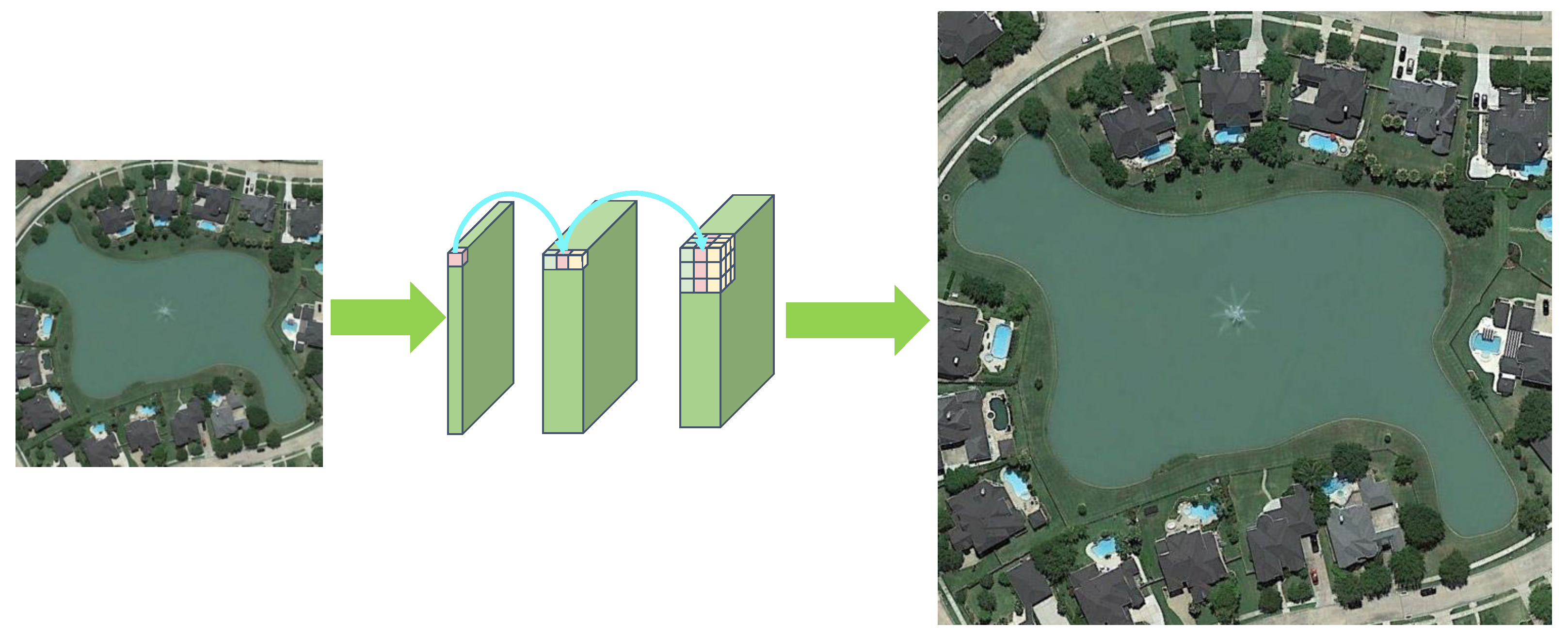
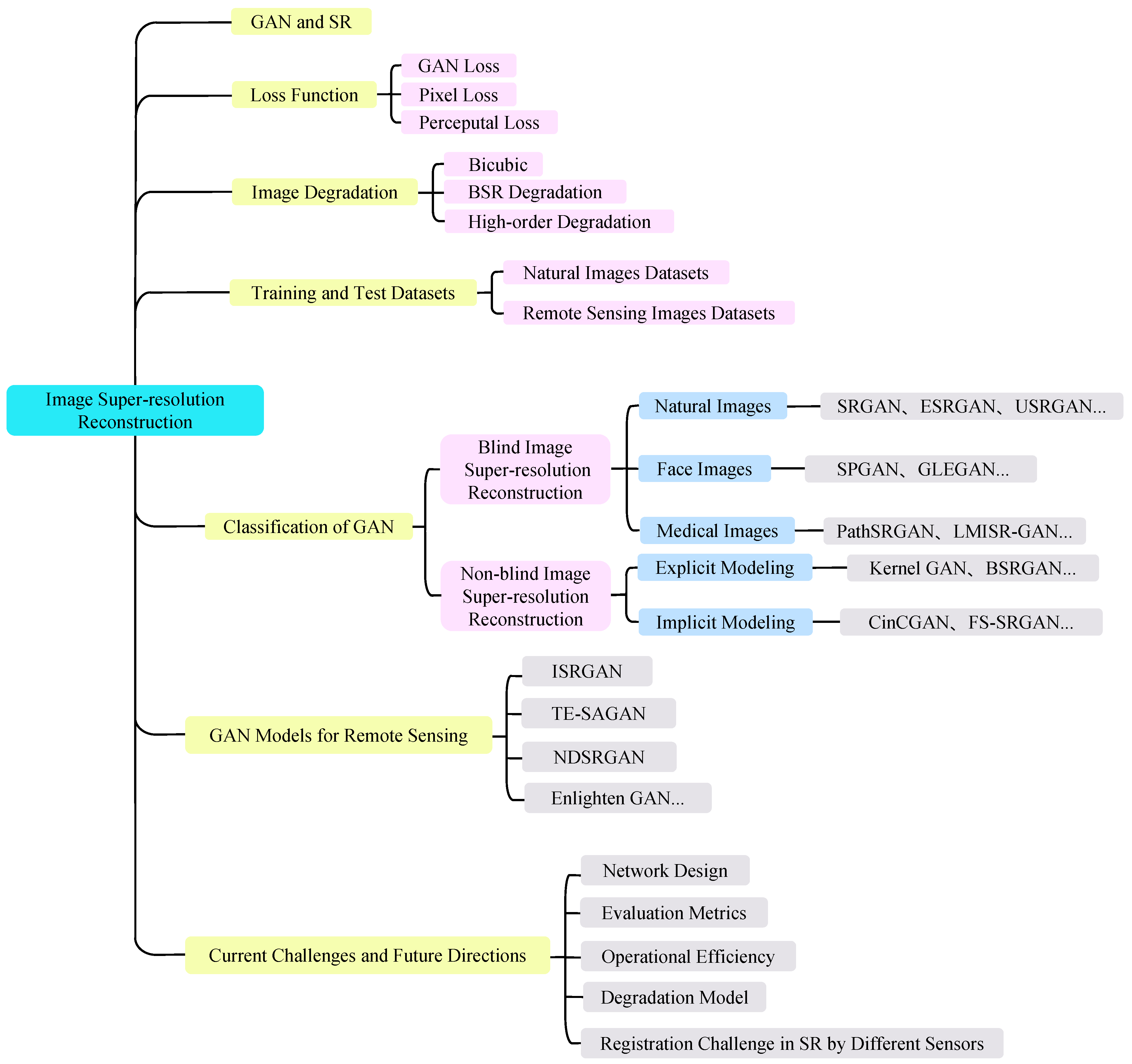
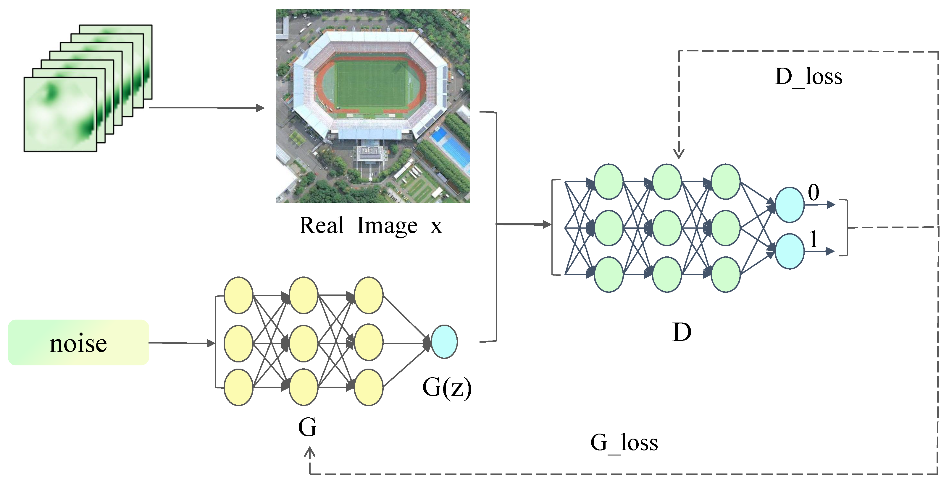
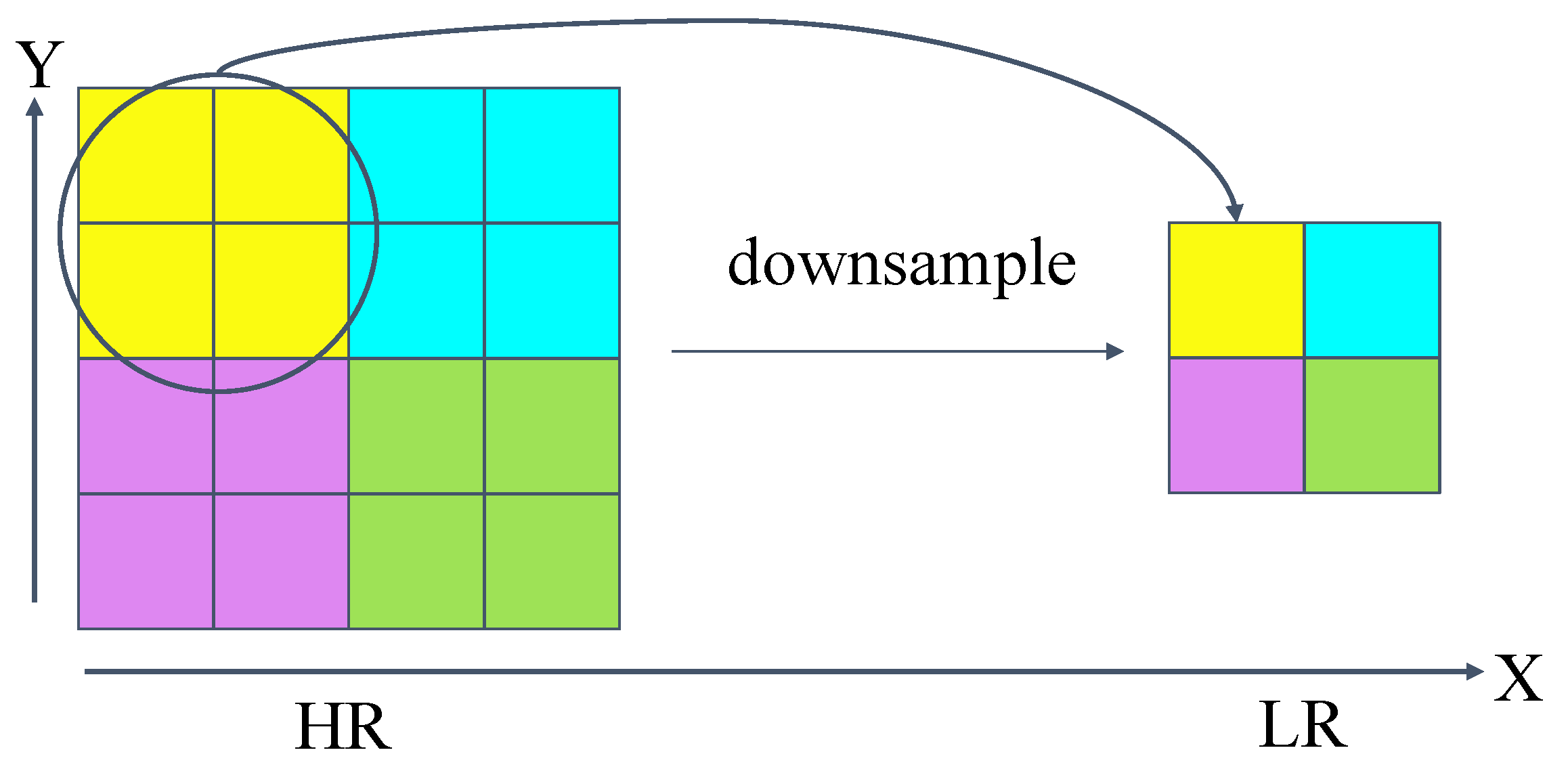
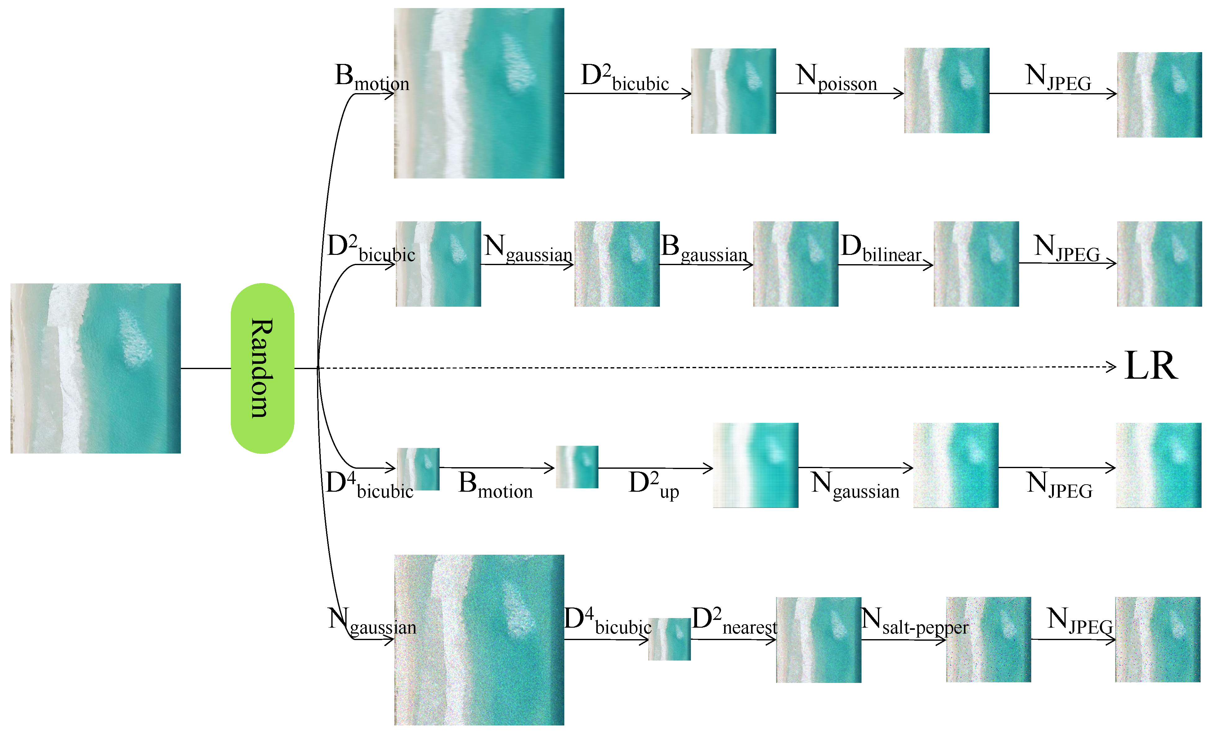
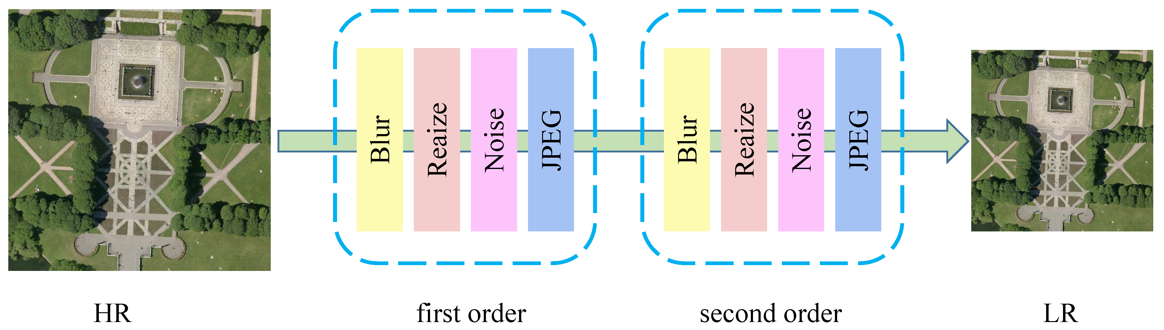
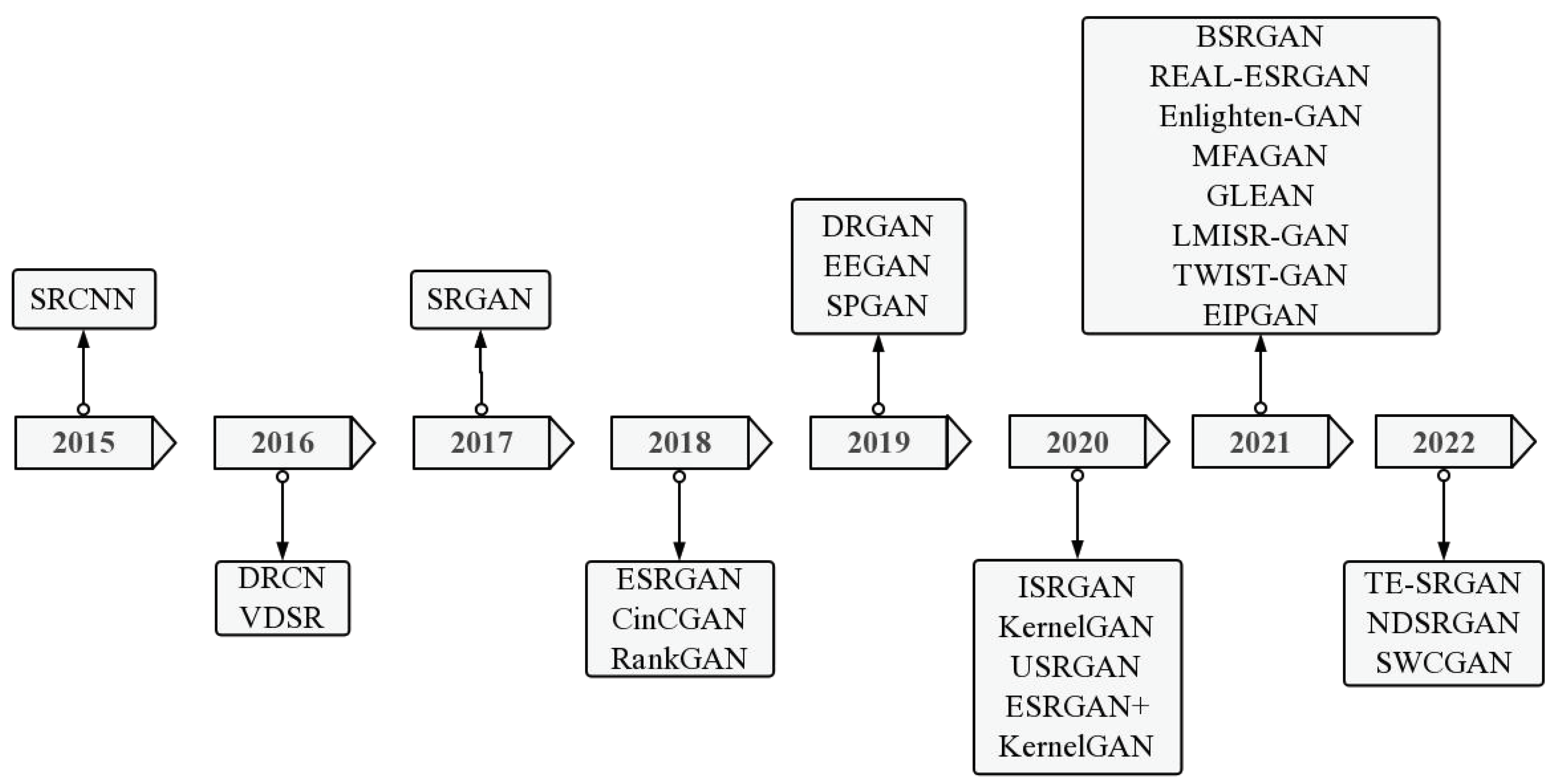
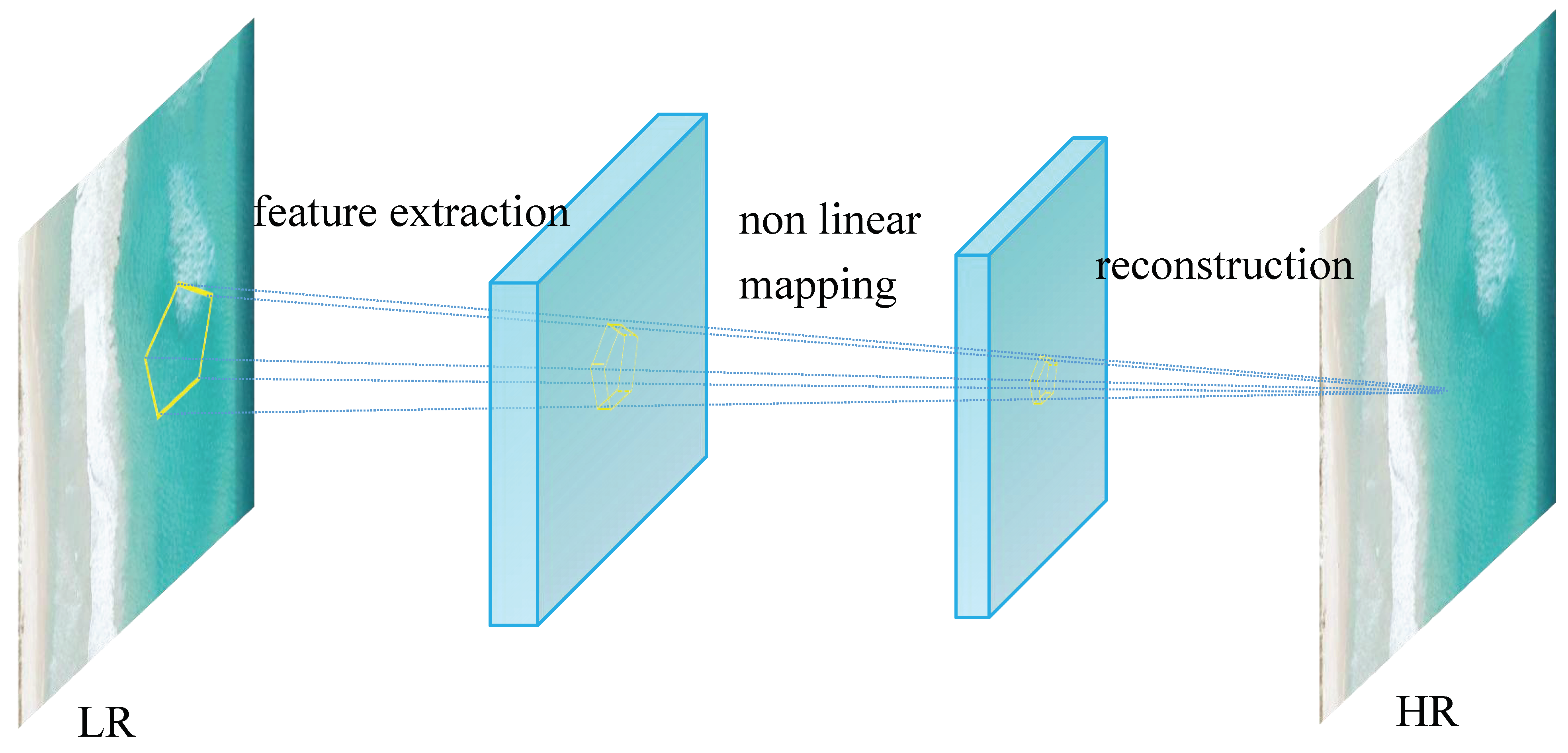
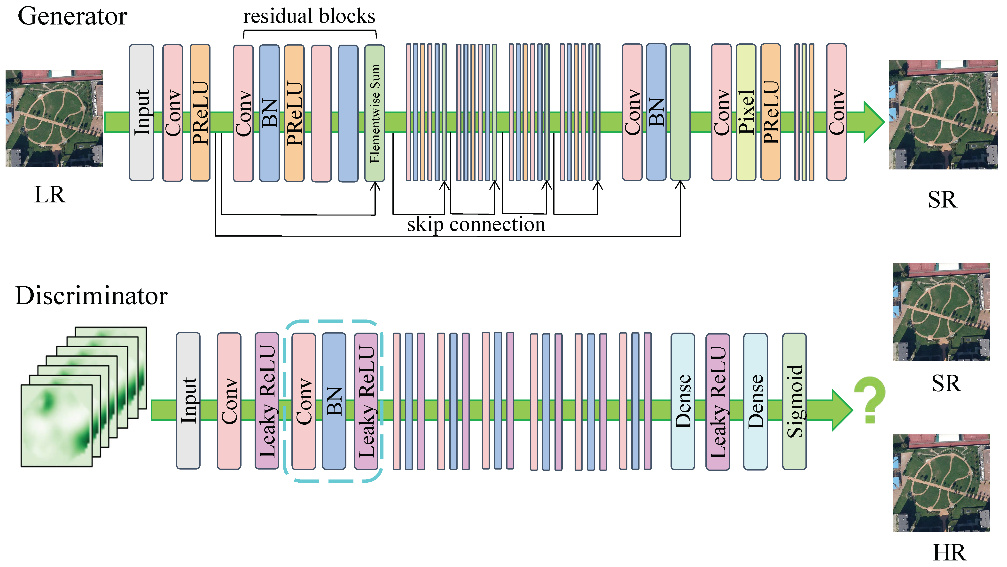
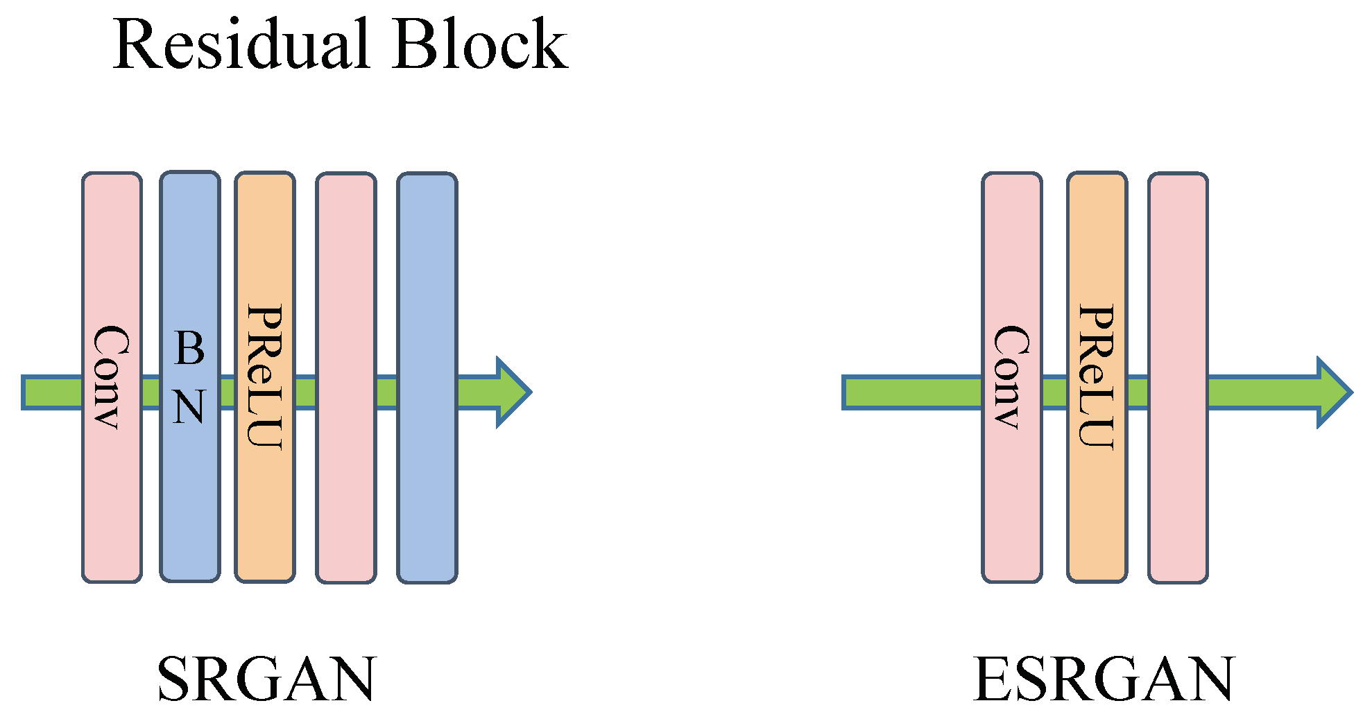
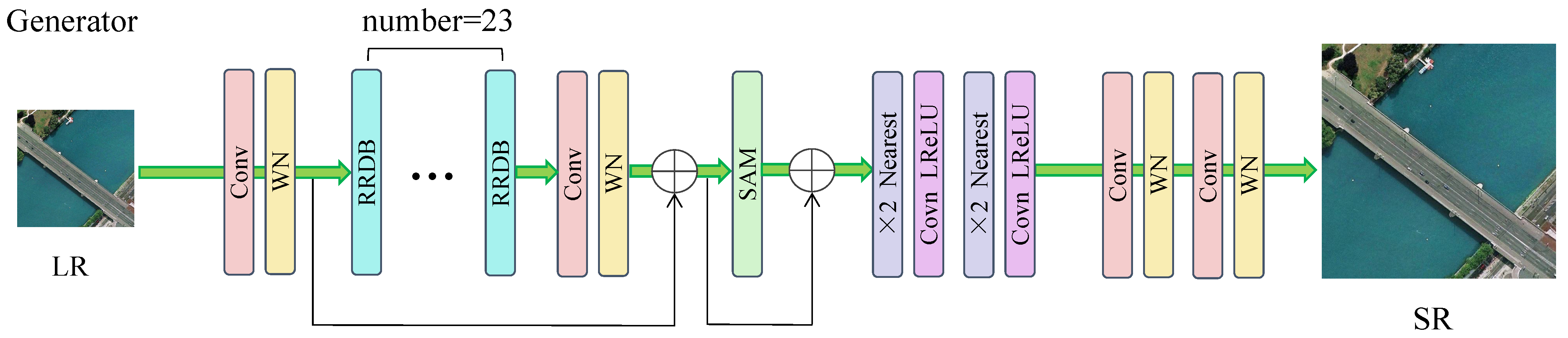
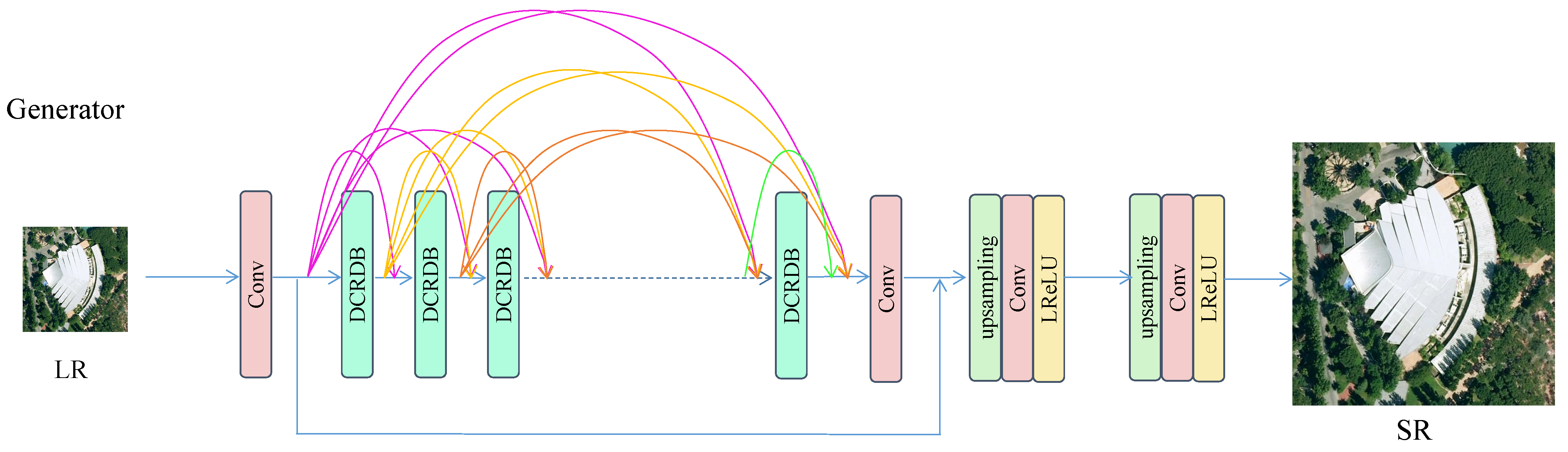
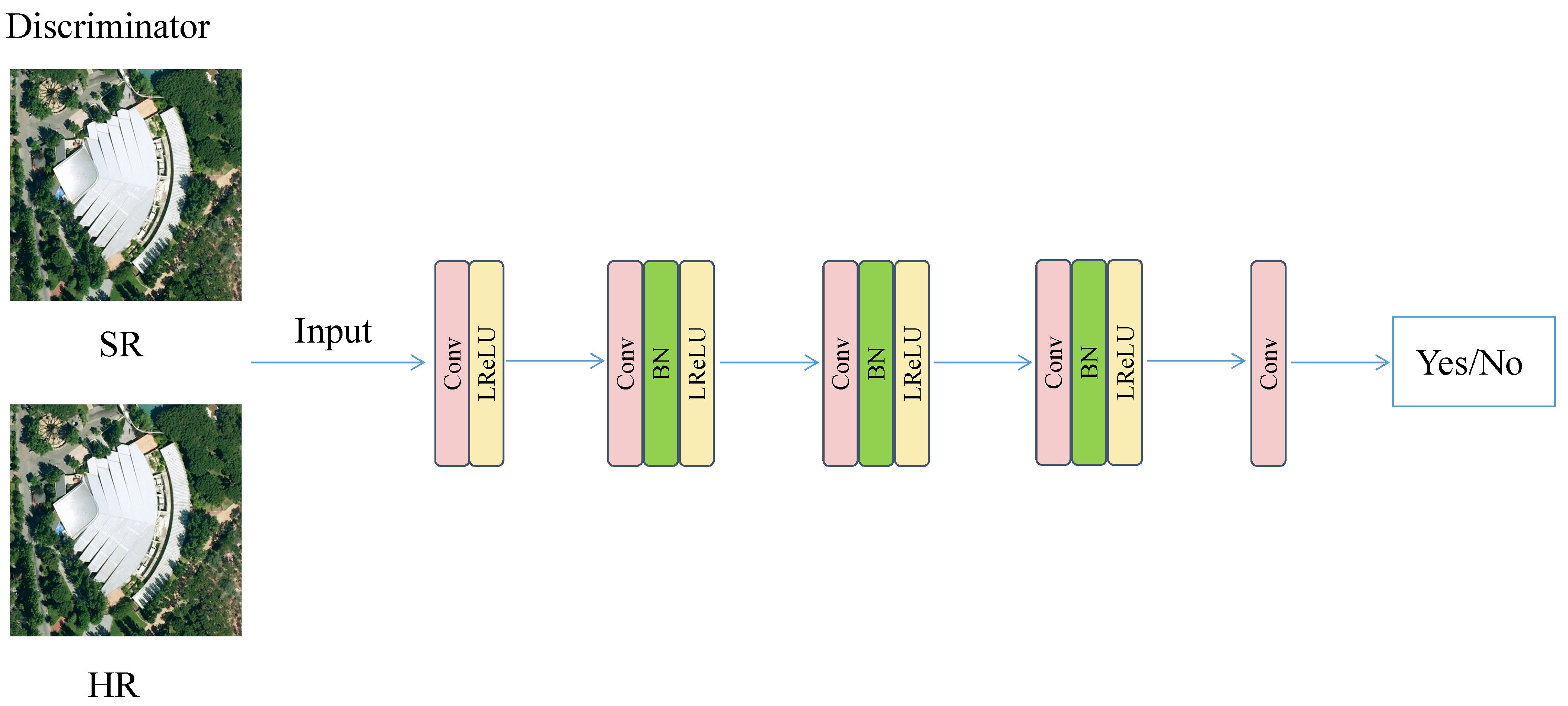
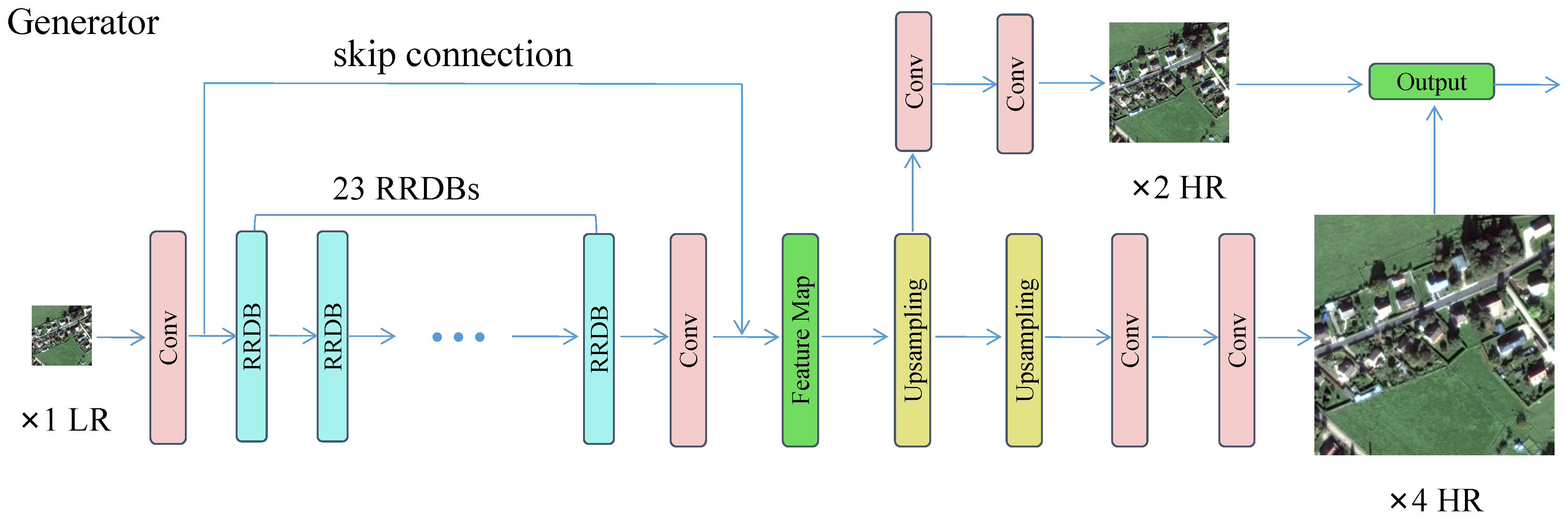
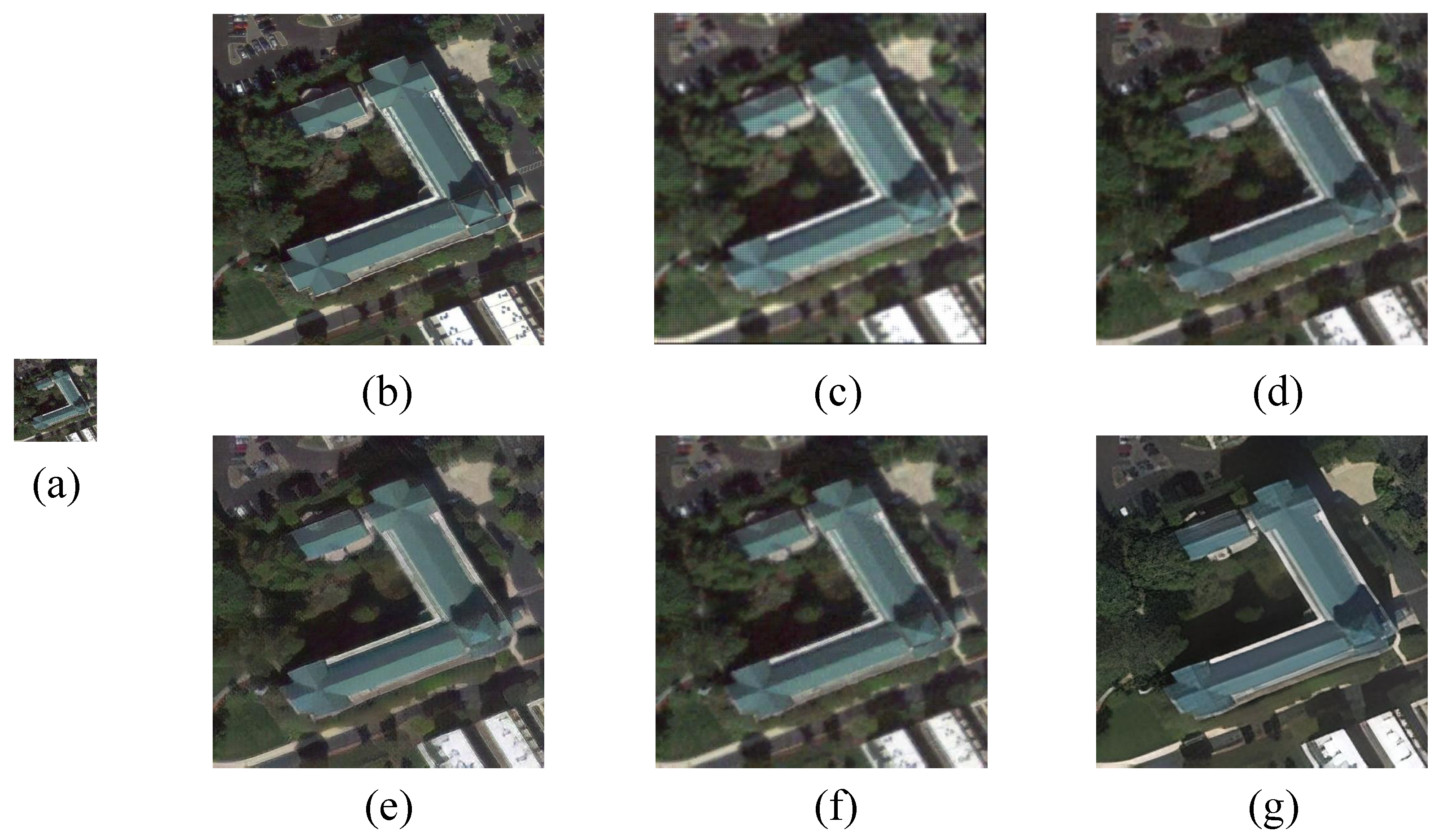
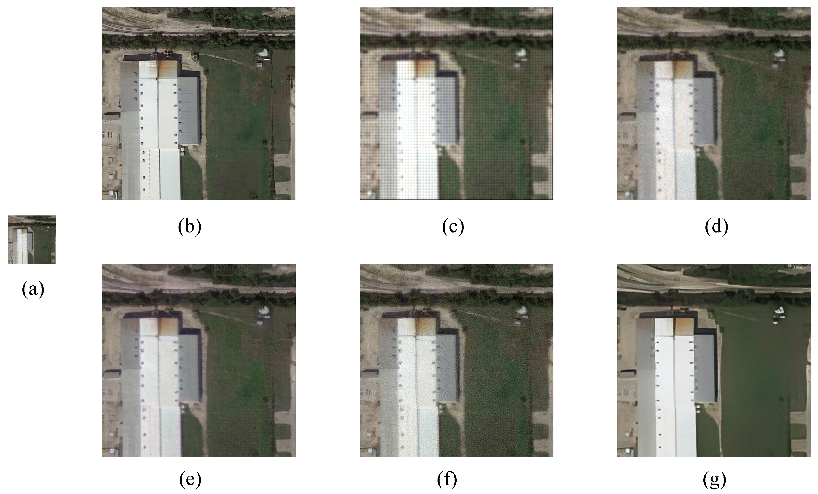
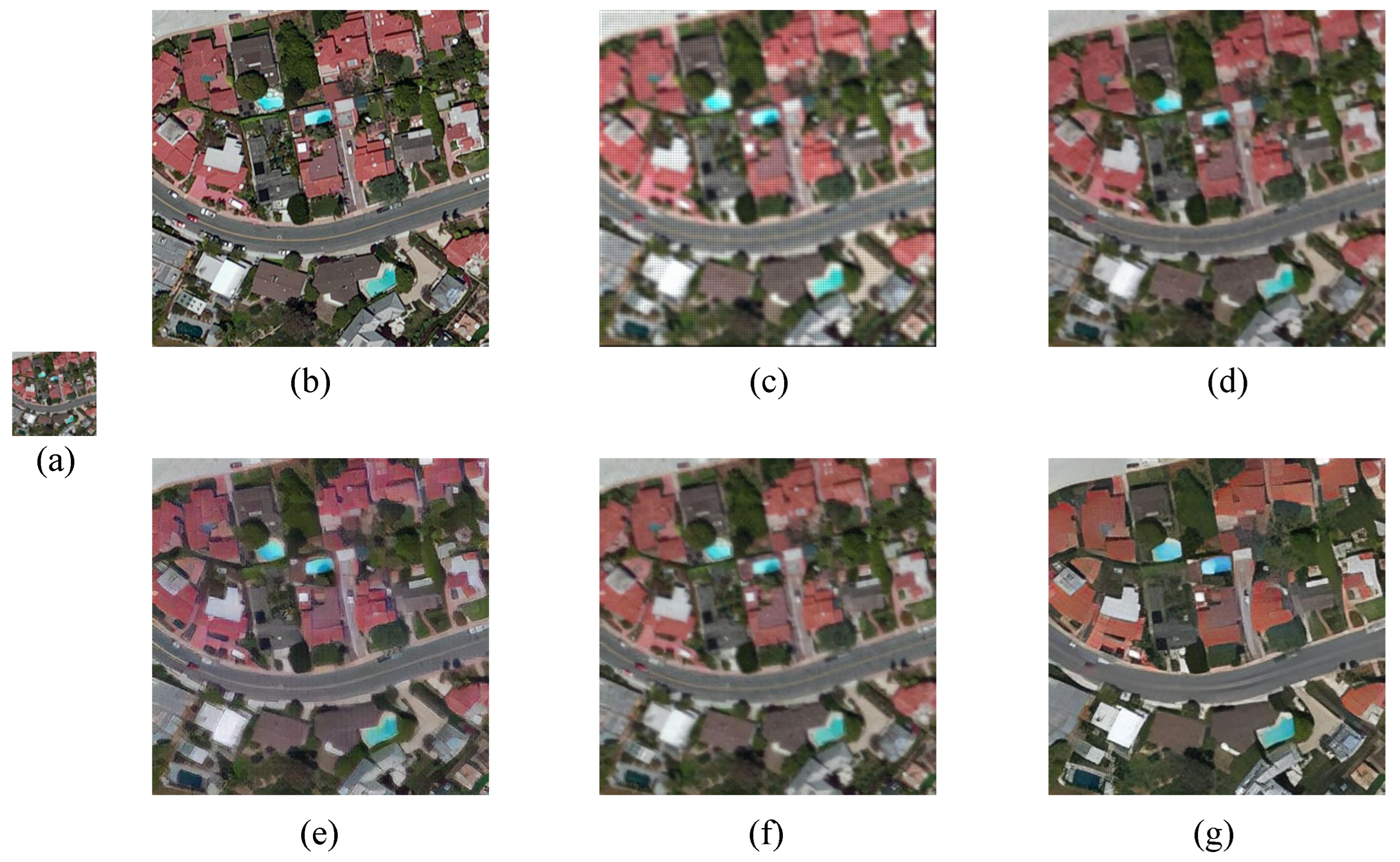
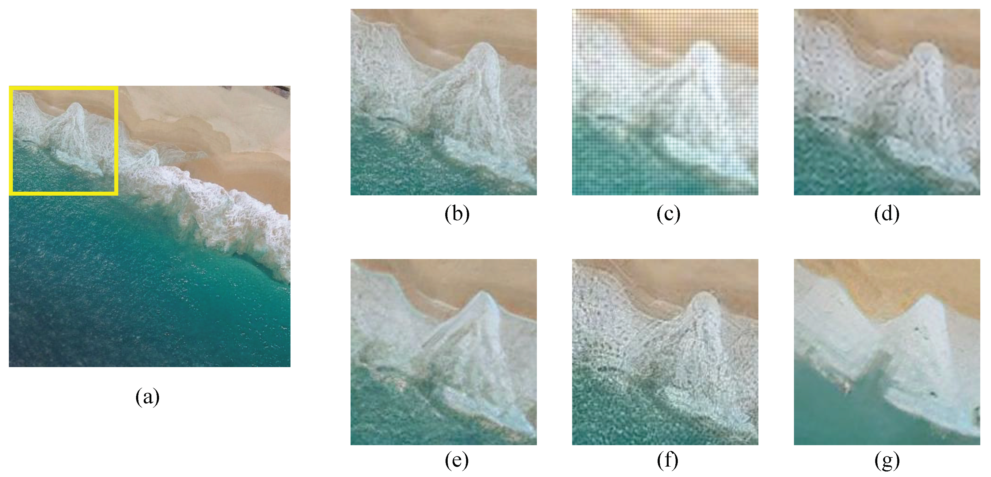
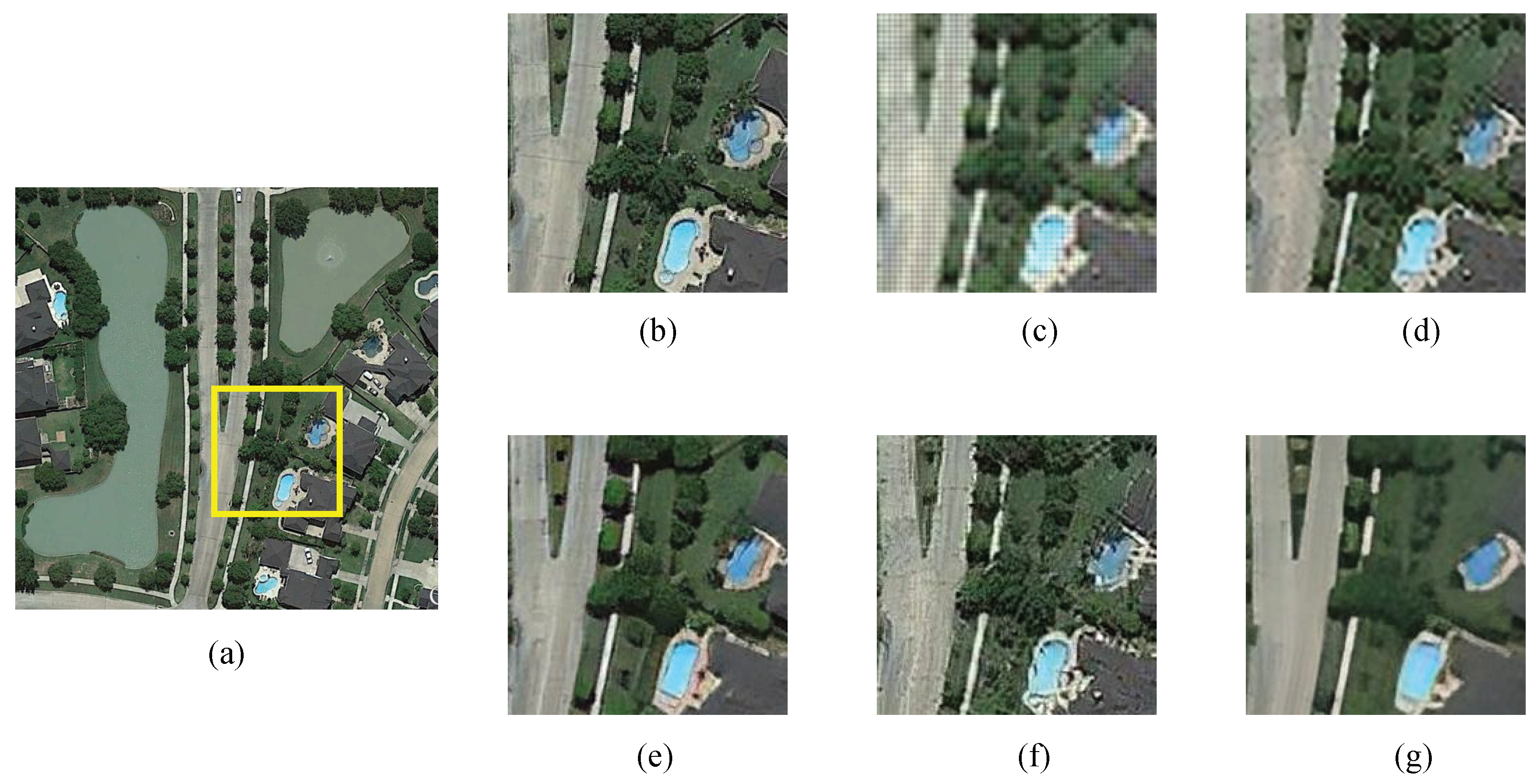
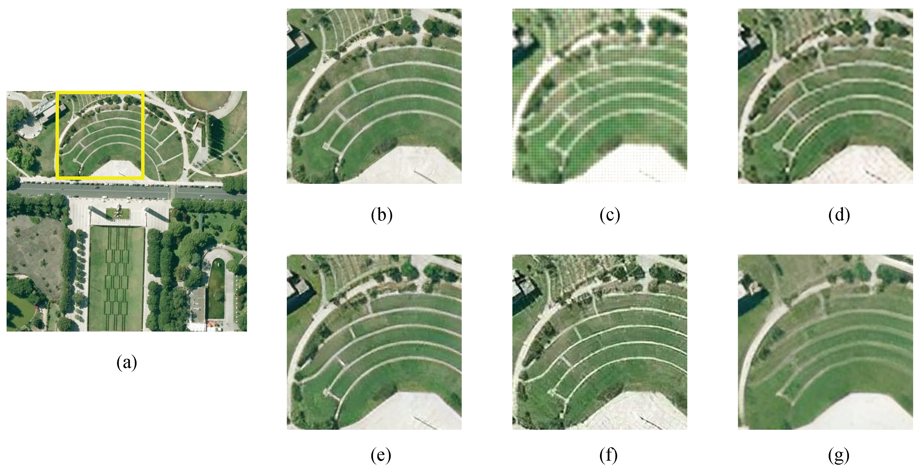
Table 1.
Commonly used natural and remotely sensed image datasets for super-resolution reconstruction tasks.
Table 1.
Commonly used natural and remotely sensed image datasets for super-resolution reconstruction tasks.
| Dataset | Format | Number | Resolution | Category |
|---|---|---|---|---|
| DIV2K [93] | PNG | 1000 | (1972, 1437) | people, scenery, animal, decoration, etc. |
| Flickr2K [94] | PNG | 2650 | (2048, 1080) | people, animal, flower, etc. |
| BSD300 [95] | JPG | 300 | (435, 367) | animal, scenery, decoration, plant, etc. |
| BSD500 [96] | JPG | 500 | (432, 370) | animal, scenery, decoration, plant, etc. |
| T91 [26] | PNG | 91 | (264, 204) | fruit, people, flower, etc. |
| Set5 [98] | PNG | 5 | (313, 336) | baby, butterfly, bird, head, woman |
| Set14 [99] | PNG | 14 | (492, 446) | pepper, zebra, coastguard, foreman, etc. |
| BSD100 [95] | JPG | 100 | (481, 321) | animal, scenery, plant, etc. |
| Urban100 [100] | PNG | 100 | (984, 797) | building, architecture, scenery, etc. |
| AID [102] | JPG | 10,000 | (600, 600) | airport, desert, farmland, pond, etc. |
| WHU-RS19 [103] | JPG | 1005 | (600, 600) | beach, bridge, forest, parking, etc. |
| UCAS-AOD [105] | PNG | 910 | (1280, 659) | car, airplane |
| RSC11 [106] | TIF | 1232 | (512, 512) | denseforest, grassland, roads, etc. |
| NWPU-RESISC45 [104] | PNG | 31,500 | (256, 256) | commercial area, harbor, island, etc. |
| RSSCN7 [107] | JPG | 2800 | (400, 400) | parking lots, residential areas, lakes, etc. |
| UC Merced [108] | PNG | 2100 | (256, 256) | farmland, bushes, highways, overpasses, etc. |
| SIRI-WHU [109] | TIF | 2400 | (200, 200) | agriculture, industrial, river, etc. |
| ITCVD [110] | JPG | 135 | (5616, 3744) | vehicles, buildings, etc. |
| DIOR [111] | JPG | 23,463 | (800, 800) | stadiums, bridges, dams, ports, etc. |
| DOTA [112] | PNG | 2806 | (800, 4000) | swimming pool, bridge, plane, ship, etc. |
Table 2.
Results of PNSR and SSIM for each model on each category of the RSC11 dataset.
| Bicubic PSNR/SSIM | SRGAN PSNR/SSIM | ESRGAN PSNR/SSIM | RankGAN PSNR/SSIM | BSRGAN PSNR/SSIM | |
|---|---|---|---|---|---|
| denseforest | 25.77/0.5288 | 26.66/0.5080 | 25.38/0.4106 | 24.73/0.3894 | 25.19/0.4398 |
| grassland | 24.22/0.4355 | 26.28/0.4577 | 26.05/0.4361 | 25.35/0.3971 | 27.57/0.5507 |
| harbor | 17.46/0.4169 | 18.76/0.4264 | 17.92/0.3649 | 17.89/0.3349 | 17.78/0.4094 |
| highbuildings | 19.52/0.4423 | 21.87/0.5612 | 20.62/0.4759 | 21.35/0.5056 | 20.68/0.5790 |
| lowbuildings | 18.72/0.3568 | 20.87/0.4777 | 20.11/0.4470 | 20.34/0.4177 | 20.07/0.4969 |
| overpass | 19.54/0.3797 | 21.43/0.4586 | 20.44/0.3893 | 20.39/0.3669 | 20.58/0.4502 |
| railway | 19.93/0.3703 | 22.45/0.4697 | 21.43/0.4186 | 21.51/0.3928 | 21.71/0.4905 |
| residentialarea | 19.76/0.4064 | 20.61/0.4398 | 19.96/0.3981 | 19.50/0.3514 | 19.55/0.4186 |
| roads | 19.94/0.4115 | 22.31/0.5031 | 21.25/0.4420 | 21.37/0.4325 | 21.12/0.4866 |
| sparseforest | 23.10/0.3627 | 24.67/0.3813 | 23.37/0.3041 | 23.60/0.3236 | 24.61/0.3806 |
| stroagetanks | 18.90/0.3764 | 20.62/0.4538 | 19.75/0.4053 | 19.96/0.3944 | 19.76/0.4629 |
Table 3.
Results of PNSR and SSIM for each model on each category of the AID dataset.
| Bicubic PSNR/SSIM | SRGAN PSNR/SSIM | ESRGAN PSNR/SSIM | RankSRGAN PSNR/SSIM | BSRGAN PSNR/SSIM | |
|---|---|---|---|---|---|
| Airport | 18.71/0.3662 | 26.27/0.7180 | 25.20/0.6576 | 25.14/0.6300 | 22.08/0.5507 |
| BareLand | 19.22/0.3204 | 32.18/0.8011 | 29.33/0.6849 | 31.48/0.7075 | 27.00/0.6718 |
| BaseballField | 20.92/0.4611 | 27.74/0.7553 | 26.27/0.6673 | 26.82/0.6721 | 23.51/0.6194 |
| Beach | 19.83/0.4054 | 29.54/0.7762 | 28.41/0.7258 | 29.38/0.7273 | 25.23/0.6835 |
| Bridge | 21.29/0.4974 | 28.35/0.7729 | 26.95/0.7192 | 27.14/0.7174 | 23.80/0.6497 |
| Center | 18.38/0.3911 | 24.51/0.6750 | 23.86/0.6310 | 23.74/0.6018 | 20.51/0.5095 |
| Church | 18.03/0.3816 | 21.88/0.5924 | 21.66/0.5557 | 21.19/0.5113 | 19.01/0.4103 |
| Commercial | 19/15/0.4390 | 25.36/0.6962 | 23.80/0.6023 | 23.58/0.5699 | 20.80/0.4654 |
| DenseResidential | 17.85/0.3779 | 22.24/0.6044 | 21.20/0.5189 | 21.17/0.5010 | 18.49/0.3568 |
| Desert | 18.52/0.2883 | 32.87/0.8360 | 31.89/0.7989 | 34.66/0.8186 | 30.47/0.8014 |
| Farmland | 21.98/0.4387 | 30.89/0.7701 | 29.47/0.7099 | 29.93/0.7037 | 26.92/0.6669 |
| Forest | 22.56/0.4284 | 26.56/0.6031 | 22.69/0.3757 | 24.41/0.4678 | 22.80/0.3242 |
| Industrial | 18.12/0.3761 | 24.70/0.6790 | 23.43/0.5999 | 23.32/0.5743 | 20.24/0.4531 |
| Meadow | 23.32/0.4351 | 30.56/0.6824 | 28.06/0.5241 | 28.50/0.5345 | 28.36/0.5984 |
| MediumResidential | 19.83/0.4032 | 24.86/0.6316 | 23.66/0.5457 | 23.99/0.5327 | 21.00/0.4270 |
| Mountain | 20.82/0.4369 | 27.01/0.6874 | 24.40/0.4992 | 24.85/0.5176 | 22.16/0.4137 |
| Park | 20.07/0.4404 | 26.03/0.6894 | 24.06/0.5691 | 24.22/0.5508 | 21.73/0.4647 |
| Parking | 17.25/0.3817 | 22.67/0.7014 | 21.93/0.6512 | 21.96/0.6079 | 18.35/0.4941 |
| Playground | 20.36/0.4458 | 27.97/0.7531 | 26.39/0.6833 | 27.22/0.6921 | 23.27/0.6163 |
| Pond | 21.80/0.4966 | 27.79/0.7419 | 26.22/0.6679 | 26.64/0.6734 | 24.13/0.6180 |
| Port | 19.06/0.4847 | 24.64/0.7510 | 23.71/0.7195 | 23.60/0.6937 | 20.60/0.6256 |
| RailwayStation | 18.99/0.3883 | 25.72/0.6822 | 24.29/0.5935 | 24.22/0.5732 | 21.17/0.4388 |
| Resort | 18.91/0.4112 | 25.38/0.6890 | 23.74/0.5930 | 24.18/0.5872 | 20.98/0.4875 |
| River | 21.64/0.4448 | 28.26/0.7058 | 25.94/0.5785 | 26.57/0.5881 | 24.38/0.5355 |
| School | 19.06/0.4367 | 24.58/0.6774 | 23.06/0.5773 | 23.27/0.5669 | 20.18/0.4503 |
| SparseResidential | 21.27/0.3773 | 24.71/0.5649 | 22.95/0.4223 | 23.24/0.4302 | 21.73/0.3343 |
| Square | 18.90/0.4124 | 26.08/0.7068 | 24.59/0.6290 | 25.08/0.6186 | 21.17/0.5121 |
| Stadium | 18.69/0.4245 | 24.97/0.7011 | 24.19/0.6520 | 24.15/0.6320 | 20.70/0.5352 |
| StorageTanks | 18.71/0.3871 | 24.20/0.6511 | 23.49/0.5915 | 23.30/0.5620 | 20.55/0.4821 |
| Viaduct | 19.57/0.4066 | 25.47/0.6656 | 24.13/0.5750 | 24.17/0.562 | 21.24/0.4380 |
Disclaimer/Publisher’s Note: The statements, opinions and data contained in all publications are solely those of the individual author(s) and contributor(s) and not of MDPI and/or the editor(s). MDPI and/or the editor(s) disclaim responsibility for any injury to people or property resulting from any ideas, methods, instructions or products referred to in the content. |
© 2023 by the authors. Licensee MDPI, Basel, Switzerland. This article is an open access article distributed under the terms and conditions of the Creative Commons Attribution (CC BY) license (https://creativecommons.org/licenses/by/4.0/).
Share and Cite
MDPI and ACS Style
Wang, X.; Sun, L.; Chehri, A.; Song, Y. A Review of GAN-Based Super-Resolution Reconstruction for Optical Remote Sensing Images. Remote Sens. 2023, 15, 5062. https://doi.org/10.3390/rs15205062
AMA Style
Wang X, Sun L, Chehri A, Song Y. A Review of GAN-Based Super-Resolution Reconstruction for Optical Remote Sensing Images. Remote Sensing. 2023; 15(20):5062. https://doi.org/10.3390/rs15205062
Chicago/Turabian StyleWang, Xuan, Lijun Sun, Abdellah Chehri, and Yongchao Song. 2023. "A Review of GAN-Based Super-Resolution Reconstruction for Optical Remote Sensing Images" Remote Sensing 15, no. 20: 5062. https://doi.org/10.3390/rs15205062
Note that from the first issue of 2016, this journal uses article numbers instead of page numbers. See further details here.