
Single-Image Super Resolution of Remote Sensing Images with Real-World Degradation Modeling


1
School of Optics and Photonics, Beijing Institute of Technology, Beijing 100081, China
2
Beijing Institute of Technology Chongqing Innovation Center, Chongqing 401120, China
*
Author to whom correspondence should be addressed.
Remote Sens. 2022, 14(12), 2895; https://doi.org/10.3390/rs14122895
Submission received: 25 April 2022
/
Revised: 10 June 2022
/
Accepted: 13 June 2022
/
Published: 17 June 2022
(This article belongs to the Special Issue Advanced Super-resolution Methods in Remote Sensing)
Abstract
:Limited resolution is one of the most important factors hindering the application of remote sensing images (RSIs). Single-image super resolution (SISR) is a technique to improve the spatial resolution of digital images and has attracted the attention of many researchers. In recent years, with the advancement of deep learning (DL) frameworks, many DL-based SISR models have been proposed and achieved state-of-the-art performance; however, most SISR models for RSIs use the bicubic downsampler to construct low-resolution (LR) and high-resolution (HR) training pairs. Considering that the quality of the actual RSIs depends on a variety of factors, such as illumination, atmosphere, imaging sensor responses, and signal processing, training on “ideal” datasets results in a dramatic drop in model performance on real RSIs. To address this issue, we propose to build a more realistic training dataset by modeling the degradation with blur kernels and imaging noises. We also design a novel residual balanced attention network (RBAN) as a generator to estimate super-resolution results from the LR inputs. To encourage RBAN to generate more realistic textures, we apply a UNet-shape discriminator for adversarial training. Both referenced evaluations on synthetic data and non-referenced evaluations on actual images were carried out. Experimental results validate the effectiveness of the proposed framework, and our model exhibits state-of-the-art performance in quantitative evaluation and visual quality. We believe that the proposed framework can facilitate super-resolution techniques from research to practical applications in RSIs processing.
1. Introduction
Remote sensing images (RSIs) captured using satellites or aircraft are essential in many applications such as environmental surveys [1,2], disaster monitoring [3,4], and resource censuses [5,6]. Spatial resolution is one of the most important metrics of RSIs that advanced satellites or aircraft researchers have been striving to improve; however, the high cost of high-performance imaging systems and harsh imaging conditions in space limit the resolution of RSIs to sub-meter levels. Single image super resolution (SISR) is a technique for reconstructing high-resolution (HR) images from low-resolution (LR) observations [7,8,9]. It is widely employed in a range of scenarios such as mobile devices, medical imaging, and remote sensing. It has been a research hotspot in the field of low-level image processing for decades.
SISR is an ill-posed problem since high-frequency information is lost during imaging. A single LR image may correspond to multiple HR solutions [7,10,11]. To address this problem, many practical frameworks have been proposed, which can be grouped into three categories: (i) interpolation-based methods, (ii) reconstruction-based methods, and (iii) learning-based methods.
Interpolation-based methods estimate missing pixel values with different interpolation functions such as bilinear, bicubic, and spline [12]. These methods are commonly used to scale images due to their high computational efficiency but often lead to over-smoothed results. Reconstruction-based methods attempt to investigate image degradation processes, such as out-of-focus, motion, aliasing, and noise, and build models to implement the inverse process. Reconstruction-based methods can recover sharp details with prior information of the degradation process, but suffer from heavy computation and reconstruction artifacts. Learning-based approaches learn the mapping between LR and HR images in the collected dataset and try to generalize to images outside the dataset. In recent years, convolutional neural networks (CNN) have received increasing attention due to their excellent nonlinear representation and feature extraction capabilities. Many CNN-based methods are proposed to solve the SISR problem and achieve state-of-the-art performance. Lu [13] proposed a multi-scale residual neural network (MRNN), which adopts the multi-scale properties to reconstruct high-frequency information accurately for the super resolution (SR) of RSIs. Xiong [14] modified the loss function and the structure of the super-resolution generative adversarial network (SRGAN) for SR of RSIs.
Deep learning (DL) methods have achieved promising results on SR of RSIs, but there are still some problems. Current datasets for the SR of RSIs, such as AID [15], UCMERCED [16], and RSIs-CB256 [17], are not designed for real-world situations. Since the HR observations for RSIs datasets are difficult to obtain, most RSIs datasets actually contain only LR images. To build input–target pairs to train the deep neural network, most studies [18,19,20] employ a simple strategy of generating lower resolution (abbreviated as LR’) images from LR images with bicubic interpolation. Networks trained on LR’–LR pairs can achieve satisfactory results on the test dataset since the test images are also LR’ images instead of the actual RSIs; however, the LR’–LR mapping is quite different from the LR–HR mapping. Due to the imperfect illumination, atmospheric propagation, lens imaging, sensor quantification, etc., the RSIs suffers from image degradation such as blur and noise. In addition, the image degradation can be mitigated through downsampling; therefore, the learned mapping comes from clean LR’ images to contaminated LR images instead of the expected mapping from contaminated LR images to clean HR images. This is the main reason why many previous studies can achieve excellent experimental results, but face performance degradation in practical scenarios.
To address this issue, inspired by recent advanced research [21,22,23], we apply a framework to construct realistic datasets by modeling real-world degradation in remote sensing images. As the realistic SISR task is more complicated than the ideal SISR task, we also propose a novel neural network with a balanced attention mechanism to achieve better performance. More specifically, we classify the degradation of RSIs into two categories, blur and noise. The blur simulates the diffraction limit of a lens, the disturbance of atmosphere, and the relative movement of image platforms to the Earth. The noise includes different kinds of imaging noise and JPEG compression noise. Blur kernels and noise patterns are collected and randomly used to synthesize realistic LR images and construct LR–HR training pairs. By training on realistic datasets, the performance of the model under real-world conditions can be significantly improved. As for the network, we propose a residual balanced attention network (RBAN) that integrates the residual in the residual structure and a balanced attention mechanism. A modified UNet model is adopted as a pixel-wise discriminator to achieve more realistic SISR results. Thorough experiments were conducted and the results demonstrate the effectiveness of the proposed framework and neural network.
The contributions of this study are highlighted as follows: (i) We propose a framework integrating blur kernel estimation and noise pattern extraction to model the degradation of remote sensing images; (ii) we construct a realistic RSIs dataset based on the open source Aerial Image Dataset (AID) for training and testing, which greatly enhances the performance of models on real RSIs; (iii) we propose a novel SISR model termed residual balanced attention network (RBAN) and apply a modified UNet model as the discriminator to improve perceptual performance. The proposed model achieves state-of-the-art performance on the realistic RSIs dataset.
The rest of this paper is organized as follows. In Section 2, related works about CNN-based SISR methods and RSIs SISR methods are summarized. In Section 3, the framework and model are proposed. Section 4 details the experimental results of the proposed method and compares it with the state-of-the-art methods. Conclusions are drawn in Section 5.
2. Releated Work
2.1. CNN-Based SISR Methods
Since the advent of CNN, it has outperformed traditional methods in a growing number of computer vision tasks, including SISR. To solve the SISR problem with CNN, Dong et al. [24] proposed a shallow super-resolution CNN (SRCNN), which can learn the mapping from interpolated LR images to HR images. SRCNN outperforms state-of-the-art traditional SISR methods such as K-SVD [25] and ANR [26], and attracts more researchers to study the CNN-based SISR methods. Later, Caballero et al. [27] proposed to use the pixel-shuffle layer to improve the spatial resolution of feature maps so that computations could be performed in LR space to reduce the computational effort. SRCNN contains only three convolutional layers, which limits its performance. To deepen the network and obtain stronger learning ability, Kim et al. [28] applied the residual learning strategy and proposed a 20-layer very deep super resolution (VDSR) model. Due to its larger receptive field, the reconstruction performance of VDSR is much better than that of SRCNN, and the residual learning strategy has become the standard configuration for CNN-based SISR since then. Inspired by VDSR, Ledig et al. [29] proposed SRResNet, which employs the residual learning strategy both globally and locally. Ledig also proposed the generative adversarial training framework SRGAN, which enables photo-realistic SISR. Since SRGAN, GAN-based methods have become the dominant framework for better perceptual results. By removing the batch normalization layer in SRResNet, Lim et al. [30] proposed an optimized residual block module and an enhanced deep super-resolution network (EDSR). Inspired by the channel attention mechanisms commonly used in high-level computer vision problems such as classification and detection, Zhang et al. [31] proposed a deep residual channel attention network (RCAN). Subsequently, Liang et al. [23] successfully adopted the shifted windows transformer module in SISR and proposed a state-of-the-art model SwinIR. Anwar [32] proposed a densely residual Laplacian network (DRLN), which employs cascading residual structure to allow low-frequency information flow to focus on learning high and mid-level features.
Nowadays, SISR has become one of the most important tasks in many computer vision challenges such as NTIRE [9] and AIM [8]. With the practical application of super-resolution technology, researchers began to realize the limitations of previous studies. The common practice for building super-resolution training datasets is to collect a large number of HR images and downsample them using bicubic interpolation; however, in real-world imaging, bicubic interpolation is insufficient to describe the degradation process; therefore, the focus of SISR research in recent years has gradually shifted to real-world SISR that takes into account degradations such as blur and noise. One of the representative strategies is to directly collect and align LR–HR pairs. Zhang et al. [33] captured images with a zoomable lens in different magnifications and carefully aligned the LR and HR images spatially. Trained on real-world LR–HR pairs, Zhang’s network achieved much better results on real-world images than networks trained on synthetic datasets. An alternative strategy is to model the degradation process and try to synthesize more realistic LR observations from HR images. Bell-Kligler et al. [21] proposed to use blur kernels to model the degradation and GANs to estimate the kernels. Another strategy is to train the network with unpaired real-world LR and HR images. Yuan et al. [34] proposed a cycle-in-cycle GAN, which treats the SISR as a domain translation task from LR space to HR space.
2.2. SISR of RSIs
Due to the huge demand for high spatial resolution in many remote sensing tasks such as scene classification, object detection, and instance segmentation, SISR has become a research hotspot in RSIs processing. Nguyen and Milanfar [35] first decomposed LR images with discrete wavelet transform (DWT), then used an interpolation algorithm to upsample the wavelet coefficients, and finally inverse transformed the coefficients to generate HR images. Based on maximum posterior probability, Li et al. [36] proposed a generalized hidden Markov tree model (MAP-uHMT) that uses a hybrid Gaussian model to represent the wavelet coefficients of an image and a hidden Markov tree to capture the dependencies between multiscale wavelet coefficients. Pan et al. [37] proposed a dictionary learning method for SISR of RSIs that combines compressed sensing and structural self-similarity.
In recent years, CNN-based methods have become the mainstream of SISR for RSIs due to their outstanding performance and extensive applicability. Lei et al. [38] proposed a SISR model named local–global combined networks (LGCNet) for RSIs based on CNN. LGCNet applied a novel ‘multifork’ structure to learn multilevel representations of RSIs including local details and global environmental priors. Jiang et al. [39] proposed a deep distillation recursive network (DDRN) effective for video satellite image SR. DDRN uses dense connections to create more linked nodes and a distillation compensation mechanism to compensate for high-frequency information to reconstruct more accurate SR images. Ma et al. [40] proposed a method that incorporates DWT to decompose LR images and recursive ResNet to predict high-frequency components; then, the reconstructed HR image can be obtained via inverse DWT. Zhang et al. [18] proposed a multiscale attention network (MSAN) to extract the multilevel features of RSIs. A scene-adaptive super-resolution strategy was also applied to more accurately describe the structural features of different scenes in MSAN. Guo et al. [41] designed a novel dense generative adversarial network (NDSRGAN) that integrates a multilevel dense network and a matrix mean discriminator for aerial imagery SR reconstruction.
3. Methodology
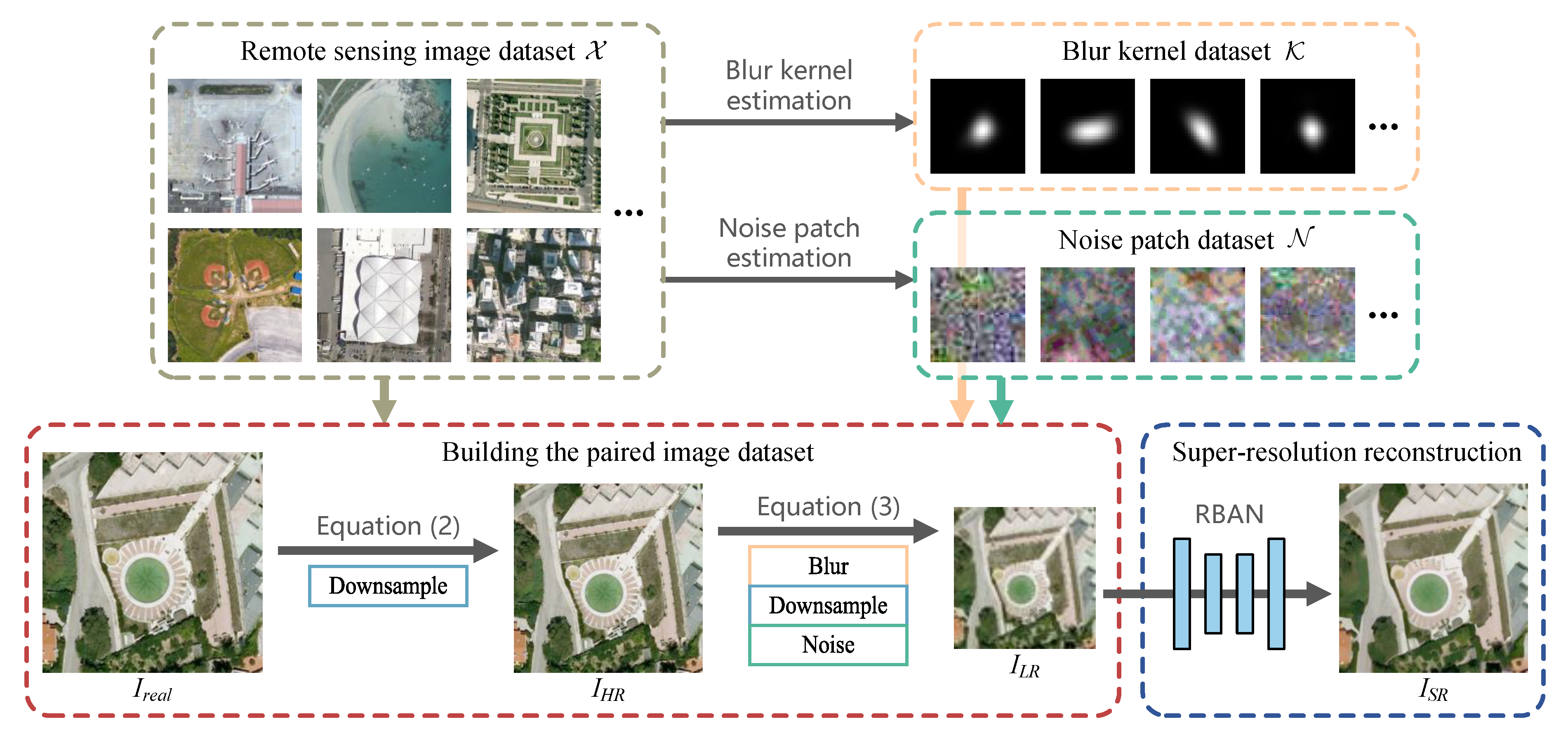
In this section, we introduce the proposed framework as shown in Figure 1. The framework is mainly divided into three stages. The first is to estimate blur kernels and noise patches from the real RSIs dataset, which is detailed in Section 3.2. The second is to generate a realistic synthetic training dataset with the real RSIs dataset and collected blur kernels and noise patches, which is detailed in Section 3.1. The third is to train a novel network based on the synthetic dataset, which is detailed in Section 3.3.
3.1. Realistic Degradation for SISR of RSIs
Previous SISR methods of RSIs model the imaging process as follows
where and denote the LR and HR remote sensing images, respectively, and s denotes the downsample scale factor. This makes it easy to generate LR images from real RSIs and train a network for reverse mapping; however, the model in Equation (1) is too simplistic and distorts the actual degradation process of RSIs. RSIs in real-world conditions contain blur and noise due to the imperfect illumination, atmospheric propagation, lens imaging, sensor quantification, In addition, the downsampling process can suppress blur and high-frequency noise; therefore, the network based on Equation (1) will learn a mapping from clean LR images to realistic HR images, which is inconsistent with the desired mapping from realistic LR images to clean HR images. This is why previous methods suffer from performance degradation when dealing with real-world RSIs.
To settle the aforementioned problem, we proposed to construct a realistic training dataset for SISR of RSIs using the following degradation model
where and represent the blur kernel and noise, respectively. indicates the real RSIs in the dataset, indicates the clean HR image generated by downsampling the real RSIs and indicates the synthetic realistic LR image. c and s are the downsampling scales of HR and LR images, respectively. The blur kernel and noise are collected from the dataset of real RSIs, so a more realistic dataset can be constructed by randomly combining the blur kernels, noise patches, and real RSIs. With the realistic dataset, a more robust CNN can be trained. The whole pipeline of constructing paired LR–HR images with real RSIs is shown in Algorithm 1.
| Algorithm 1 Realistic data pairs generation |
|
(1) Blur: Blur is a common degradation during the imaging of RSIs. We model the blur of RSI as a convolution with a blur kernel (filter). In earlier research, the blur kernel of a LR image was usually assumed to be the point spread function (PSF) of the camera; however, blur can be caused by a variety of reasons such as limited lens aperture, defocus, relative motions between image platforms, and the Earth. Thus, the blur kernel of a known imaging system may vary under different circumstances. It has been proved by Michaeli [42] that the correct SR blur kernels can be recovered directly from low-resolution images.
(2) Noise: Noise is another common degradation that can be divided into two main categories, imaging noise and processing artifacts. Imaging noises are caused by undesired responses of sensor during image capture. Imaging noises caused by different factors satisfy different statistical distributions, such as Gaussian distribution and Poisson distribution. Due to the limited download bandwidth of satellites or airplanes, RSIs is usually compressed with JPEG algorithm; however, the JPEG compression results in loss of high-frequency information and introduces undesired artifacts.
3.2. Estimation of Blur Kernel and Noise Patches
In this section, we detail the methods for estimating blur kernels and noise patches.
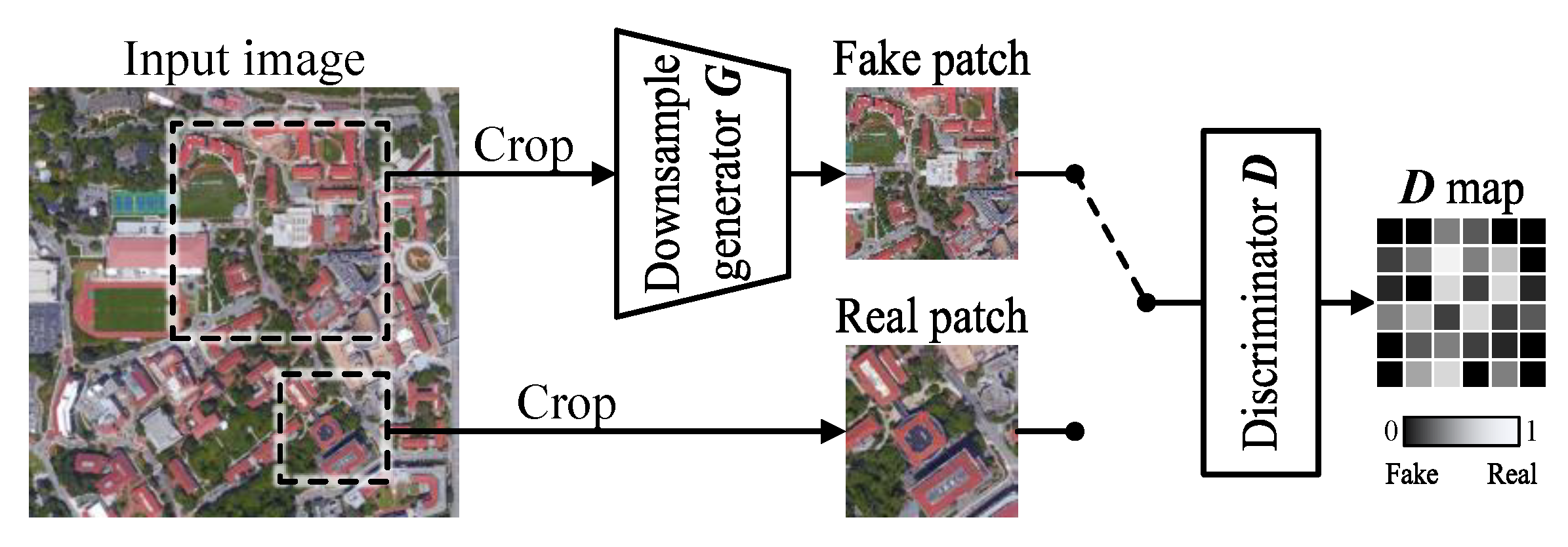
(1) Blur kernel estimation: There are mainly two strategies to build the blur kernel dataset. One is to model kernels with isotropic or anisotropic Gaussian distributions and generate kernels with random parameters within a preset range. Another strategy is to estimate and collect kernels from real images. We adopt the second strategy and apply a modified version of KernelGAN [21] presented by Ji et al. [22]. The authors hypothesized that the correct SR kernel maximizes the recurrence of patches between LR and HR images. As shown in Figure 2, KernelGAN is composed of a generator G and a discriminator D. G is a five-layer full convolutional neural network and is trained to produce downsampled patches of the input image. D is trained to distinguish downsampled image patches from original image patches. Then, the kernel can be explicitly extracted by convolving all the layers of G sequentially with stride 1.
The KernelGAN is designed to solve the following problem
The first term in the above equation encourages the downsampled image to preserve important low-frequency information of the source image. The second term constrains to sum to 1 and the third term penalizes non-zero values near the boundaries with a constant mask. At last, the discriminator ensures the consistency of source domain.
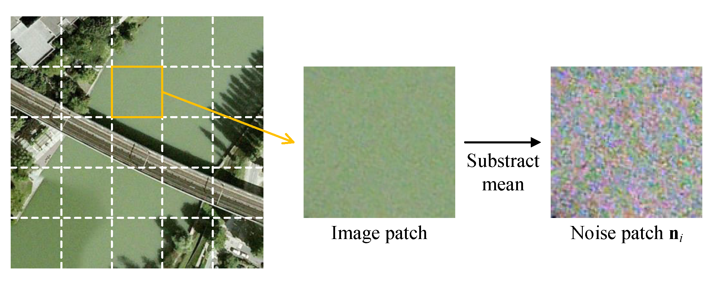
(2) Noise estimation: Since the noise in the image is a mixture of a series of noise sources, such as thermal noise, read noise, signal disturbance, and JPEG compression. It is difficult to accurately calibrate the type and weight of each noise source; however, we find that image variances in flat scene regions, such as water surface or bare land, are mainly caused by noise. Based on this assumption, we can decouple noise and content by using a simple but effective rule:
where denotes to calculate variance, v is the threshold of variance, and is the image patch after subtracting the mean. The process of collecting noise patches is shown in Figure 3.
3.3. Residual Balanced Attention Network (RBAN)
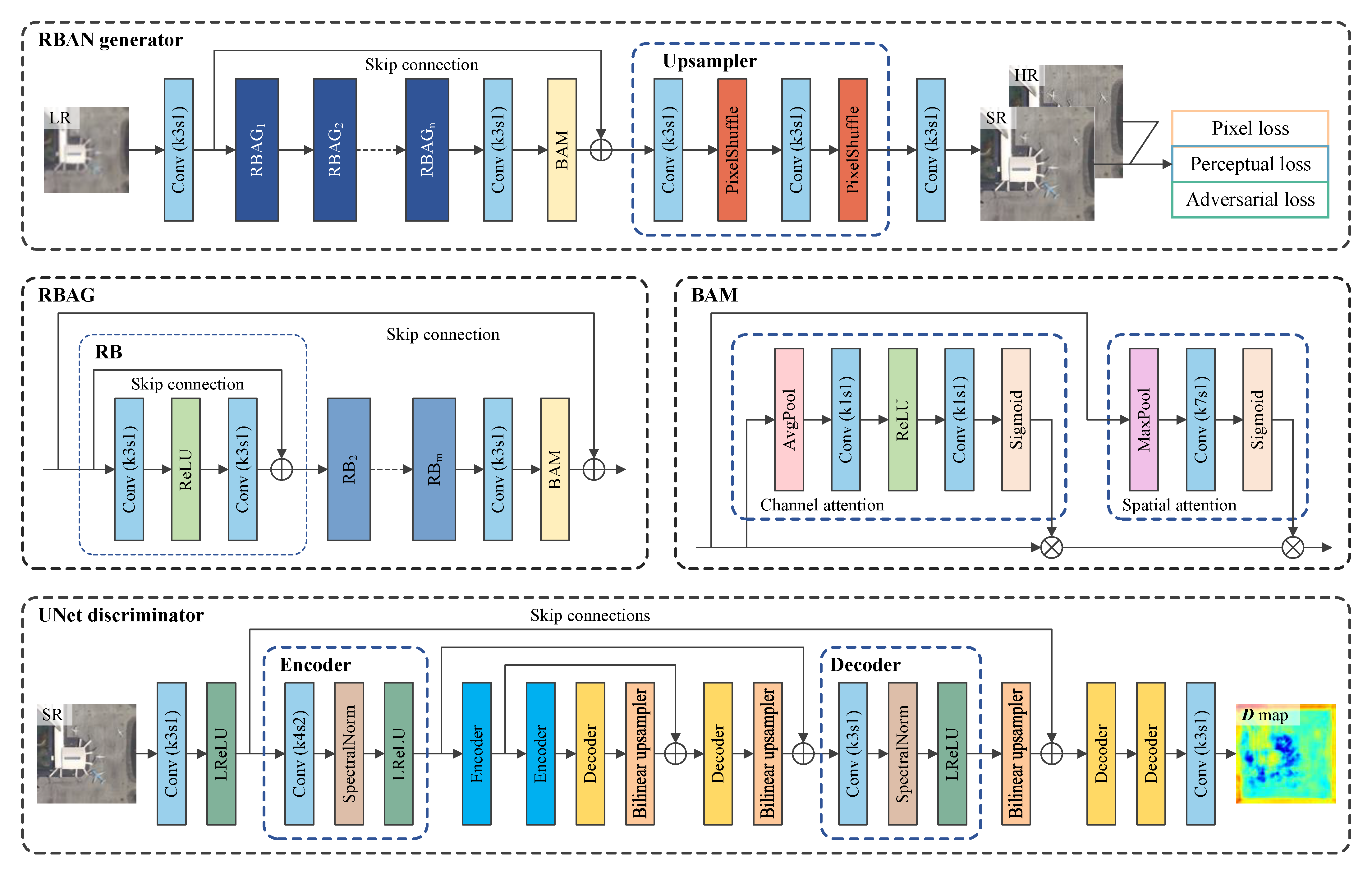
(1) Network architectures: Let us denote and as LR and HR image, respectively, where C, H, and W are the size of channel, height, and width respectively; s is the scale factor. The goal of the network is to obtain the SR estimation as close as the ground truth for a given LR input . As shown in Figure 4, the proposed RBAN model mainly consists of three parts: shallow feature extraction, deep feature extraction, and reconstruction.
At the beginning of the network, there is a convolutional layer for extracting shallow features from the LR input image. The mapping function of this part can be written as
where denotes the convolutional function with kernel size 3 and stride 1.
The deep feature extraction part is located after the shallow feature extraction part. It consists of multiple residual balanced attention groups (RBAG), one convolutional layer, and one balanced attention module (BAM). The deep feature extraction part has a skip connection to provide a shortcut from input to output, which is also known as the global residual strategy. In each RBAG, there are a group of basic residual blocks (RB), a convolutional layer and a BAM. There is also a skip connection from the input to the output of RBAG. The mapping function of the deep feature extraction part can be written as
where is the mapping function of RBAG, denotes the mapping function of BAM, and denotes the mapping function of ReLU activation layer. RB is the basic unit of SISR network, which usually consists of convolutional layers and activation layers, such as the batch normalization (BN) and the rectified linear unit (ReLU). In this work, we apply the RB structure that used in EDSR [30], which consists of a convolutional layer, a rectified linear unit (ReLU) and another convolutional layer in sequence. There is also a skip connection from the input to the output of RB. The mapping function of RB is formulated as
In the end, an upsampler and a convolutional layer make up the reconstruction part. The upsampler is used to upscale the feature maps from LR space to HR space. The upsamplers are different for different scale factors. As shown in Figure 4, two pixel shuffle layers and two convolutional layers are interleaved in a ×4 upsampler. A convolutional layer located after the upsampler converts the feature map into the SR image output. The mapping function of reconstruction part can be written as
where is the mapping function of the upsampler, denotes the mapping function of the pixel shuffle layer.
(2) Balanced attention module (BAM): Attention mechanism is an important strategy in SISR model, which emphasizes the different importance between channels or spatial locations by assigning weights to feature maps. To improve the performance of the model, we employ the balanced attention module (BAM) [43]. BAM models interdependence of different channels and spatial locations at the same time. The mapping functions of BAM can be written as
where denotes the map function of maximum pooling layer, denotes the map function of average pooling layer, denotes the convolutional function with kernel size 7 and stride 1, is the convolutional function with kernel size 1 and stride 1, is the sigmoid map function.
As shown in Figure 4, BAM contains two paths for channel attention and spatial attention, respectively. In the channel attention path, the input feature map is turned into a channel-wise feature map by the average pooling layer. Then, two convolutional layers and a sandwiched ReLU layer implement the ‘squeeze-and-excitation’ operation. Afterwards, the sigmoid layer turns the feature map into a channel-wise output weight vector. In the spatial attention path, the input feature map is turned into a spatial-wise feature map by the max pooling layer. Then, a convolutional layer and a sigmoid layer turn the feature map into a spatial-wise output weight vector. Finally, two output weight vectors are broadcast-multiplied with the input feature map to obtain the attention result.
(3) Discriminator Model: Adversarial learning is a strategy commonly used in recent models for realistic SISR results. These models are also known as generative adversarial networks (GAN). In standard GAN-based SR models, the generator model G is trained to produce HR estimations from input images such that the discriminator model D cannot distinguish them from ground-truth HR images.
In this article, we use the RBAN model as generator and employ a modified UNet discriminator as shown in Figure 4. The convolutional layer in the discriminator with a kernel size of 4 and a stride of 2 extracts features while downscaling the spatial resolution. Spectral normalization layers and leaky ReLU layers are used to ensure the training stability. ↑ denotes the upsample operation with bilinear interpolation. Different from the standard VGG-style discriminator that only estimates the realness of the whole image, the UNet-based discriminator estimates the realness of each pixel, which produces accurate gradient feedback for local textures.
We also enhance the discriminator with relativistic GAN (RGAN) [44] framework. Unlike D in standard GANs, which estimates the probability that an input image ( or ) is ground truth or estimated, D in RGAN predicts the probability that the ground-truth image is relatively more realistic than the estimated one . Assuming the discriminator output of standard GAN as
where is the sigmoid mapping function, is the non-transformed discriminator output. The discriminator output of RGAN is formulated as
where denotes taking average for all data in the mini-batch.
3.4. Loss Function
The objective of the SISR can be formulated as
where G is the generator model parameterized by , is the loss function of the generator, N is the number of training images, .
Considering the realistic degradation process, more effective constraints should be imposed on the network during training. Thus, we combine pixel loss, perceptual loss, and adversarial loss with weighted average. The synthetic loss is formulated as
where , and are the weight coefficients to balance three loss terms.
The pixel loss is to measure the pixel-wise difference between the ground-truth HR image and estimated SR image. It is the basic component of the loss function and plays an irreplaceable role in ensuring network convergence. We choose to use the function as the pixel loss, denoted as
where C, H, and W are the channel number, height, and width of the evaluated images, respectively.
The perceptual loss is to measure the differences between two images using features extracted with a pretrained 19-layer VGG network. As a commonly used image classification network, the pretrained VGG can extract high-level semantic information from input images, which helps to improve the quality of network output images. In this work, we use the VGG network truncated at the Conv5-4 layer to extract features and function to calculate the difference between feature maps
where is the map function of the truncated VGG network.
As for the adversarial loss, the loss functions are calculated under the RGAN framework, formulated as
where is the loss function of the discriminator.
4. Experiments and Analysis
4.1. Experimental Settings
(1) Datasets: In the experiments, we used three widely usedremote sensing datasets, including AID [15], UCMERCED [16], and RSIs-CB256 [17]. These datasets are all RGB image datasets originally used for aerial scene classification; therefore, these datasets contain a variety of scenes, such as oceans, lands mountains, and buildings, which are very suitable for evaluating the generalization ability of networks in practical conditions. AID contains 10,000 images of 600 × 600 pixels in 30 scenes, with resolutions ranging from 8 to 0.5 m. UCMERCED is a 21-class remote sensing image dataset. Each class consists of 100 images, each of which is of 256 × 256 pixels. RSIs-CB256 is a remote sensing image dataset with a spatial resolution of 0.3–3 m and a pixel size of 256 × 256. It contains 35 categories and more than 24,000 images.
We use AID to build the realistic training dataset considering that its image size is more suitable for the degradation modeling. At first, we use KernelGAN [21,22] to collect all possible blur kernels in AID to construct the blur kernel dataset . Secondly, we extract noise patches according to Equation (5) and construct the noise patch dataset . Then, we use AID, , and to generate the realistic training dataset according to Equations (2) and (3). The downsampling scales c and s in the experiments are 2 and 4, respectively. For each image, and are randomly selected to increase the diversity of training samples. Finally, we randomly select 9500 image pairs as the training dataset and 500 image pairs as the test dataset for referenced evaluation. To compare the performance of networks trained with realistic dataset and ideal dataset, we also build an ideal AID training dataset with bicubic downsampling. In the ‘ideal’ dataset, the 4× bicubic downsampled HR images are labeled as LR images. As for UCMERCED and RSIs-CB256, to reduce time consumption, we randomly select 500 images from UCMERCED and RSIs-CB256, respectively, for non-referenced evaluation. In other words, the images in the UCMERCED and RSIs-CB256 dataset are not downsampled but directly used as network input to generate the corresponding SR images.
(2) Implementation details: During the training phase, the LR images were randomly cropped to 48 × 48 as inputs, the super-resolution scale was 4×, and the batch size was set as 16. Image flips and rotations were randomly used for data augmentation. Both the proposed model and other compared methods were trained for 2 iterations (337 epochs) using the ADAM optimizer. We set , , and in ADAM. The learning rate was initialed as and halved every 2 iterations. The proposed model was implemented with PyTorch framework and trained on a NVIDIA GTX3090 GPU.
(3) Evaluation metrics: We employ 4 widely used referenced image quality assessment metrics including peak signal-to-noise ratio (PSNR) [45], structure similarity index (SSIM) [46], independent feature similarity (IFS) [47], and learned perceptual image patch similarity (LPIPS) [48] in this work. We also adopt 2 widely used non-referenced image quality assessment metrics including natural image quality evaluator (NIQE) [49] and entropy-based non-reference image quality assessment (ENIQA) [50] in this work. Since the main energy of images is concentrated in the low-frequency area pixel-wise referenced metrics such as PSNR and SSIM average differences per pixel, thereby focusing on the flat parts of the images. Feature-based metrics such as IFS and LPIPS calculate differences in the feature spaces, thereby paying more attention on the high-frequency components of images. Non-referenced metrics such as NIQE and ENIQA are also defined on feature spaces, thus they also focus on the edge parts of the images. To sum up, all these metrics are somewhat one-sided and require comprehensive consideration.
4.2. Experiments on Referenced Evaluation
(1) Setup: As there is no research that considers the degradation process for the SR of RSIs as far as we know, we compared the proposed method with 6 classic SISR networks, including SRCNN [24], VDSR [28], DDBPN [51], EDSR [30], SRGAN [29], and DRLN [32]. The bicubic interpolation was also used as a baseline. For a fair comparison, the non-GAN-based models were all trained with only the pixel loss, while SRGAN was trained with the same loss component weights mentioned in the original paper. Experimental results under 3 kinds of settings are provided to verify the effectiveness of the degradation modeling. The first setting was to train and test models on the ‘ideal’ AID dataset, where the LR images were downsampled with only bicubic interpolation, as denoted in Equation (1). The second setting was to train models on the ‘ideal’ AID dataset and test on the realistic AID dataset. The realistic dataset was built using the proposed degradation framework, as denoted in Equation (3). In the third setting, the models were trained and tested on the realistic AID dataset. In other words, in the first and second settings, the models were exactly the same but the test datasets were different. In the second and third settings, the test datasets were the same but the models were different.
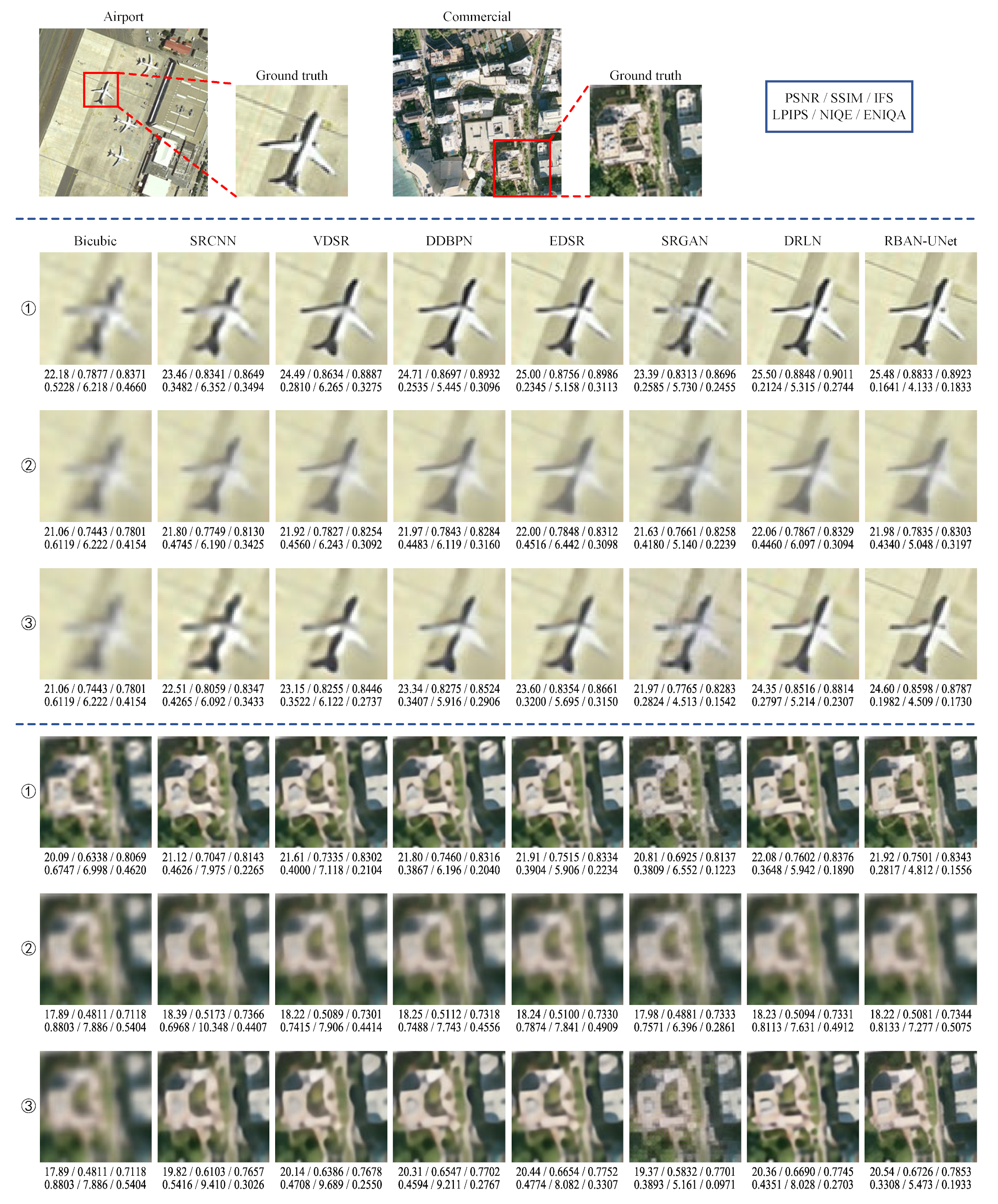
(2) Results: The average quantitative evaluation metrics of 8 methods on the AID dataset are shown in Table 1, where the first and second best results are marked in red and green, respectively. Visual examples and corresponding evaluation metrics are provided in Figure 5. Since both bicubic and realistic AID datasets are synthesized, all referenced and non-referenced metrics are provided. The experimental results can be interpreted from two perspectives.
First, comparing the metrics for all 3 settings, all methods perform worse in the second setting than in the first. There is significant blurring in the visualization of the second setting. This indicates that models trained on bicubic dataset do not generalize well to the actual degradation process such as blur and noise. Without considering degradation, CNN-based methods are not qualified for practical use in SISR of remote sensing images. Furthermore, as can be seen from Table 1 and Figure 5, all methods perform better in the third setting than in the second setting. This indicates that the proposed degradation modeling framework is rational and the estimation of blur and noise is effective. Models trained with realistic dataset do have better generalization abilities for the super resolution of real remote sensing images.
Second, comparing all 8 methods (focus on the 3rd setting), RBAN-UNet achieves the best performance. The bicubic upsample method achieves the worst performance because it uses information from a very limited neighborhood area to estimates unknown pixel values, and its interpolation operation process does not vary with the image content. SRCNN performs much better because its multi-layer convolutional structure forms a much larger receptive field and the non-linear mapping enables SRCNN to achieve better computation for different image content. Based on SRCNN, the global residual structure of VDSR make it possible to stack more convolutional layers, which is beneficial to improve the performance. DDBPN adopts an iterative upscale and downscale strategy and dense connections in the network, which enables it to learn the interdependencies between LR images and HR images and achieves a better performance. EDSR performs better than DDBPN because its local residual strategy and efficient residual block design enable its super deep structure. DRLN achieves the best performance on bicubic dataset but performs much worse on realistic dataset because it lacks a targeted design to deal with degradation factors. SRGAN achieve worse PSNR, SSIM, and IFS results than EDSR, but better LPIPS, NIQE, and ENIQA results, because SRGAN is trained with perceptual loss and GAN framework. This proves a fundamental fact that introducing more details into SR images can increase the perceptual performance and may lead to pixel-wise performance degradation. Another fact is that non-referenced metrics prefer images with more details, but at the same time, these metrics have difficulty distinguishing between natural details and artifacts. The SR results of SRGAN do have more details, but many of them are artifacts and can not substantially improve the quality of SR images. To sum up, the perceptual loss and GAN framework are double-edged swords for improving SR performance. As for the proposed method, RBAN can serve as a good backbone by using the residual in residual structure and the residual balanced attention mechanism. Based on RBAN and SRGAN, RBAN-UNet applies pixel loss to balance perceptual loss and adversarial loss and uses a modified UNet as the pixel-wise discriminator in RGAN framework. RBAN-UNet achieves 4 optimal and 2 sub-optimal among 6 metrics under the 3rd setting, which is the best performance in all comparison methods. It can also be seen from the visualization that the results of RBAN-UNet contain sharper edges but do not introduce invalid textures. RBAN-UNet finds a good balance between details and cleanliness. The effectiveness of the proposed model is verified.
4.3. Experiments on Non-Referenced Evaluation
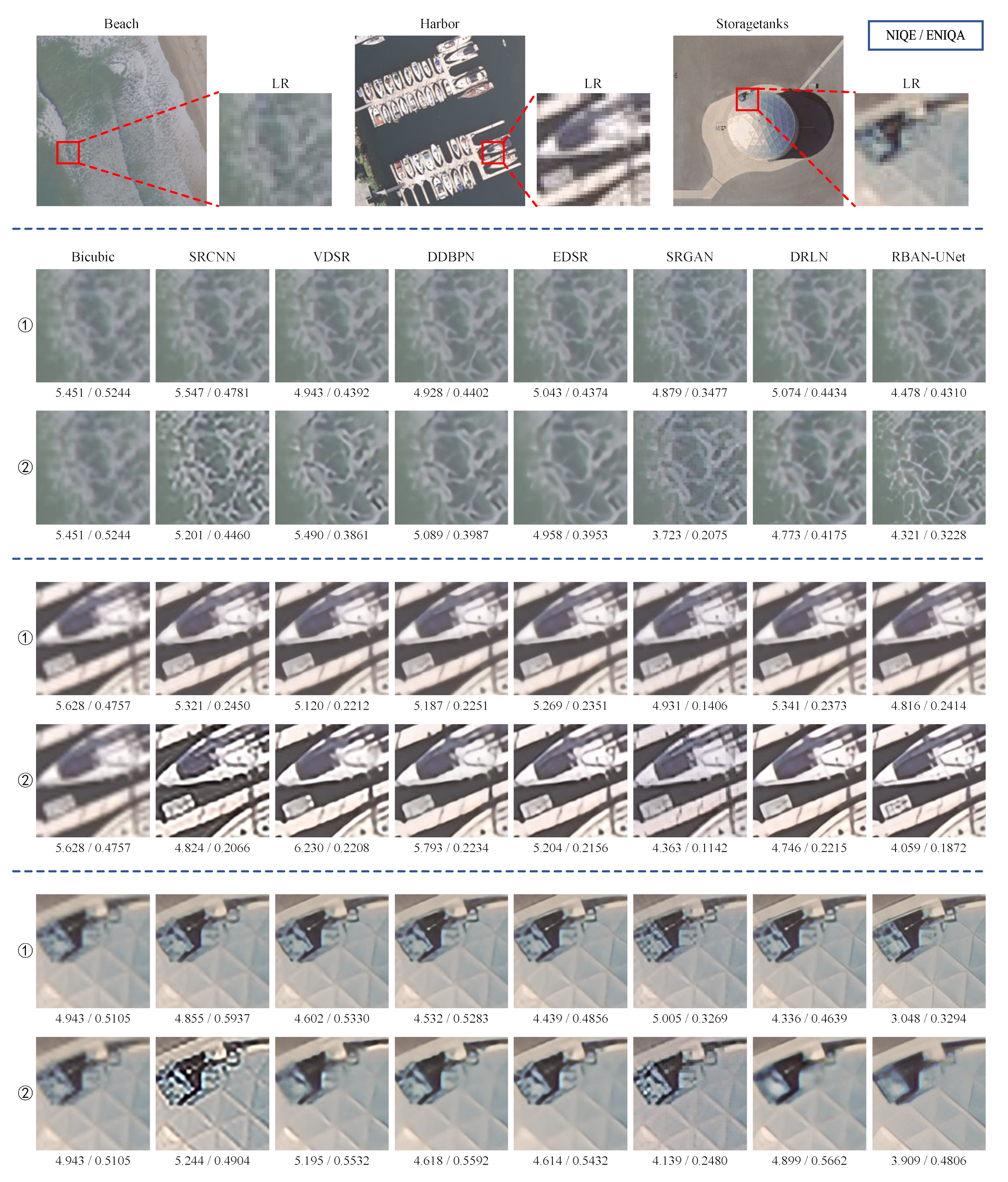
(1) Setup: In addition to the quantitative evaluation of all methods on the AID dataset using referenced metrics, we also evaluated all methods on the UCMERCED and RSIs-CB256 datasets. All methods were trained without any information from the UCMERCED and RSIs-CB256 datasets, which provides a good condition for evaluating the validity and generalization ability of all methods. Since the experiments were performed directly on the real images in UCMERCED and RSIs-CB256 datasets rather than the downsampled images, only non-referenced metrics are provided. The experiment results are provided with 2 kinds of settings: training on the ‘ideal’ AID dataset or realistic AID dataset.
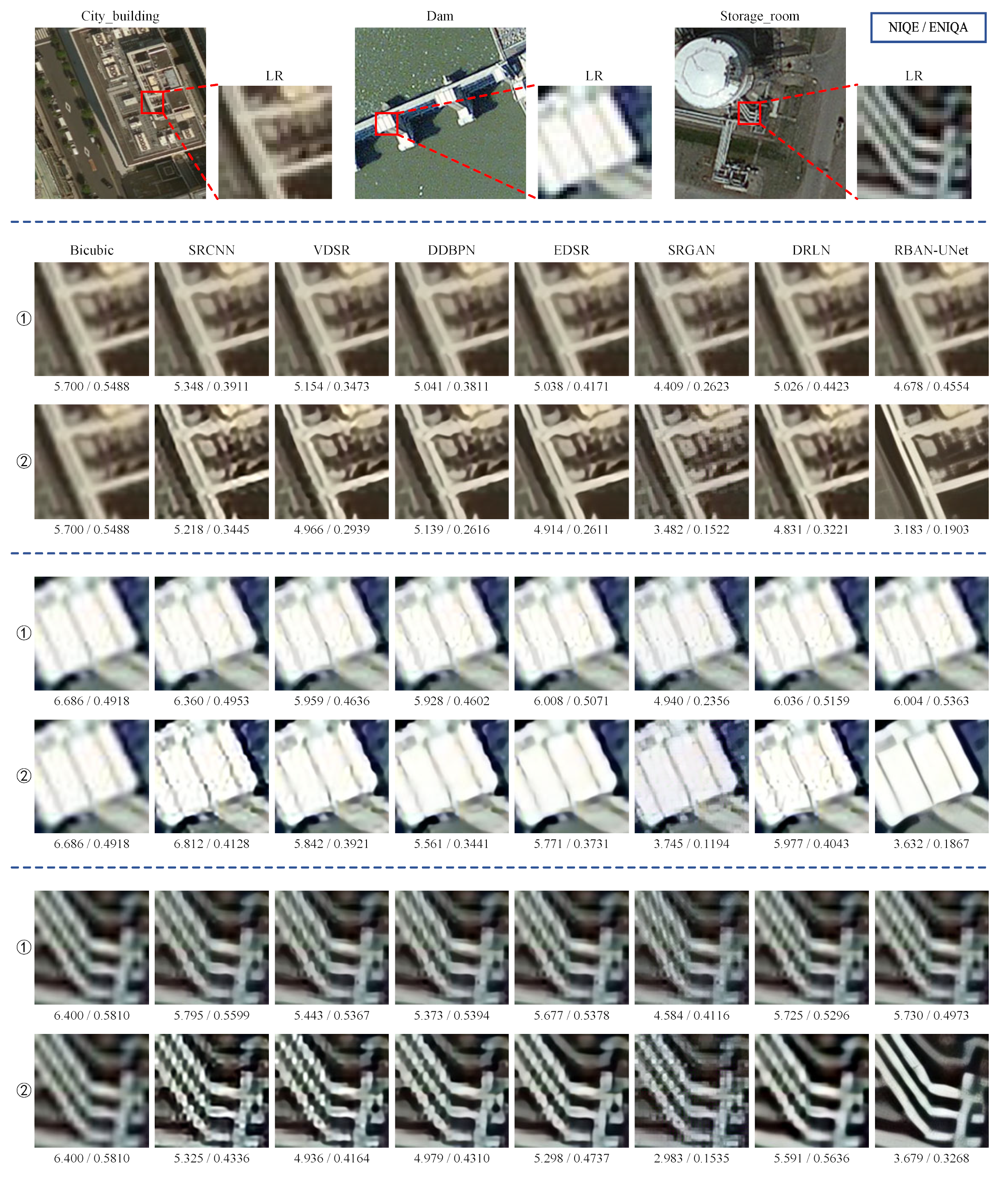
(2) Results: The average quantitative evaluation metrics and visualization of 8 methods tested on the UCMERCED dataset are shown in Table 2 and Figure 6, respectively. Models trained on the realistic AID dataset achieve higher metrics and better visualizations than models trained on bicubic AID dataset. This proves that the models do not overfit to the AID dataset and indeed gain generalization ability to deal with the degradation process. Horizontally comparing all 8 methods with the non-referenced metrics, SRGAN achieves the optimal metrics and RBAN-UNet achieves the sub-optimal metrics; however, as is mentioned above, NIQE and ENIQA are non-referenced feature-based image quality assessment metrics; therefore, images with more details, textures, and even artifacts are easy to achieve higher NIQE and ENIQA scores, which can be confirmed from the referenced evaluation experiments. From an intuitive point of view, SRGAN introduces lots of artifacts or invalid textures, which does not substantially improve the quality of reconstructed images; therefore, considering both visualization and non-reference metrics, it can be concluded that RBAN-UNet achieves the best performance on the UCMERCED dataset. The experiment results of RSIs-CB256 dataset shown in Table 3 and Figure 7 also support this conclusion. These experiments demonstrate that the proposed framework and model can effectively improve the performance of remote sensing image super resolution under practical conditions.
5. Discussion
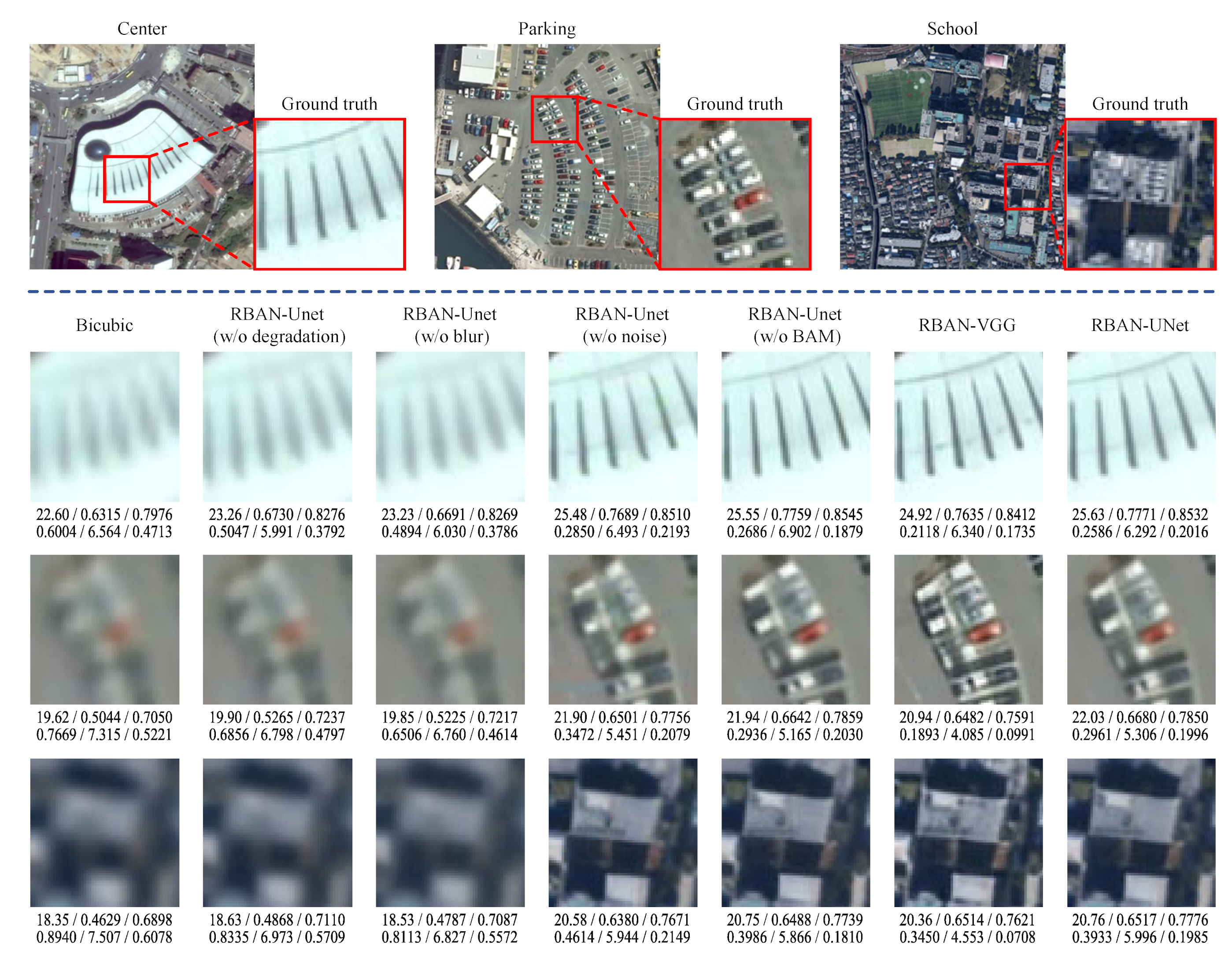
In addition, we conducted an ablation study to further discuss the effectiveness of each proposed component. The quantitative and visual results are shown in Table 4 and Figure 8, respectively.
5.1. Impact of Blur Kernel Estimation
As shown in Table 4 and Figure 8, RBAN-UNet (w/o degradation) achieves the worst performance among all discussed methods. RBAN-UNet (w/o degradation) denotes RBAN-UNet without any modeling of the blur and noise. It is equivalent to the model trained on bicubic dataset and tested on realistic dataset, as discussed in above subsections. RBAN-UNet (w/o noise) denotes RBAN-UNet without modeling the noise. It achieves much better metrics and sharper visual perception than RBAN-UNet (w/o degradation). Moreover, the complete RBAN-UNet outperforms RBAN-UNet (w/o blur) and the RBAN-UNet without modeling blur. These results confirm that the blur kernel estimation method is effective and the blur kernels help the networks to perform sharper super-resolution reconstructions.
5.2. Impact of Noise Patch Estimation
The complete RBAN-UNet model outperforms RBAN-UNet (w/o noise), which demonstrates the effectiveness of noise patch estimation and that the noise patches help the networks to perform better super-resolution reconstructions; however, there is no significant improvement in the results of RBAN-UNet (w/o blur) compared to RBAN-UNet (w/o degradation). We think the reason is that the influence of blur kernel exceeds that of noise patches.
5.3. Impact of BAM
The BAM that can be easily embedded in and removed from the model is a key component in the RBAN-UNet. As can be seen in Table 4 and Figure 8, removing BAMs from the model results in a significant drop in quantitative and perceptual performance when compared with the complete RBAN-UNet. This confirms the effectiveness and necessity of using BAM in network.
5.4. Impact of Discriminator
At last, we evaluated the function of the discriminator by replacing the discriminator in RBAN-UNet with VGG. Although RBAN-VGG achieves the best perceptual results, it introduces lots of invalid textures that are detrimental to understanding image content. RBAN-UNet achieves the best performance by comprehensively considering quantitative and perceptual results. It shows that the discriminator helps a lot to improve the perceptual performance, and the modified UNet achieves a better balance between quantitative and perceptual performances than VGG. The comparison confirms the effectiveness of the modified UNet discriminator.
6. Conclusions
In this article, a real-world degradation modeling framework and a residual balanced attention network with modified UNet discriminator (RBAN-UNet) have been proposed for remote sensing image super resolution. The quality of real RSIs is affected by a series of factors, such as illumination, atmosphere, imaging sensor responses, and signal processing, resulting in a gap in the performance of previous methods between laboratory conditions and actual conditions. To model the real-world degradation of RSIs, we propose to estimate the blur kernels and noise patches in the dataset separately. Then, the blur kernels and noise patches are used to construct a realistic dataset that follows the desired mapping function from realistic LR images to clean HR images. Moreover, we develop a novel CNN model to perform the SR reconstruction for RSIs. We use a residual in residual architecture as the backbone and embed balanced attention modules (BAM) to improve the performance. To generate more realistic results, a modified UNet pixel-wise discriminator is employed. Detailed experiments were carried out to compare the proposed model with classic SISR networks. Referenced experiments, non-referenced experiments, and ablation studies validate that the degradation modeling framework improves the performance of models dealing with real RSIs and the proposed RBAN-UNet model achieves a state-of-the-art performance in the real-world SISR problem for RSIs. In our future work, we will focus on decoupling the degradation and images inside the network instead of explicitly collecting the degradation datasets.
Author Contributions
Conceptualization, J.Z.; methodology, J.Z.; software, J.Z.; validation, J.Z., T.X. and J.L.; formal analysis, S.J.; investigation, Y.Z.; resources, T.X.; data curation, T.X.; writing—original draft preparation, J.Z.; writing—review and editing, J.L., S.J. and Y.Z.; visualization, J.Z.; supervision, T.X.; project administration, T.X. and J.L.; funding acquisition, J.Z. and T.X. All authors have read and agreed to the published version of the manuscript.
Funding
This work was supported by the National Natural Science Foundation of China (grant no. 61527802, 61371132, 61471043), China Postdoctoral Science Foundation (grant no. BX20200051), Natural Science Foundation of Chongqing (grant no. cstc2021jcyj-msxmX1130).
Data Availability Statement
The code will be available at https://github.com/zhangjizhou-bit/Single-image-Super-Resolution-of-Remote-Sensing-Images-with-Real-World-Degradation-Modeling, (accessed on 1 June 2022).
Conflicts of Interest
The authors declare no conflict of interest.
References
- Rau, J.Y.; Jhan, J.P.; Hsu, Y.C. Analysis of oblique aerial images for land cover and point cloud classification in an urban environment. IEEE Trans. Geosci. Remote Sens. 2014, 53, 1304–1319. [Google Scholar] [CrossRef]
- Lang, J.; Lyu, S.; Li, Z.; Ma, Y.; Su, D. An investigation of ice surface albedo and its influence on the high-altitude lakes of the Tibetan Plateau. Remote Sens. 2018, 10, 218. [Google Scholar] [CrossRef]
- Voigt, S.; Kemper, T.; Riedlinger, T.; Kiefl, R.; Scholte, K.; Mehl, H. Satellite image analysis for disaster and crisis-management support. IEEE Trans. Geosci. Remote Sens. 2007, 45, 1520–1528. [Google Scholar] [CrossRef]
- Ghaffarian, S.; Kerle, N.; Filatova, T. Remote sensing-based proxies for urban disaster risk management and resilience: A review. Remote Sens. 2018, 10, 1760. [Google Scholar] [CrossRef] [Green Version]
- Romero, A.; Gatta, C.; Camps-Valls, G. Unsupervised deep feature extraction for remote sensing image classification. IEEE Trans. Geosci. Remote Sens. 2015, 54, 1349–1362. [Google Scholar] [CrossRef] [Green Version]
- Roy, P.S.; Roy, A.; Joshi, P.K.; Kale, M.P.; Srivastava, V.K.; Srivastava, S.K.; Dwevidi, R.S.; Joshi, C.; Behera, M.D.; Meiyappan, P.; et al. Development of decadal (1985–1995–2005) land use and land cover database for India. Remote Sens. 2015, 7, 2401–2430. [Google Scholar] [CrossRef] [Green Version]
- Wang, Z.; Chen, J.; Hoi, S.C. Deep Learning for Image Super-resolution: A Survey. IEEE Trans. Pattern Anal. Mach. Intell. 2020, 43, 3365–3387. [Google Scholar] [CrossRef] [Green Version]
- Wei, P.; Lu, H.; Timofte, R.; Lin, L.; Zuo, W.; Pan, Z.; Li, B.; Xi, T.; Fan, Y.; Zhang, G.; et al. AIM 2020 challenge on real image super-resolution: Methods and results. In Proceedings of the European Conference on Computer Vision, Glasgow, UK, 23–28 August 2020; Springer: Cham, Swizerland, 2020; pp. 392–422. [Google Scholar]
- Bhat, G.; Danelljan, M.; Timofte, R. NTIRE 2021 challenge on burst super-resolution: Methods and results. In Proceedings of the IEEE/CVF Conference on Computer Vision and Pattern Recognition, Nashville, TN, USA, 20–25 June 2021; pp. 613–626. [Google Scholar]
- Yue, L.; Shen, H.; Li, J.; Yuan, Q.; Zhang, H.; Zhang, L. Image super-resolution: The techniques, applications, and future. Signal Process. 2016, 128, 389–408. [Google Scholar] [CrossRef]
- Chen, H.; He, X.; Qing, L.; Wu, Y.; Ren, C.; Sheriff, R.E.; Zhu, C. Real-world single image super-resolution: A brief review. Inf. Fusion 2022, 79, 124–145. [Google Scholar] [CrossRef]
- McKinley, S.; Levine, M. Cubic spline interpolation. Coll. Redwoods 1998, 45, 1049–1060. [Google Scholar]
- Lu, T.; Wang, J.; Zhang, Y.; Wang, Z.; Jiang, J. Satellite image super-resolution via multi-scale residual deep neural network. Remote Sens. 2019, 11, 1588. [Google Scholar] [CrossRef] [Green Version]
- Xiong, Y.; Guo, S.; Chen, J.; Deng, X.; Sun, L.; Zheng, X.; Xu, W. Improved SRGAN for remote sensing image super-resolution across locations and sensors. Remote Sens. 2020, 12, 1263. [Google Scholar] [CrossRef] [Green Version]
- Xia, G.S.; Hu, J.; Hu, F.; Shi, B.; Bai, X.; Zhong, Y.; Zhang, L.; Lu, X. AID: A benchmark data set for performance evaluation of aerial scene classification. IEEE Trans. Geosci. Remote Sens. 2017, 55, 3965–3981. [Google Scholar] [CrossRef] [Green Version]
- Yang, Y.; Newsam, S. Bag-of-visual-words and spatial extensions for land-use classification. In Proceedings of the 18th SIGSPATIAL International Conference on Advances in Geographic Information Systems, San Jose, CA, USA, 2–5 November 2010; pp. 270–279. [Google Scholar]
- Li, H.; Dou, X.; Tao, C.; Wu, Z.; Chen, J.; Peng, J.; Deng, M.; Zhao, L. RSI-CB: A large-scale remote sensing image classification benchmark using crowdsourced data. Sensors 2020, 20, 1594. [Google Scholar] [CrossRef] [Green Version]
- Zhang, S.; Yuan, Q.; Yuan, Q.; Li, J.; Sun, J.; Zhang, X. Scene-adaptive remote sensing image super-resolution using a multiscale attention network. IEEE Trans. Geosci. Remote Sens. 2020, 58, 4764–4779. [Google Scholar] [CrossRef]
- Zhang, X.; Li, Z.; Zhang, T.; Liu, F.; Tang, X.; Chen, P.; Jiao, L. Remote Sensing Image Super-Resolution via Dual-Resolution Network Based on Connected Attention Mechanism. IEEE Trans. Geosci. Remote Sens. 2021, 60, 5611013. [Google Scholar] [CrossRef]
- Zhang, D.; Shao, J.; Li, X.; Shen, H.T. Remote Sensing Image Super-Resolution via Mixed High-Order Attention Network. IEEE Trans. Geosci. Remote Sens. 2021, 59, 5183–5196. [Google Scholar] [CrossRef]
- Bell-Kligler, S.; Shocher, A.; Irani, M. Blind super-resolution kernel estimation using an internal-GAN. Adv. Neural Inf. Process. Syst. 2019, 32, 1–10. [Google Scholar]
- Ji, X.; Cao, Y.; Tai, Y.; Wang, C.; Li, J.; Huang, F. Real-world super-resolution via kernel estimation and noise injection. In Proceedings of the IEEE Computer Society Conference on Computer Vision and Pattern Recognition Workshops, Seattle, WA, USA, 14–19 June 2020; pp. 1914–1923. [Google Scholar]
- Liang, J.; Cao, J.; Sun, G.; Zhang, K.; Van Gool, L.; Timofte, R. SwinIR: Image Restoration Using Swin Transformer. In Proceedings of the 2021 IEEE/CVF International Conference on Computer Vision Workshops (ICCVW), Montreal, BC, Canada, 11–17 October 2021; IEEE: Piscataway, NJ, USA, 2021; pp. 1833–1844. [Google Scholar]
- Dong, C.; Loy, C.C.; He, K.; Tang, X. Learning a deep convolutional network for image super-resolution. In Proceedings of the European Conference on Computer Vision, Zurich, Switzerland, 6–12 September 2014; Springer: Cham, Switzerland, 2014; pp. 184–199. [Google Scholar]
- Zeyde, R.; Elad, M.; Protter, M. On single image scale-up using sparse-representations. In Proceedings of the International Conference on Curves and Surfaces, Avignon, France, 24–30 June 2010; Springer: Berlin/Heidelberg, Germany; pp. 711–730.
- Timofte, R.; De Smet, V.; Van Gool, L. Anchored neighborhood regression for fast example-based super-resolution. In Proceedings of the IEEE International Conference on Computer Vision, Sydney, Australia, 1–8 December 2013; pp. 1920–1927. [Google Scholar]
- Caballero, J.; Ledig, C.; Aitken, A.; Acosta, A.; Totz, J.; Wang, Z.; Shi, W. Real-time video super-resolution with spatio-temporal networks and motion compensation. In Proceedings of the IEEE Conference on Computer Vision and Pattern Recognition, Honolulu, HI, USA, 21–26 July 2017; pp. 4778–4787. [Google Scholar]
- Kim, J.; Lee, J.K.; Lee, K.M. Accurate Image Super-Resolution Using Very Deep Convolutional Networks. In Proceedings of the 2016 IEEE Conference on Computer Vision and Pattern Recognition (CVPR), Las Vegas, NV, USA, 27–30 June 2016; IEEE: Piscataway, NJ, USA, 2016; Volume 60, pp. 1646–1654. [Google Scholar]
- Ledig, C.; Theis, L.; Huszár, F.; Caballero, J.; Cunningham, A.; Acosta, A.; Aitken, A.; Tejani, A.; Totz, J.; Wang, Z.; et al. Photo-realistic single image super-resolution using a generative adversarial network. In Proceedings of the 30th IEEE Conference on Computer Vision and Pattern Recognition, CVPR 2017, Honolulu, HI, USA, 21–26 July 2017; pp. 105–114. [Google Scholar]
- Lim, B.; Son, S.; Kim, H.; Nah, S.; Lee, K.M. Enhanced Deep Residual Networks for Single Image Super-Resolution. In Proceedings of the 2017 IEEE Conference on Computer Vision and Pattern Recognition Workshops (CVPRW), Honolulu, HI, USA, 21–26 July 2017; IEEE: Piscataway, NJ, USA, 2017; pp. 1132–1140. [Google Scholar]
- Zhang, Y.; Li, K.; Li, K.; Wang, L.; Zhong, B.; Fu, Y. Image Super-Resolution Using Very Deep Residual Channel Attention Networks. In Encyclopedia of Signaling Molecules; Springer: New York, NY, USA, 2018; pp. 294–310. [Google Scholar]
- Anwar, S.; Barnes, N. Densely residual laplacian super-resolution. IEEE Trans. Pattern Anal. Mach. Intell. 2020, 44, 1192–1204. [Google Scholar] [CrossRef]
- Zhang, X.; Chen, Q.; Ng, R.; Koltun, V. Zoom to learn, learn to zoom. In Proceedings of the IEEE/CVF Conference on Computer Vision and Pattern Recognition, Long Beach, CA, USA, 15–20 June 2019; pp. 3762–3770. [Google Scholar]
- Yuan, Y.; Liu, S.; Zhang, J.; Zhang, Y.; Dong, C.; Lin, L. Unsupervised image super-resolution using cycle-in-cycle generative adversarial networks. In Proceedings of the IEEE Conference on Computer Vision and Pattern Recognition Workshops, Salt Lake City, UT, USA, 18–22 June 2018; pp. 701–710. [Google Scholar]
- Nguyen, N.; Milanfar, P. A wavelet-based interpolation-restoration method for superresolution (wavelet superresolution). Circuits Syst. Signal Process. 2000, 19, 321–338. [Google Scholar] [CrossRef]
- Li, F.; Jia, X.; Fraser, D.; Lambert, A. Super resolution for remote sensing images based on a universal hidden Markov tree model. IEEE Trans. Geosci. Remote Sens. 2009, 48, 1270–1278. [Google Scholar]
- Pan, Z.; Yu, J.; Huang, H.; Hu, S.; Zhang, A.; Ma, H.; Sun, W. Super-resolution based on compressive sensing and structural self-similarity for remote sensing images. IEEE Trans. Geosci. Remote Sens. 2013, 51, 4864–4876. [Google Scholar] [CrossRef]
- Lei, S.; Shi, Z.; Zou, Z. Super-resolution for remote sensing images via local–global combined network. IEEE Geosci. Remote Sens. Lett. 2017, 14, 1243–1247. [Google Scholar] [CrossRef]
- Jiang, K.; Wang, Z.; Yi, P.; Jiang, J.; Xiao, J.; Yao, Y. Deep distillation recursive network for remote sensing imagery super-resolution. Remote Sens. 2018, 10, 1700. [Google Scholar] [CrossRef] [Green Version]
- Ma, W.; Pan, Z.; Guo, J.; Lei, B. Achieving super-resolution remote sensing images via the wavelet transform combined with the recursive res-net. IEEE Trans. Geosci. Remote Sens. 2019, 57, 3512–3527. [Google Scholar] [CrossRef]
- Guo, M.; Zhang, Z.; Liu, H.; Huang, Y. NDSRGAN: A Novel Dense Generative Adversarial Network for Real Aerial Imagery Super-Resolution Reconstruction. Remote Sens. 2022, 14, 1574. [Google Scholar] [CrossRef]
- Michaeli, T.; Irani, M. Nonparametric blind super-resolution. In Proceedings of the IEEE International Conference on Computer Vision, Sydney, Australia, 1–8 December 2013; pp. 945–952. [Google Scholar]
- Wang, F.; Hu, H.; Shen, C. BAM: A Balanced Attention Mechanism for Single Image Super Resolution. arXiv 2021, arXiv:2104.07566. [Google Scholar]
- Jolicoeur-Martineau, A. The relativistic discriminator: A key element missing from standard GAN. In Proceedings of the International Conference on Learning Representations, Vancouver, BC, Canada, 30 April–3 May 2018. [Google Scholar]
- Huynh-Thu, Q.; Ghanbari, M. Scope of validity of PSNR in image/video quality assessment. Electron. Lett. 2008, 44, 800–801. [Google Scholar] [CrossRef]
- Hore, A.; Ziou, D. Image quality metrics: PSNR vs. SSIM. In Proceedings of the 2010 20th International Conference on Pattern Recognition, Istanbul, Turkey, 23–26 August 2010; IEEE: Piscataway, NJ, USA, 2010; pp. 2366–2369. [Google Scholar]
- Chang, H.w.; Zhang, Q.w.; Wu, Q.g.; Gan, Y. Perceptual image quality assessment by independent feature detector. Neurocomputing 2015, 151, 1142–1152. [Google Scholar] [CrossRef]
- Zhang, R.; Isola, P.; Efros, A.A.; Shechtman, E.; Wang, O. The unreasonable effectiveness of deep features as a perceptual metric. In Proceedings of the IEEE Conference on Computer Vision and Pattern Recognition, Salt Lake City, UT, USA, 18–22 June 2018; pp. 586–595. [Google Scholar]
- Mittal, A.; Soundararajan, R.; Bovik, A.C. Making a “completely blind” image quality analyzer. IEEE Signal Process. Lett. 2012, 20, 209–212. [Google Scholar] [CrossRef]
- Chen, X.; Zhang, Q.; Lin, M.; Yang, G.; He, C. No-reference color image quality assessment: From entropy to perceptual quality. EURASIP J. Image Video Process. 2019, 2019, 1–14. [Google Scholar] [CrossRef] [Green Version]
- Haris, M.; Shakhnarovich, G.; Ukita, N. Deep back-projection networks for super-resolution. In Proceedings of the IEEE Conference on Computer Vision and Pattern Recognition, Salt Lake City, UT, USA, 18–22 June 2018; pp. 1664–1673. [Google Scholar]
Figure 1.
Framework of real-world degradation modeling. Remote sensing images in the original dataset are not paired. First, the blur kernels and noise patches are collected from the original dataset, forming and . Then, the paired dataset is generated using , and real RSIs. At last, a novel network is trained to estimate SR results from LR inputs.

Figure 2.
Blur kernel estimation with KernelGAN. D tries to differentiate between real patches and those generated by G (fake). G learns to downsample the image while fooling D.
Figure 2.
Blur kernel estimation with KernelGAN. D tries to differentiate between real patches and those generated by G (fake). G learns to downsample the image while fooling D.

Figure 3.
Noise patches extraction from real RSIs.

Figure 4.
Network architectures of the residual balanced attention network (RBAN) generator and the modified UNet discriminator. The basic unit of RBAN is the residual balanced attention group (RBAG), which is mainly composed of a group of residual blocks (RB). The balanced attention module (BAM) is an essential component in RBAN and RBAG to improve performance. The modified UNet model is employed as a pixel-wise discriminator for more realistic reconstructions. It consists of multiple encoders and decoders to extract and reconstruct features at multiple scales.

Figure 5.
Visual comparison and assessment metrics of the proposed model and 7 other methods on 2 test images from the AID dataset, “airport_15” and “commercial_67”, at a ×4 scale factor. The performances are compared under 3 settings: ① train and test on bicubic AID dataset, ② train on bicubic AID dataset and test on realistic AID dataset, and ③ train and test on realistic AID dataset. Since both the bicubic and realistic AID dataset are synthesized, all referenced and non-referenced metrics are provided.

Figure 6.
Visual comparison and assessment metrics of the proposed model and the other eight methods on three test images from the UCMERCED dataset, “beach30”, “harbor69”, and “storagetanks87”, at ×4 scale. The performances are compared under 2 settings: ① trained on bicubic AID dataset and test on realistic UCMERCED dataset; ② trained on realistic AID dataset and tested on realistic UCMERCED dataset. As the images from UCMERCED dataset were directly used for test without downsampling, only non-referenced metrics are provided.

Figure 7.
Visual comparison and assessment metrics of the proposed model and the other eight methods on three test images from the RSIs-CB256 dataset, “city_building(57)”, “dam(83)”, and “storage_room(715)”, at ×4 scale. The performances are compared under 2 settings: ① trained on bicubic AID dataset and tested on realistic RSIs-CB256 dataset; ② trained on realistic AID dataset and tested on realistic RSIs-CB256 dataset. As the images RSIs-CB256 dataset were directly used for test without downsampling, only non-referenced metrics are provided.

Figure 8.
Visual comparison and assessment metrics of the ablation study models on three test images from the AID dataset, “center_233”, “parking_226”, and “school_33”, at ×4 scale.
Figure 8.
Visual comparison and assessment metrics of the ablation study models on three test images from the AID dataset, “center_233”, “parking_226”, and “school_33”, at ×4 scale.


Table 1.
Quantitative evaluation results of all methods on the AID dataset with three settings.
| Train | Test | Methods | PSNR↑ | SSIM↑ | IFS↑ | LPIPS↓ | NIQE↓ | ENIQA↓ |
|---|---|---|---|---|---|---|---|---|
| Bicubic AID | Bicubic AID | Bicubic | 25.73 | 0.7267 | 0.8416 | 0.5532 | 6.402 | 0.4534 |
| SRCNN [24] | 26.54 | 0.7670 | 0.8629 | 0.4309 | 7.412 | 0.3288 | ||
| VDSR [28] | 27.00 | 0.7861 | 0.8736 | 0.3805 | 7.140 | 0.2815 | ||
| DDBPN [51] | 27.10 | 0.7906 | 0.8759 | 0.3741 | 6.854 | 0.2836 | ||
| EDSR [30] | 27.24 | 0.7960 | 0.8794 | 0.3688 | 6.739 | 0.2862 | ||
| SRGAN [29] | 26.10 | 0.7527 | 0.8605 | 0.3273 | 6.307 | 0.1720 | ||
| DRLN [32] | 27.43 | 0.8034 | 0.8822 | 0.3499 | 6.706 | 0.2702 | ||
| RBAN-UNet | 27.25 | 0.7944 | 0.8752 | 0.2710 | 5.318 | 0.2082 | ||
| Bicubic AID | Realistic AID | Bicubic | 23.65 | 0.6332 | 0.7417 | 0.7207 | 7.112 | 0.5602 |
| SRCNN [24] | 23.93 | 0.6483 | 0.7556 | 0.6478 | 7.663 | 0.5053 | ||
| VDSR [28] | 23.90 | 0.6479 | 0.7563 | 0.6493 | 7.425 | 0.5077 | ||
| DDBPN [51] | 23.91 | 0.6484 | 0.7570 | 0.6486 | 7.207 | 0.5143 | ||
| EDSR [30] | 23.91 | 0.6485 | 0.7576 | 0.6600 | 7.360 | 0.5217 | ||
| SRGAN [29] | 23.64 | 0.6338 | 0.7576 | 0.6270 | 5.615 | 0.4188 | ||
| DRLN [32] | 23.92 | 0.6488 | 0.7584 | 0.6672 | 7.265 | 0.5274 | ||
| RBAN-UNet | 23.88 | 0.6468 | 0.7570 | 0.6552 | 6.683 | 0.5349 | ||
| Realistic AID | Realistic AID | Bicubic | 23.65 | 0.6332 | 0.7417 | 0.7207 | 7.112 | 0.5602 |
| SRCNN [24] | 24.81 | 0.6926 | 0.7803 | 0.5607 | 7.398 | 0.4013 | ||
| VDSR [28] | 25.14 | 0.7109 | 0.7936 | 0.4921 | 8.266 | 0.3299 | ||
| DDBPN [51] | 25.29 | 0.7180 | 0.8009 | 0.4827 | 7.915 | 0.3337 | ||
| EDSR [30] | 25.45 | 0.7250 | 0.8079 | 0.4750 | 7.404 | 0.3462 | ||
| SRGAN [29] | 24.14 | 0.6649 | 0.7877 | 0.3749 | 4.547 | 0.1647 | ||
| DRLN [32] | 24.83 | 0.7038 | 0.7840 | 0.5523 | 7.497 | 0.3814 | ||
| RBAN-UNet | 25.68 | 0.7336 | 0.8160 | 0.3548 | 5.736 | 0.2462 |
The first and second best metrics are marked in red and green respectively. ↑ denotes the higher the better and ↓ denotes the lower the better.
Table 2.
Quantitative evaluation results of all eight methods on the UCMERCED dataset with two settings.
Table 2.
Quantitative evaluation results of all eight methods on the UCMERCED dataset with two settings.
| Train | Methods | NIQE↓ | ENIQA↓ |
|---|---|---|---|
| Bicubic AID | Bicubic | 6.362 | 0.5368 |
| SRCNN [24] | 7.431 | 0.4336 | |
| VDSR [28] | 7.337 | 0.4073 | |
| DDBPN [51] | 7.265 | 0.4064 | |
| EDSR [30] | 6.848 | 0.4209 | |
| SRGAN [29] | 5.719 | 0.2827 | |
| DRLN [32] | 6.400 | 0.4219 | |
| RBAN-UNet | 5.237 | 0.3827 | |
| Realistic AID | Bicubic | 6.362 | 0.5368 |
| SRCNN [24] | 7.940 | 0.3907 | |
| VDSR [28] | 6.295 | 0.3791 | |
| DDBPN [51] | 6.085 | 0.3646 | |
| EDSR [30] | 5.961 | 0.3909 | |
| SRGAN [29] | 4.329 | 0.1516 | |
| DRLN [32] | 7.033 | 0.4091 | |
| RBAN-UNet | 4.709 | 0.3169 |
The first and second best metrics are marked in red and green respectively. ↑ denotes the higher the better and ↓ denotes the lower the better.
Table 3.
Quantitative evaluation results of all eight methods on the RSIs-CB256 dataset with two settings.
Table 3.
Quantitative evaluation results of all eight methods on the RSIs-CB256 dataset with two settings.
| Train | Methods | NIQE↓ | ENIQA↓ |
|---|---|---|---|
| Bicubic AID | Bicubic | 6.896 | 0.5670 |
| SRCNN [24] | 6.424 | 0.4941 | |
| VDSR [28] | 6.169 | 0.4876 | |
| DDBPN [51] | 6.091 | 0.4908 | |
| EDSR [30] | 6.159 | 0.5011 | |
| SRGAN [29] | 5.453 | 0.4019 | |
| DRLN [32] | 6.133 | 0.5003 | |
| RBAN-UNet | 5.308 | 0.5393 | |
| Realistic AID | Bicubic | 6.896 | 0.5670 |
| SRCNN [24] | 6.780 | 0.4452 | |
| VDSR [28] | 6.194 | 0.4462 | |
| DDBPN [51] | 6.178 | 0.4475 | |
| EDSR [30] | 6.426 | 0.4847 | |
| SRGAN [29] | 3.979 | 0.2143 | |
| DRLN [32] | 6.123 | 0.4917 | |
| RBAN-UNet | 4.953 | 0.4369 |
The first and second best metrics are marked in red and green respectively. ↑ denotes the higher the better and ↓ denotes the lower the better.
Table 4.
Ablation results of RBAN-UNet on the realistic AID dataset.
| Models | PSNR↑ | SSIM↑ | IFS↑ | LPIPS↓ | NIQE↓ | ENIQA↓ |
|---|---|---|---|---|---|---|
| Bicubic | 23.652 | 0.6332 | 0.7417 | 0.7207 | 7.112 | 0.5602 |
| RBAN-UNet (w/o degradation) | 23.885 | 0.6468 | 0.7570 | 0.6552 | 6.683 | 0.5349 |
| RBAN-UNet (w/o blur) | 23.722 | 0.6411 | 0.7528 | 0.6316 | 6.649 | 0.5335 |
| RBAN-UNet (w/o noise) | 24.980 | 0.7053 | 0.7876 | 0.4403 | 5.239 | 0.2739 |
| RBAN-UNet (w/o BAM) | 25.610 | 0.7310 | 0.8137 | 0.3602 | 5.745 | 0.2487 |
| RBAN-VGG | 25.029 | 0.7186 | 0.8000 | 0.2722 | 4.877 | 0.1454 |
| RBAN-UNet | 25.676 | 0.7336 | 0.8160 | 0.3548 | 5.736 | 0.2462 |
The first and second best metrics are marked in red and green respectively. ↑ denotes the higher the better and ↓ denotes the lower the better.
Publisher’s Note: MDPI stays neutral with regard to jurisdictional claims in published maps and institutional affiliations. |
© 2022 by the authors. Licensee MDPI, Basel, Switzerland. This article is an open access article distributed under the terms and conditions of the Creative Commons Attribution (CC BY) license (https://creativecommons.org/licenses/by/4.0/).
Share and Cite
MDPI and ACS Style
Zhang, J.; Xu, T.; Li, J.; Jiang, S.; Zhang, Y. Single-Image Super Resolution of Remote Sensing Images with Real-World Degradation Modeling. Remote Sens. 2022, 14, 2895. https://doi.org/10.3390/rs14122895
AMA Style
Zhang J, Xu T, Li J, Jiang S, Zhang Y. Single-Image Super Resolution of Remote Sensing Images with Real-World Degradation Modeling. Remote Sensing. 2022; 14(12):2895. https://doi.org/10.3390/rs14122895
Chicago/Turabian StyleZhang, Jizhou, Tingfa Xu, Jianan Li, Shenwang Jiang, and Yuhan Zhang. 2022. "Single-Image Super Resolution of Remote Sensing Images with Real-World Degradation Modeling" Remote Sensing 14, no. 12: 2895. https://doi.org/10.3390/rs14122895
Note that from the first issue of 2016, this journal uses article numbers instead of page numbers. See further details here.