Article

High Spatial Resolution Fractional Vegetation Coverage Inversion Based on UAV and Sentinel-2 Data: A Case Study of Alpine Grassland

1
College of Geomatics and Geoinformation, Guilin University of Technology, Guilin 541004, China
2
Guangxi Key Laboratory of Spatial Information and Geomatics, Guilin University of Technology, Guilin 541004, China
3
School of Geographic Sciences, Nantong University, Nantong 226007, China
4
State Key Laboratory of Cryospheric Sciences, Northwest Institute of Eco-Environment and Resources, Chinese Academy of Sciences, Lanzhou 730000, China
*
Author to whom correspondence should be addressed.
Remote Sens. 2023, 15(17), 4266; https://doi.org/10.3390/rs15174266
Submission received: 22 July 2023 / Revised: 24 August 2023 / Accepted: 29 August 2023 / Published: 30 August 2023

Abstract

:
Fractional vegetation coverage (FVC) is an important indicator of ecosystem change. At present, FVC products are mainly concentrated at low and medium spatial resolution and lack high temporal and spatial resolution, which brings certain challenges to the fine monitoring of ecological environments. In this study, we evaluated the accuracy of four remote sensing inversion models for FVC based on high-spatial-resolution Sentinel-2 imagery and unmanned aerial vehicle (UAV) field-measured FVC data in 2019. Then the inversion models were optimized by constructing a multidimensional feature dataset. Finally, the Source Region of the Yellow River (SRYR) FVC product was created using the best inversion model, and the spatial-temporal variation characteristics of the FVC in the region were analyzed. The study’s findings revealed that: (1) The accuracies of the four FVC inversion models were as follows: the Gradient Boosting Decision Tree (GBDT) model (R2 = 0.967, RMSE = 0.045) > Random Forest (RF) model (R2 = 0.962, RMSE = 0.049) > Support Vector Machine (SVM) model (R2 = 0.925, RMSE = 0.072) > Pixel Dichotomy (PD) model (R2 = 0.869, RMSE = 0.097). (2) Constructing a multidimensional feature dataset to optimize the driving data can improve the accuracy of the inversion model. NDVI and elevation are important factors affecting the accuracy of machine learning inversion algorithms, and the visible blue band is the most important feature factor of the GBDT model. (3) The FVC in the SRYR gradually increased from west to east and from north to south. The change trajectories of grassland FVC from 2017 to 2022 were not significant. The areas that tend to improve were mainly distributed in the southeast (1.31%), while the areas that tend to degrade were mainly distributed in the central and northwest (1.89%). This study provides a high-spatial-resolution FVC inversion optimization scheme, which is of great significance for the fine monitoring of alpine grassland ecological environments.

1. Introduction

Fractional Vegetation Cover (FVC) represents the proportion of vegetation area, encompassing leaves, stems, and branches, on the vertical projection surface relative to the total area of the specified region [1]. FVC can directly reflect the degree of regional greening and is an important parameter for monitoring ecological changes, characterizing the quality of vegetation, and evaluating soil erosion and desertification [2]. Its dynamic changes are related to the security and stability of the ecosystem and the integrity of its services and functions, so the accurate acquisition of FVC information is of great significance for ecological environment monitoring and related simulation studies.
Remote sensing technology is the main technical means for FVC inversion at regional and global scales due to its wide coverage and repeated monitoring [3]. Presently, FVC satellite remote sensing inversion methods predominantly fall into three categories: regression model approaches founded on vegetation indices, the Pixel dichotomy (PD) model, and machine learning algorithms. Among them, the machine learning algorithms obtain the best-fitting relationship by simulating the internal relationship between satellite remote sensing signals (reflectance data of each band or other relevant data) and real FVC (usually replaced by measured FVC or FVC product data) and then inverting FVC by using the relationship. Due to its ability to handle multidimensional variables, massive data, complex problems, and reflect the physical characteristics of remote sensing signals and real FVC to a certain extent [4], it has become a research hotspot for remote sensing inversion of ecological parameters, and it is commonly used to produce FVC product data on a global or regional scale. Commonly used machine learning algorithms include the Neural Network Algorithm [5], Support Vector Machine (SVM) [6], Classification and Regression Tree (CART) [7], and Random Forest (RF) [4]. However, the reflectance data of remote sensing images is frequently utilized as the input for FVC inversion without considering the ecological background or spatial heterogeneity. In addition, Lin et al. [2] showed that the inversion of FVC in alpine grassland is affected by a variety of environmental factors, among which topography and climate have a greater influence on FVC, but there are few studies on this part. It is necessary to further clarify the characteristics of the inversion accuracy based on the response of the environmental factors and optimize the inversion scheme.
At present, satellite remote sensing data is widely utilized to generate FVC product data, often employing machine learning algorithms or the PD model (e.g., GEOV1, GEOV2, GEOV3, GLASS, MuSyQ) (Table 1). The product data of GEOV1, GEOV2 and GEOV3 are all derived from the Copernicus Global Land Service (CGLS) [8]. The spatial resolution for GEOV1, GEOV2 and GEOV3 are approximately 1 km, 1 km and 300 m, respectively. Temporal resolution stands at 10 days, spanning from 1999 to 2020, 1999 to 2020, and 2014 to the present, respectively. GEOV2 enhances accuracy and spatial-temporal continuity by integrating climatological data with the base of GEOV1. Conversely, GEOV3 exhibits comparatively diminished spatial-temporal continuity due to the absence of climatological data for contextualization. All three products, GEOV1, GEOV2, and GEOV3, are produced using the Neural Network algorithm. The GLASS vegetation coverage data [9,10] is sourced from Beijing Normal University’s website and comprises two distinct product categories. Generalized Regression Neural Network models are trained using Landsat TM/ETM+ and MODIS reflectance data (MOD09A1) to produce global FVC product data. The resultant spatial resolution is 500 m, and the temporal resolution is 8 days, spanning from 2000 to 2020. A second product utilizes AVHRR sensor data, boasting a spatial resolution of 0.05°, an 8-day time step, and a time span from 1984 to 2020. The MuSyQ FVC product [11] boasts the highest temporal resolution among FVC products. With a spatial resolution of 500 m and a time resolution of 4 days, this product is founded on the porosity algorithm. Other researchers have also leveraged machine learning algorithms and FVC product data in their investigations. For example, Ge et al. [12] used MODIS data to invert the FVC in the SRYR and monitored its spatial distribution and dynamic changes; Yang et al. [13] verified the inconsistency and spatial-temporal discontinuity of the existing FVC products and produced global FVC product data based on MODIS data; Huang et al. [14] evaluated the spatiotemporal differences of four sets of FVC products in the ecological environment assessment of the three-rivers source region, and found that only 30% of the areas had the same change trend of the four sets of products, indicating that these FVC products have great uncertainty in the alpine grassland region. However, most of the current FVC product data were established using medium and low-resolution satellite image data, and FVC estimate models based on high-spatial-resolution remote sensing image data are also in short supply [5,13]. Existing studies have shown that remote sensing images with high-spatial-resolution can provide detailed surface feature information and capture finer details [15], such as vegetation canopy structure, leaf size and shape, topography, etc., helping to distinguish different types of vegetation and the FVC characteristics they belong to [16]. At the same time, high-spatial resolution remote sensing images can provide accurate information about the spatial distribution of FVC in a given area and can effectively capture small changes in vegetation [17]. Therefore, high spatial resolution can contribute to the extraction of vegetation information and capture fine-scale changes in FVC. In addition, medium and low resolution satellite remote sensing pixels are mostly mixed pixels, which are easy to introduce certain uncertainties to the inversion results and are not conducive to obtaining accurate vegetation monitoring data, whereas high spatial resolution remote sensing imagery can reduce the problem of mixed pixels, which can help to improve the accuracy of FVC inversion [16,18]. Therefore, in order to better monitor the ecological environment, there is an urgent need to enhance the production of high-spatiotemporal-resolution FVC product datasets.
Accurate FVC field measurements are critical for validating and evaluating inversion model methods. On the one hand, constructing high-quality inversion models requires reliable measurement data; on the other hand, the evaluation of the prediction results of the existing models requires accurate field-measured data as validation [19]. The current field ground survey methods mainly include visual inspection methods, sampling methods, and photography methods [20]. The visual inspection method is to estimate the FVC by visual judgment directly based on experience, and the results are more subjective. The sampling method uses grid point sampling to record surface FVC, which has high accuracy but is time-consuming and laborious. The photography method is based on taking photographs vertically using a digital camera above the sample plots, and then using image processing software to interpret these photographs and obtain FVC data [19]. Although the ground survey method can obtain the ground-measured data more accurately, it is difficult to match the pixel scale of the satellite remote sensing image in the spatial scale, which brings uncertainty to the satellite remote sensing inversion and verification. Chen et al. [19,21] found that UAV can well fill the uncertainty caused by traditional ground surveys “with points and areas”, and is an ideal tool for field FVC surveys. Because the image acquired by the UAV has high resolution and wide coverage, it can effectively solve the problem of spatial pixel matching between ground surveys and satellite remote sensing images. At the same time, UAV also has the advantages of small size, light weight, low cost, simple operation, rapid and accurate observation of sample sites, and effective acquisition of vegetation information for satellite remote sensing images at the pixel level, which can be used for large-scale field surveys of FVC and thus provide simulation and verification data for FVC inversion.
The Source Region of the Yellow River (SRYR) is located in the northeast of the Qinghai-Tibet Plateau, which is an important ecological barrier, water conservation area, and animal husbandry base in China. The region is characterized by high altitude, topographic relief, extremely variable precipitation and temperature, and intense solar radiation [12], resulting in a fragile and sensitive environment for vegetation growth. Over the past decades, under the impact of climate change, human activities, and pika infestation, the ecological environment of the region has undergone significant changes, posing great challenges to the sustainable development of the local and surrounding areas. Therefore, it is urgent to produce a high spatiotemporal resolution FVC dataset in this region to provide effective and accurate data support for local ecological environment fine monitoring and ecological protection policies. This study is based on Sentinel-2 images and a large number of measured FVC data points that match the spatial scale of Sentinel-2 images. The research objectives are as follows: evaluating the accuracy of FVC inversion with different machine learning algorithms; constructing a multidimensional feature dataset and optimizing the existing algorithms; based on the optimized algorithm, we produced a dataset of FVC in the SRYR, and evaluated the spatial-temporal variation of FVC in this region.

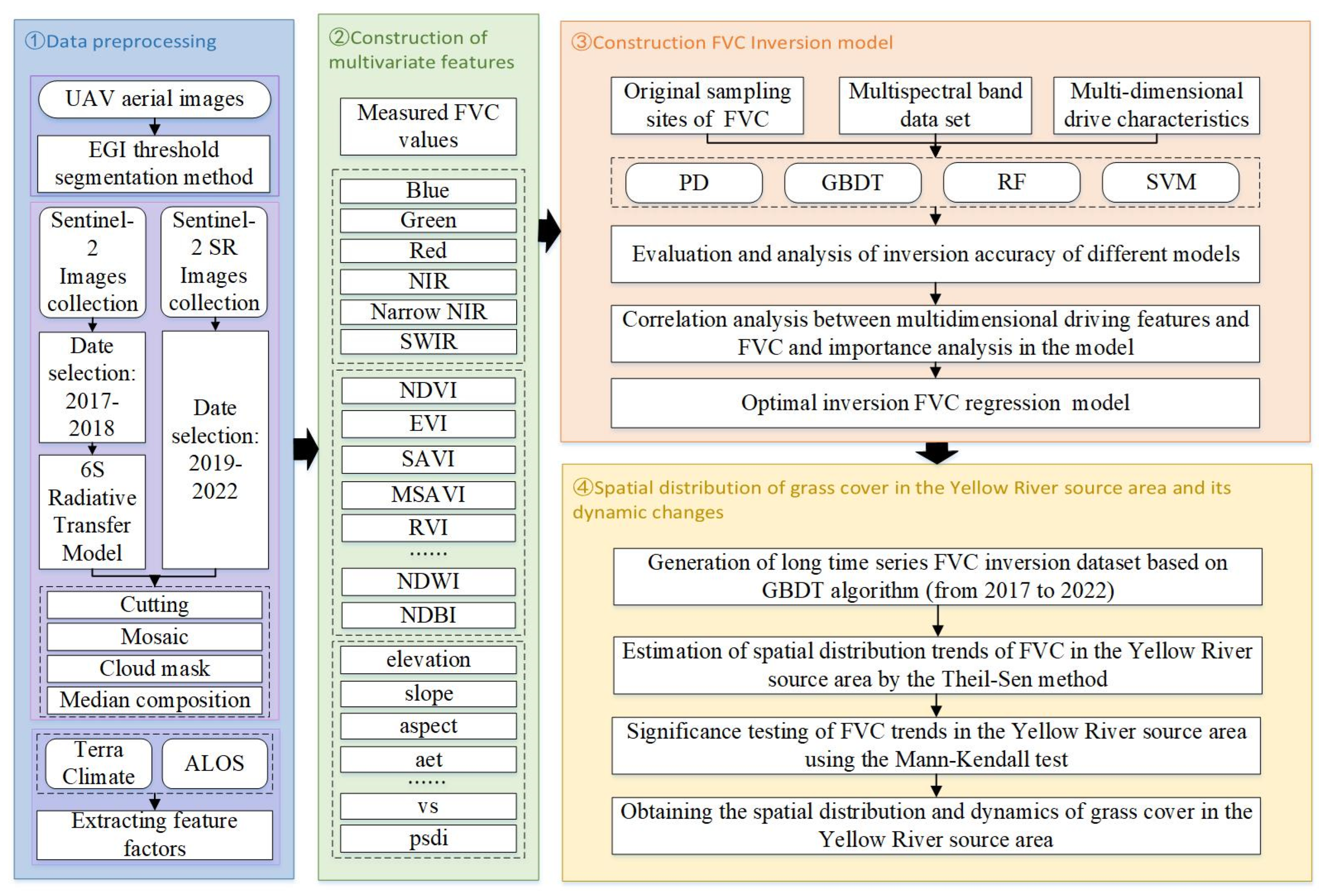
2. Materials and Methods
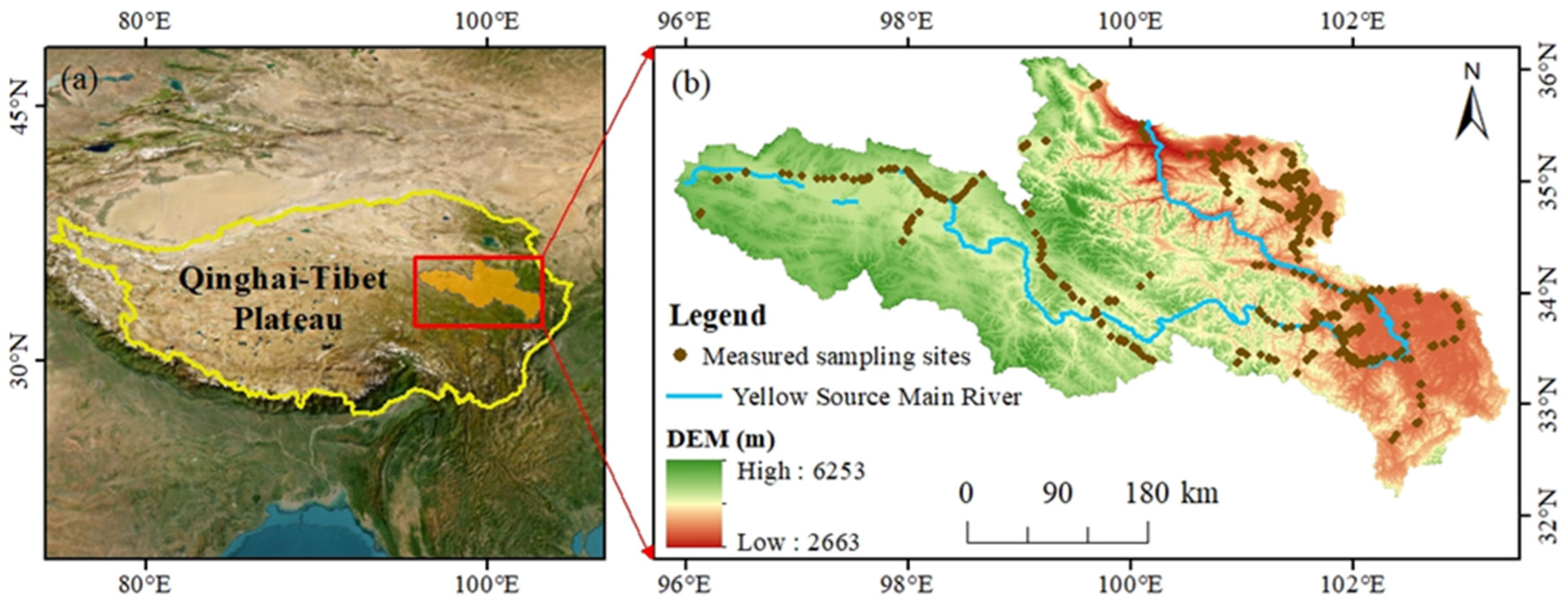
2.1. Study Area

The SRYR spans Gansu, Qinghai, and Sichuan provinces in China, located between 95.83°~103.50°E and 32.75°~36.85°N, with a total area of about 132,000 square kilometers. The average elevation is above 4000 m, and the terrain gradually increases from southeast to northwest (Figure 1). The climate type is subtropical and semi-humid, with an average annual temperature of −4~2° and an average annual precipitation of about 420 mm. The region is sensitive to climate change and ecologically fragile. The vegetation in this region is dominated by alpine meadows, alpine grasslands and alpine shrubs, and the vegetation species are relatively simple. The SRYR is the Yellow River Basin’s primary flow-producing area, water source area, and ecological conservation area, and it is an important ecological protection barrier, economic zone, and “energy basin” in China [2], which plays a pivotal role in agricultural production, water security, and ecological protection in the middle and lower reaches of the basin and the north of the country.

2.2. Data Source and Pre-Processing

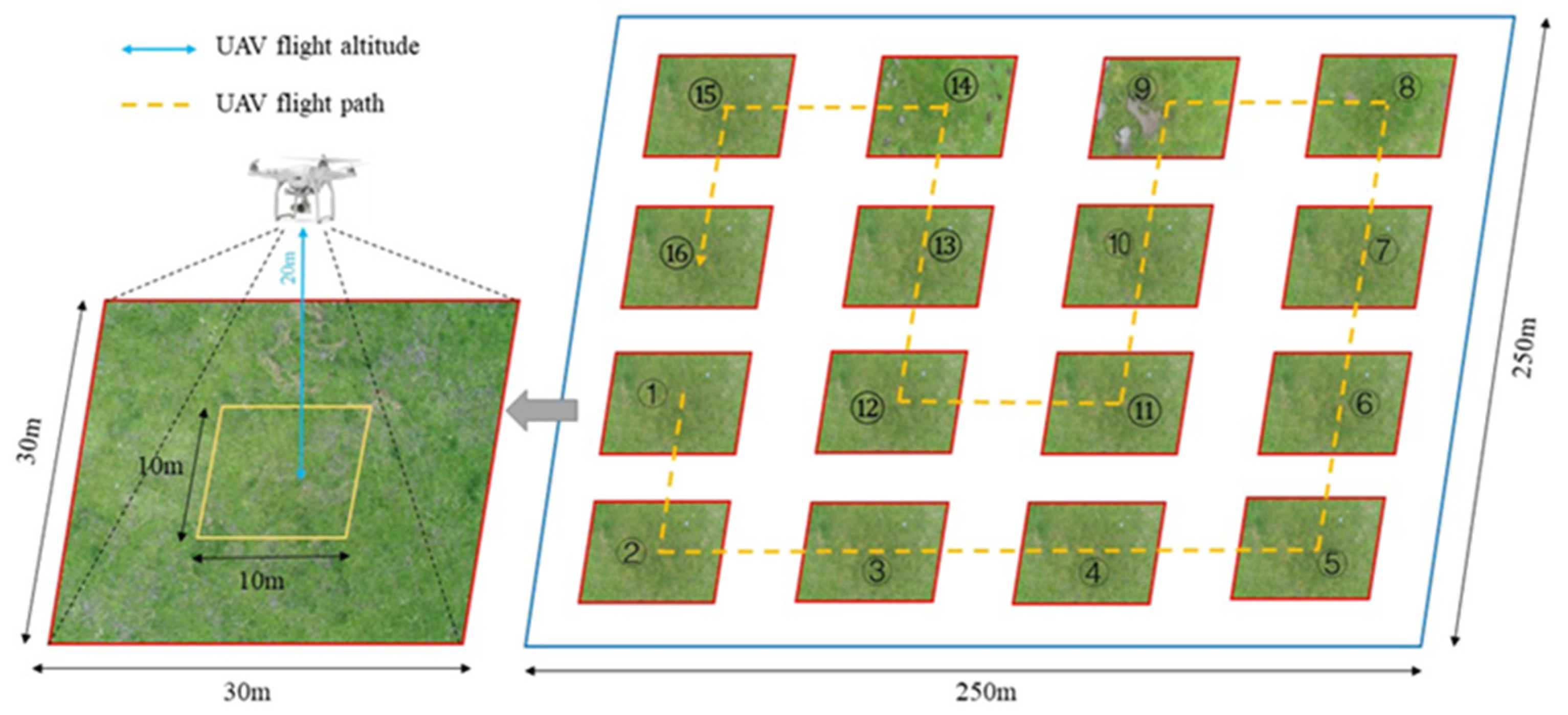
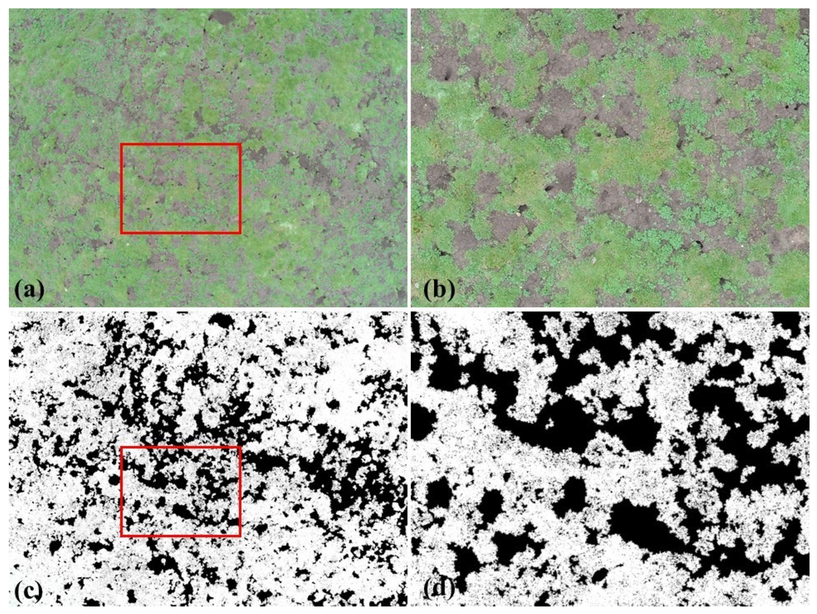
2.2.1. Field Data Based on UAV

We delineated 530 250 m × 250 m remote sensing monitoring sites in the study area during the prime time for vegetation growth from July to August 2019. Remote sensing monitoring sites have taken into account different grassland types, FVC, and different underlying surfaces and environmental conditions, so the monitoring sites are very representative of the study area. At each monitoring site, 16 additional 30 m ×30 m sample quadrats were uniformly laid out. Fragmentation Monitoring and Analysis with aerial Photography (FragMAP) [2,19] was utilized to set up routes and control the UAV to take photos vertically downward right above each sample square to obtain the sample-scale aerial images (Figure 2). The UAV used in this study was the Phantom 4 Professional four-axis unmanned aerial vehicle (http://www.dji.com. Accessed on 1 October 2021.) produced by DJI Innovation Technology Co., Ltd. (Shenzhen, China). The UAV is equipped with an augmentation head and a 1-inch CMOS sensor to acquire aerial images containing information in the red, green, and blue bands and store them in JPEG format with an effective pixel count of 20 million.
The aerial image obtained through UAV utilization employs the Excess Green Index (EGI) threshold method (EGI = 2G-R-B, where G, R, and B respectively denote the gray values of the green, red, and blue bands in the image) for FVC extraction. The procedure is delineated as follows: Commencing with the calculation of the EGI for each pixel within the aerial image, an initial EGI threshold is established. This preliminary value typically resides within the range of 40 to 160 in increments of 1, guided by insights from Lin et al. and Chen et al.’s [2,19,21] research. After careful analysis, we determined that the optimal threshold value for our study was 80, which resulted in the best correspondence between FVC extraction and the original image. The determination of the EGI threshold is conducted through the employment of the Java-based FVC Estimator software and remains adaptable, rather than being set at a fixed value [21]. Second, if an image element’s EGI value is higher than the threshold, it is categorized as a green vegetation element; otherwise, it is described as a non-vegetation element (Figure 3). Third, to assess the classification’s accuracy, the classification result is subsequently placed over the original image. If it is inaccurate, then readjust the initial threshold and repeat the above steps until the classification is accurate [2]. Finally, the FVC of the image was established by computing the proportion of vegetation pixels relative to the total pixel count. To assess the precision of the FVC yielded through this method, each image underwent analysis by two distinct individuals. Subsequently, the outcomes generated by these two assessors were juxtaposed and scrutinized. If the divergence in FVC measurements between the two analysts exceeded 0.05, a third proficient researcher undertook iterative image processing until alignment with the prescribed accuracy was achieved. This measure was implemented to mitigate the potential impact of human subjectivity on the extraction of FVC information from images [19,22]. UAV aerial images can clearly reflect the growth status of local vegetation, which is available for the acquisition of real FVC data.

2.2.2. Sentinel-2 Data

The Sentinel-2 satellite has an orbital altitude of 786 km and carries sensors covering 13 spectral bands, of which four bands, namely, blue, green, red and near-infrared, are imaged with a spatial resolution of 10 m. Sentinel-2 has a revisit period of 10 days for a single satellite and 5 days for a constellation of two A/B satellites. The Sentinel-2 data used in this paper were derived from the apparent reflectance image dataset (Level-1C product) and orthophoto dataset (Level-2A product) provided by the Google Earth Engine (GEE) platform. Among these, the image data from 2017 to 2018 were derived from the Level-1C product image set. To achieve atmospheric correction, the Py6S atmospheric correction module within the GEE platform was invoked on the image dataset. Py6S facilitates the configuration of 6S input parameters, simulation execution, and result retrieval through simple Python scripts, The utilization of Py6S ensures compatibility with the GEE platform and effectively addresses the atmospheric correction needs of Sentinel-2 Level1C data [23,24]. The 2019~2022 image data are based on the platform’s Level-2A product dataset, which has been atmospherically corrected by GEE platform using a set of lookup tables generated by libRadtran [24].

2.2.3. Other Supporting Data

The auxiliary data used in this study mainly include meteorological and topographic data, all of which were obtained from the GEE platform. The meteorological data used was TerraClimate (https://www.climatologylab.org/terraclimate.html. Accessed on 1 March 2022.). Using climate-assisted interpolation, TerraClimate creates monthly global land surface climate and climate water balance datasets, fusing the WorldClim dataset with the Climatic Research Unit gridded Time Series version 4.0 (CRU Ts4.0) and the Japanese 55-year Reanalysis (JRA55) datasets. The dataset covers meteorological data from 1958 to the present, including observations from weather stations, satellite measurements and reanalysis models.
The topographic data used was the ALOS 12.5 m DEM data (https://www.eorc.jaxa.jp/ALOS/en/url_change_info_e.htm. Accessed on 1 March 2022.), which is the elevation data produced by the Japan Aerospace Exploration Agency (JAXA) using the Advanced Land Observing Satellite (ALOS) phased-array type L-band synthetic aperture radar (PALSAR), which has three modes of observation: high-resolution, scanning synthetic aperture radar, and polarization. The horizontal and vertical accuracy of ALOS DEM elevation data is up to 12.5 m.

2.3. Research Methods

The research methods and technical flow are shown in Figure 4. It mainly includes the following technical modules:
① The field FVC data collected by UAV in the SRYR in 2019 was used as the sample data, containing data from 6028 monitoring sites.
② The multispectral reflectance dataset and multidimensional feature dataset were established using the GEE platform. The multispectral reflectance dataset contained only the information of multispectral bands (green (B2), blue (B3), red (B4), NIR (B8), Narrow NIR (B8A), SWIR (B11)) of the Sentinel-2 image. Given the susceptibility of vegetation growth in alpine regions to factors like altitude climate, we incorporated not only commonly used multi-spectral band information and vegetation indices but also accounted for altitude and climate attributes when constructing our multidimensional feature dataset. Furthermore, while vegetation indices like NDVI, EVI, SAVI, and MSAVI are indicative of vegetation growth conditions, they exhibit certain limitations such as susceptibility to soil background effects or insufficient sensitivity to vegetation growth. As a result, we extended our selection to include supplementary indices like LSWI, NDWI, IBI and NDBI. For instance, in the case of LSWI, its calculation leverages the red-edge band, which exhibits heightened sensitivity to vegetation variations and distinct mutation patterns at 770 nm, facilitating the extraction of FVC [25]. NDWI, on the other hand, enables the mitigation of cloud and snow interference to a certain degree [26]. IBI and NDBI were chosen for their capacity to account for impermeable surface and its influence. So the multidimensional feature dataset contained the information of multispectral bands (green, blue, red, NIR, Narrow NIR, SWIR), a variety of indices (NDVI, EVI, SAVI, MSAVI, RVI, DVI, IBI, LSWI, NDWI, NDBI), topography (elevation, slope, aspect), and temperature and precipitation (actual evapotranspiration (aet), precipitation (pr), drought index (pdsi), wind speed (vs)) data. The GEE platform facilitates the extraction of band and parameter information from Sentinel-2 images as well as terrain and climate data. Leveraging this platform, we retrieve the essential data components required for our analysis. The specific formula is shown in Table 2.
③ The PD model and machine learning algorithm models (SVM, RF, and GBDT) were used as the inversion model of FVC, and the sample points were randomly divided, with 70% of the dataset utilized for training and 30% for validation. Coefficient of determination (R2) and root mean square error (RMSE) were used to evaluate the accuracy of the inversion of the multispectral reflectance dataset and multidimensional feature dataset. The importance of each driving feature factor in the machine learning algorithm models and the correlation coefficient with the FVC were calculated to optimize the FVC inversion model.
④ The optimization model was used to simulate the FVC in the study area for 6 years (2017–2022). The spatial distribution and trend changes of FVC were obtained using the Theil-Sen (Sen) slope estimation method, and the Mann-Kendall (MK) significance test was performed for trend analysis.

2.3.1. The Pixel Dichotomy Model (PD)

The pixel dichotomy model (PD) assumes that the pixel is only composed of vegetation and non-vegetation, and the spectral information is linearly synthesized by these two components. The area proportion of each component in the pixel is the weight of each factor, and the percentage of the pixel covered by vegetation is the pixel of the FVC [1,2]. The formula is:
F V C = N D V I N D V I s o i l N D V I v e g N D V I s o i l
where: N D V I v e g is the N D V I value of pure vegetation pixel; N D V I s o i l is the N D V I value of pure bare soil pixel. In this study, 5% and 95% were chosen as the confidence intervals to determine N D V I v e g and N D V I s o i l .

2.3.2. Machine Learning Models

For all machine learning algorithm models, the input layer is the multispectral reflectance dataset or the multidimensional feature dataset, and the desired output is the FVC results. Initially, as a preprocessing step, we normalized all feature values in the dataset, including original spectral bands, multiple indices, and climatic topographic factors. Next, we randomly split the dataset into two portions: 70% for training and 30% for validation. Then, the machine learning algorithms were trained with the training dataset to establish the intrinsic relationship between the dataset and the FVC measurements. In the end, a test training set based on skilled machine learning methods is used to evaluate and validate the FVC inversion accuracy.
(1) Support Vector Machine (SVM)
Support Vector Machine (SVM) is a machine learning model based on statistical learning theory. The main idea is to map the input data to a high-dimensional space through a kernel function to achieve linear regression and build a linear decision function in the high-dimensional space. SVM is robust to outliers, has good generalization ability, and has high prediction accuracy, but it is not suitable for large datasets and performs poorly when the data sets contain a lot of noise [6,12,35].
In this study, the LIBSVM toolkit is invoked, which contains functions such as support vector regression. The SVM set type is e-SVR, the kernel function set type is radial basis function (RBF), the loss function P is 0.01, the RBF kernel parameter (GAMMA) is 0.3, and the penalty coefficient Cost is 6.
(2) Random Forest Model (RF)
The Random Forest model (RF) is an integrated learning algorithm that consists of multiple decision trees. The main idea is to take the decision tree as a weak model and use multiple decision trees for random sampling and joint predictions to improve model accuracy [36,37]. In the regression model, RF takes the average of the predicted values of multiple decision trees as the final prediction result, which has good practicability in the high-dimensional characteristic environment [36]. This algorithm is simple, fast, easy to implement, and avoids overfitting to a certain extent [2]. In this study, the RF regression algorithm provided by the GEE platform was invoked, and numberOfTrees was set to 900 and seed to 10.
(3) Gradient Boosting Decision Tree (GBDT)
The Gradient Boosting Decision Tree (GBDT) is an iterative decision tree algorithm that belongs to the Boosting algorithm. The algorithm consists of multiple decision trees and is designed to utilize relatively weak machine models to aggregate into powerful models in order to produce better predictions. The GBDT algorithm adds new models to the set sequentially and then brings them into each specific iteration, training the new model based on what has been learned so far. GBDT has strong generalization ability and can flexibly handle various types of data. It can get higher-accuracy predictions even with fewer parameters and is hence very robust. However, due to the correlation between each decision tree, it is difficult to train in parallel [37,38]. In this study, the GBDT regression algorithm provided by the GEE platform was invoked, and numberOfTrees was set to 900 and seed to 10.

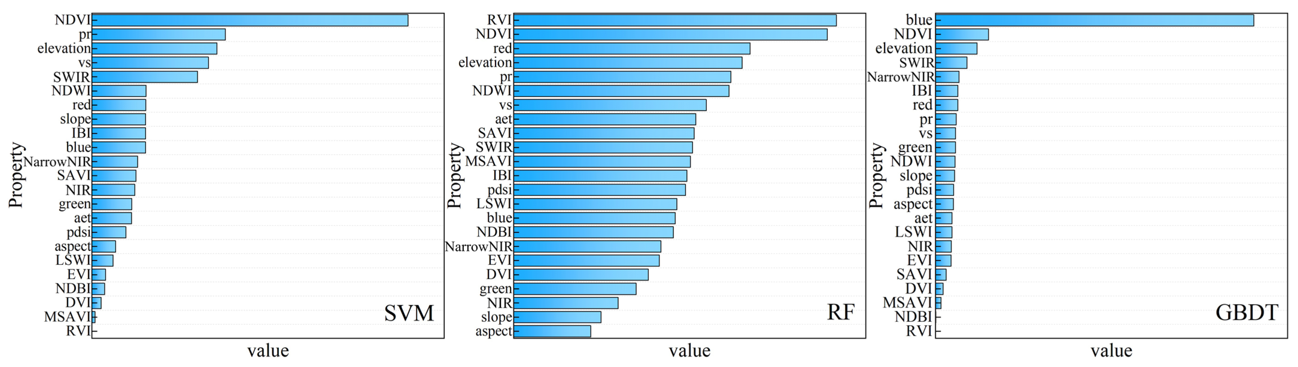
2.3.3. Feature Importance Analysis

In this study, the importance analysis algorithm of the GEE platform was directly invoked to analyze the importance of each feature factor to the inversion model. This algorithm calculates the reduced impurity value of the node according to the probability of the variable feature reaching the node. The node probability can be calculated by dividing the number of samples reaching the node by the total number of samples. The higher the value, the more important the feature is. For each decision tree, the Gini Index is used to calculate the importance of the module nodes, and finally, the relative importance of the feature variables is obtained.
The Gini Index, which indicates the probability that a randomly selected sample in the sample set is misclassified, is used to represent the purity of a dataset. The formula is as follows:
G i n i = k = 1 k p k 1 p k = 1 k = 1 k ( p k ) 2
where: p k represents the probability that the selected sample belongs to the k t h category. The smaller the Gini Index, the smaller the probability of misclassification of selected samples in the dataset, that is, the higher the purity of the dataset.

2.3.4. Accuracy Evaluation

In this study, root mean square error (RMSE) and determination coefficient (R2) were utilized to evaluate the accuracy of the model inversion. The specific calculation formulas are as follows [2]:
R 2 = 1 i = 1 n ( S i S i ) 2 i = 1 n ( S i S i _ ) 2
RMSE   = 1 n i = 1 n ( S i S i ) 2
where: n represents the number of samples, S i represents the measured value of the site, S i represents the predicted value of the model, S i _ represents the average value of the predicted value of the model. In general, the higher the R2 value, the smaller the RMSE value, indicating better model performance.

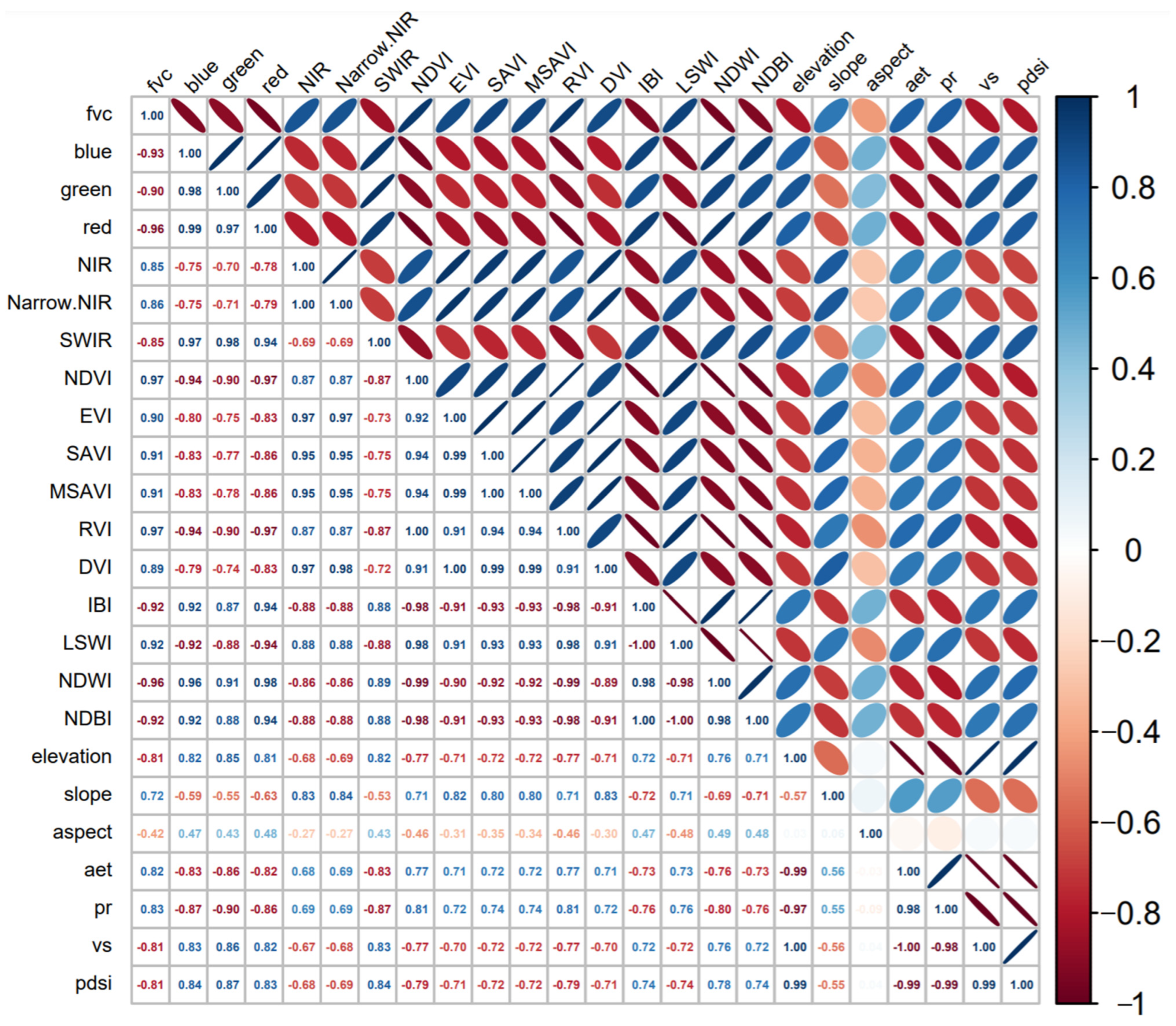
2.3.5. Correlation Analysis of Feature Variables

Exploring the correlation (r) between feature factors and FVC can lead to important feature factors related to vegetation growth change and cover, which is helpful to improve the accuracy of FVC estimation.
r x y = i = 1 n ( x i x ¯ ) ( y i y ¯ ) i = 1 n ( x i x ¯ ) ) 2 i = 1 n ( y i y ¯ ) ) 2
where: r x y is the correlation coefficient between two variables x and y , and the result of the correlation coefficient is between [−1, 1]. x i and y i are the i t h value of x and y variables respectively, x ¯ and y ¯ are the average values of x and y respectively, and n is the number of samples.

2.4. Alpine Grassland Dynamic Simulation Monitoring Methods

The main methods used in dynamic simulation monitoring of alpine grassland were the Theil-Sen slope estimation analysis (Sen’s) and the Mann-Kendall (MK) test. Theil-Sen slope analysis is a robust non-parametric statistical trend calculation method. Sen’s estimation calculates the slope between two data in a time series by taking the median of the slopes as the overall trend of the time series. This method is computationally efficient, insensitive to measured error points and discrete points, and has good stability. It is often used in the analysis of long-term time series data, and its calculation formula is as follows [39]:
β = m e a n X j X i   j i ,   ( 2017     j < i     2022 )
where: x i and x j are the pixel values of remote sensing products in years i and j . M and N are the starting and ending years respectively. β < 0 indicates a decreasing trend, β > 0 indicates an increasing trend.
The Mann-Kendall (MK) test is a non-parametric test method that is usually used to test the significance of time series data as a supplement to Sen’s slope. The principle is to compare the values of the time series over time to determine if a trend exists. The method is based on the rank of the data rather than the original data value, which makes it highly robust to outliers as well, and the independent variables do not need to follow a normal distribution, nor does it require a linear trend, and it is unaffected by missing values and outliers. It has been widely used in the trend significance test of long-term time series data, and is often used in the change trend analysis of precipitation, temperature, runoff, and other time series [40,41]. The MK test method is formulated as follows:
S = i = 1 n 1 j = i + 1 n s g n ( X j X i )
s g n ( X j X i ) = β > 0   1 ,   X j X i   > 0 0 ,   X j X i   = 0 1 ,   X j X i < 0
v a r ( S ) = n ( n 1 ) ( 2 n + 5 ) 18
Z = S / v a r ( S ) ,   S > 0 0 ,   S = 0 ( S + 1 ) / v a r ( S ) ,   S < 0
where: X i and X j are the i and j year FVC data, n is the period length from i to j years, and Z is the standardized test statistic. Z 1 α / 2 is the value corresponding to the confidence level α . This study adopts the confidence level of α = 0.05 and α = 0.01 , corresponding Z 1 α / 2 value of 1.96 and 2.58. When Z > 1.96 and Z > 2.58 , it indicates that the trend passes the significance test with the straightness level of 0.05 and 0.01, respectively. Based on β value and Z value, this study assigns seven grades to the change trend of all remote sensing product values (Table 3). Pixels are marked with extremely significant increase when significance level α = 0.01 and slope β 0.0005 (extremely significant decrease when β 0.0005 ), and with significant increase when significance level α = 0.05 and slope β 0.0005 (significant decrease when β 0.0005 ). Pixels that did not pass the α = 0.05 significance level were labeled with a slight increase ( β 0.0005 ), a slight decrease ( β 0.0005 ), and no significant change (−0.0005 < β < 0.0005), respectively.

3. Results

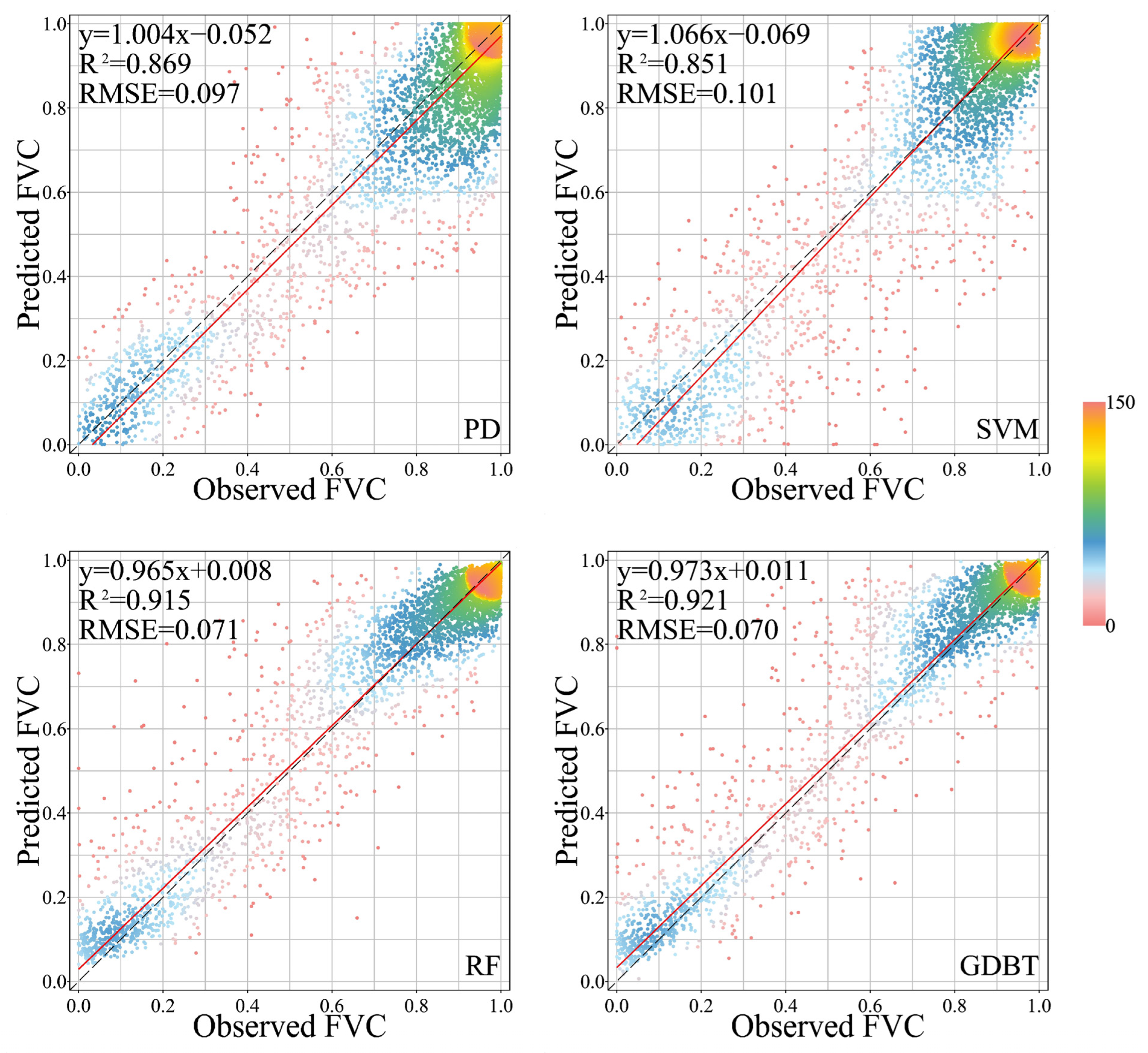
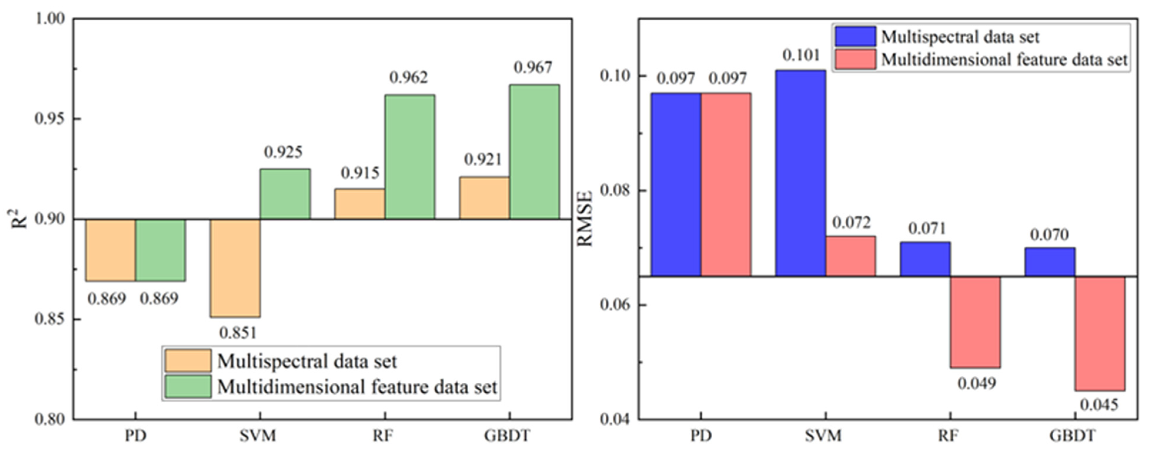
3.1. Model Accuracy Results Based on Sentinel-2 Multispectral Reflectance Dataset

Among the FVC inversion models based on multispectral reflectance data as the driving feature (Figure 5), the accuracy of the GBDT model ( R 2 = 0.921, RMSE = 0.070) was the highest, followed by the RF model accuracy ( R 2 = 0.915, RMSE = 0.071) and the PD model accuracy ( R 2 = 0.869, RMSE = 0.097), and finally the SVM algorithm model ( R 2 = 0.851, RMSE = 0.101).

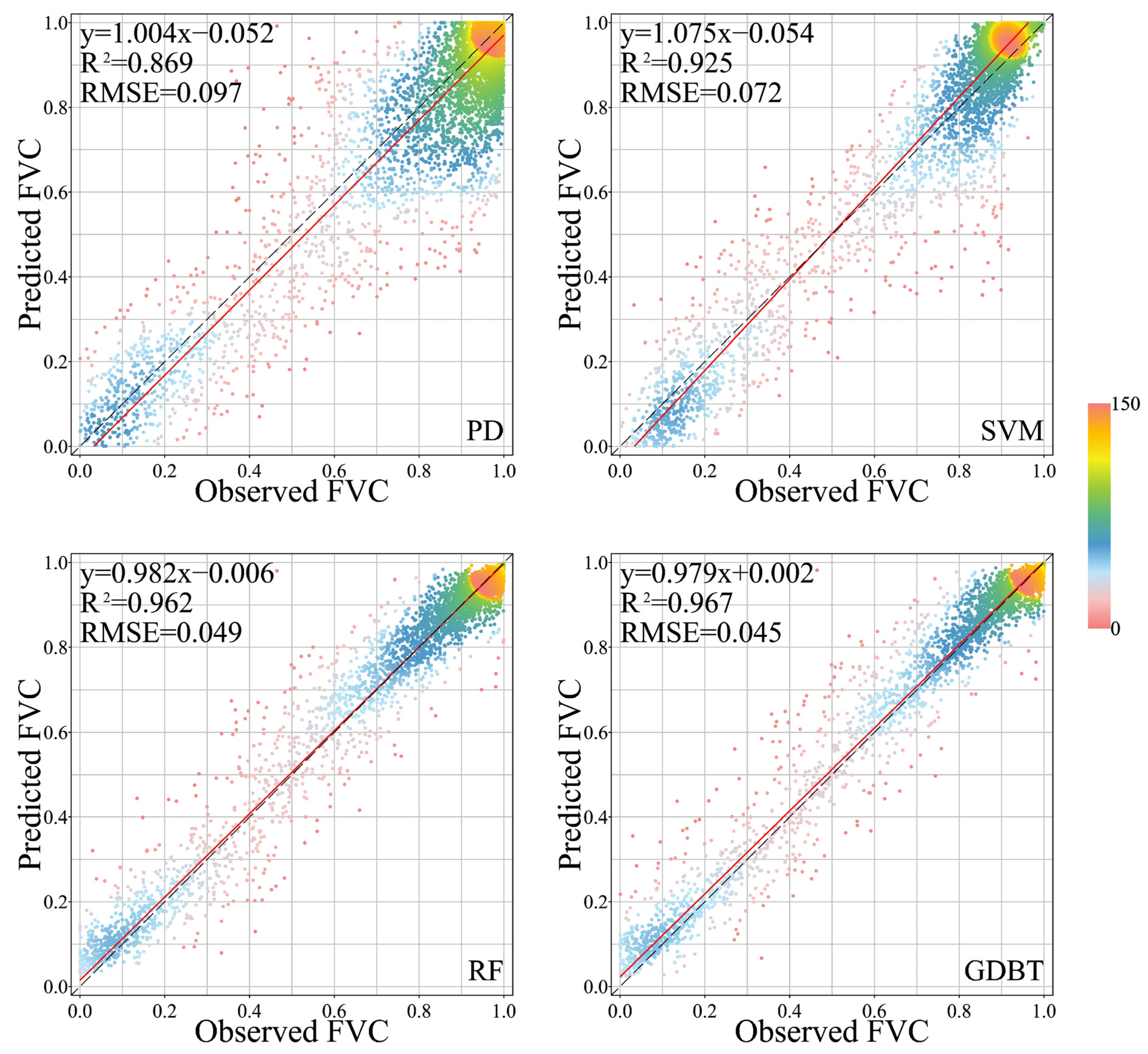
3.2. Model Accuracy Results Based on Sentinel-2 Multidimensional Feature Dataset

When the driving data of FVC inversion is multidimensional feature data (Figure 6), the GBDT model also has the highest accuracy ( R 2 = 0.967, RMSE = 0.045), which is better than the RF model ( R 2 = 0.962, RMSE = 0.049) and the SVM model ( R 2 = 0.925, RMSE = 0.072), and the PD model ( R 2 = 0.869, RMSE = 0.097). When multidimensional feature datasets were used as the driving data for the inversion of the FVC, the inversion model accuracy was higher than that based on multispectral reflectance as the driving data, where the validation accuracy R2 (RMSE) of the SVM, RF, and GBDT inversion results increases (decreases) by 7.4% (2.9%), 4.7% (2.2%), and 4.6% (2.5%), respectively (Figure 7).
The results of the evaluation of the importance of each feature factor in the algorithms show that (Figure 8): In the GBDT model, blue band, NDVI, and elevation are the first three most important driving factors, and the importance of SWIR band and Narrow NIR band driving factors decreases successively. In the RF model, RVI, NDVI, and the red band are the three most important driving factors, and the importance of elevation and precipitation decreases successively. In the SVM model, NDVI, precipitation, and elevation are the top three important factors, followed by wind speed and the SWIR band, and their importance decreases in turn. The top five most important features in these three models all have NDVI and elevation features, indicating that in the algorithm model of this study, these two factors have a vital impact on the accuracy of the inversion results.
The results of the correlation analysis of multiple characterization factors with FVC show that (Figure 9): Within the spectral band, the red band, the blue band, and the green band have an extremely strong correlation with FVC, and the correlations decreased successively, while the NIR band, the Narrow NIR band, and the SWIR have a strong correlation with FVC, and the blue band, the green band, the red band, and the SWIR band have a negative correlation with FVC, whereas the NIR band and Narrow NIR band have a positive correlation with FVC. Among the indices, NDVI, RVI, and NDWI were highly extremely strongly correlated with FVC, while IBI, LSWI, NDBI, MSAVI, SAVI, and EVI were all extremely strongly correlated with FVC, but the correlations decreased successively. DVI is strong correlation with FVC. NDVI, EVI, SAVI, MSAVI, RVI, DVI, LSWI were positively correlated with FVC, while IBI, NDWI, and NDBI were negatively correlated with FVC. Among topographic and climate factors, elevation, slope, aet, pr, vs, pdsi are strongly correlated with FVC, while aspect is moderately correlated with FVC. Among them, aet, pr and slope are positively correlated with FVC. vs, pdsi, elevation, and aspect are negatively correlated with FVC.

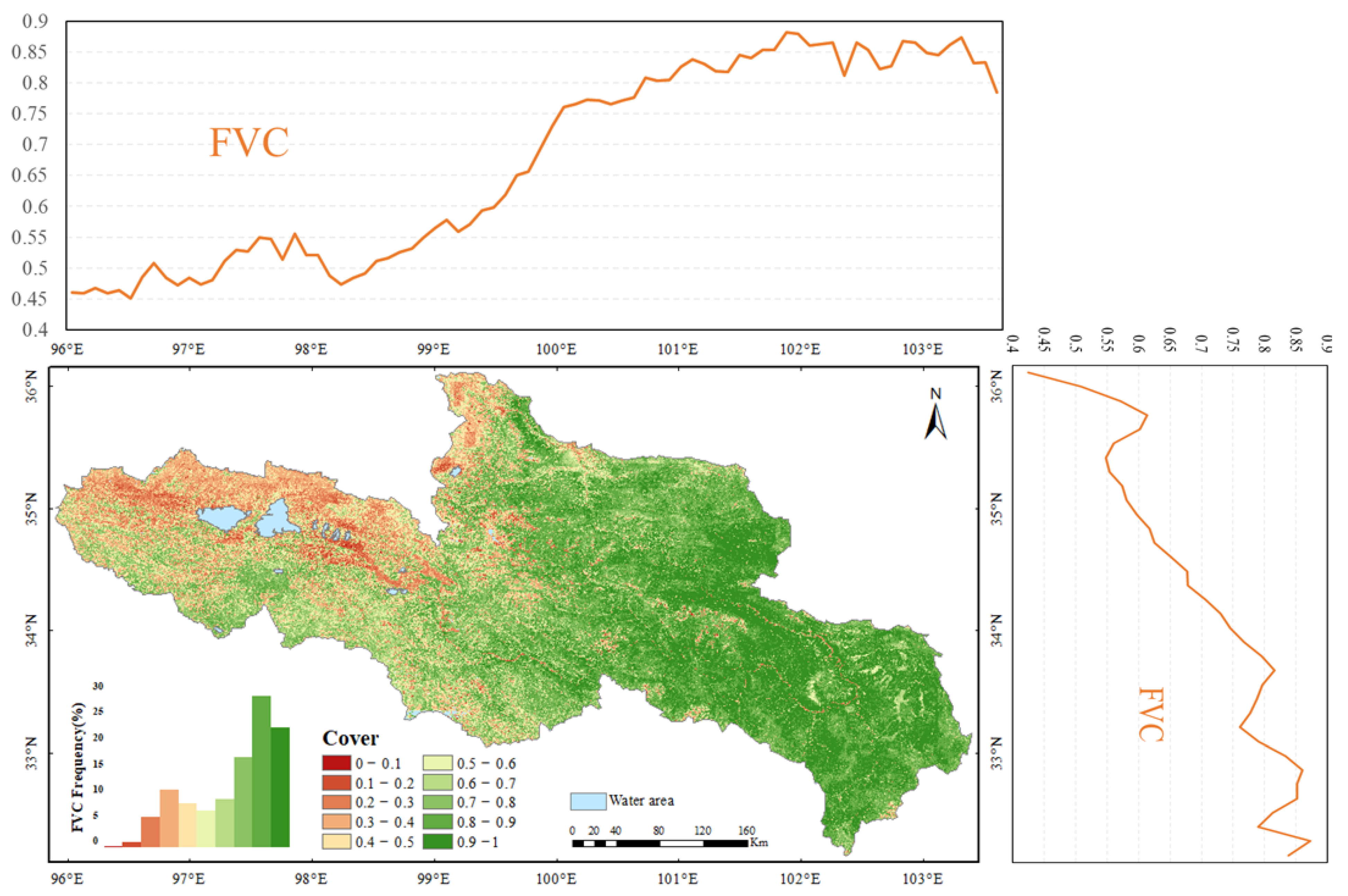
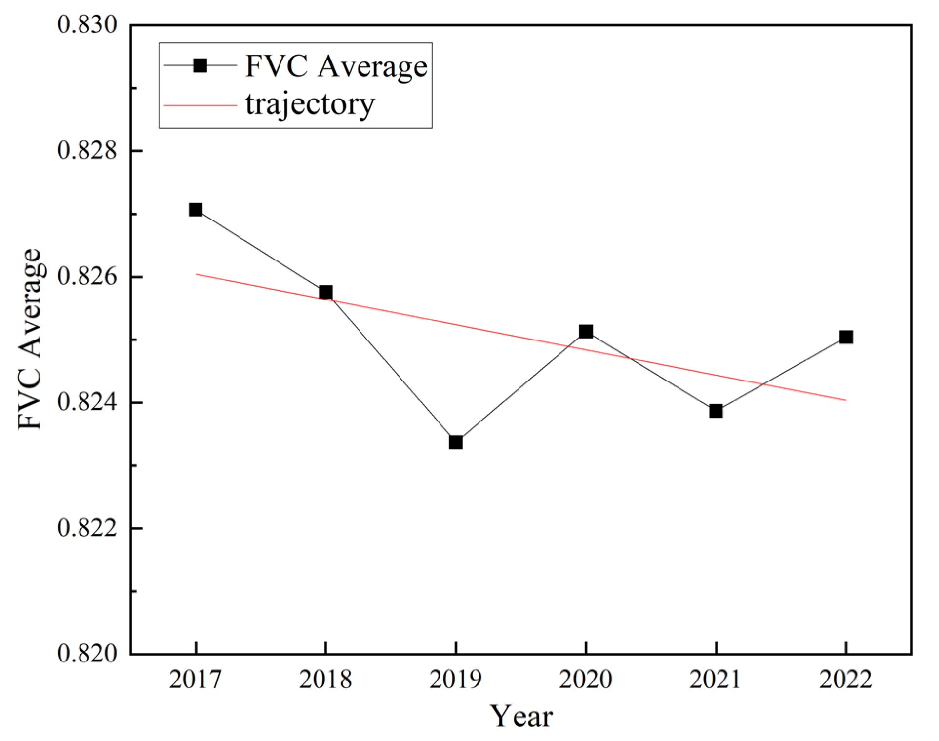
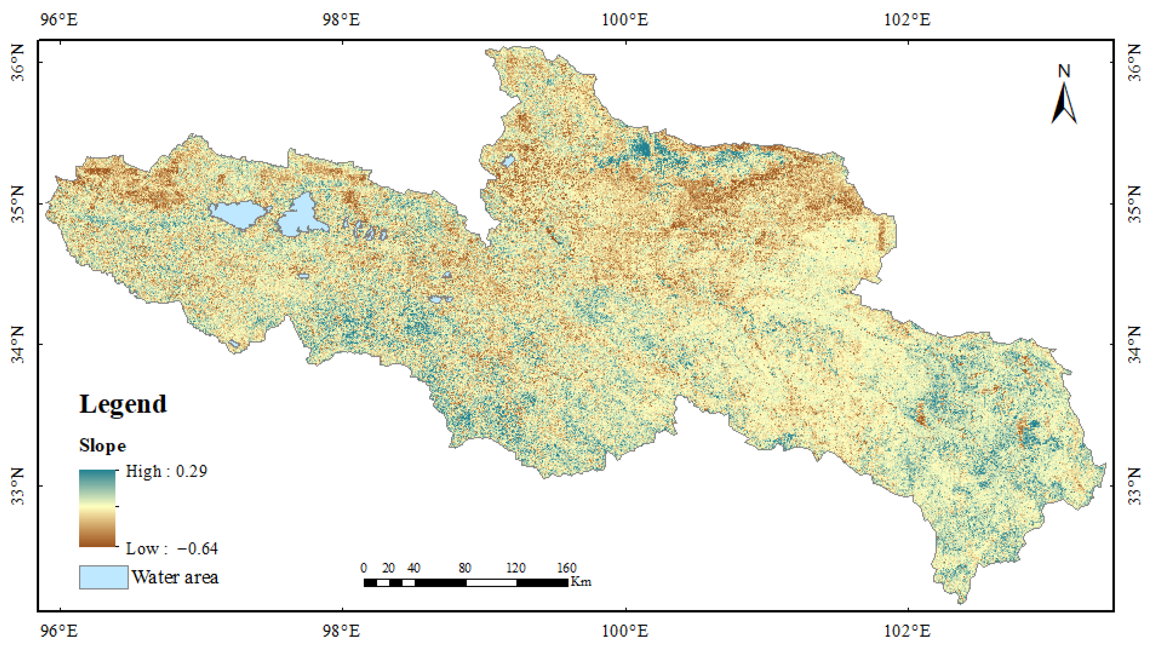
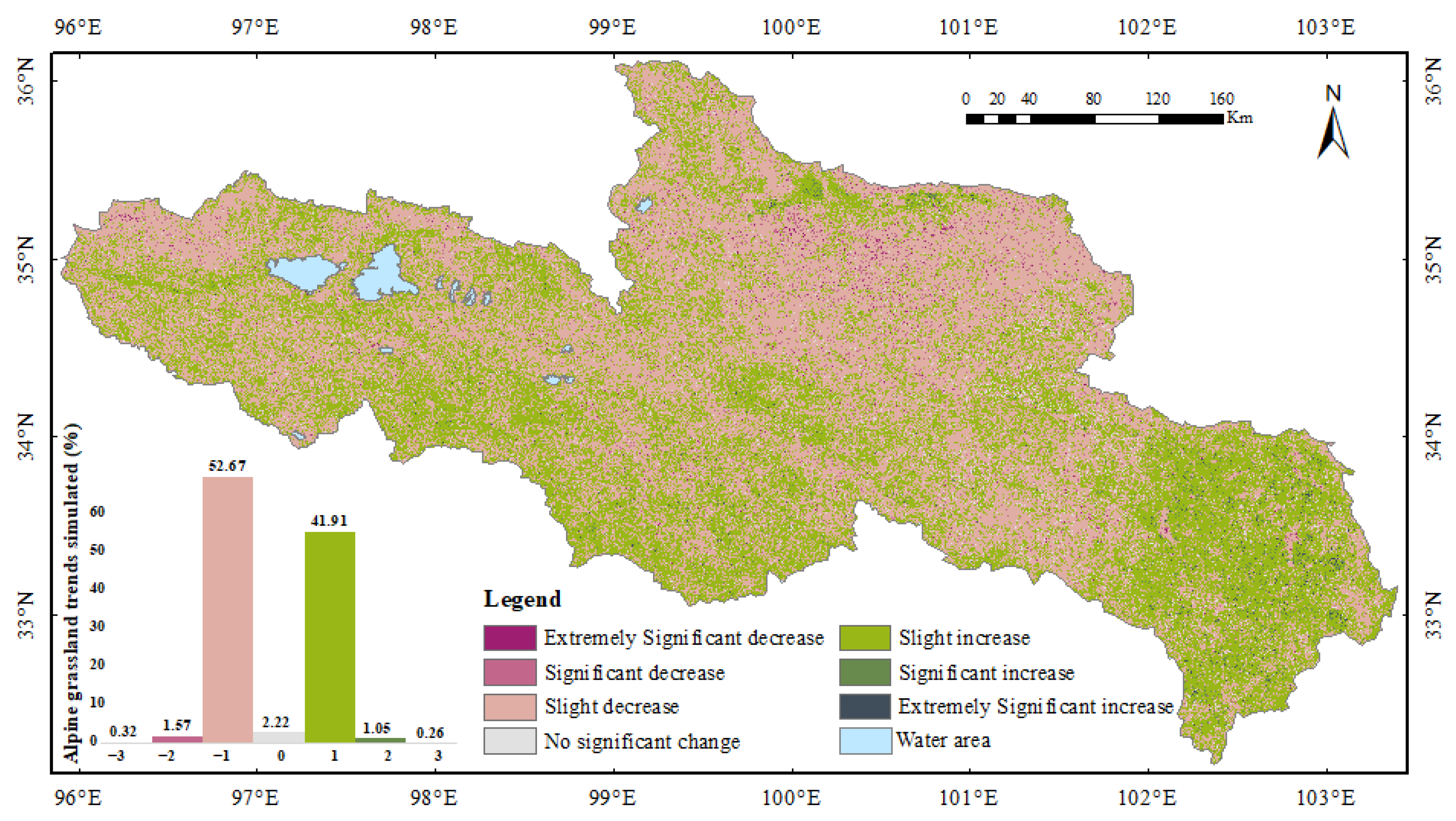
3.3. Spatial Distribution and Trajectory Analysis of FVC in the SRYR

The average spatial distribution data of FVC in the SRYR from 2017 to 2022 (obtained by GBDT model inversion based on a multidimensional feature dataset) show that areas with high FVC were mainly concentrated in the southeast of the study area, while areas with low FVC were mainly concentrated in the northwest of the study area (Figure 10). The FVC values in the northwest are concentrated between 0.2 and 0.5, and those in the southeast are concentrated between 0.7 and 1.0. FVC decreased with increasing latitude and increased with increasing longitude.
During 2017~2022, the average FVC in the whole SRYR fluctuated slightly, ranging from 0.823 to 0.827 (Figure 11). The spatial distribution map of the changes in FVC in the SRYR from 2017 to 2022 (Figure 12) shows that the trajectories slope of change in the study area ranges from −0.64 to 0.29. However, trajectory simulation of alpine grassland in the SRYR (Figure 13) shows that the slope of change of FVC in most regions is small, and the regions with decreasing FVC are mainly distributed in the northwest and north, while the areas with increasing FVC are mainly distributed in the south and southeast. The region characterized by a decreasing trajectory in FVC accounted for 1.89% of the total area, primarily concentrated in the central portion of the study area. Conversely, the area exhibiting an increasing trajectory in FVC constituted 1.31% of the total area, predominantly situated in the southeastern part of the study area.

4. Discussion

4.1. Comparison of Vegetation Coverage Inversion Methods

The PD model is simple, better interpretable, and can quickly simulate the dynamic change of FVC over long time series. However, the selection of endmembers is critical to the success of the PD model [42]. At present, it is a common method to obtain pure vegetation and non-vegetation endmembers by counting the pixel values of the vegetation index and then setting confidence intervals. Therefore, our study used confidence intervals to extract pure vegetation and non-vegetation endmembers from remote sensing images. Our study results show that the accuracy of the PD model is lower than that of the machine learning algorithms, which is similar to the previous research results on the Tibetan Plateau [3,12]. Ge et al. [12] found that the MODIS-based PD model is not applicable to estimate FVC in the Tibetan Plateau region because of the limitation of insufficiently measured pure endmember data matched with image elements. In addition, Lehnert L W et al. [3] found that due to the special situation of the Qinghai-Tibet Plateau, such as high wind speed and bad weather, it is difficult to obtain high-quality field measured spectral data, resulting in a large difference between the measured data and the satellite remote sensing spectral information, thus affecting the training dataset. Therefore, it is difficult to obtain high quality pure vegetation and non-vegetation endmembers in the Tibetan Plateau region, which may be the reason for the low accuracy of PD in the SRYR.
It is a common strategy for remote sensing inversion to invert FVC using multispectral reflectance information from remote sensing images. However, it ignores the influence of other factors on inversion results, and the same vegetation index may be significantly different in different vegetation types [12,43]. Therefore, in the inversion estimation of FVC, it may be more reasonable to construct a multidimensional feature dataset by adding environment factors to the driving dataset. In this study, we compared the machine learning inversion algorithms based on the multispectral reflectance dataset and those based on the multidimensional feature dataset and found that the machine learning models based on the multidimensional feature dataset were generally superior to those based on the multispectral reflectance dataset, in which the validation accuracy R2 (RMSE) of the inversion results of the SVM, RF, and GBDT was increased (decreased) by 7.4% (2.9%), 4.7% (2.2%), and 4.6% (2.5%), respectively. Our research results confirm that the multidimensional feature dataset contributes to the improvement of inversion model accuracy and should be applied in future FVC inversions.
In this study, the GBDT model is superior to the RF model and the SVM model. This is because the GBDT model will evaluate the results of the previous training, update the weight of the driving features on the model during the training process, make the weight of the training features with a large learning error rate in the previous training higher, reduce the residual, and iterate many times in order to obtain the optimal training model. While the RF model takes the average values of multiple decision trees, the SVM model takes the maximum and minimum values according to the characteristics. These two models are all easy to receive outlier interference, so the accuracy of the model is not as stable as GBDT. In addition, other scholars also found that the accuracy of the GBDT model is superior to other machine learning algorithm models. For example, Yang et al. [44] found that GBDT is superior to RF and SVM in crop identification using machine learning algorithms. Ajay Kumar Maurya et al. [45] found that the GBDT algorithm had the best inversion accuracy when using machine learning algorithms to invert FVC based on SAR. Zhang et al. [46] confirmed that GBDT performs better than RF and SVM algorithms from the perspective of model algorithms. Therefore, the GBDT algorithm should be applied to FVC inversion in the future.
In addition, many studies have shown that eXtreme Gradient Boosting (XGBoost) has a wide range of applications in remote sensing index inversion [47,48]. Compared with GBDT, XGBoost introduces specific regularization terms to govern model complexity, thereby enhancing overall generalization capability. A distinctive feature of XGBoost is its automatic utilization of CPU multithreading for parallel operations, a facet that expedites both model training and inference processes [47,48]. However, XGBoost may not perform well in deal with high-dimensional feature data. GBDT is characterized by its flexibility in processing diverse data types and high-dimensional data, coupled with high predictive accuracy. It benefits from robust loss functions like huber, which effectively manage outliers. Due to our study uses high-dimensional data, so we believe that GBDT may be more suitable for our study. Therefore, it’s essential to commend the merit of our chosen approach and may bring some reference value to similar inversions.

4.2. Impact of Drivers on the Accuracy of FVC Inversion

The choice of vegetation index is an important aspect that affects the accuracy of FVC inversion. Vegetation indices such as NDVI, EVI, SAVI, MSAVI, RVI, and DVI can explain the physical characteristics of FVC inversion to a certain extent [1]. NDVI is an important feature factor for the machine learning algorithm models in this study. NDVI can reflect the background influence of vegetation canopy [2,42,49], Our research results are consistent with the results confirmed by other scholars that it has a strong positive correlation with FVC and scores high in machine learning inversion algorithm importance rating. While previous studies have highlighted the sensitivity of vegetation indices such as EVI, SAVI, and MSAVI to soil background, showcasing their capacity to mitigate atmospheric and soil background interference in vegetation information extraction, RVI emerges as more adept at capturing nuanced vegetation growth changes, which demonstrates an ability to detect subtle shifts in vegetation dynamics [42,50,51]. This were also reflected in our study, these indices showed high correlations with FVC and high ratings in the importance ratings. Notwithstanding their valuable insights, vegetation indices have their limitations and uncertainties. To address these, we introduced additional indices like LSWI, NDWI, IBI, and NDBI. Earlier investigations have revealed NDWI’s competence in differentiating between clouds and snow, reducing their influence on FVC inversion outcomes and augmenting accuracy [51]. LSWI monitors vegetation according to the absorption characteristics of vegetation water in the infrared band [52,53]. However, in our study, the importance of NDWI, LSWI are not obvious, probably because the local vegetation water content is low [54,55]. This enhancement is particularly pronounced in plateau regions where unique topography and climate pose FVC calculation challenges. Similarly, our study underscores the utility of NDWI and LSWI in refining FVC calculations in these settings, as evidenced by robust correlations between NDWI, LSWI, and FVC. Furthermore, our findings confirm the efficacy of IBI and NDBI [56,57] in elevating FVC inversion precision in areas with limited vegetation cover, such as urban and human-intensive zones. This underscores the importance of a comprehensive approach considering diverse influencing factors in future FVC inversion research. By incorporating a range of indices tailored to distinct conditions, we enhance the accuracy and reliability of FVC estimations across various landscapes.
Elevation is also an important feature factor in the machine learning models of this study, because the change in altitude will directly affect temperature, precipitation, solar radiation, and other factors closely related to vegetation growth. In the experiment of correlation analysis, we also got confirmation that elevation has a strong correlation with vegetation indices such as NDVI, EVI, SAVI, etc., which are all more than 0.70. The inversion model of alpine FVC can be enhanced by introducing elevation and topography factors, as confirmed in the studies of Liang et al. [58] and Lin et al. [2]. Therefore, topographic features should be considered in the FVC inversion model in the alpine region.
The blue band is the most important characteristic factor in the GBDT model. Probably because the blue band is closely related to the spectral characteristics and physiological structure of vegetation, etc. Healthy vegetation has a strong absorption in the blue and red bands, the blue band played an important role in identifying terrestrial species and subdividing vegetation types due to the influence of chlorophyll and carotenoid absorption [59]. This also coincides with the studies of Trisakti et al. [60] and Hennessy et al. [61]. Especially in the SRYR, where spatial heterogeneity is large and the spectral response of background soil and rock tends to cause large measurement errors [62]. The introduction of the blue band might reduce the model error.

4.3. Analysis of Distribution Characteristics and Changing Trajectories of FVC in the SRYR

The FVC in the SRYR has a trajectory of highs in the east and lows in the west. The high FVC is mainly concentrated in the southeast of the study area, which may be due to the lower elevation, higher temperature, and abundant precipitation in the eastern region, which are favorable to the growth of vegetation [12]. While in the northwestern part of the study area, influenced by elevation, temperature, and precipitation, the overall phenomenon of lower FVC was observed. The spatial distribution of FVC has a similar spatial consistency with the trajectories of annual precipitation, air temperature, and gradually rising elevation from east to west [12]. Overall, it is reasonable that the annual maximum value of FVC in the SRYR shows a trajectory of gradual increase in spatial distribution from west to east and from north to south.
This study uncovers a noteworthy pattern, indicating that the variations in FVC within the SRYR have demonstrated a trajectory of stabilization over the past six years (2017–2022). Others’ studies found that FVC showed an increasing trend in 2000 to 2016 in the Qinghai-Tibet Plateau [12,63], which they suggest may be influenced by the warming and humidification trend on the Tibetan Plateau. However, the significant changes in FVC brought about by these factors were not reflected in our study. In addition, since our study had only 6 years of temporal variation with a short monitoring timescale, this may have resulted in our observation period coinciding with a plateau in the vegetation growth cycle, preventing us from observing an upward trend in vegetation growth or a significant change in vegetation growth dynamics.

5. Conclusions

In this study, based on the FVC data of alpine grassland measured by UAV in 2019 and Sentinel-2 satellite images, we assessed the accuracy of four FVC inversion models, analyzed the influence of the introduction of multidimensional feature factors on the inversion results, and revealed the characteristics of the spatial and temporal changes of the FVC of alpine grassland in the SRYR from 2017 to 2022. The following are the primary conclusions:
The GBDT model is superior to the RF, SVM, and PD models. The inversion model based on a multidimensional feature dataset is superior to that based on a multispectral reflectance dataset. NDVI and elevation play an important role in machine learning inversion algorithms. From 2017 to 2022, the FVC in the SRYR increased gradually from west to east and from north to south, and the decrease trajectories of the FVC in the area were greater than the increase trajectories (54.56% vs. 43.22%), in which most of the grasslands had insignificant trajectories in the change of the FVC, and the areas of significant increase were mainly distributed in the southeast (accounting for 1.31%), and the areas of significant decrease were mainly distributed in the center and northwest (1.89%).

Author Contributions

Conceptualization, G.Z. (Guangrui Zhong) and J.C.; methodology, G.Z. (Guangrui Zhong).; software, G.Z. (Guangrui Zhong); validation, G.Z. (Guangrui Zhong) and J.C.; formal analysis, G.Z. (Guangrui Zhong) and J.C.; investigation, J.C. and R.H.; resources, S.Y. and Y.Q.; data curation, J.C., S.Y. and Y.Q.; writing—original draft preparation, G.Z. (Guangrui Zhong) and J.C.; writing—review and editing, G.Z. (Guangrui Zhong) and J.C.; visualization, H.Y. and X.H.; supervision, S.Y. and G.Z. (Guoqing Zhou); project administration, S.Y.; funding acquisition, J.C. and G.Z. (Guoqing Zhou) All authors have read and agreed to the published version of the manuscript.

Funding

This study was supported by grants from the National Natural Science Foundation of China (42071056, 42361023, 42071139), Guangxi Key Laboratory of Spatial Information and Geomatics (19-050-11-22), and Research Foundation of Guilin University of Technology (GUTQDJJ2017069).

Data Availability Statement

The remotely sensed data and field measured data used in this study is available upon the approval of Jianjun Chen from College of Geomatics and Geoinformation, Guilin University of Technology, Guilin, China.

Conflicts of Interest

The authors declare that they have no known competing financial interests or personal relationships that could have appeared to influence the work reported in this paper.

References

  1. Gao, L.; Wang, X.; Johnson, B.A.; Tian, Q.; Wang, Y.; Verrelst, J.; Mu, X.; Gu, X. Remote sensing algorithms for estimation of fractional vegetation cover using pure vegetation index values: A review. ISPRS J. Photogramm. Remote Sens. 2020, 159, 364–377. [Google Scholar] [CrossRef]
  2. Lin, X.; Chen, J.; Lou, P.; Yi, S.; Qin, Y.; You, H.; Han, X. Improving the estimation of alpine grassland fractional vegetation cover using optimized algorithms and multi-dimensional features. Plant Methods 2021, 17, 96. [Google Scholar] [CrossRef]
  3. Lehnert, L.W.; Meyer, H.; Wang, Y.; Miehe, G.; Thies, B.; Reudenbach, C.; Bendix, J. Retrieval of grassland plant coverage on the Tibetan Plateau based on a multi-scale, multi-sensor and multi-method approach. Remote Sens. Environ. 2015, 164, 197–207. [Google Scholar] [CrossRef]
  4. Wang, B.J.; Liang, S.; Xie, X.; Wei, X.; Zhao, X.; Yao, Y.; Zhang, X. Assessment of Sentinel-2 MSI Spectral Band Reflectances for Estimating Fractional Vegetation Cover. Remote Sens. 2018, 10, 1927. [Google Scholar] [CrossRef]
  5. Liu, D.; Jia, K.; Xia, M.; Wei, X.; Yao, Y.; Zhang, X.; Tao, G. Fractional Vegetation Cover Estimation Algorithm Based on Recurrent Neural Network for MODIS 250 m Reflectance Data. IEEE J. Sel. Top. Appl. Earth Obs. Remote Sens. 2021, 14, 6532–6543. [Google Scholar] [CrossRef]
  6. Su, L. Optimizing support vector machine learning for semi-arid vegetation mapping by using clustering analysis. ISPRS J. Photogramm. Remote Sens. 2009, 64, 407–413. [Google Scholar] [CrossRef]
  7. Hansen, M.C.; DeFries, R.S.; Townshend, J.R.G.; Carroll, M.; Dimiceli, C.; Sohlberg, R.A. Global Percent Tree Cover at a Spatial Resolution of 500 Meters: First Results of the MODIS Vegetation Continuous Fields Algorithm. Earth Interact. 2003, 7, 1–15. [Google Scholar] [CrossRef]
  8. Fuster, B.; Sánchez-Zapero, J.; Camacho, F.; García-Santos, V.; Verger, A.; Lacaze, R.; Weiss, M.; Baret, F.; Smets, B. Quality Assessment of PROBA-V LAI, fAPAR and fCOVER Collection 300 m Products of Copernicus Global Land Service. Remote Sens. 2020, 12, 1017. [Google Scholar] [CrossRef]
  9. Xiao, Z.; Liang, S.; Sun, R.; Wang, J.; Jiang, B. Estimating the fraction of absorbed photosynthetically active radiation from the MODIS data based GLASS leaf area index product. Remote Sens. Environ. 2015, 171, 105–117. [Google Scholar] [CrossRef]
  10. Xiao, Z.; Liang, S.; Sun, R. Evaluation of Three Long Time Series for Global Fraction of Absorbed Photosynthetically Active Radiation (FAPAR) Products. IEEE Trans. Geosci. Remote Sens. 2018, 56, 5509–5524. [Google Scholar] [CrossRef]
  11. Zhao, J.; Li, J.; Liu, Q.; Xu, B.; Yu, W.; Lin, S.; Hu, Z. Estimating fractional vegetation cover from leaf area index and clumping index based on the gap probability theory. Int. J. Appl. Earth Obs. Geoinf. 2020, 90, 102112. [Google Scholar] [CrossRef]
  12. Ge, J.; Meng, B.; Liang, T.; Feng, Q.; Gao, J.; Yang, S.; Huang, X.; Xie, H. Modeling alpine grassland cover based on MODIS data and support vector machine regression in the headwater region of the Huanghe River, China. Remote Sens. Environ. 2018, 218, 162–173. [Google Scholar] [CrossRef]
  13. Yang, L.J.; Liang, S.; Liu, J.; Wang, X. Comparison of Four Machine Learning Methods for Generating the GLASS Fractional Vegetation Cover Product from MODIS Data. Remote Sens. 2016, 8, 682. [Google Scholar] [CrossRef]
  14. Huang, R.; Chen, J.; Feng, Z.; Yang, Y.; You, H.; Han, X. Fitness for Purpose of Several Fractional Vegetation Cover Products on Monitoring Vegetation Cover Dynamic Change—A Case Study of an Alpine Grassland Ecosystem. Remote Sens. 2023, 15, 1312. [Google Scholar] [CrossRef]
  15. Hao, F.; Zhang, X.; Ouyang, W.; Skidmore, A.K.; Toxopeus, A.G. Vegetation NDVI Linked to Temperature and Precipitation in the Upper Catchments of Yellow River. Environ. Model. Assess. 2011, 17, 389–398. [Google Scholar] [CrossRef]
  16. Zhang, Z.; Dong, X.; Tian, J.; Tian, Q.; Xi, Y.; He, D. Stand density estimation based on fractional vegetation coverage from Sentinel-2 satellite imagery. Int. J. Appl. Earth Obs. Geoinf. 2022, 108, 102760. [Google Scholar] [CrossRef]
  17. Cai, Y.; Zhang, M.; Lin, H. Estimating the Urban Fractional Vegetation Cover Using an Object-Based Mixture Analysis Method and Sentinel-2 MSI Imagery. IEEE J. Sel. Top. Appl. Earth Obs. Remote Sens. 2020, 13, 341–350. [Google Scholar] [CrossRef]
  18. Yu, R.; Li, S.; Zhang, B.; Zhang, H. A deep transfer learning method for estimating fractional vegetation cover of sentinel-2 multispectral images. IEEE Geosci. Remote Sens. Lett. 2021, 19, 1–5. [Google Scholar] [CrossRef]
  19. Chen, J.; Zhao, X.; Zhang, H.; Qin, Y.; Yi, S. Evaluation of the Accuracy of the Field Quadrat Survey of Alpine Grassland Fractional Vegetation Cover Based on the Satellite Remote Sensing Pixel Scale. ISPRS Int. J. Geo-Inf. 2019, 8, 497. [Google Scholar] [CrossRef]
  20. Okin, G.S.; Clarke, K.D.; Lewis, M.M. Comparison of methods for estimation of absolute vegetation and soil fractional cover using MODIS normalized BRDF-adjusted reflectance data. Remote. Sens. Environ. 2013, 130, 266–279. [Google Scholar] [CrossRef]
  21. Chen, J.; Yi, S.; Qin, Y.; Wang, X. Improving estimates of fractional vegetation cover based on UAV in alpine grassland on the Qinghai–Tibetan Plateau. Int. J. Remote Sens. 2016, 37, 1922–1936. [Google Scholar] [CrossRef]
  22. Chen, J.; Chen, Z.; Huang, R.; You, H.; Han, X.; Yue, T.; Zhou, G. The Effects of Spatial Resolution and Resampling on the Classification Accuracy of Wetland Vegetation Species and Ground Objects: A Study Based on High Spatial Resolution UAV Images. Drones 2023, 7, 61. [Google Scholar] [CrossRef]
  23. Yin, F.; Lewis, P.E.; Gomez-Dans, J.L.; Wu, Q. A sensor-invariant atmospheric correction method: Application to Sentinel-2/MSI and Landsat 8/OLI. Geosci. Model Dev. 2022, 15, 7933–7976. [Google Scholar] [CrossRef]
  24. Zhao, Y.; Potgieter, A.B.; Zhang, M.; Wu, B.; Hammer, G.L. Predicting Wheat Yield at the Field Scale by Combining High-Resolution Sentinel-2 Satellite Imagery and Crop Modelling. Remote. Sens. 2020, 12, 1024. [Google Scholar] [CrossRef]
  25. Chandrasekar, K.; Sesha Sai, M.V.R.; Roy, P.S.; Dwevedi, R.S. Land Surface Water Index (LSWI) response to rainfall and NDVI using the MODIS Vegetation Index product. Int. J. Remote Sens. 2010, 31, 3987–4005. [Google Scholar] [CrossRef]
  26. Gao, B.-c. NDWI—A normalized difference water index for remote sensing of vegetation liquid water from space. Remote Sens. Environ. 1996, 58, 257–266. [Google Scholar] [CrossRef]
  27. Rouse, J.W.; Haas, R.H.; Schell, J.A. Monitoring Vegetation Systems in the Great Plains with Erts. NASA Spec. Publ. 1974, 351, 309. [Google Scholar]
  28. Huete, A.; Didan, K.; Miura, T.; Rodriguez, E.P.; Gao, X.; Ferreira, L.G. Overview of the radiometric and biophysical performance of the MODIS vegetation indices. Remote Sens. Environ. 2002, 83, 195–213. [Google Scholar] [CrossRef]
  29. Huete, A.R. A soil-adjusted vegetation index (SAVI). Remote Sens. Environ. 1988, 25, 295–309. [Google Scholar] [CrossRef]
  30. Qi, J.; Chehbouni, A.; Huete, A.R.; Kerr, Y.H.; Sorooshian, S. A modified soil adjusted vegetation index. Remote Sens. Environ. 1994, 48, 119–126. [Google Scholar] [CrossRef]
  31. Birth, G.S.; McVey, G.R. Measuring the Color of Growing Turf with a Reflectance Spectrophotometer. Agron. J. 1968, 60, 640–643. [Google Scholar] [CrossRef]
  32. Jordan, C.F. Derivation of Leaf-Area Index from Quality of Light on the Forest Floor. Ecology 1969, 50, 663–666. [Google Scholar] [CrossRef]
  33. Xu, H. A new index for delineating built-up land features in satellite imagery. Int. J. Remote Sens. 2008, 29, 4269–4276. [Google Scholar] [CrossRef]
  34. Zha, Y.; Ni, S.-x.; Yang, S. An Effective Approach to Automatically Extract Urban Land-use from TM lmagery. J. Remote Sens. 2003, 01, 37–40. [Google Scholar]
  35. Cortes, C.; Vapnik, V. Support-vector networks. Mach. Learn. 1995, 20, 273–297. [Google Scholar] [CrossRef]
  36. Scornet, E. Random Forests and Kernel Methods. IEEE Trans. Inf. Theory 2016, 62, 1485–1500. [Google Scholar] [CrossRef]
  37. Chen, T.; Zhu, L.; Niu, R.-q.; Trinder, C.J.; Peng, L.; Lei, T. Mapping landslide susceptibility at the Three Gorges Reservoir, China, using gradient boosting decision tree, random forest and information value models. J. Mt. Sci. 2020, 17, 670–685. [Google Scholar] [CrossRef]
  38. Sigrist, F. Gradient and Newton boosting for classification and regression. Expert Syst. Appl. 2020, 167, 114080. [Google Scholar] [CrossRef]
  39. Zuo, Y.; Li, Y.; He, K.; Wen, Y. Temporal and Spatial Variation Characteristics of Vegetation Coverage and Quantitative Analysis of Its Potential Driving Forces in the Qilian Mountains, China, 2000–2020. Ecol. Indic. 2022, 143, 109429. [Google Scholar] [CrossRef]
  40. Li, F.F.; Lu, H.L.; Wang, G.Q.; Yao, Z.Y.; Li, Q.; Qiu, J. Zoning of Precipitation Regimes on the Qinghai–Tibet Plateau and Its Surrounding Areas Responded by the Vegetation Distribution. Sci. Total Environ. 2022, 838, 155844. [Google Scholar] [CrossRef]
  41. Yan, X.; Li, J.; Shao, Y.; Hu, Z.; Yang, Z.; Yin, S.; Cui, l. Driving forces of grassland vegetation changes in Chen Barag Banner, Inner Mongolia. GIScience Remote Sens. 2020, 57, 753–769. [Google Scholar] [CrossRef]
  42. Xiao, J.; Moody, A. A comparison of methods for estimating fractional green vegetation cover within a desert-to-upland transition zone in central New Mexico, USA. Remote Sens. Environ. 2005, 98, 237–250. [Google Scholar] [CrossRef]
  43. Liu, D.; Jia, K.; Jiang, H.; Xia, M.; Tao, G.; Wang, B.; Chen, Z.; Yuan, B.; Li, J. Fractional Vegetation Cover Estimation Algorithm for FY-3B Reflectance Data Based on Random Forest Regression Method. Remote Sens. 2021, 13, 2165. [Google Scholar] [CrossRef]
  44. Yang, L.; Mansaray, L.; Huang, J.; Wang, L. Optimal Segmentation Scale Parameter, Feature Subset and Classification Algorithm for Geographic Object-Based Crop Recognition Using Multisource Satellite Imagery. Remote. Sens. 2019, 11, 514. [Google Scholar] [CrossRef]
  45. Maurya, A.K.; Bhargava, N.; Singh, D. Efficient selection of SAR features using ML based algorithms for accurate FVC estimation. Adv. Space Res. 2022, 70, 1795–1809. [Google Scholar] [CrossRef]
  46. Zhang, C.; Liu, C.; Zhang, X.; Almpanidis, G. An up-to-date comparison of state-of-the-art classification algorithms. Expert Syst. Appl. 2017, 82, 128–150. [Google Scholar] [CrossRef]
  47. Wang, N.; Guo, Y.; Wei, X.; Zhou, M.; Wang, H.; Bai, Y. UAV-based remote sensing using visible and multispectral indices for the estimation of vegetation cover in an oasis of a desert. Ecol. Indic. 2022, 141, 109155. [Google Scholar] [CrossRef]
  48. Bartold, M.; Kluczek, M. A Machine Learning Approach for Mapping Chlorophyll Fluorescence at Inland Wetlands. Remote. Sens. 2023, 15, 2392. [Google Scholar] [CrossRef]
  49. Carlson, T.N.; Ripley, D.A. On the relation between NDVI, fractional vegetation cover, and leaf area index. Remote Sens. Environ. 1997, 62, 241–252. [Google Scholar] [CrossRef]
  50. Ayanlade, A. Remote sensing vegetation dynamics analytical methods: A review of vegetation indices techniques. Geoinformatica Pol. 2017, 16, 7–17. [Google Scholar] [CrossRef]
  51. Eswar, R.; Sekhar, M.; Bhattacharya, B.K. Disaggregation of LST over India: Comparative analysis of different vegetation indices. Int. J. Remote Sens. 2016, 37, 1035–1054. [Google Scholar] [CrossRef]
  52. Zheng, J.; Li, F.; Du, X. Using Red Edge Position Shift to Monitor Grassland Grazing Intensity in Inner Mongolia. J. Indian Soc. Remote Sens. 2017, 46, 81–88. [Google Scholar] [CrossRef]
  53. Zhao, B.; Yan, Y.; Guo, H.; He, M.; Gu, Y.; Li, B. Monitoring rapid vegetation succession in estuarine wetland using time series MODIS-based indicators: An application in the Yangtze River Delta area. Ecol. Indic. 2009, 9, 346–356. [Google Scholar] [CrossRef]
  54. Ma, Z.; Wu, B.; Yan, N.; Zhu, W.; Zeng, H.; Xu, J. Spatial Allocation Method from Coarse Evapotranspiration Data to Agricultural Fields by Quantifying Variations in Crop Cover and Soil Moisture. Remote. Sens. 2021, 13, 343. [Google Scholar] [CrossRef]
  55. Cheng, W.; Xi, H.; Sindikubwabo, C.; Si, J.; Zhao, C.; Yu, T.; Li, A.; Wu, T. Ecosystem health assessment of desert nature reserve with entropy weight and fuzzy mathematics methods: A case study of Badain Jaran Desert. Ecol. Indic. 2020, 119, 106843. [Google Scholar] [CrossRef]
  56. Yang, X.; Meng, F.; Fu, P.; Zhang, J.; Liu, Y. Instability of remote sensing ecological index and its optimisation for time frequency and scale. Ecol. Informatics 2022, 72, 101870. [Google Scholar] [CrossRef]
  57. Guo, N.; Liang, X.; Meng, L. Evaluation of the Thermal Environmental Effects of Urban Ecological Networks—A Case Study of Xuzhou City, China. Sustainability 2022, 14, 7744. [Google Scholar] [CrossRef]
  58. Liang, S.; Ge, S.; Wan, L.; Xu, D. Characteristics and causes of vegetation variation in the source regions of the Yellow River, China. Int. J. Remote Sens. 2011, 33, 1529–1542. [Google Scholar] [CrossRef]
  59. Myneni, R.B.; Hall, F.G.; Sellers, P.J.; Marshak, A.L. The interpretation of spectral vegetation indexes. IEEE Trans. Geosci. Remote Sens. 1995, 33, 481–486. [Google Scholar] [CrossRef]
  60. Trisakti, B. Vegetation type classification and vegetation cover percentage estimation in urban green zone using pleiades imagery. IOP Conf. Ser. Earth Environ. Sci. 2017, 54, 012003. [Google Scholar] [CrossRef]
  61. Hennessy, A.; Clarke, K.; Lewis, M. Hyperspectral Classification of Plants: A Review of Waveband Selection Generalisability. Remote Sensing 2020, 12, 113. [Google Scholar] [CrossRef]
  62. Smith, M.O.; Ustin, S.L.; Adams, J.B.; Gillespie, A.R. Vegetation in deserts: I. A regional measure of abundance from multispectral images. Remote Sens. Environ. 1990, 31, 1–26. [Google Scholar] [CrossRef]
  63. Meng, B.; Gao, J.; Liang, T.; Cui, X.; Ge, J.; Yin, J.; Feng, Q.; Xie, H. Modeling of Alpine Grassland Cover Based on Unmanned Aerial Vehicle Technology and Multi-Factor Methods: A Case Study in the East of Tibetan Plateau, China. Remote. Sens. 2018, 10, 320. [Google Scholar] [CrossRef]
Figure 1. Overview of the study area in the SRYR. (a) Location of the study area; (b) Topography of the study area.
Remotesensing 15 04266 g001
Figure 2. UAV route planning and field data acquisition.
Remotesensing 15 04266 g002
Figure 3. Processing of UAV actual aerial image. (a) UAV aerial photography to obtain the coverage image; (b) the red box of (a); (c)the EGI segmentation results of the aerial image; (d) the EGI segmentation results of the red box.
Remotesensing 15 04266 g003
Figure 4. ① The blue box shows the preprocessing process of UAV, Sentinel-2 and other supporting data (climate data, topographic data); ② The green box shows the extracted multidimensional feature dataset; ③ The red box shows the construction of FVC inversion model with multispectral reflectance dataset and FVC inversion model with multidimensional feature dataset; ④ The yellow box shows the acquisition of the spatial distribution of FVC in SRYR and its dynamic changes.
Remotesensing 15 04266 g004
Figure 5. Evaluation of inversion accuracy based on multispectral reflectance dataset by PD model, SVM model, RF model and GBDT model.
Remotesensing 15 04266 g005
Figure 6. Evaluation of inversion accuracy based on multidimensional feature dataset by PD model, SVM model, RF model and GBDT model.
Remotesensing 15 04266 g006
Figure 7. Comparison of inversion model accuracy.
Remotesensing 15 04266 g007
Figure 8. Evaluation of the importance of each feature factor in the algorithms.
Remotesensing 15 04266 g008
Figure 9. Correlation of each feature factor. (Note: The “\” direction is negatively correlated and the “/” direction is positively correlated).
Remotesensing 15 04266 g009
Figure 10. Spatial map of average FVC results in the SRYR from 2017 to 2022. (Note: The line chart is the FVC average corresponding to the spatial distribution.).
Remotesensing 15 04266 g010
Figure 11. Inversion trajectories of the mean FVC in the SRYR from 2017 to 2022.
Remotesensing 15 04266 g011
Figure 12. Change trajectories of grassland coverage in the SRYR from 2017 to 2022.
Remotesensing 15 04266 g012
Figure 13. Trajectory simulation of alpine grassland in the SRYR.
Remotesensing 15 04266 g013
Table 1. The basic information of FVC products.
FVC ProductsSensorsTemporal\Spatial ResolutionTime RangeSpatial RangeProduction Algorithms
GEOV1SPOT-V
PROBA-V
10 d\1 km1999~2014
2014~2020
GlobalNeural network
GEOV2SPOT-V
PROBA-V
10 d\1 km1999~2014
2014~2020
GlobalNeural network
GEOV3PROBA-V
Sentinel-3
10 d\300 m2014~2020
2020~ at present
GlobalNeural network
GLASSAVHRR
MODIS
8 d\500 m1986~2020
1999~2020
GlobalGeneralized Regression Neural network,
Multiple Adaptive Regression Splines
MuSyQMODIS,
VIIRS etc.
4 d\500 m2001~2019GlobalPorosity Algorithm
Note: V is VEGETATION sensors.
Table 2. Calculation method of vegetation index.
IndexCalculation FormulaReference
NDVI N D V I = ( N I R R E D ) / ( N I R + R E D ) Rouse et al. [27]
EVI E V I = 2.5 × ( N I R R E D ) / ( N I R + 6 × R E D 7.5 × B L U E + 1 ) Huete et al. [28]
SAVI S A V I = ( 1 + L ) × ( N I R R E D ) / ( N I R + R E D + L ) Huete et al. [29]
MSAVI M S A V I = [ 2 × N I R + 1 ( 2 × N I R + 1 ) 2 8 × ( N I R R e d )   ] / 2 Qi et al. [30]
RVI R V I = N I R / R e d Birth et al. [31]
DVI D V I = N I R R e d Jordan et al. [32]
IBI I B I = 2 S W I R S W I R + N I R [ N I R N I R + R e d + G r e e n G r e e n + S W I R ] 2 S W I R S W I R + N I R + [ N I R N I R + R e d + G r e e n G r e e n + S W I R ] Xu et al. [33]
LSWI L S W I = ( N I R S W I R ) / ( N I R + S W I R ) Chandrasekar et al. [25]
NDWI N D W I = ( G r e e n N I R ) / ( G r e e n + N I R ) Gao et al. [26]
NDBI N D B I = ( S W I R N I R ) / ( S W I R + N I R ) Zha et al. [34]
Note: L is the soil conditioning factor.
Table 3. Level classification of the FVC value’s change trend.
SlopeConfident Levels Z ValuesChanging Trend
β  0.0005 α = 0.01 Z > 2.58Extremely significant increase
β  0.0005 α = 0.01 Z > 2.58Extremely significant decrease
β  0.0005 α = 0.052.58 Z > 1.96Significant increase
β  0.0005 α = 0.052.58 Z > 1.96Significant decrease
β  0.0005 α = 0.05 Z 1.96 Slightly increase
β  0.0005 α = 0.05 Z 1.96 Slightly decrease
−0.0005 <  β  < 0.0005 α = 0.05 Z 1.96 No significant change
Disclaimer/Publisher’s Note: The statements, opinions and data contained in all publications are solely those of the individual author(s) and contributor(s) and not of MDPI and/or the editor(s). MDPI and/or the editor(s) disclaim responsibility for any injury to people or property resulting from any ideas, methods, instructions or products referred to in the content.

