Article

Fractional Vegetation Cover Estimation Algorithm for FY-3B Reflectance Data Based on Random Forest Regression Method

1
State Key Laboratory of Remote Sensing Science, Faculty of Geographical Science, Beijing Normal University, Beijing 100875, China
2
Beijing Engineering Research Center for Global Land Remote Sensing Products, Faculty of Geographical Science, Beijing Normal University, Beijing 100875, China
*
Author to whom correspondence should be addressed.
Remote Sens. 2021, 13(11), 2165; https://doi.org/10.3390/rs13112165
Submission received: 9 April 2021 / Revised: 23 May 2021 / Accepted: 28 May 2021 / Published: 31 May 2021
(This article belongs to the Special Issue Advances on Land–Ocean Heat Fluxes Using Remote Sensing)

Abstract

:
As an important land surface vegetation parameter, fractional vegetation cover (FVC) has been widely used in many Earth system ecological and climate models. In particular, high-quality and reliable FVC products on the global scale are important for the Earth surface process simulation and global change studies. Recently, the FengYun-3 (FY-3) series satellites, which are the second generation of Chinese meteorological satellites, launched with the polar orbit and provide continuous land surface observations on a global scale. However, there is rare studying on the FVC estimation using FY-3 reflectance data. Therefore, the FY-3B reflectance data were selected as the representative data to develop a FVC estimation algorithm in this study, which would investigate the capability of the FY-3 reflectance data on the global FVC estimation. The spatial–temporal validation over the regional area indicated that the FVC estimations generated by the proposed algorithm had reliable continuities. Furthermore, a satisfactory accuracy performance (R2 = 0.7336, RMSE = 0.1288) was achieved for the proposed algorithm based on the Earth Observation LABoratory (EOLAB) reference FVC data, which provided further evidence on the reliability and robustness of the proposed algorithm. All these results indicated that the FY-3 reflectance data were capable of generating a FVC estimation with reliable spatial–temporal continuities and accuracy.

Graphical Abstract

1. Introduction

Fractional vegetation cover (FVC), defined as the percentage of green vegetation over the total statistical area seen from nadir, is an important biophysical parameter to describe the growth state of land surface vegetation [1,2,3]. High-quality FVC products, particularly over a global scale, are essential for the land surface process models and related researches [4,5,6]. At present, remote sensing technology is capable of acquiring various land surface observations efficiently and has become a feasible way for FVC estimations on the regional and global scales.
Over the past decades, several FVC products have been generated using remote sensing data (Table 1) [7,8]. Among these FVC products, a linear inversion model was built and adopted to generate the POLarization and Directionality of the Earth’s Reflectances of National Centre for Space Studies (CNES/POLDER) FVC product, which was only available for years 1996, 1997, and 2003 [2]. The EUMETSAT Satellite Application Facility on Land Surface Analysis (LSA SAF) FVC product covering Europe, Africa, and South America is generated based on the spectral mixture analysis method [9]. Besides, the Carbon Cycle and Change in Land Observational Products from an Ensemble of Satellites (CYCLOPES) and European Space Agency/Medium Resolution Imaging Spectrometer (ESA/MERIS) FVC products are obtained using the neural network method with the sample data derived from the PROSPECT + SAIL (PROSAIL) canopy radiative transfer model [10,11]. However, the CYCLOPES FVC product shows a systematic underestimation (up to 0.2) in croplands [12], and the MERIS FVC product has no longer been generated since 2012 [13]. The VGT bioGEOphysical (GEOV) series FVC products (including GEOV1, GEOV2, and GEOV3) are generated using the neural network, and the targeted FVC value in training samples are extracted from the CYCLOPES FVC product [1,14,15]. Nevertheless, both the GEOV1 and GEOV3 FVC products present poor performances in spatial–temporal continuities with a large amount of missing data [16]. Besides, there are high uncertainties over the low FVC values of the GEOV2 FVC product [8]. Furthermore, the Global LAnd Surface Satellite (GLASS) FVC product is generated using the Multivariate Adaptive Regression Splines (MARS) and shows reliable spatial–temporal continuities and assessment accuracies [8,17]. However, the GLASS FVC product is obtained from the Moderate Resolution Imaging Spectroradiometer (MODIS) reflectances, and the design lifespan of the MODIS operation has been exceeded [18]. To maintain the continuity of the global FVC product and meet the application requirements for related studies, it is significant to explore various Earth observation data and develop a corresponding algorithm for a global FVC estimation.
In the 1990s, the Chinese Fengyun-3 (FY-3) series satellites were designed to obtain the three-dimensional and multispectral observations of the global land surface, atmosphere, and ocean under different weather conditions [19,20]. As the second generation of Chinese polar orbit meteorological satellites, the FY-3 satellites were continuously launched from 2008 to 2017 [21,22]. Due to its reliable ability of providing available data and the stable performance of the observation data, FY-3 satellites were the most advanced Earth observation satellites in China, which were composed of four sun-synchronous (polar) satellites, including FY-3A, FY-3B, FY-3C, and FY-3D [23]. At present, the FY-3 satellite data are widely used in weather analyses, climate predictions, and land surface vegetation parameter estimations [24,25]. For example, Zhu et al. developed a set of leaf area index (LAI) products from the FY-3A reflectance data, and the results of the verifications demonstrated that the estimated LAI had similar accuracy compared with the MODIS LAI data. Wang et al. proposed an improved algorithm of aerosol retrieval for the FY-3 satellite data, which provided strong evidence of identifying the air pollution sources [26]. Generally, all these results indicated that the FY-3 reflectance data have strong potential on the global FVC estimations [27]. Therefore, it is meaningful for proposing a global FVC estimation algorithm for FY-3 reflectance and further investigating its capability on monitoring land surface vegetation.
Currently, remote sensing has become the comprehensive way of FVC generation in the long term and large scale, and commonly, the approaches of FVC estimation based on remote sensing data include the empirical method, pixel unmixing method, and machine learning method [16]. Generally, the empirical method would build an empirical relationship between the FVC values and spectral band reflectance or vegetation indices data [28,29]. Usually, the empirical method can achieve a satisfactory FVC estimation efficiently for a small region, but high uncertainties would occur when applied over large-scale regions. For the pixel unmixing method, a basic hypothesis is set that the spectral data of each pixel is a composition of the spectral information of different land targets, referred to as endmembers, and the proportion of green vegetation components is considered as the FVC value correspondingly [28]. With the clear physical assumption, the pixel unmixing method is easy to operate in practice. Whereas, due to the complexity of the land surface conditions and various spectral characteristics of land targets, it is tough on the reliable endmembers, particularly in a large scale [30]. Furthermore, in the machine learning method, high-quality samples, composed of the FVC values and preprocessed reflectance or vegetation indices data, are usually adopted to build FVC estimation models [8,17,31]. With the reliable abilities of fitting multivariate nonlinear relationships and reducing the effects of noisy data, this study determined to use the machine learning method to develop the FVC estimation algorithm for the YF-3 reflectance data.
Therefore, to investigate the potential of the FY-3 reflectance data on FVC retrieval, this study proposed a FVC estimation algorithm for FY-3 reflectance data using the machine learning method, firstly. Then, the spatial–temporal validation was conducted to assess the continuity of the proposed algorithm, and an independent validation of accuracy was conducted based on the high-quality reference FVC data. In the remainder of this paper, Section 2 introduces the dataset used in this study, Section 3 presents the processing operations of the training sample generation and global FVC estimation model building. Section 4 presents the spatial–temporal distributions and accuracy assessment of the FVC estimation data generated by the proposed algorithm. Section 5 discusses the ability of FY-3 reflectance on FVC estimating and indicates our further work, and Section 6 outlines the conclusions of this study.

2. Data and Preprocessing

2.1. FY-3B Reflectance Data

In this study, the FY-3B reflectance data of 2015 were selected as the represent of the FY-3 satellite data to develop the FVC estimation algorithm. As an essential part of the Chinese polar orbit meteorological satellites, the FY-3B satellite was launched on 5 November 2010 and had 11 observation instruments, including the MEdium Resolution Spectral Imager (MERSI) [27,32]. Particularly, the MERSI contains 20 spectral bands, and the spectral coverage is 0.40~12.5μm, which provides rich land surface observation data [33]. Table 2 shows the information of the FY-3B/MERSI spectral bands and specifications [34]. The band-13 (red) and band-16 (NIR) reflectance values were used as the input data for FVC estimating. Beforehand, a satellite monitoring analysis and remote-sensing application tool (SMART) were used to conduct the radiative calibration and geolocation operations for FY-3 reflectance by the National Satellite Meteorological Centers (NSMC) [34]. Furthermore, the top of atmosphere (TOA) reflectance of the FY-3B data were converted to land surface reflectance data based on the fast line-of-sight atmospheric analysis of spectral hypercube (FLAASH) model from the Environment for Visualizing Images (ENVI) software. Additionally, the FY-3B data were provided with daily temporal resolution, sinusoidal projection, and ‘HDF’ format.

2.2. Reference FVC Data from EOLAB

Under the support of the Implementing Multi-scale Agricultural Indicators Exploiting Sentinels (IMAGINES) project, ground-measured FVC values were generated by the Earth Observation LABoratory (EOLAB) and/or local teams and used to evaluate the accuracy of different FVC products by the Earth Observation LABoratory (EOLAB) and/or local teams [35,36]. To collect the reliable ground FVC values, the digital hemispherical photographs of the sample sites covered by different kinds of vegetation types were firstly taken and handled on a global scale. Then, the empirical transfer functions between the remote sensing data with medium spatial resolutions, like Landsat-8, FASat-C, SPOT-5, etc., and the ground FVC measurements were derived based on the multiple robust regression approach [37]. Next, high-quality reference FVC data were generated through these established transform functions. Finally, the reference FVC data were averaged over an area of 3 km × 3 for the kilometric biophysical product assessment. The EOLAB reference FVC data were released on the Copernicus Global Land service (http://fp7-imagines.eu/pages/services-and-products/ground-data.php, accessed on 31 May 2021) [38]. To ensure the reliability of the reference FVC data, two measurements in the “Barrax–LasTiesas observation” site were abandoned for the validation process in this study, because this site contained various types of vegetation, which would cause high uncertainties over the high-quality reference FVC data generated by the empirical transfer function. Table 3 lists the basic information of the EOLAB reference FVC data in 2015, which were used for validation in this study.

3. Methods Development

The proposed FVC estimation algorithm flowchart for the FY-3B reflectance data is shown in Figure 1. Firstly, the PROSAIL model was used to simulate high-quality training samples, including the simulated FY-3B reflectance data (red and NIR bands) and corresponding FVC values. Then, a random forest regression model for the global FVC estimation was built based on the simulated samples. After that, the regional FVC estimation in 2015 was generated by the developed random forest regression model. Next, the generated daily FVC estimations were composited in 8 days of temporal resolution by extracting the maximum FVC value during the corresponding period. The Savitzky–Golay (SG) filter was used to smooth the composited sequence FVC data. Finally, the accuracy evaluation for the FVC estimation by the proposed algorithm was conducted based on the high-quality reference FVC data, which further analyzed the capability of the FY-3B data on the FVC estimation.

3.1. Training Samples Generation and Refinement

With satisfied computational efficiency and simplicity in operation, the PROSAIL radiative transfer model, which is a combination of the leaf optical properties model (PROSPECT) and the canopy reflectance model (Scattering by Arbitrarily Inclined Leaves; SAIL), is widely adopted to simulate the reflectance data ranging from 400 to 2500 nm [39]. This study adopts the PROSAIL model to generate the FY-3B reflectance and corresponding FVC simulation data, which are regarded as the sample dataset for model building.
For the PROSPECT model, the leaves were regarded as one or several absorbing plates with rough surfaces causing isotropic scattering [40]. The input parameters of the PROSPECT model include the leaf structure parameter (N), the leaf chlorophyll a+b concentration (Cab, μg/cm2), brown pigment content (Cbrown), dry matter content (Cm, g/cm2), and relative water content [41]. Table 4 lists the primary input parameters and range of driving the PROSAIL model. For the SAIL model, the canopy of vegetation is regarded as a turbid medium, which has leaves in random distributions [42]. Generally, the input parameters for the SAIL model include the FVC, the average leaf angle (ALA), hot spot parameter (Hot), sun zenith angle (SZA), observer zenith angle (OZA), relative azimuth angle (RAA), and the soil reference. Besides, these input parameters were randomly generated obeying Gaussian distribution, where the average value (Va) and standard deviation (σ) are listed in Table 4. Furthermore, the classical gap fractions were used to convert the FVC to LAI, which was fed into the PROSAIL model [43]. The gap fraction function and transfer function between FVC and LAI are expressed in Equations (1) and (2).
P 0 ( θ ) = e λ G ( θ , θ 1 ) cos θ 0 × L A I
F V C = 1 P 0 ( 0 )
where P 0 is the gap fraction, θ is the direction of the gap fraction, G ( θ , θ 1 ) is the orthogonal projection of a unit leaf area along direction θ , and θ 1 is the average leaf angle. λ 0 is the leaf dispersion or clumping. According to the definition of FVC, θ is equal to 0 when the FVC is calculated [44].
The soil reflectance data were also important parameters for the PROSAIL model. To better describe various land conditions, the soil reflectance data used in the PROSAIL model were collected from the International Soil Reference and Information Centre (http://www.isric.org), which was a global distributed soil spectral library and contained 10,253 soil reflectance profiles over 149 countries [43,45,46]. Before the simulation operation, the collected soil reflectance profiles were firstly resampled to 1 nm based on the cubic spline functions, which would accord the spectral resolution of the soil reference and simulated reference data by the PROSAIL model. After that, the soil reflectance data were further resampled to correspond to the FY-3B spectra according to Equation (3).
ρ = λ = 1 N β ( λ ) × ρ ( λ ) λ = 1 N β ( λ )
where ρ and ρ ( λ ) are the simulated FY-3B soil reflectance and resampled soil reflectance data. β ( λ ) is the weight of different spectral response function of the FY-3B reflectance data.
Furthermore, to reduce the redundancy and the large amount of computation over simulation processing for the PROSAIL model, the similarity of the soil reflectance data were assessed and classified into different categories based on the spectral angle mapper [47,48]. During this process, the similar spectral reflectance of different categories would be averaged as an integrated soil reflectance. For example, here are two spectral vectors with n wavebands, where X = ( x 1 , x 2 , x n ) and Y = ( y 1 , y 2 , y n ) , and their spectral angles could be calculated using Equation (4):
α X Y = cos 1 [ i = 1 n x i y i ( i = 1 n x i 2 ) 1 / 2 ( i = 1 n y i 2 ) 1 / 2 ]
where X and Y are two vectors of different soil spectral reflectance data and α X Y is the spectral angles between the two spectral vectors, which are capable of quantifying the difference of the two spectral profiles [49]. In this study, the similar soil reflectance would be defined and classified into a category when its distance to the corresponding central vectors of the category was less than 0.05. Finally, 20 soil reflectance data were selected from the original soil reflectance data and represent the various land conditions (Figure 2).
To obtain the top of the vegetation canopy reflectance data, these input parameters were combined with different conditions and transported into the PROSAIL model, and the simulated FY-3B reflectance data of the red and near-infrared bands were resampled using the spectral response functions [50]. A white Gaussian noise of 1% was added to the simulated FY-3B reflectance data, presenting the uncertainties in sensor observations and simulation processing [51].
According to the approximate linear relationship between the FVC and NDVI data, a refinement operation was conducted for these simulated samples, which aimed to remove the unstable samples and improve the accuracy of the sample data [16]. During this operation, the NDVI data were firstly calculated based on the simulated FY-3B reflectance data. Then, the samples were ascendingly sorted according to the NDVI values. After that, these sample data were evenly spaced into 50 classes based on the variation range of the NDVI values over [0,1]. For each class, the simulated FVC values, which were lower than the 15th percentile or higher than the 85th percentile, and corresponding reflectance sample data were regarded as the unstable samples and removed from the sample datasets. After careful refinement, the sample data were adopted to build the random forest FVC estimation algorithm for the FY-3B reflectance data.

3.2. FVC Estimation Algorithm Based on Random Forest Regression

As an important part of the machine learning family, the random forest regression model is widely used in land surface vegetation parameters retrieval [52,53,54]. In a previous study, random forest regression was capable of conducting large datasets efficiently and required fewer optimized parameters compared with other machine learning methods, like support vector regression (SVR) and artificial neural network (ANN) [55,56]. Besides, the random forest regression model can handle thousands of input variables and is robust for noise data over the nonlinear fitting process, which usually generates low generalization errors [57,58]. Therefore, the random forest regression model was determined to develop the FY-3 FVC estimation algorithm in this study. Generally, random forest regression is an ensemble-learning algorithm, which combines a large amount of regression trees and averages the results of all trees based on many bootstrap samples [56,59,60]. In the model building process, regression trees are firstly grown to their maximum sizes, according to the bootstrap samples from the training dataset, with no pruning operation [59,61]. Due to the bagging approach of generating bootstrap sample, the ensemble estimated values of each tree are not in the developed random tree (the out-of-bag: OOB data). Secondly, the mean square errors (OOB error) of the predictions and targeted value in training samples are calculated. By minimizing the sum-of-squares error between the targeted variable and the prediction data, the binary splits are selected.
In this study, the simulated sample data were split into two parts randomly. The primary part with 70 percent was treated as the training samples and adopted to build the random forest FVC estimation model. The remaining part with 30 percent was treated as the validation samples and adopted to validate the theoretical performance of the proposed FVC estimation algorithm. Over the model building processing, the red and near-infrared bands of simulated FY-3B reflectance data of the training dataset were used as input data, and the corresponding FVC values were the targeted data [62]. The number of regression trees ( n t r e e ), a significant parameter of the random forest model, was optimized using the training samples and RMSE to find the value that could obtain the best FVC estimation [56]. After the parameter determination and achieving a random forest model with satisfy performance, the regional FVC data were generated.

3.3. Postprocessing Operations and Validation for the Estimated FVC Data

To insure the spatial–temporal continuity of the estimated FVC data by the proposed algorithm, several postprocessing operations were conducted for the FVC estimation. Firstly, to reduce the effectiveness of the non-vegetation target, pixels with a NDVI value lower than 0.05 were regarded as non-vegetation cover, and the FVC value was set to zero. Then, a temporal composition approach, which would select the maximum FVC value during the corresponding temporal period, was used to integrate the FVC estimation with an 8-day temporal resolution. Finally, to smooth out the noise data caused by cloud contamination and atmospheric variability among the integrated sequence FVC estimations, the Savitzky–Golay (SG) filter, which was a commonly used method for temporal profiles smoothing over various land surface vegetation parameters, was used to further process the time series FVC estimations and improve the spatial–temporal continuities in this study [63,64,65].
After these postprocessing operations for the FVC estimation data, the spatial–temporal continuity and accuracy were evaluated. Firstly, monthly averaged FVC estimation maps were generated and analyzed through the spatial distribution patterns. Secondly, temporal profiles with different vegetation types were collected and validated their variation tendency through time. Finally, the independent validation of accuracy was processed based on the EOLAB reference FVC data.

4. Results

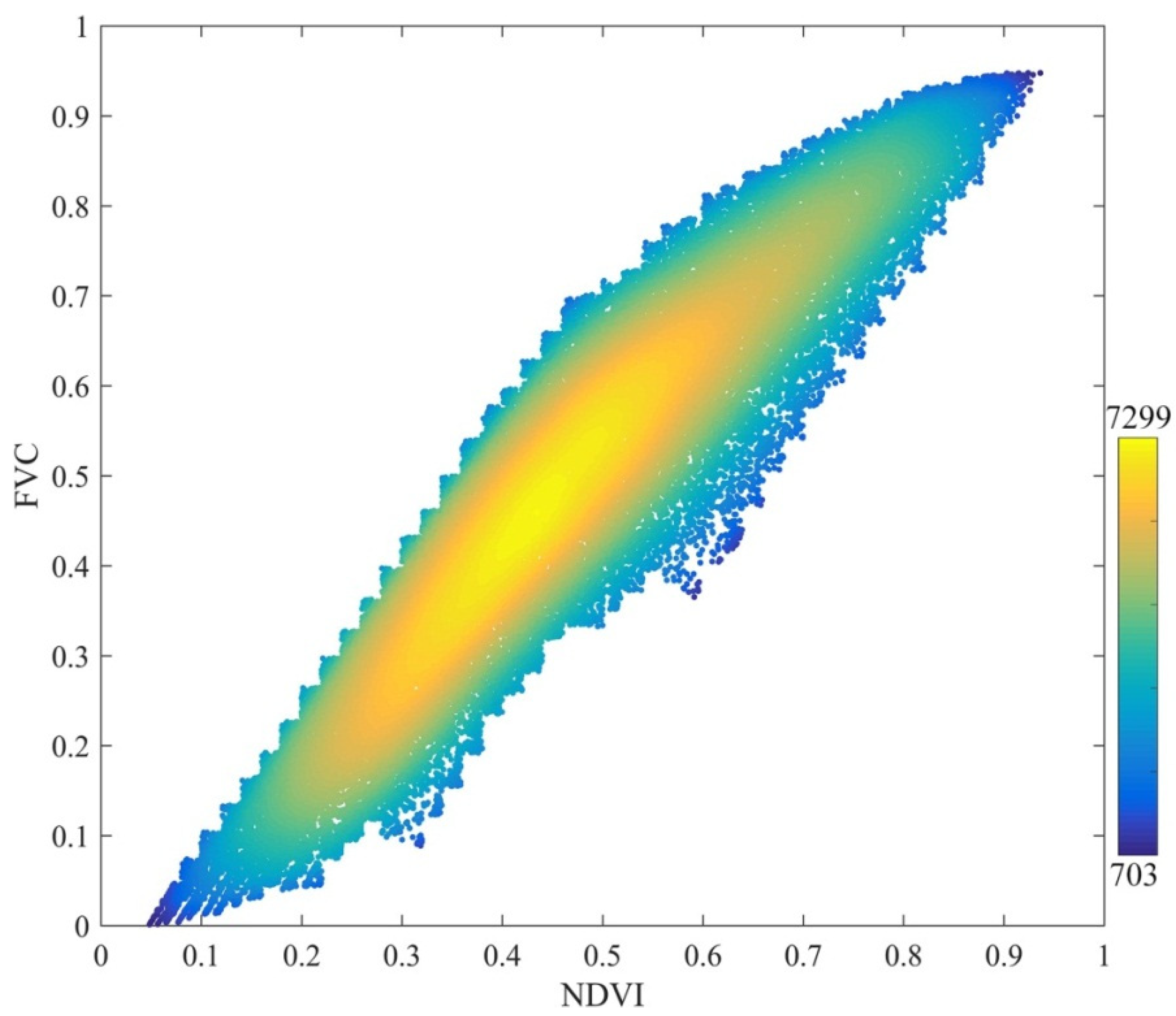
4.1. Samples of Refinement and Theoretical Validation

After the refinement of simulated samples, 40,018 high-quality samples were generated (28,012 samples for the training dataset and 12,006 samples for the validation dataset). Figure 3 presents the density scatter plot of the refined NDVI and FVC values [66]. Visibly, the approximate linear relationship between the NDVI and FVC was found, which presented the reliability of the sample data. Due to the spectral diversity of different land surface vegetation types, the spectral characterization would vary with same FVC value. Consequently, the relationship between the NDVI and FVC in Figure 3 is not strictly linear.
With these refined high-quality sample data, the random forest regression FVC estimation algorithm for FY-3B reflectance was established. In this study, 250 regression trees were determined by evaluating the accuracy performance (root mean square error; RMSE) of the FVC estimations under different quantity of regression trees based on the validation samples. Consequently, Figure 4 shows the theoretical performance of the trained random forest regression FVC estimation algorithm based on the validation samples. The FVC estimation data achieved a satisfactory performance (R2 = 0.9092, RMSE = 0.0696). Generally, the most scatter points are located around the 1:1 line, and the fitted line is close to the 1:1 line. Although there are few points located a little far from the 1:1 line, these points accounted for a tiny percentage of the whole number of the validation samples.

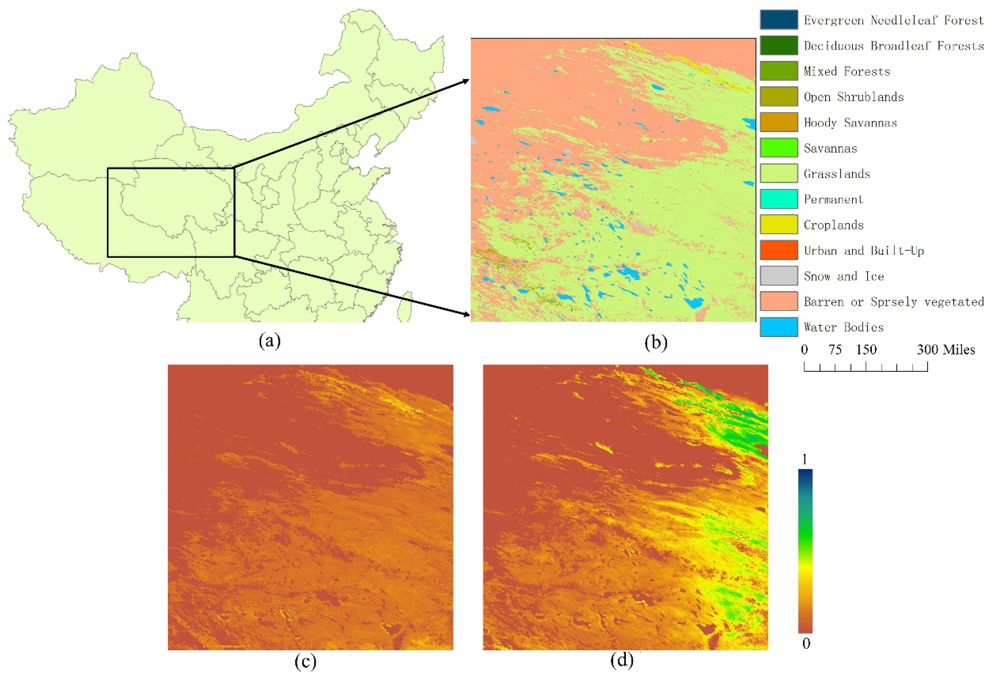
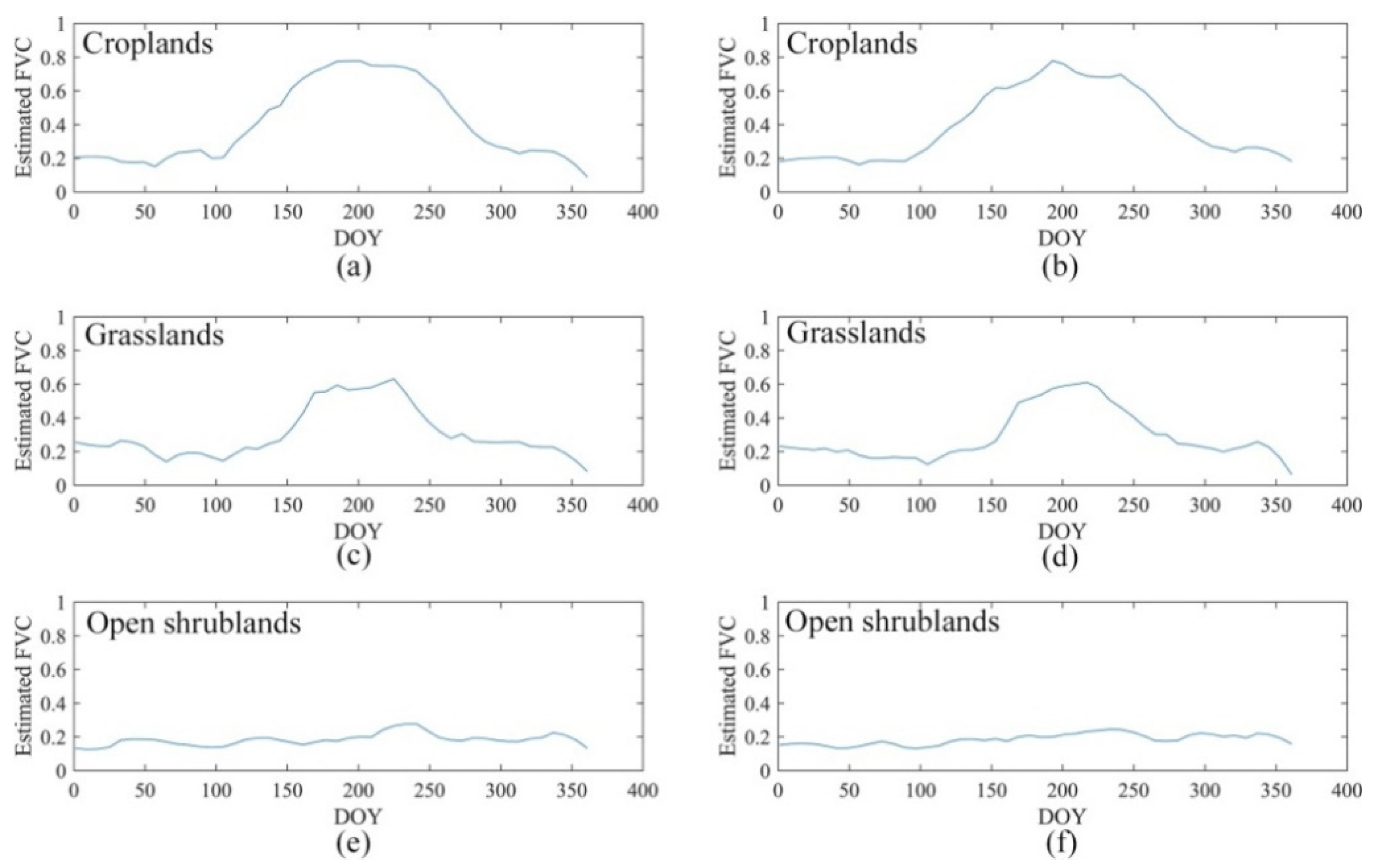
4.2. Spatial–Temporal Validation

The averaged FVC maps in January and July of 2015 over the regional areas (tile H25V05) were generated using the proposed algorithm, and Figure 5 presents the spatial distribution pattern of the FVC estimation. This area is in the mid-west region of China, which is primarily covered by montane grass, shrub, Mediterranean forest, and scrub [67]. Thus, it was reasonable to select this area to validate the spatial–temporal performance of the FVC estimation by the proposed algorithm. Visually, these monthly averaged FVC estimation maps showed stable spatial continuity, and no missing data were found. In addition, the distribution patterns of the generated FVC maps matched the actual seasonal variations and distribution of the land vegetation conditions. For example, during the summertime, high FVC values were observed in northeast region covered by grass and crops. The west and southwest regions over this area showed low FVC values, where sparse shrub and barren lands were the primary land cover types.
Figure 6 shows several representative FVC temporal profiles estimated from the FY-3B reflectance data in the Heihe River Basin over croplands, grasslands, and open shrublands. Generally, these FVC estimation profiles are temporally consistent with the seasonal phonological changes and corresponding vegetation types. Furthermore, these temporal profiles present steady variations over time, which indicate that the proposed algorithm is capable of describing the temporal characteristics of vegetation growth conditions. All these results provide strong evidence that the proposed algorithm could effectively generate FVC estimations with reliable continuities in space and time.

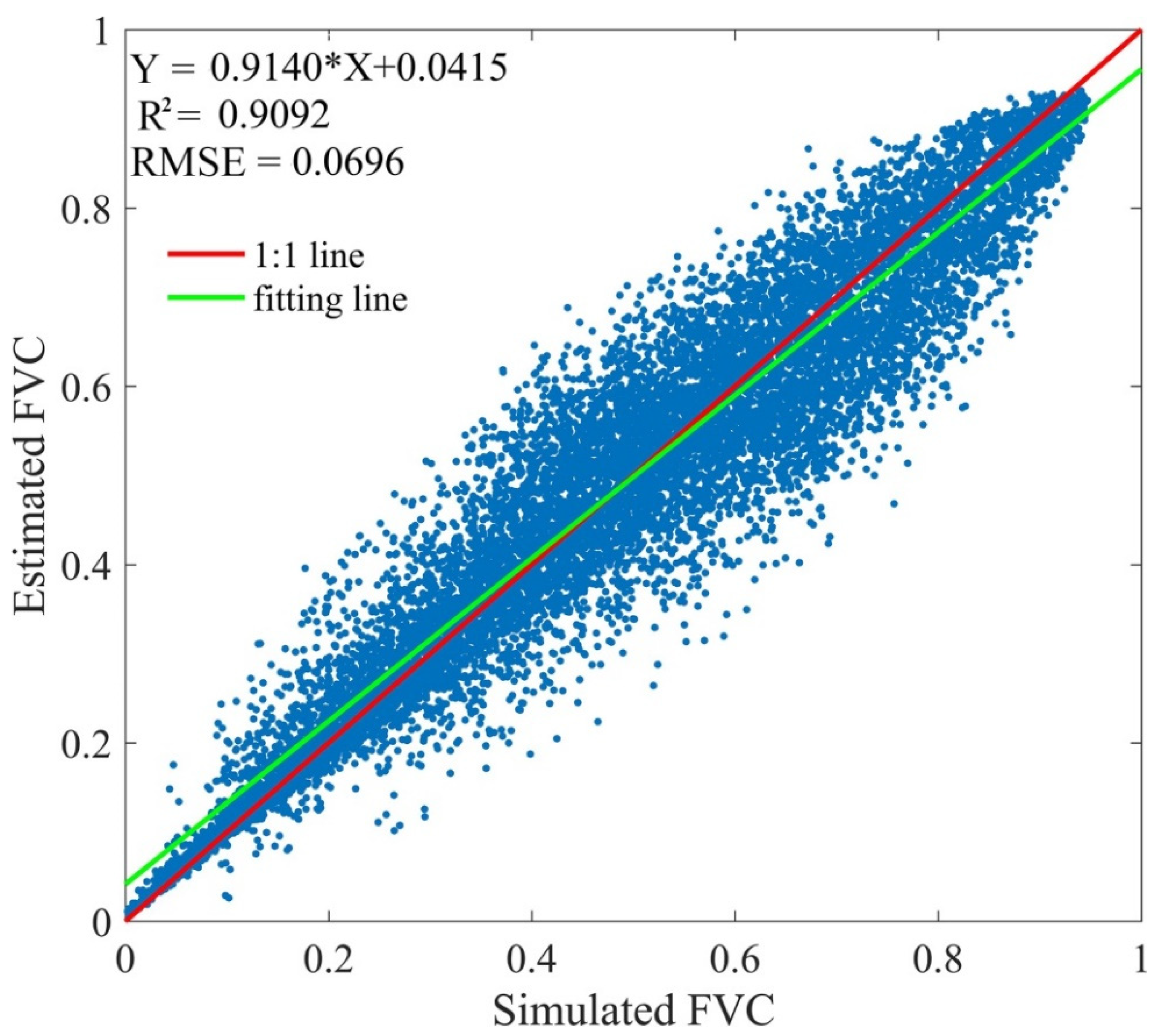
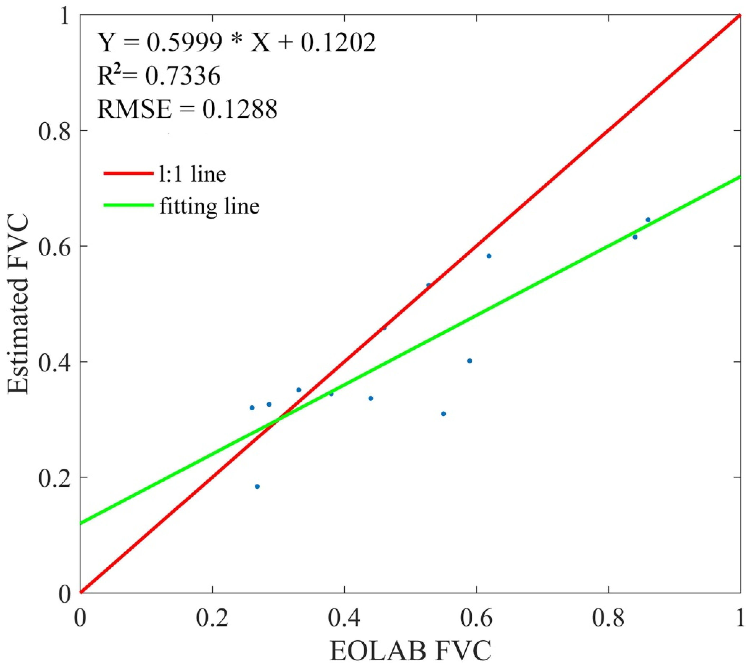
4.3. Accuracy Validation over Reference FVC Data

Since the EOLAB reference FVC data are aggregated over a 3 km × 3 km area, the averaged value of the 5 × 5 pixel subset covering each ground site was calculated for validation. Figure 7 presents the scatter plot of the FVC estimation generated by the proposed algorithm and the corresponding EOLAB reference FVC data. Overall, the FVC estimations by the proposed algorithm showed considerable consistency, with a R2 of 0.7336 and RMSE of 0.1288. Mostly, the scatter points of the reference FVC estimations and reference values lied around the 1:1 line. Besides, the EOLAB reference FVC data contained various vegetation types, which further indicated the reliability and reasonability of the proposed algorithm.

5. Discussion

During the prior studies, several FVC estimation products have been proposed based on remote sensing data and widely used in related research fields. In order to further expand earth observation sources on FVC estimating and maintain the continuity of the FVC products, this study assessed the capability of FY-3 reflectance data on FVC estimating. To reach this target, a randomly forest model was built based on the simulated FY-3B reflectance data and corresponding FVC values. With the satisfying validation results in spatial–temporal continuities and high accuracy against the reference FVC values, the FY-3B reflectance data presented a reliable performance in FVC estimation. Besides, these results confirmed that the FY-3B reflectance data were reliable land surface observation sources for FVC product generation.
Although the FVC estimations generated by the proposed algorithm presented reliable spatial–temporal continuities and accuracy based on the FY-3B reflection, several aspects need to be further explored to improve the quality of FVC estimations: (1) According to the validation samples, the theoretical validation presents higher accuracy compared with the ground validation, because there are some variabilities between the real observation and simulated data. Thus, a further quantification for the uncertainties of the simulated samples from radiative transfer model should be investigated. (2) Over the postprocessing operations, the FVC estimation data are composited by choosing the maximum FVC value during the corresponding temporal period, because the maximum FVC value would usually present the best growth state of vegetation over this time. However, the maximum value is susceptible to some atmospheric conditions. The mean value, which could reflect the general level and is robust to extreme values, of the FVC estimation is an alternative index to determine the reliable FVC estimation during this time. Besides, another approach composited the FY-3B reflectance data before estimating the FVC. Thus, investigating the performance of difference indices and approaches for the composition process is significant to further improve the quality of the FVC estimation form FY-3 data. To further confirm the ability of FY-3 reflectance data on FVC product generation, three potential operations would be conducted in our future work. Firstly, more validations and assessments for the developed algorithm would be organized under various land conditions and vegetation types, which would provide comprehensive evaluations. Besides, comparing it with some existing large-scale FVC products, like GLASS FVC and GEOV2 FVC, would be a considerable approach for the evaluation process. Secondly, some other machine learning methods, like the artificial neural network (ANN) [17], support vector regression (SVR) model [68], and multivariate adaptive regression splines (MARS) model, were adopted for FVC estimating. Thus, investigating the performances of these methods on the FVC estimation for FY-3 reflectance would be significant in the future. In addition, several empirical and pixel unmixing methods also achieved reliable FVC estimation with the regional scale [69,70,71], which would be evaluated for FY-3 FVC estimation during the future work. Finally, this study adopted the FY-3B reflectance as the representative to analyze the capability of FY-3 data on global FVC estimating. However, there are three more satellites of the FY-3 series, including FY-3A, FY-3C, and FY-3D. Therefore, combining these different FY-3 satellite data on the global FVC estimation would be a potential approach to further explore the potential of FY-3 data on large/global FVC estimation generation and improve the spatial–temporal continuities of the FVC estimations.

6. Conclusions

To investigate the capability of FY-3 reflectance data on FVC estimation, a FVC estimation algorithm for FY-3B reflectance data was developed in this study. The algorithm was established based on the PROSAIL radiative transfer model and random forest model. Both the theoretical and direct validation results indicated that the proposed algorithm could achieve satisfactory FVC estimation accuracy. Furthermore, the spatial–temporal validation over the regional area further confirmed the robustness and strong potential of the proposed algorithm on global FVC estimating with spatial and temporal continuities. The future work will focus on extensive assessment of the proposed algorithm under various land conditions.

Author Contributions

Conceptualization, D.L. and K.J.; data curation, D.L., H.J., and B.W.; methodology, D.L., H.J., and B.W.; validation, D.L., visualization, D.L.; writing—original draft, D.L.; formal analysis, K.J.; project administration, K.J.; supervision, K.J.; resources, K.J.; and writing—review and editing, K.J., M.X., G.T., Z.C., B.Y., and J.L. All authors have read and agreed to the published version of the manuscript.

Funding

This study was supported by the National Key Research and Development Program of China (2018YFA0605503), the National Natural Science Foundation of China (No. 41671332) and the Tang Scholar Program (Kun Jia is a Tang Scholar of Beijing Normal University).

Institutional Review Board Statement

Not applicable.

Informed Consent Statement

Informed consent was obtained from all subjects involved in the study.

Data Availability Statement

The FY-3B reflectance data used in this study are available in “http://www.geodoi.ac.cn/WebCn/Default.aspx”, accessed on 15 March 2021, and the EOLAB reference FVC data are obtained in “http://fp7-imagines.eu/pages/services-and-products/ground-data.php”, accessed on 15 March 2021.

Conflicts of Interest

The authors declare no conflict of interest.

References

  1. Baret, F.; Weiss, M.; Lacaze, R.; Camacho, F.; Makhmara, H.; Pacholcyzk, P.; Smets, B. GEOV1: LAI and FAPAR essential climate variables and FCOVER global time series capitalizing over existing products. Part1: Principles of development and production. Remote Sens. Environ. 2013, 137, 299–309. [Google Scholar] [CrossRef]
  2. Weiss, M.; Baret, F.; Myneni, R.B.; Pragnère, A.; Knyazikhin, Y. Investigation of a model inversion technique to estimate canopy biophysical variables from spectral and directional reflectance data. Agronomie 2000, 20, 3–22. [Google Scholar] [CrossRef]
  3. Tu, Y.; Jia, K.; Wei, X.; Yao, Y.; Xia, M.; Zhang, X.; Jiang, B. A Time-Efficient Fractional Vegetation Cover Estimation Method Using the Dynamic Vegetation Growth Information from Time Series GLASS FVC Product. IEEE Geosci. Remote Sens. Lett. 2020, 17, 1672–1676. [Google Scholar] [CrossRef]
  4. Zeng, X.; Dickinson, R.E.; Walker, A.; Shaikh, M.; DeFries, R.S.; Qi, J. Derivation and evaluation of global 1-km fractional vegetation cover data for land modeling. J. Appl. Meteorol. 2000, 39, 826–839. [Google Scholar] [CrossRef]
  5. Gutman, G.; Ignatov, A. The derivation of the green vegetation fraction from NOAA/AVHRR data for use in numerical weather prediction models. Int. J. Remote Sens. 1998, 19, 1533–1543. [Google Scholar] [CrossRef]
  6. Roujean, J.; Lacaze, R. Global mapping of vegetation parameters from POLDER multiangular measurements for studies of surface-atmosphere interactions: A pragmatic method and its validation. J. Geophys. Res. 2002, 107. [Google Scholar] [CrossRef]
  7. Jia, K.; Yang, L.; Liang, S.; Xiao, Z.; Zhao, X.; Yao, Y.; Zhang, X.; Jiang, B.; Liu, D. Long-term Global Land Surface Satellite (GLASS) fractional vegetation cover product derived from MODIS and AVHRR Data. IEEE J. Sel. Top. Appl. Earth Obs. Remote Sens. 2019, 12, 508–518. [Google Scholar] [CrossRef]
  8. Liu, D.; Jia, K.; Wei, X.; Xia, M.; Zhang, X.; Yao, Y.; Zhang, X.; Wang, B. Spatiotemporal Comparison and Validation of Three Global-Scale Fractional Vegetation Cover Products. Remote Sens. 2019, 11, 2524. [Google Scholar] [CrossRef] [Green Version]
  9. García-Haro, F.; Camacho, F.; Verger, A.; Meliá, J. Current status and potential applications of the LSA SAF suite of vegetation products. In Proceedings of the 29th EARSeL Symposium, Chania, Greece, 15–18 June 2009; pp. 15–18. [Google Scholar]
  10. Baret, F.; Hagolle, O.; Geiger, B.; Bicheron, P.; Miras, B.; Huc, M.; Berthelot, B.; Niño, F.; Weiss, M.; Samain, O. LAI, fAPAR and fCover CYCLOPES global products derived from VEGETATION: Part 1: Principles of the algorithm. Remote Sens. Environ. 2007, 110, 275–286. [Google Scholar] [CrossRef] [Green Version]
  11. Wang, X.; Jia, K.; Liang, S.; Zhang, Y. Fractional Vegetation Cover Estimation Method Through Dynamic Bayesian Network Combining Radiative Transfer Model and Crop Growth Model. IEEE Trans. Geosci. Remote Sens. 2016, 54, 7442–7450. [Google Scholar] [CrossRef]
  12. Mu, X.; Huang, S.; Ren, H.; Yan, G.; Song, W.; Ruan, G. Validating GEOV1 fractional vegetation cover derived from coarse-resolution remote sensing images over croplands. IEEE J. Sel. Top. Appl. Earth Obs. Remote Sens. 2014, 8, 439–446. [Google Scholar] [CrossRef]
  13. Baret, F.; Pavageau, K.; Béal, D.; Weiss, M.; Berthelot, B.; Regner, P. Algorithm Theoretical Basis Document for MERIS Top of Atmosphere Land Products (TOA_VEG); INRA-CSE: Avignon, France, 2006. [Google Scholar]
  14. Verger, A.; Baret, F.; Weiss, M. GEOV2/VGT: Near real time estimation of global biophysical variables from VEGETATION-P data. In Proceedings of the MultiTemp 7th International Workshop on the Analysis of Multi-temporal Remote Sensing Images, Banff, AB, Canada, 25–27 June 2013; pp. 1–4. [Google Scholar]
  15. Baret, F.; Weiss, M.; Verger, A.; Smets, B. ATBD for LAI, FAPAR and FCOVER From PROBA-V Products at 300M Resolution (GEOV3). IMAGINES_RP2. 1_ATBD-LAI300M. 2016. Available online: http://www.fp7-imagines.eu/media/Documents/ImagineS_RP2.1_ATBD-LAI300m_I1.73.pdf (accessed on 14 May 2021).
  16. Jia, K.; Liang, S.; Liu, S.; Li, Y.; Xiao, Z.; Yao, Y.; Jiang, B.; Zhao, X.; Wang, X.; Xu, S. Global land surface fractional vegetation cover estimation using general regression neural networks from MODIS surface reflectance. IEEE Trans. Geosci. Remote Sens. 2015, 53, 4787–4796. [Google Scholar] [CrossRef]
  17. Yang, L.; Jia, K.; Liang, S.; Liu, J.; Wang, X. Comparison of four machine learning methods for generating the GLASS fractional vegetation cover product from MODIS data. Remote Sens. 2016, 8, 682. [Google Scholar] [CrossRef] [Green Version]
  18. Xiong, X.; Sun, J.; Barnes, W.; Salomonson, V.; Esposito, J.; Erives, H.; Guenther, B. Multiyear on-orbit calibration and performance of Terra MODIS reflective solar bands. IEEE Trans. Geosci. Remote Sens. 2007, 45, 879–889. [Google Scholar] [CrossRef]
  19. Zhang, W. Status and development of FY series of meteorological satellites. Aerosp. Shanghai 2001, 2, 8–13. [Google Scholar]
  20. Yang, J. Development and applications of China’s Fengyun (FY) meteorological satellite. Spacecr. Eng. 2008, 17, 23–28. [Google Scholar]
  21. Dong, C.; Yang, J.; Zhang, W.; Yang, Z.; Lu, N.; Shi, J.; Zhang, P.; Liu, Y.; Cai, B. An overview of a new Chinese weather satellite FY-3A. Bull. Am. Meteorol. Soc. 2009, 90, 1531–1544. [Google Scholar] [CrossRef]
  22. Zhong, Y.; Wang, X.; Wang, S.; Zhang, L. Advances in spaceborne hyperspectral remote sensing in China. Geo. Spat. Inf. Sci. 2021, 24, 1–26. [Google Scholar] [CrossRef]
  23. Yang, J.; Zhang, P.; Lu, N.; Yang, Z.; Shi, J.; Dong, C. Improvements on global meteorological observations from the current Fengyun 3 satellites and beyond. Int. J. Digit. Earth 2012, 5, 251–265. [Google Scholar] [CrossRef]
  24. Yang, J.; Dong, C.-h.; Lu, N.-m.; Yang, Z.; Shi, J.; Zhang, P.; Liu, Y.; Cai, B. FY-3A: The new generation polar-orbiting meteorological satellite of China. Acta Meteorol. Sin. 2009, 67, 501–509. [Google Scholar]
  25. García-Haro, F.J.; Camacho-de Coca, F.; Miralles, J.M. Inter-comparison of SEVIRI/MSG and MERIS/ENVISAT biophysical products over Europe and Africa. In Proceedings of Proceedings of the 2nd MERIS/(A) ATSR User Workshop, Frascati, Italy, 22–26 September 200; pp. 22–26.
  26. Wang, Z.; Deng, R.; Ma, P.; Zhang, Y.; Liang, Y.; Chen, H.; Zhao, S.; Chen, L. 250-m Aerosol Retrieval from FY-3 Satellite in Guangzhou. Remote Sens. 2021, 13, 920. [Google Scholar] [CrossRef]
  27. Yang, Z.; Lu, N.; Shi, J.; Zhang, P.; Dong, C.; Yang, J. Overview of FY-3 Payload and Ground Application System. IEEE Trans. Geosci. Remote Sens. 2012, 50, 4846–4853. [Google Scholar] [CrossRef]
  28. Jiapaer, G.; Chen, X.; Bao, A. A comparison of methods for estimating fractional vegetation cover in arid regions. Agric. For. Meteorol. 2011, 151, 1698–1710. [Google Scholar] [CrossRef]
  29. Carlson, T.N.; Ripley, D.A. On the relation between NDVI, fractional vegetation cover, and leaf area index. Remote Sens. Environ. 1997, 62, 241–252. [Google Scholar] [CrossRef]
  30. Lyu, D.; Liu, B.; Zhang, X.; Yang, X.; He, L.; He, J.; Guo, J.; Wang, J.; Cao, Q. An Experimental Study on Field Spectral Measurements to Determine Appropriate Daily Time for Distinguishing Fractional Vegetation Cover. Remote Sens. 2020, 12, 2942. [Google Scholar] [CrossRef]
  31. Liu, D.; Yang, L.; Jia, K.; Liang, S.; Xiao, Z.; Wei, X.; Yao, Y.; Xia, M.; Li, Y. Global fractional vegetation cover estimation algorithm for VIIRS reflectance data based on machine learning methods. Remote Sens. 2018, 10, 1648. [Google Scholar] [CrossRef] [Green Version]
  32. Sun, L.; Hu, X.; Xu, N.; Liu, J.; Zhang, L.; Rong, Z. Postlaunch calibration of FengYun-3B MERSI reflective solar bands. IEEE Trans. Geosci. Remote Sens. 2012, 51, 1383–1392. [Google Scholar]
  33. Sun, L.; Hu, X.; Chen, L. Long-term calibration monitoring of medium resolution spectral imager (MERSI) solar bands onboard FY-3. In Proceedings of the Earth Observing Missions and Sensors: Development, Implementation, and Characterization II, Kyoto, Japan, 29 October–1 November 2012; p. 852808. [Google Scholar]
  34. Zhang, X.; Zhu, L.; Sun, H.; Chu, S. Validation and inter-comparison of the FY-3B/MERSI LAI product with GLOBMAP and MYD15A2H. Int. J. Remote Sens. 2020, 41, 9256–9282. [Google Scholar] [CrossRef]
  35. Li, W.; Baret, F.; Weiss, M.; Buis, S.; Lacaze, R.; Demarez, V.; Dejoux, J.-f.; Battude, M.; Camacho, F. Combining hectometric and decametric satellite observations to provide near real time decametric FAPAR product. Remote Sens. Environ. 2017, 200, 250–262. [Google Scholar] [CrossRef]
  36. Mu, X.; Zhao, T.; Ruan, G.; Song, J.; Wang, J.; Yan, G.; Mcvicar, T.R.; Yan, K.; Gao, Z.; Liu, Y. High Spatial Resolution and High Temporal Frequency (30-m/15-day) Fractional Vegetation Cover Estimation over China Using Multiple Remote Sensing Datasets: Method Development and Validation. J. Meteorol. Res. 2021, 35, 128–147. [Google Scholar] [CrossRef]
  37. Morisette, J.T.; Baret, F.; Privette, J.L.; Myneni, R.B.; Nickeson, J.E.; Garrigues, S.; Shabanov, N.V.; Weiss, M.; Fernandes, R.A.; Leblanc, S.G. Validation of global moderate-resolution LAI products: A framework proposed within the CEOS land product validation subgroup. IEEE Trans. Geosci. Remote Sens. 2006, 44, 1804–1817. [Google Scholar] [CrossRef] [Green Version]
  38. Camacho, F.; Lacaze, R.; Latorre, C.; Baret, F.; De la Cruz, F.; Demarez, V.; Di Bella, C.; García-Haro, J.; González-Dugo, M.P.; Kussul, N.; et al. Collection of Ground Biophysical Measurements in support of Copernicus Global Land Product Validation: The ImagineS database. In Proceedings of the EGU General Assembly Conference Abstracts, Vienna, Austria, 12–17 April 2015; p. 2209. [Google Scholar]
  39. Jacquemoud, S.; Verhoef, W.; Baret, F.; Bacour, C.; Zarco-Tejada, P.J.; Asner, G.P.; François, C.; Ustin, S.L. PROSPECT+ SAIL models: A review of use for vegetation characterization. Remote Sens. Environ. 2009, 113, S56–S66. [Google Scholar] [CrossRef]
  40. Allen, W.A.; Gausman, H.W.; Richardson, A.J.; Thomas, J.R. Interaction of isotropic light with a compact plant leaf. Josa 1969, 59, 1376–1379. [Google Scholar] [CrossRef]
  41. Yang, L.; Deng, S.; Zhang, Z. New spectral model for estimating leaf area index based on gene expression programming. Comput. Electr. Eng. 2020, 83, 106604. [Google Scholar] [CrossRef]
  42. Verhoef, W. Light scattering by leaf layers with application to canopy reflectance modeling: The SAIL model. Remote Sens. Environ. 1984, 16, 125–141. [Google Scholar] [CrossRef] [Green Version]
  43. Nilson, T. A theoretical analysis of the frequency of gaps in plant stands. Agric. Meteorol. 1971, 8, 25–38. [Google Scholar] [CrossRef]
  44. Yang, L.; Jia, K.; Liang, S.; Wei, X.; Yao, Y.; Zhang, X. A robust algorithm for estimating surface fractional vegetation cover from landsat data. Remote Sens. 2017, 9, 857. [Google Scholar] [CrossRef] [Green Version]
  45. Shepherd, K.D.; Palm, C.A.; Gachengo, C.N.; Vanlauwe, B. Rapid characterization of organic resource quality for soil and livestock management in tropical agroecosystems using near-infrared spectroscopy. Agron. J. 2003, 95, 1314–1322. [Google Scholar] [CrossRef] [Green Version]
  46. He, B.; Liao, Z.; Quan, X.; Li, X.; Hu, J. A global Grassland Drought Index (GDI) product: Algorithm and validation. Remote Sens. 2015, 7, 12704–12736. [Google Scholar] [CrossRef] [Green Version]
  47. Dennison, P.E.; Halligan, K.Q.; Roberts, D.A. A comparison of error metrics and constraints for multiple endmember spectral mixture analysis and spectral angle mapper. Remote Sens. Environ. 2004, 93, 359–367. [Google Scholar] [CrossRef]
  48. Jia, K.; Li, Q.-Z.; Tian, Y.-C.; Wu, B.-F.; Zhang, F.-F.; Meng, J.-H. Accuracy improvement of spectral classification of crop using microwave backscatter data. Spectrosc. Spectr. Anal. 2011, 31, 483–487. [Google Scholar]
  49. Jia, K.; Liang, S.; Gu, X.; Baret, F.; Wei, X.; Wang, X.; Yao, Y.; Yang, L.; Li, Y. Fractional vegetation cover estimation algorithm for Chinese GF-1 wide field view data. Remote Sens. Environ. 2016, 177, 184–191. [Google Scholar] [CrossRef]
  50. Tu, Y.; Jia, K.; Liang, S.; Wei, X.; Yao, Y.; Zhang, X. Fractional vegetation cover estimation in heterogeneous areas by combining a radiative transfer model and a dynamic vegetation model. Int. J. Digit. Earth 2020, 13, 487–503. [Google Scholar] [CrossRef]
  51. Fernández-Guisuraga, J.M.; Verrelst, J.; Calvo, L.; Suárez-Seoane, S. Hybrid inversion of radiative transfer models based on high spatial resolution satellite reflectance data improves fractional vegetation cover retrieval in heterogeneous ecological systems after fire. Remote Sens. Environ. 2021, 255, 112304. [Google Scholar] [CrossRef]
  52. Mutanga, O.; Adam, E.; Cho, M.A. High density biomass estimation for wetland vegetation using WorldView-2 imagery and random forest regression algorithm. Int. J. Appl. Earth Obs. Geoinf. 2012, 18, 399–406. [Google Scholar] [CrossRef]
  53. Izquierdo-Verdiguier, E.; Zurita-Milla, R. An evaluation of Guided Regularized Random Forest for classification and regression tasks in remote sensing. Int. J. Appl. Earth Obs. Geoinf. 2020, 88, 102051. [Google Scholar] [CrossRef]
  54. Zhang, X.; He, G.; Zhang, Z.; Peng, Y.; Long, T. Spectral-spatial multi-feature classification of remote sensing big data based on a random forest classifier for land cover mapping. Clust. Comput. 2017, 20, 2311–2321. [Google Scholar] [CrossRef]
  55. Jin, X.-l.; Diao, W.-y.; Xiao, C.-h.; Wang, F.-y.; Chen, B.; Wang, K.-r.; Li, S.-k. Estimation of wheat agronomic parameters using new spectral indices. PLoS ONE 2013, 8, e72736. [Google Scholar] [CrossRef] [PubMed] [Green Version]
  56. Zhou, X.; Zhu, X.; Dong, Z.; Guo, W. Estimation of biomass in wheat using random forest regression algorithm and remote sensing data. Crop J. 2016, 4, 212–219. [Google Scholar]
  57. Wang, B.; Jia, K.; Liang, S.; Xie, X.; Wei, X.; Zhao, X.; Yao, Y.; Zhang, X. Assessment of Sentinel-2 MSI spectral band reflectances for estimating fractional vegetation cover. Remote Sens. 2018, 10, 1927. [Google Scholar] [CrossRef] [Green Version]
  58. Ben Ishak, A. Variable selection using support vector regression and random forests: A comparative study. Intell. Data Anal. 2016, 20, 83–104. [Google Scholar] [CrossRef]
  59. Yang, Y.; Cao, C.; Pan, X.; Li, X.; Zhu, X. Downscaling land surface temperature in an arid area by using multiple remote sensing indices with random forest regression. Remote Sens. 2017, 9, 789. [Google Scholar] [CrossRef] [Green Version]
  60. Nieto, P.G.; Garcia-Gonzalo, E.; Paredes-Sánchez, J.P.; Sánchez, A.B.; Fernández, M.M. Predictive modelling of the higher heating value in biomass torrefaction for the energy treatment process using machine-learning techniques. Neural Comput. Appl. 2019, 31, 8823–8836. [Google Scholar] [CrossRef]
  61. Yuan, Q.; Li, S.; Yue, L.; Li, T.; Shen, H.; Zhang, L. Monitoring the Variation of Vegetation Water Content with Machine Learning Methods: Point–Surface Fusion of MODIS Products and GNSS-IR Observations. Remote Sens. 2019, 11, 1440. [Google Scholar] [CrossRef] [Green Version]
  62. Wang, B.; Jia, K.; Wei, X.; Xia, M.; Yao, Y.; Zhang, X.; Liu, D.; Tao, G. Generating spatiotemporally consistent fractional vegetation cover at different scales using spatiotemporal fusion and multiresolution tree methods. ISPRS J. Photogramm. Remote Sens. 2020, 167, 214–229. [Google Scholar] [CrossRef]
  63. Savitzky, A.; Golay, M.J. Smoothing and differentiation of data by simplified least squares procedures. Anal. Chem. 1964, 36, 1627–1639. [Google Scholar] [CrossRef]
  64. Kim, S.-R.; Prasad, A.K.; El-Askary, H.; Lee, W.-K.; Kwak, D.-A.; Lee, S.-H.; Kafatos, M. Application of the Savitzky-Golay filter to land cover classification using temporal MODIS vegetation indices. Photogramm. Eng. Remote Sens. 2014, 80, 675–685. [Google Scholar] [CrossRef]
  65. Fang, H.; Liang, S.; Hoogenboom, G. Integration of MODIS LAI and vegetation index products with the CSM–CERES–Maize model for corn yield estimation. Int. J. Remote Sens. 2011, 32, 1039–1065. [Google Scholar] [CrossRef]
  66. Sanchez, A. Scatplot. Available online: https://www.mathworks.com/matlabcentral/fileexchange/8577-scatplot (accessed on 14 May 2021).
  67. Olson, D.M.; Dinerstein, E.; Wikramanayake, E.D.; Burgess, N.D.; Powell, G.V.N.; Underwood, E.C.; D’Amico, J.A.; Itoua, I.; Strand, H.E.; Morrison, J.C.; et al. Terrestrial Ecoregions of the World: A New Map of Life on Earth: A new global map of terrestrial ecoregions provides an innovative tool for conserving biodiversity. BioScience 2001, 51, 933–938. [Google Scholar] [CrossRef]
  68. Tuia, D.; Verrelst, J.; Alonso, L.; Pérez-Cruz, F.; Camps-Valls, G. Multioutput support vector regression for remote sensing biophysical parameter estimation. IEEE Geosci. Remote Sens. Lett. 2011, 8, 804–808. [Google Scholar] [CrossRef]
  69. Gitelson, A.A.; Kaufman, Y.J.; Stark, R.; Rundquist, D. Novel algorithms for remote estimation of vegetation fraction. Remote Sens. Environ. 2002, 80, 76–87. [Google Scholar] [CrossRef] [Green Version]
  70. Jiménez-Gutiérrez, J.M.; Valero, F.; Jerez, S.; Montávez, J.P. Impacts of green vegetation fraction derivation methods on regional climate simulations. Atmosphere 2019, 10, 281. [Google Scholar] [CrossRef] [Green Version]
  71. Jiménez-Muñoz, J.; Sobrino, J.; Guanter, L.; Moreno, J.; Plaza, A.; Martínez, P. Fractional vegetation cover estimation from PROBA/CHRIS data: Methods, analysis of angular effects and application to the land surface emissivity retrieval. In Proceedings of the 3rd Workshop CHRIS/Proba Workshop, Frascati, Italy, 21–23 March 2005. [Google Scholar]
Figure 1. FVC estimation algorithm flowchart for the FY-3B reflectance data.
Remotesensing 13 02165 g001
Figure 2. Twenty representative soil reflectance profiles after re-sample and integration.
Remotesensing 13 02165 g002
Figure 3. The distribution of the density scatter plots of the refined NDVI and FVC samples (the density value of each NDVI–FVC sample point was calculated by counting the number of splattering over a center circular area with a 0.1 length of the radius [66]).
Remotesensing 13 02165 g003
Figure 4. Theoretical performance of the random forest regression using simulated FVC data.
Remotesensing 13 02165 g004
Figure 5. Information of the study area and monthly averaged FVC estimation maps by the proposed algorithm in 2015: (a) location of the study area over China, (b) land cover data of MCD12Q1 (IGBP) for the study area, and (c,d) FVC estimations generated by the proposed algorithm in January and July, respectively.
Remotesensing 13 02165 g005
Figure 6. Temporal profiles of the FVC estimations by the proposed algorithm over different vegetation types in 2015 (a,b: croplands, c,d: grasslands, e,f: open shrublands).
Remotesensing 13 02165 g006
Figure 7. Scatter plot of the estimated FVC estimation by the proposed algorithm and the EOLAB reference FVC data.
Remotesensing 13 02165 g007
Table 1. Information on the existing FVC products over a large/global scale [7,8].
ProductsSensorMethodSpatial ResolutionTemporal ResolutionSpatial CoverageTemporal Coverage
CNES/POLDERPOLDEREmpirical model6 km10 daysGlobal1996–1997, 2003
LSA SAFSEVIRIThe pixel unmixing model3 kmDailyEurope, Africa, South American2005–present
CYCLOPESSPOT VGTMachine learning method1/112°10 daysGlobal1998–2007
ESA/MERISMERISMachine learning method300 mMonth/10 daysGlobal2002–2012
GEOV1 FVCSPOT-VEGETATIONMachine learning method1/112°10 daysGlobal1999–present
GEOV2 FVCSPOT-VEGETATION, PROBA-VMachine learning method1/112°10 daysGlobal1999–present
GEOV3 FVCPROBA-VMachine learning method300 m10 daysGlobal2014–present
GLASS FVCMODISMachine learning method500m8 daysGlobal2000-present
Table 2. Information on the FY-3B/MERSI spectral bands and specifications.
Band NumberCentral Wavelengths (μm)Band Widths (μm)Instantaneous Field of View (IFOV/m)
10.4700.05250
20.5500.05250
30.6500.05250
40.8650.05250
511.2502.50250
61.6400.051000
72.1300.051000
80.4120.021000
90.4430.021000
100.4900.021000
110.5200.021000
120.5650.021000
130.6500.021000
140.6850.021000
150.7650.021000
160.8650.021000
170.9050.021000
180.9400.021000
190.9800.021000
201.0300.021000
Table 3. Information on the EOLAB reference FVC data.
NumberNameLatitude (°)Longitude (°)YearDay of YearFVC
1SanFernando−34.7228−71.00192015190.44
2Barrax-LasTiesas39.05437−2.1006820151450.268
3Pshenichne50.0765730.2322420151740.46
4Pshenichne50.0765730.2322420151880.619
5Pshenichne50.0765730.2322420152040.528
6AHSPECT-Meteopol43.57281.374520151730.26
7AHSPECT-Peyrousse43.66620.219520151740.38
8AHSPECT-Urgons43.6397−0.434020151740.55
9AHSPECT-Creón d’Armagnac43.9936−0.046920151750.59
10AHSPECT-Condom43.97430.336020151760.331
11AHSPECT-Savenès43.82421.174920151760.286
12Collelongo41.8513.5920151890.84
13Collelongo41.8513.5920152660.86
Table 4. Input parameters for the PROSAIL model.
ModelParametersRange or Fixed Value
( V a , σ )
PROSPECTLeaf structure parameter (N)1~2.5(1.5, 1)
Chlorophyll content (Cab, μg/cm 2)30~100(50, 30)
Brown pigment (Cbrown)0~1.5(0.1, 0.2)
Dry matter content (Cm, g/cm 2)0.002~0.02(0.0075, 0.0075)
Relative water content0.65~0.90(0.8, 0.05)
SAILFractional vegetation coverage (FVC)0~0.95(0.5, 0.4)
Average leaf angle (ALA,°)30~70(50, 15)
Hot spot parameter (hspot)0.001~1(0.1, 0.3)
Sun zenith angle (SAZ, ◦)30-
Observer zenith angle (OZA, ◦)0-
Relative azimuth angle(RAA, ◦)0-
Soil reflectanceid:1~20--
Publisher’s Note: MDPI stays neutral with regard to jurisdictional claims in published maps and institutional affiliations.

