
Lane Crack Detection Based on Saliency


1
School of Remote Sensing and Information Engineering, Wuhan University, Wuhan 430079, China
2
Henan Provincial Transportation Development Center, Zhengzhou 450016, China
*
Author to whom correspondence should be addressed.
Remote Sens. 2023, 15(17), 4146; https://doi.org/10.3390/rs15174146
Submission received: 2 July 2023
/
Revised: 15 August 2023
/
Accepted: 15 August 2023
/
Published: 24 August 2023
Abstract
:Lane cracks are one of the biggest threats to pavement conditions. The automatic detection of lane cracks can not only assist the evaluation of road quality and quantity but can also be used to develop the best crack repair plan, so as to keep the road level and ensure driving safety. Although cracks can be extracted from pavement images because the gray intensity of crack pixels is lower than the background gray intensity, it is still a challenge to extract continuous and complete cracks from the three-lane images with complex texture, high noise, and uneven illumination. Different from threshold segmentation and edge detection, this study designed a crack detection algorithm with dual positioning. An image-enhancement method based on crack saliency is proposed for the first time. Based on Bayesian probability, the saliency of each pixel judged as a crack is calculated. Then, the Fréchet distance improvement triangle relationship is introduced to determine whether the key point extracted is the fracture endpoint and whether the fast-moving method should be terminated. In addition, a complete remote-sensing process was developed to calculate the length and width of cracks by inverting the squint images collected by mobile phones. A large number of images with different types, noise, illumination, and interference conditions were tested. The average crack extraction accuracy of 89.3%, recall rate of 87.1%, and F1 value of 88.2% showed that the method could detect cracks in pavement well.
1. Introduction
Road cracks can occur on the pavement due to vehicle overloading, weathering, sun exposure, and waterlogged roads. Road cracks are one of the most common diseases on pavement, which can endanger the health and sustainable use of highways. Cracks are a sign of road damage. Cracks have “accelerated growth” properties. When cracks appear on the pavement without timely treatment, cracks will become longer and wider with the advance of time. They also cause increased maintenance cost and difficulty [1]. Accurate crack detection is the key to determine the crack grade of channel and repair the subsequent work. The traditional crack detection method is manual survey, which is not safe; it is also time-consuming and laborious. At present, it is a common engineering practice to install cameras on vehicles for image acquisition. Extracting road cracks from the collected images and calculating the size of the cracks can help the road department solve road damage conditions, so as to formulate relevant repair strategies [2].
In recent years, in order to solve the problem of pavement crack detection, people have conducted a lot of research on pavement crack detection methods. Currently, the mainstream methods based on image processing can be divided into the following three categories: (1) The first is the method based on threshold segmentation. In Reference [3], an unsupervised crack detection method based on a gray histogram and the Ostu threshold method is proposed, and good results were obtained at a low signal-to-noise ratio. In Reference [4], the crack extraction under the condition of a high signal-to-noise ratio was realized by changing the probability weighted factor of the gray histogram in the Ostu threshold method. (2) The second is the method based on edge detection. References [5,6] studied the sharp changes in the intensity of crack edges, detected the double edges of cracks to generate image gray crack profiles, and further separated the crack regions. In Reference [7], a crack detection system was designed by using morphological filtering and Canny edge detection. Reference [8] combined the Otsu threshold method with the Canny edge detection algorithm, and multi-resolution crack segmentation was realized through an adaptive analysis of global and local edge features. (3) The third is an algorithm based on salience. Such methods emphasize the difference between the crack and the background in the apparent senses, highlight the crack area, and inhibit the non-crack area, so as to achieve the purpose of separating the crack and the background. Reference [9] demonstrated the effectiveness of detecting significant regions in the Berkeley database. However, the method based on image processing cannot obtain continuous cracks, nor can it eliminate the influence of background noise.
In addition, in the field of crack detection, there is also a shortest-path method, which holds that the gray intensity of cracks is small, and the shortest path curve between the two ends of cracks is taken as input. This method was first proposed by Kass et al. [10]. In recent years, the research on crack detection based on the shortest-path algorithm has also made rich achievements. In the literature [11], the FMM algorithm introduced key points and was used for the first time to judge whether the algorithm should be stopped according to the triangular relationship. References [12,13] improved the above algorithm by selecting the endpoints on a small scale and the minimum path on a global scale, while detecting the width of cracks. Free-form anisotropy was introduced in Reference [14], and more accurate cracks were extracted by considering the pixel intensity and morphological characteristics. In Reference [15], an MPS algorithm was combined with the global gray threshold to produce clearer endpoint selection and greatly reduce the calculation time of the shortest path. Reference [16] selected candidate points by dividing cells to optimize the path search strategy and improve the efficiency and accuracy of the algorithm. In the work, cracks were extracted from 2D optical images and 3D depth images via automatic voting combined with seed sampling and attractive field. Reference [17] emphasized an effective quantification of hidden damage in composite structures by using ultrasonic guided wave (GW)-propagation-based structural health monitoring (SHM) and an artificial neural network (ANN)-based active infrared thermography (IRT) analysis. Although the crack detection algorithm based on the shortest path can extract continuous cracks, it is very dependent on the significant difference between cracks and background and requires a starting point to start the algorithm.
With the continuous increase of image data, the method based on deep learning has become an important branch of road crack detection [18]. According to the processing results, the model can be divided into two categories: (1) The first is the rough positioning model, which is mainly based on the YOLO [19] network; you can select cracks in the image box and judge their categories. Reference [20] designed a crack-tracking system based on PCGAN and the YOLO-MF network, which achieved 98.43% accuracy. Reference [21] improved the CSP layer in the backbone of YOLOv5 and introduced the pyramid divided-attention mechanism into the model for the first time. Reference [22] described a YOLOv3 model with a four-scale detection layer (FDL) that was used to detect B-scan and C-scan GPR images, and F1 Score and mAP on GPR datasets were increased by 8.7% and 5.3%, respectively. (2) The second is the accurate positioning model. Such models can pinpoint the location of cracks in the image. Through the adaptive modification of the artificial neural network, random forest, SVM, convolutional neural network and other models [23,24,25,26,27,28,29,30,31], scholars have provided a relatively good solution for crack detection. However, the rough positioning model is not accurate, and the processing time of accurate positioning is long [31].
The continuous improvement and application expansion of YOLO series algorithms also provide a reference for road crack detection. For example, in Reference [32], the improved YOLOv5-Banana model was used to identify banana fruit clusters. Reference [33] adopted YOLOv7 to improve the detection accuracy of Camellia oleifera fruits under the conditions of front lighting, backlighting, and partial occlusion. Reference [34] combined the U-net neural network algorithm and an improved image thinning algorithm to propose a method for dam crack identification and width calculation, which does not rely on a large number of training samples and avoids setting too many artificial thresholds, and it has significant practicability and stability. Reference [35] proposed a new crack backbone refinement algorithm and width measurement scheme for reservoir dams which simplified the redundant data in crack images and improved the efficiency of crack-shape estimation. Reference [36] proposed an LWMG-YOLOv5 model with ghost convolution, which improved the chip profile detection speed by 3.62% and chip yield by 1.7% and significantly reduced the production cost loss by 1.83%.
It can be found from these studies that the current crack detection methods have their own advantages and disadvantages. If the advantages of the above methods can be integrated, a fast, efficient, accurate, and robust crack extraction method can be realized. In this study, the image-processing method, the shortest-path method, and the machine-learning method were combined to make full use of the statistical significance of cracks and realize the object-based robust crack detection. First, the lightweight model of improved YOLOv5 was extended, and a large number of crack images were used for training. The improved YOLOv5 detection network was obtained, which could realize the positioning and selection of ROI in the crack region. Then, combined with the camera imaging model and the internal and external parameters of the camera, the ROI of the crack region was transformed into the reverse perspective, and the corresponding relationship between the pixel distance and the actual distance was established. The significance of each pixel at the crack point was then calculated using Bayesian probability formula and linearly stretched to increase the contrast between the crack and the background. Finally, the triangle relationship improved by Fréchet distance was used to judge whether the crack extraction was complete, and the difficult problem of spatial similarity measurement in the fast-moving method was solved. The method that was designed in this study can complete data acquisition by using very simple equipment, without the need of expensive infrared laser equipment, and the data postprocessing process is simple; the method has strong applicability and is a low-cost remote-sensing method. In this study, multiple methods were combined based on the principle of complementarity to achieve accurate crack detection under complex lighting, interference, and texture conditions. The structure diagram of the whole remote sensing process is shown in Figure 1.
The main contributions of this paper are summarized as follows:
- (a)
- A method for improved YOLOv5 and image enhancement based on crack saliency was proposed. Based on Bayesian probability, it calculates the significance of each pixel judged as a crack.
- (b)
- Fréchet distance was introduced to improve the triangle relationship to determine whether the extracted key points are the fracture endpoint and whether the fast-moving method should be terminated.
- (c)
- We developed a complete remote-sensing process that calculates the length and width of cracks by inverting oblique images collected by mobile phones.
2. Methods
2.1. Saliency Enhancement
2.1.1. Saliency Image
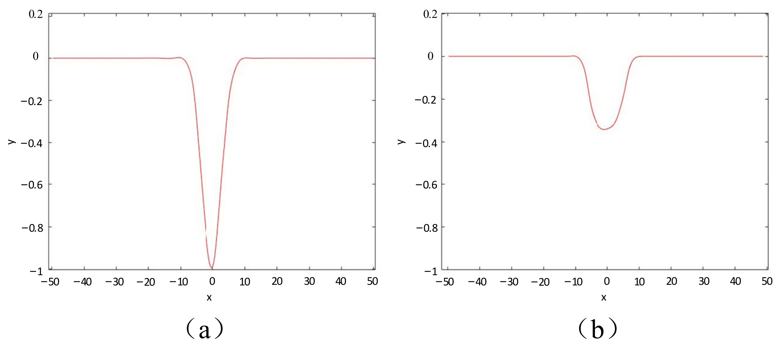
Cracks are structures with certain grayscale contrast compared to the surrounding background. The grayscale values in the crack area are lower than those in the non-crack background area. If the grayscale values of pixels are regarded as the height of the point. The cross-section along the direction perpendicular to the crack in Figure 2a is a continuous curved valley structure, and the “valley” indicated by the red line in the figure is the location of the crack. The detection of the grayscale “valley” can be used to search for cracks. However, in some cases, due to the imaging conditions, the diffuse reflection of the road surface causes the grayscale difference between the crack and the background area to decrease, and the “valley” structure in the cross-section is not obvious, as shown in Figure 2b. It is difficult to detect the crack in this case. Therefore, preprocessing the image to enhance the difference between the crack and the surrounding area is beneficial for the subsequent crack extraction work.
Visual cognitive science shows that when humans observe a scene without a specific task, they do not focus on every area of the image with the same intensity. Instead, attention mechanisms guide them to focus on salient parts so that people can easily find the position of cracks in the image. Calculating the saliency can quickly extract targets in the scene and accurately segment the area, giving saliency a a wide range of applications in object recognition and tracking. Therefore, we can use saliency object enhancement to highlight cracks in the image.
Assuming that there is a longitudinal crack, we performed saliency detection in the rectangular window, W, shown in Figure 3, where the black curve is the target crack being measured. The rectangular window has a size of 2W × W and is divided into two parts: the kernel (the area enclosed by the red frame), with a kernel size of W × W, denoted as K; and the outer boundary (the area inside the black frame but outside the red frame), denoted as B. If x is a point in W, F(x) represents the grayscale value of the image at x.
First, two events are defined: H0, where point x is not a crack point, and H1, where point x is a crack point, and their corresponding prior probabilities are denoted as P(H0) and P(H1), respectively, which are set based on experience. These two events are mutually exclusive, i.e.,
Assuming that the points within K are all crack points and the points within B are not crack points, we use the gray value distribution in K to estimate the conditional feature distribution, P(F(x)|H1), which is the probability of the gray value being F(x) when x is a crack point. We use the gray value distribution in B to estimate the conditional feature distribution, P(F(x)|H0), which is the probability of the gray value being F(x) when x is not a crack point.
Using Bayes’s formula, we can calculate the probability of x being a crack point when the gray value at x is F(x), as shown in Equation (2).
Using the estimated P(H1|F(x)) as the probability that point x is classified as a crack point, it is referred to as the saliency of point x. The saliency of point x is related to the position of the rectangular window, W, because as W moves, the feature value distribution of the inner kernel and outer boundaries of the window will change, and the estimated value of P(H1|F(x)) will also change. That is to say, for a fixed point, x, the saliency will also change as the rectangular window containing point x moves on the image. Therefore, in this paper, the saliency of x is calculated multiple times, using a sliding-window method, and the maximum value is referred to as the saliency of x to improve the accuracy of saliency detection.
The size of the rectangular box used to calculate the saliency is set to 50 × 25 pixels, and the size of the inner kernel is set to 25 × 25 pixels. A prior probability of 0.1 is set for a pixel to be a crack point, and the grayscale is divided into 64 levels, from 0 to 63. The saliency of pixel point x in Figure 4a, which contains a vertical crack, is calculated, where the black box represents the sliding window, W, and the red box represents the inner kernel.
The grayscale probability distribution curve of pixel x is shown in Figure 4b. When x is not a crack point, the gray value at x represents the probability of F(x), i.e., P(F(x)|H0), represented by the blue curve. When x is a crack point, the gray value at x represents the probability of F(x), i.e., P(F(x)|H1), represented by the green curve. The saliency of x as a crack point when the gray value at x is F(x), i.e., P(H1|F(x)), is represented by the red curve. Pixels with lower gray values have a higher probability of belonging to the crack area, while pixels with higher gray values have a lower probability, and the saliency difference between the two parts of the pixels is significant. Based on this, cracks and backgrounds can be separated.
For longitudinal cracks, the window in Figure 3 is applicable, while when the crack extends horizontally, the window in Figure 5 can better detect the crack. The window size is w × 2w, and kernel (K) size is w × w. When processing each image in the experiment, both windows are used, and the maximum significance value calculated under different windows is the final result.
2.1.2. The Serial Hybrid Domain Attention Structure
During the process of significance testing, it is necessary to calculate the gray-level histogram within each rectangular window range. Calculating this for every sliding window pixel is time-consuming. To accelerate the calculation speed, this article utilizes the method of calculating integral histograms to obtain the gray-level histogram of the target window. In the integral gray-level histogram of the image, any point (x, y) is saved with a specific structure that retains the gray-level histogram, I(x, y), of all points from the top-left corner of the image to this point within the rectangular area. For the convenience of calculation, a column is extended on the left and at the top of the histogram of scores. For the pixels in the extended positions, the gray level histogram is 0 for each gray level during the computation of the integral histogram.
where G(x, y) represents a grayscale histogram where the gray level is only 1 at the pixel corresponding to point (x, y), and all other gray levels are 0. Using this method, it is only necessary to perform simple addition and subtraction operations, without the need to traverse the corresponding rectangular region, allowing for rapid calculation of the integral histogram at any given point.
After obtaining the integral histogram, when it is necessary to obtain the grayscale histogram, H, of the rectangular window corresponding to the upper-left corner point (a, b) and lower-right corner point (c, d), the calculation is performed using Equation (4):
2.2. Crack Extraction Based on Fréchet Distance Judgment
2.2.1. Fast-Marching Method
Flipping the saliency image, the grayscale values of the crack area become lower, while the background area with no crack becomes higher. Based on this feature, among the countless paths from one end of the crack curve to the other end, the sum of grayscale values along the path that goes along the crack curve is the minimum, which means it is the shortest path. Thus, the problem of extracting continuous crack information can be simplified as finding the shortest path from the start point to the end point of the crack.
The fast-marching method (FMM) [11] is a numerical solution to the Eikonal equation proposed by Sethian which can be used for fast and accurate image segmentation and feature extraction. It is a commonly used algorithm in path planning. The FMM method for solving the shortest path is similar to the idea of the Dijkstra algorithm, but the Dijkstra algorithm finds the shortest path from the starting point to all points in the graph by constantly updating the Euclidean distance between nodes. FMM simplifies the Eikonal equation into an approximate differential equation and then uses this approximate differential equation to update the path. The difference between the two methods is shown in Figure 7.
Given the starting point O, the FMM algorithm first finds the point with the smallest sum of grayscale values to form a path with O and then searches for the point with the smallest sum of grayscale values along the current path and adds it to the path, and so on. The crack is a continuous curve, and the grayscale difference along the crack direction is the lowest. The sum of grayscale values along the path increases slowly. Within the same grayscale distance range, the path traveling speed along the crack direction is the fastest, and the Euclidean distance is the longest. Therefore, the FMM algorithm tends to search along the crack direction. As shown in Figure 8a, the red line represents the iso-gray distance line, and the FMM algorithm travels fastest along the crack direction.
In response to the “taking shortcuts” problem that exists in the FMM algorithm, this article introduces key points to constrain the forward path. As shown in Figure 8b, when the crack is long and highly curved, FMM tends to take a shortcut close to a straight line rather than following the curved path because the straight path has fewer pixels and a lower total grayscale value than the total grayscale value along the curved path. The minimal path method with key point detection (MPWKD) [37] method continuously searches for key points by setting a distance threshold and applies the FMM algorithm again on the newly found key points, thus avoiding the problem of taking shortcuts.
2.2.2. Fréchet Distance
FMM needs to find a suitable stopping criterion. Kaul et al. proposed a single-point FMM stopping criterion based on critical points. Starting from critical point k1, critical point k2 is found, and then a new critical point, k3, is sought from k2. If k3 is still on the crack, as shown in Figure 9a, it indicates that k2 is not the end of the crack. If k2 is the end of the crack, k3 will move away from the crack, as shown in Figure 9b. Therefore, whether the critical point has left the crack can be used as a judgment criterion for stopping the algorithm.
When k1, k2, and k3 are all on the crack, the shortest path from k1–k2 to k3 (blue line in Figure 9a) should overlap with the shortest path from k1 to k3 (red line in Figure 9a). However, when one of the three points is not on the crack, the shortest path from k1–k2 to k3 (blue line in Figure 9b) is vastly different from the shortest path from k1 to k3 (red line in Figure 9b). Let the length of the shortest path between k1 and k2 be denoted as L(k1, k2), the length of the shortest path between k2 and k3 be denoted as L(k2, k3), and the length of the shortest path between k1 and k3 be denoted as L(k1, k3). When k1, k2, and k3 are all on the crack, the lengths of the red and blue lines are similar, making Equation (5) obviously valid.
When k1, k2, and k3 are not all on the crack, Equation (5) is obviously invalid, indicating the appearance of a critical point outside the crack, prompting the algorithm to stop. Perform the above check for each critical point that enters the path, and if it does not satisfy Equation (5), stop the current search for the crack.
Equation (5) is known as the triangular relationship between key points, which is difficult to use in practice. According to the process of finding critical points, let the length of the shortest path between adjacent critical points be , so that Equation (5) can be equated to Equation (6):
where ε is a very small value. Equation (13) can be used to determine whether the algorithm needs to be stopped.
There are two problems with using triangulation to determine whether the algorithm needs to be stopped:
- (1)
- It is not reliable to use triangulation to determine whether there is a critical point not on the crack. As shown in Figure 10, both the red and black lines in Figure 10a,b exhibit a trend of directional change of . This same trend of directional change is called spatial similarity, while the red and black lines in Figure 10c,d clearly do not have such similarity. The choice of triangulation to stop the control algorithm is based precisely on the spatial correlation of the two paths under the distance metric, but the results show that this method is not reliable. As shown in Figure 10c, it is clear that there is no spatial similarity between the two paths in the figure, but the stopping of the algorithm cannot be reasonably controlled based on the distance triangle relationship judgment.
- (2)
- The determination of ε is more difficult in practical use. Because the crack has a certain width and the pixel grayscale values within the crack are very close, this leads to the FMM algorithm advancing along each direction, making more than one shortest path along the crack, and these shortest paths will fluctuate in the crack along the vertical crack direction. As shown in Figure 10a,b, the difference in the step parameter setting results in the two shortest paths fluctuating with different amplitudes and frequencies, and thus not exactly coinciding. The fluctuation condition of the paths is related to the crack width, and the gap between the path length and the real crack length increases as the step length increases, so the setting of the parameter ε needs to consider both the crack width and the step length, and estimating the length of the fluctuating paths also brings difficulties to the determination of ε.
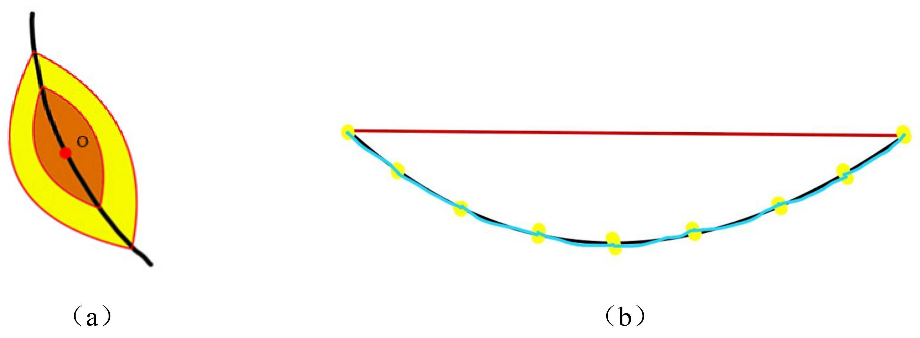
Fréchet distance is a path space similarity description proposed by French mathematician Fréchet which focuses on the path space distance and is more accurate and efficient in evaluating the similarity of curves with a certain spatial time order. This paper uses the Fréchet distance to measure the spatial similarity of two paths and determine whether the critical point is still located on the crack.
As shown in Figure 11, there are two paths in red and black, and the points of the same number amount are selected at equal distances on these two paths, respectively; the Euclidean distance between the corresponding points on the two paths, i.e., the length of the blue line segment in Figure 11, is calculated; and the maximum value of the length is taken as the Fréchet distance between the two paths. If this distance is less than the given threshold, then the two paths are considered to be spatially similar.
The path is denoted as M, and the path is denoted as N. Then, the paths M and N are point sequences with the same starting and ending points and consist of discrete points. To simplify the calculation, the number of points in the point sequence is used as the length of the path. Suppose that there are discrete points in M and discrete points in N. If a mapping is established between paths M and N, and the i-th point in path M corresponds to the point in path N, the Fréchet interval distance between the paths M and N is as follows:
where M(i) denotes the coordinates of the i-th point on path M, N(i) denotes the coordinates of the i-th point on path N, and d(x, y) denotes the Euclidean distance between x and y. Since path N is a sequence of points consisting of discrete points, the corresponding position estimate, N(i/m), is obtained by linear interpolation when is a non-integer.
If A, B, and C are on the crack, the following equation obviously holds:
Since the two paths cannot coincide exactly, the Fréchet distance between them is obviously greater than 0. Moreover, the number of discrete points in the path is generally not the same, and the coordinates of the corresponding points obtained by linear interpolation also have errors, resulting in the calculated Fréchet distance not being accurate enough; therefore, in the actual operation, the following equation is considered as the judgment condition for the end of the algorithm.
The determination of the Fréchet distance, , is simpler than the selection of in the triangular relationship, and it is only necessary to determine the range of Fréchet error according to the fluctuation amplitude, which is related to the crack width. In this paper, is set to the crack width, and the step parameter has no effect on it. Facing the difficult situation of the triangular relationship in Figure 10, the Fréchet distance can be solved well. The length of the blue line segment in Figure 10 is the Fréchet distance of the two paths. The spatial similarity of the paths is negatively correlated with the size of the Fréchet distance, and the larger the spatial correlation of the two paths, the smaller their Fréchet distance; thus, the Fréchet distance can be used as a simple method to judge the similarity of the paths.
2.2.3. Multiscale Pyramid Strategy
In the actual calculation, in this paper, we use a multiscale pyramid strategy to compress the image to one-half scale and one-quarter scale by filtering the pyramid and store these two layers together with the original image in an array for speedy retrieval. For the topmost image, first use the FMM algorithm to obtain the shortest path between the key point and the key point and pass it to the next layer. Then, find the shortest path between two adjacent key points in the second layer and calculate the Fréchet distance between this path and the shortest path in the first layer. If it is less than the set Fréchet distance threshold, the point in the new path is the key point, and then pass the three key points and two paths to the third layer; otherwise, pass these two key points into the endpoint number group. Find the shortest distance between two adjacent key points in the third layer and calculate the Fréchet distance between this path and the shortest path in the second layer. If this distance is less than the set Fréchet distance threshold, pass the two key points and the path between into the final key point array and path array; otherwise pass these two key points into the endpoint array and wait for the next FMM algorithm. The crack extraction algorithm of the top-level image is shown in Figure 12:
For the second-layer image, FMM is performed starting from the points in the endpoint array. The discovered key points and shortest paths are passed down to the next layer. In the third layer, the shortest path between adjacent key points is searched, and the Fréchet distance between this path and the shortest path in the second layer is calculated. If this distance is less than the set Fréchet distance threshold, the two key points and the path between them are added to the final key point and path arrays. Otherwise, these two key points are passed to the endpoint array for the next round of the FMM algorithm. The crack extraction algorithm for the second layer image is shown in Figure 13:
For the third-layer image, FMM is performed starting from the points in the endpoint array. The discovered key points and shortest paths are directly passed into the key point and shortest path arrays. Finally, the combination of all paths in the shortest path array is the crack, and, thus, the extraction of cracks is completed. The extracted results are shown in Figure 14.
Although the approximate outline of the crack is extracted in Figure 14a, it lacks detailed information and misses a part of the crack. In Figure 14b, the details of the crack are enriched, and the cracks that were not extracted in the top layer of the pyramid are supplemented. The crack in Figure 14c has the most detail and appears smooth, which represents the final contour of our crack extraction. Based on Figure 14c, the crack-filling algorithm can be used to extract a complete and accurate crack, and the final results of the extraction are shown in Figure 15.
2.3. Remote-Sensing Workflow Processing
In the remote-sensing workflow processing section, this article proposes and implements a convenient, cost-effective, and practical road inspection method that uses mobile devices such as smartphones to replace professional on-board road crack detection equipment. The method can detect and extract road cracks in real time, while obtaining accurate crack measurement results. Firstly, an improved YOLOv5 detection model improved by a lightweight network module was used to extract target boxes from continuously captured road surface images. Then, based on the internal and external parameters obtained from camera calibration, inverse perspective transformation was performed to convert oblique images into orthographic images. Subsequently, the article proposes a crack detection method based on saliency enhancement and Fréchet decision-making to quickly and accurately detect and measure cracks in the corrected projection crack images. A complete remote-sensing processing workflow is provided for real-time road defect detection, ranging from mobile data acquisition to automated saliency detection of lane cracks.
2.3.1. Improved YOLOv5
It is described that mobile devices mounted on moving vehicles can obtain video data of the road ahead after being adjusted to an appropriate angle. For convenience in subsequent experiments, the data are first preprocessed by slicing, and then crack detection and rough positioning are performed using a deep-learning object detection network.
The improved YOLOv5 road crack detection model used in this study was designed for mobile devices with limited computing resources, which can achieve fast prediction speed during network model inference on mobile CPUs such as smartphones. The YOLO series neural network is a one-stage object detection algorithm that divides the input image into n×n grids; generates two initial prior boxes with different aspect ratios, using the center of each grid as the anchor point; and binds the prior boxes with ground-truth boxes to calculate bounding box regression loss, classification loss, and confidence loss. It applies Non-Maximum Suppression (NMS) to eliminate overlapping detection boxes and outputs the resulting detection boxes that exceed the given confidence threshold and IOU threshold, including the pixel coordinates of the detection boxes, the road cracks, and the confidence of the detection results.
The modifications made to the YOLOv3 [38] model for YOLOv5 mainly include using Mosaic augmentation during preprocessing to perform adaptive image scaling; adding Cross-Stage Partial (CSP) structures with residual connections in the backbone network to maintain accuracy, while reducing parameters; improving Spatial Pyramid Pooling (SPP) on the basis of the neck network to further solve the problem of multiscale targets; adopting the Path Aggregation Network (PAN) module to add a bottom-up route to compensate for detailed information; and using the CIoU loss function in the head network to more effectively filter detection results and improve the accuracy of the network [39].
Using a lightweight model structure to extend the YOLOv5 network can not only ensure that the overall network structure is not broken but also achieve model compression and acceleration with less time cost and resource cost, without a well-trained large model. PP-LCNet is a unique high-performance backbone network customized for Intel CPU environments based on the current industry situation in the Baidu PaddleClass image classification suite. Under the same precision, its speed far exceeds current backbone networks based on CPUs such as MobileNetV2 [40], ShuffleNetV2 [41], etc. Applied in target detection, semantic segmentation, and other algorithm tasks, it can significantly improve the performance of the original network. The basic structure of PP-LCNet is shown in Figure 16.
The article removes the global average pooling layer and its subsequent fully connected layer in PP-LCNet, replaces the backbone network of YOLOv5s; inputs 8-, 16-, and 32-times down-sampled feature maps into the neck network of YOLOv5; and finally outputs to the head prediction network to obtain detection results. The 8× and 32× down-sampling layers of PP-LCNet only undergo the next down-sampling after the DepthSepConv-1 module, resulting in limited feature extraction capabilities, making it difficult for the model to merge high- and low-level feature maps in the neck network. Therefore, we attempted to add two DepthSepConv-1 modules with a stride of 1-time after 8-times down-sampling and two DepthSepConv-2 modules with a stride of 2- after 32-times down-sampling to improve the feature extraction performance of the backbone network. The improved YOLOv5 network is called PP-LCNet-YOLOv5, and its structure is shown in Figure 17.
2.3.2. Perspective Inversion Transformation
Before performing the inverse perspective transformation on the rectangular boxes detected by improved YOLOv5, it is necessary to calibrate the camera that captured the images. The calibration method used in this study is Zhang’s calibration method, which fixes the world coordinate system on the checkerboard. That is, the world coordinates of any point on the checkerboard are Z = 0. Since the world coordinates system of the calibration board is defined beforehand, and the size of each cell on the calibration board is known, the physical coordinates of each corner point on the checkerboard in the world coordinate system are (X, Y, 0). Suppose the image coordinates of the checkerboard corner points are (u, v). If the camera intrinsic parameters are A, the rotation matrix of a certain photo is R, and the translation matrix is T, then according to the camera imaging model, each corner point on the checkerboard satisfies the following Equation (13):
By eliminating the scale factor, Z, we can obtain the following:
When the number of calibration board corner points on an image is greater than or equal to 4, matrix H can be calculated. When there are more than 3 images of the checkerboard, it can provide us with enough constraints to solve the camera’s intrinsic and extrinsic parameters from matrix H. Assuming that the road surface is flat, we can perform inverse perspective transformation, using the camera’s intrinsic parameters, three attitude angles (pitch angle, yaw angle, and roll angle), and extrinsic parameters. First, a world coordinate system, a camera coordinate system, and an image coordinate system are defined as shown in Figure 18.
We allow the camera to have a roll angle (γ), pitch angle (α), and yaw angle (β); that is, the attitude of the camera is free, the height of the camera above the ground is h, and the homogeneous transformation matrix, , can be obtained from the camera model. Starting from any point, , on the image, the projection point of this point on the ground can be found by applying and as shown below:
In the matrix, and are the horizontal and vertical focal lengths of the camera, respectively; are the image coordinate system of the optical center of the camera; and , , , , , and . The projection points of the four vertices, , of the input rectangle on the road plane can be calculated by the formula , and then the isomorphic part needs to be scaled. From this perspective, the rectangle on the image will become a trapezoid on the road plane. The inverse transformation of the transform, , is as follows:
Starting at a point, , on the road plane, apply the pass formula, . The subpixel coordinates on the image frame corresponding to the point can be inversely calculated, and the isomorphic part also needs to be scaled. Using the above two transformations, the input rectangle box can be projected onto the road plane. The schematic diagram of IPM transformation is shown in Figure 18.
3. Results
3.1. Dataset
The dataset for this paper is divided into two parts, the public dataset and the self-collected dataset, respectively. The public dataset is mainly used for training and testing YOLOv5 networks. The self-collected dataset is the road image collection conducted by the author’s team around Huanshan North Road and Fengyuan Road in Wuhan University. The training dataset that was used for training and improved the YOLOv5 network is Road Damage Detection-2020 (RDD-2020), which contains 26,620 images collected from three countries: India, Japan, and the Czech Republic. There are four common damage types: longitudinal crack (D00), transverse crack (D10), crack (D20), and pothole (D40). In this study, the original training set was divided into a training set and a test set in a ratio of about 9:1. The improved YOLOv5 code proposed in this paper was run under the deep-learning framework of Python3.8, Pytorch1.8, and cuda11.0, and the model was trained and tested on the NVIDIA 3080 Ti graphics card with 12 GB video memory. Random gradient descent (SGD) optimization was adopted in this study. The initial learning rate was set as 0.01, the momentum coefficient was set as 0.937, the weight attenuation was set as 0.0005, and the learning rate adjustment strategy of cosine annealing was used. The total number of training epochs was set as 300. The batch size was set to 40–80 depending on the model size. The training data were enhanced by mosaic and then input to the network. The input image size was 640 × 640 during training and 640 × 640 during the test.
In order to evaluate the effect of the method proposed in this paper, a family car equipped with a HUAWEI P30 mobile phone was used to collect road-image data on Huanshan North Road and Fengyuan Road of Wuhan University, Wuchang District, Wuhan City, Hubei Province. The route is shown in Figure 19. The whole experiment covered about 20 km of road mileage, and then we extracted images frame by frame. A total of 14,520 images of road surface condition were collected, with a resolution of 720 × 1280. The types of cracks in the image include longitudinal cracks, transverse cracks, and cracks. There are various scenes in the image, including a variety of straight roads and detours. The road condition is complex; there are interferences such as oil and foreign bodies on the road surface, uneven illumination of the image, cracks in crosswalks, and so on. These complex conditions may affect the accuracy of crack extraction. This paper firstly takes a typical crack as an example to give the data-processing results of each stage and the final fracture extraction results; it then gives the results of the algorithm extraction of different types of cracks and crack extraction results under complex background conditions; and, finally, it carries out the accuracy evaluation and error analysis.
3.2. Evaluation Index
To evaluate the accuracy of the road-sign detection algorithm in this article, the total number of road signs, as extracted by the algorithm, is compared with the manually counted number of road signs, and the accuracy and recall rates are calculated using the following equation:
In the formula, true positive (TP) represents the number of pixels detected by the algorithm as cracks, but not as cracks in the actual ground values. False positive (FP) represents the number of pixels detected by the algorithm as cracks, but not as cracks in the ground truth. False negative (FN) represents the number of pixels detected by the algorithm as non-crack, but in the ground truth, they are cracks.
Therefore, precision and recall are used to quantify the number of correct detections that actually belong to cracks, and these predictions are composed of all detection results in the dataset. provides a single score that balances the issues of accuracy and recalls in a single number. If crack detection meets high accuracy, recall, and values simultaneously, then it is indeed a good method.
Due to the complexity of road surface images, manually marked ground-truth values may produce deviations. Therefore, when measuring the coincidence between the detected crack curve and the ground-truth crack curve, we allow a certain tolerance. More specifically, if the detected crack pixel is no more than 1 pixel from the real crack curve on the ground, it is still considered the correct detected pixel.
3.3. Typical Situation
This section uses a typical road image as an example to illustrate the data-processing results of each stage of crack extraction. In order to facilitate the subsequent inverse perspective transformation, it is necessary to perform Zhang Youzheng calibration before processing. Figure 20 shows some of the checkerboard images used during the calibration.
In order to obtain the height of the camera relative to the ground and the Euler angle of the camera, it is necessary to calibrate the checkerboard placed flat on the ground. The image set used is shown in Figure 21.
After calibration, the rotation matrix of the camera can be obtained as follows:
The translation matrix of the camera is as follows:
According to the rotation matrix and translation matrix of the camera, the height of the camera is , the camera’s , the camera’s , and the camera’s , which can be substituted into the IPM change matrix to obtain the following:
The inverse of this change is as follows:
Using these two matrices, an inverse perspective transformation can be performed on the image.
Figure 22a is an image of a certain frame selected in the video. It can be seen that there are not only cracks in the original image but also the interference of pedestrians and various backgrounds. To focus on the cracks, we used the trained YOLOv5 network to perform rough positioning of the ROI on Figure 22a, and the positioning result is shown in Figure 22b. The results of the proposed method, PP-LCNet-YOLOv5, in this article are shown in Figure 22c. Compared to the original YOLOv5, the coarse localization method used in this article improved positioning accuracy and completeness. The DepthSepConv-1 module added in PP-LCNet-YOLOv5 improved the feature extraction performance of the network. The mAP of YOLOv5 is 78.9%. However, the mAP of PP-LCNet-YOLOv5 is 84.5%. Afterward, inverse perspective transformation, saliency enhancement, and crack extraction were performed on the area, and the result is shown in Figure 23.
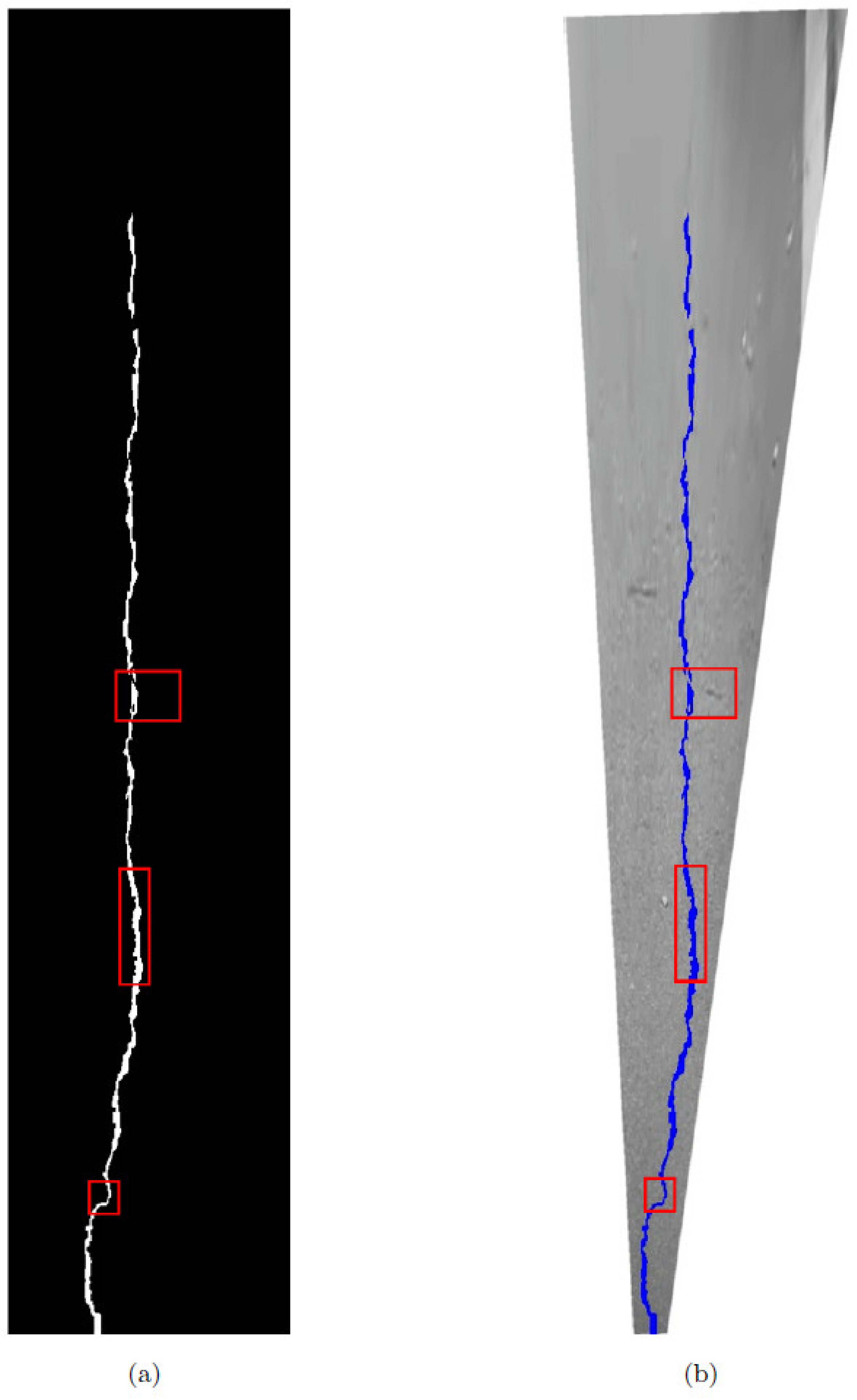
It can be seen that after the significance enhancement, the cracks are now very obvious and can be distinguished from the background, but there are still external noises, background points inside the cracks, and discontinuous cracks, as indicated by the red box in Figure 23. It is shown that the next step is to use the fast-marching method to further extract the fractures. To be able to start the fast-marching method, one needs to select a point as the starting point of the algorithm. We started the fast-marching method with the most significant point at the 5 pixels inside the IPM box as the starting point. In the process of searching for key points, we used the triangle relationship improved by the Fréchet distance as the criterion for the termination of the fast-marching method; the extracted cracks are shown in Figure 24.
From the blue frame in Figure 24, we can see that the extracted cracks have eliminated the interference of external noise, the inside of the cracks is also very continuous, and the two intermittent cracks on the salient image are now connected into one. Generally speaking, the crack extraction is more accurate, and the misjudgment rate is lower. The above effect could be achieved because the joint processing method of saliency image and Fréchet distance was adopted in this study. Figure 25 shows the most original results, using only saliency image results and results using only the F-distance.
It can be seen from Figure 25 that using the F-distance criterion can increase the accuracy of crack judgment and reduce the misjudgment caused by the Euclidean distance criterion, as shown in the red box at the bottom of Figure 25a,b. The use of saliency enhancement can make the inconspicuous cracks obvious, which helps to extract them and separate them from the background, as shown in the upper red box in Figure 25a,b. Combining the F-distance criterion and the significance enhancement, the advantages of the two can be combined to extract the cracks with the best effect. According to the statistics, the length of the crack on the image is 2484 pixels. When an inverse perspective transformation is performed, sampling is performed every 2 mm, meaning that the actual distance represented by each pixel is 2 mm, so the actual length of the crack is 4.968 m, which is very close to the crack length we measured on the spot, i.e., 4.98 m, thus showing that the method in this paper is accurate.
3.4. Overall Results
To verify the performance of the method in this paper, taking the three common shapes of cracks—longitudinal cracks (a), transverse cracks (b), and cracks (c)—as examples, the results of inverse perspective transformation and saliency calculation are shown, as well as the effect of crack extraction, the effect superimposed on the original image and the shape attribute of the crack.
For the crack shown in Figure 26a, its extension direction is perpendicular to the direction of travel of the car; it is called a transverse crack. Using the algorithm in this paper, the cracks in the graph can be accurately extracted. This image was collected on a road close to flat ground, and it is at the beginning of data collection, so the inverse perspective transformation has high accuracy. According to our algorithm, the crack length calculated is 3.942 m, and the actual crack length is 4.015 m. The error is 0.072 m.
For the crack shown in Figure 27b, its extension direction is the same as the direction of travel of the car, and it is called a longitudinal crack. Accurate and complete cracks can still be extracted using the algorithm in this paper. This image was collected on an uphill road. During the uphill process, the mobile phone fixed on the car may be slightly disturbed, which will affect the result of the inverse perspective transformation to a certain extent, which is reflected in the incomplete lane in the inverse perspective image. Perpendicular to the bottom of the photo. Figure 28 is the result of processing longitudinal cracks by the algorithm proposed in this paper. It can be seen that the algorithm in this paper can extract complete and continuous longitudinal cracks. The fracture length calculated according to the algorithm in this paper is 6.326 m, the actual length of the fracture is 6.201 m, and the error is 0.125 m.
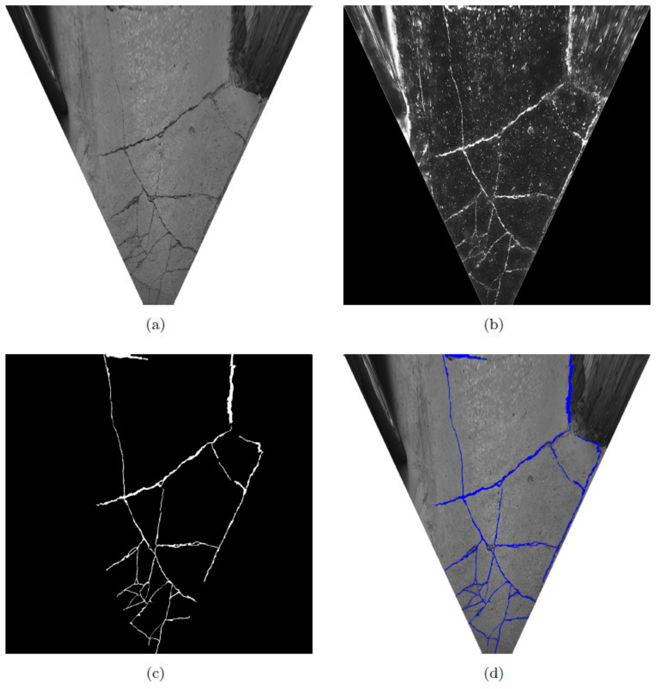
Figure 28 shows the results of each stage of crack extraction in Figure 26a. It can be seen that the cracks in the original image are not obvious. After the significance enhancement, the cracks and the background were clearly distinguished, but not continuous enough. After being processed by the FMM algorithm, continuous and complete fractures were extracted. As shown in Figure 28c, the crack has no fixed extension direction and has a turtle-shell-like pattern. This type of crack has the greatest impact on the road and is prone to evolve into potholes, posing a significant safety hazard to drivers. Due to its irregular shape, extracting it is challenging. The result of using the method proposed in this paper to extract the crack is shown in Figure 29. As it is difficult to accurately measure the total length of the turtle-shell-like crack, only the crack in the blue box in Figure 30d was measured. The crack length calculated by our algorithm was 1.675 m, while the actual length of the crack was 1.613 m, resulting in an error of 0.062 m.
After statistical calculation, the average error in calculating the length of cracks is 0.127 m, and the average length of cracks is 4.68 m. The relative error in calculating the length of the method proposed in this article is 3%, which is an acceptable range of error. The same evaluation method was used for Reference [42], with a relative accuracy of 5.3%. This indicates that the algorithm proposed in this article is a very accurate remote-sensing method.
3.5. Complex Conditions
The method proposed in this paper was also tested on road images with complex backgrounds. These images were relatively blurry and were affected by factors such as shadows, noise, and non-uniform lighting. For each scenario, we enhanced the saliency image and then used the fast-marching method to extract the cracks. The extraction results are shown below.
As road images are collected from asphalt pavement, they inevitably mix with many lane markings, as shown in Figure 30. The lane markings are pure white, and their edges have a sudden change in grayscale value where they meet the road surface. Edge-based crack detection algorithms can easily mistake these edges for crack edges. However, the method presented in this paper detects cracks using saliency enhancement, which is not affected by lane markings.
About half of the road surface image shown in Figure 30 is covered by shadows. Compared to the area with sufficient lighting, the gray value of the background in the shadow area is approximate to the gray value of the cracks. If cracks are extracted directly, this may lead to inaccurate extraction results. First, using saliency enhancement can enhance the contrast between the cracks and the background. By extracting cracks on the saliency image, better results can be extracted.
3.6. Accuracy Evaluation and Error Analysis
This study selected the fast-marching method, only using saliency, and only using F-distance to compare the accuracy, recall, and F1 measure evaluation indicators of the proposed method. The comparison results are shown in the Table 1 and the Figure 31, indicating that this article has certain advantages in all three indicators.
Although the method presented in this paper can extract most of the cracks, there are still cases where foreign objects on the ground are recognized as cracks by the improved YOLOv5 network. As shown in Figure 32, it may detect foreign objects on the ground, such as manhole covers, as cracks (Figure 32a), and it may mistake leaves as horizontal or vertical cracks (Figure 32a–c). The algorithm proposed in this paper cannot exclude such foreign objects on the ground that are highly similar to cracks in both shape and texture. It is recommended to further remove false positives based on more detailed terrain recognition.
4. Conclusions
Lane cracks are one of the biggest threats to road conditions. The automatic detection of lane cracks can not only assist in evaluating road quality but also be used to develop the best crack repair plan, thereby maintaining road smoothness and ensuring driving safety. Although cracks can be extracted from road images due to their lower pixel grayscale intensity than the background grayscale intensity, extracting continuous and complete cracks from complex-texture, high-noise, and uneven-lighting lane images remains a challenge. Although the significance enhancement method can distinguish cracks from the background, the extracted cracks are discontinuous and cannot exclude the influence of noise. Although the fast-marching method can extract continuous cracks, it has the problem of “taking shortcuts” and is prone to extracting incorrect cracks under complex lighting conditions. This study innovatively used a saliency enhancement method to enhance the image, introducing Fréchet distance to solve the problems of the fast-marching method, and created a complete remote-sensing process that can collect crack images and calculate crack attributes, using low-cost equipment. This study first used the improved YOLOv5 network to roughly locate the crack ROI in the collected image, then performed an inverse perspective transformation on the crack ROI to generate a top view image, and then enhanced the saliency of the image to generate a saliency image. Finally, the fast-marching method that introduced the Fréchet distance was used to extract the crack. Due to the fact that the corresponding relationship between pixel distance and actual distance was determined during inverse perspective transformation, the actual distance of cracks can be obtained by counting the number of pixels of cracks in the image. This can help us determine the actual width and length of cracks and evaluate the damage situation of the road surface.
This study used a household car equipped with a fixed-posture mobile phone to collect road image data on Huanshan North Road and Fengyuan Road in Wuchang District, Wuhan City, Hubei Province. The experimental data cover about 20 km of road mileage, and a total of 14,520 road surface image data were collected. The cracks have complex shapes, including longitudinal cracks, transverse cracks, and cracking cracks. The road conditions where the cracks are located are diverse, with various complex conditions such as uneven lighting and noise from sidewalks and asphalt roads. A large number of experiments on real road images have shown that the algorithm proposed in this paper can achieve crack extraction with an accuracy of 89.3%, a recall rate of 87.1%, and an F1 value of 88.2% and can calculate the length and width of cracks. The algorithm proposed in this article is expected to be applied to road departments in various provinces and cities, assisting in evaluating road quality and specifying the optimal crack repair plan. Although the method proposed in this article can solve most of the problems of pavement crack detection, further in-depth research is still needed regarding the following two aspects. Firstly, for the discontinuity problem in some crack results, further continuity processing is needed to identify the cracks as complete target objects with independent features. Secondly, YOLOv7 is used to locate the location of cracks. When training the network, it is necessary to pay attention to the balance of positive and negative samples and try to increase the proportion of crack images in the overall sample as much as possible, so that the training network can more effectively locate cracks.
Author Contributions
S.Z., G.L. and A.L. conceived and conducted the experiments and performed the data analysis. S.Z. wrote the article. S.Z. and Z.F. revised the manuscript. All authors have read and agreed to the published version of the manuscript.
Funding
This research received no external funding.
Data Availability Statement
Not applicable.
Acknowledgments
We would like to thank the anonymous reviewers for their constructive and valuable suggestions on the earlier drafts of this manuscript.
Conflicts of Interest
The authors declare no conflict of interest.
References
- Chen, Q.; Huang, Y.; Sun, H.; Huang, W. Pavement crack detection using hessian structure propagation. Adv. Eng. Inform. 2021, 49, 101303. [Google Scholar] [CrossRef]
- Zhang, H.; Huang, C.C. Intelligent thinking of rural road maintenance decision. China Highw. 2021, 20, 74–77. [Google Scholar]
- Amila, A.; Emir, B.; Samir, O.; Almir, K. Pavement crack detection using Otsu thresholding for image segmentation. In Proceedings of the 2018 41st International Convention on Information and Communication Technology, Electronics and Microelectronics (MIPRO), Opatija, Croatia, 21–25 May 2018; pp. 1092–1097. [Google Scholar]
- Quan, Y.; Sun, J.; Zhang, Y.; Zhang, H. The Method of the Road Surface Crack Detection by the Improved Otsu Threshold. In Proceedings of the 2019 IEEE International Conference on Mechatronics and Automation (ICMA), Tianjin, China, 4–7 August 2019; pp. 1615–1620. [Google Scholar]
- Luo, Q.; Ge, B.; Tian, Q. A fast adaptive crack detection algorithm based on a double-edge extraction operator of FSM. Constr. Build. Mater. 2019, 204, 244–254. [Google Scholar] [CrossRef]
- Huyan, J.; Li, W.; Tighe, S.; Xiao, L.; Sun, Z.; Shao, N. Three-dimensional pavement crack detection based on primary surface profile innovation optimized dual-phase computing. Eng. Appl. Artif. Intell. 2020, 89, 103376. [Google Scholar] [CrossRef]
- Huan, X.; Li, Z.; Jiang, Y.; Huang, J. Pavement crack detection based on OpenCV and improved Canny operator. Eng. Design 2014, 35, 4254–4258. [Google Scholar]
- Othman, Z.; Abdullah, A.; Kasmin, F.; Ahmad, S.S.S. Road crack detection using adaptive multi resolution thresholding techniques. TELKOMNIKA 2019, 17, 1874. [Google Scholar] [CrossRef]
- Achanta, R.; Estrada, F.; Wils, P.; Süsstrunk, S. Salient region detection and segmentation. In Proceedings of the Computer Vision Systems: 6th International Conference, ICVS 2008, Santorini, Greece, 12–15 May 2008; Proceedings 6. Springer: Berlin/Heidelberg, Germany, 2008; pp. 66–75. [Google Scholar]
- Kass, M.; Witkin, A.; Terzopoulos, D. Snakes: Active contour models. Int. J. Comput. Vis. 1988, 1, 321–331. [Google Scholar] [CrossRef]
- Sethian, J.A. A fast marching level set method for monotonically advancing fronts. Proc. Nat. Acad. Sci. USA 1995, 93, 1591–1595. [Google Scholar] [CrossRef]
- Amhaz, R.; Chambon, S.; Idier, J.; Baltazart, V. Automatic Crack Detection on Two-Dimensional Pavement Images: An Algorithm Based on Minimal Path Selection. IEEE Trans. Intell. Transp. Syst. 2016, 17, 2718–2729. [Google Scholar] [CrossRef]
- Amhaz, R.; Chambon, S.; Idier, J.; Baltazart, V. A new minimal path selection algorithm for automatic crack detection on pavement images. In Proceedings of the 2014 IEEE International Conference on Image Processing (ICIP), Paris, France, 27–30 October 2014; pp. 788–792. [Google Scholar]
- Nguyen, T.S.; Begot, S.; Duculty, F.; Avila, M. Free-form anisotropy: A new method for crack detection on pavement surface images. In Proceedings of the 2011 18th IEEE International Conference on Image Processing, Brussels, Belgium, 11–14 September 2011; pp. 1069–1072. [Google Scholar]
- Kaddah, W.; Elbouz, M.; Ouerhani, Y.; Baltazart, V.; Desthieux, M.; Alfalou, A. Optimized minimal path selection (OMPS) method for automatic and unsupervised crack segmentation within two-dimensional pavement images. Vis. Comput. 2019, 35, 1293–1309. [Google Scholar] [CrossRef]
- Zhou, Y.; Wang, F.; Meghanathan, N.; Huang, Y. Seed-Based Approach for Automated Crack Detection from Pavement Images. Transp. Res. Rec. 2016, 2589, 162–171. [Google Scholar] [CrossRef]
- Balasubramaniam, K.; Sikdar, S.; Ziaja, D.; Jurek, M.; Soman, R.; Malinowski, P. A global-local damage localization and quantification approach in composite structures using ultrasonic guided waves and active infrared thermography. Smart Mater. Struct. 2023, 32, 35016. [Google Scholar] [CrossRef]
- Hsieh, Y.; Tsai, Y.J. Machine Learning for Crack Detection: Review and Model Performance Comparison. J. Comput. Civ. Eng. 2020, 34, 04020038. [Google Scholar] [CrossRef]
- Joseph, R.; Santosh, D.; Ross, G.; Ali, F. You only look once: Unified real-time object detection. In Proceedings of the 2016 IEEE Conference on Computer Vision and Pattern Recognition (CVPR), Las Vegas, NV, USA, 27–30 June 2016; pp. 779–788. [Google Scholar]
- Ma, D.; Fang, H.; Wang, N.; Zhang, C.; Dong, J.; Hu, H. Automatic Detection and Counting System for Pavement Cracks Based on PCGAN and YOLO-MF. IEEE Trans. Intell. Transp. Syst. 2022, 23, 22166–22178. [Google Scholar] [CrossRef]
- Glenn, J.; Alex, S.; Jirka, B.; Ayush, C.; Tao, X.; Liu, C. ultralytics/yolov5: v5.0—YOLOv5-P6 1280 Models AWS Supervise.ly and YouTube Integrations. 2021. Available online: https://ui.adsabs.harvard.edu/abs/2021zndo...4679653J/abstract (accessed on 15 August 2023).
- Sha, A.; Tong, Z.; Gao, J. Road surface disease recognition and Measurement based on Convolutional neural networks. China J. Highw. Transp. 2018, 31, 1–10. [Google Scholar]
- Hoang, N.-D. An artificial intelligence method for asphalt pavement pothole detection using least squares support vector machine and neural network with steerable filter-based feature extraction. Adv. Civ. Eng. 2018, 2018, 7419058. [Google Scholar] [CrossRef]
- Wang, L.; Zhuang, L.; Zhang, Z. Automatic detection of rail surface cracks with a superpixel-based data-driven framework. J. Comput. Civ. Eng. 2018, 33, 4018053. [Google Scholar] [CrossRef]
- Shi, Y.; Cui, L.; Qi, Z.; Meng, F.; Chen, Z. Automatic road crack detection using random structured forests. IEEE Trans. Intell. Transp. Syst. 2016, 17, 3434–3445. [Google Scholar] [CrossRef]
- Peng, C.; Yang, M.; Zheng, Q.; Zhang, J.; Wang, D.; Yan, R.; Wang, J.; Li, B. A triple thresholds pavement crack detection method leveraging random structured forest. Constr. Build. Mater. 2020, 263, 120080. [Google Scholar] [CrossRef]
- Li, G.; Zhao, X.; Du, K.; Ru, F.; Zhang, Y. Recognition and evaluation of bridge cracks with modified active contour model and greedy search-based support vector machine. Autom. Constr. 2017, 78, 51–61. [Google Scholar] [CrossRef]
- Wang, S.; Qiu, S.; Wang, W.; Xiao, D.; Wang, K.C.P. Cracking classification using minimum rectangular cover–based support vector machine. J. Comput. Civ. Eng. 2017, 31, 4017027. [Google Scholar] [CrossRef]
- Chen, F.-C.; Jahanshahi, M.R.; Wu, R.-T.; Joffe, C. A texture-based video processing methodology using Bayesian data fusion for autonomous crack detection on metallic surfaces. Comput.-Aided Civ. Infrastruct. Eng. 2017, 32, 271–287. [Google Scholar] [CrossRef]
- Ai, D.; Jiang, G.; Kei, L.S.; Li, C. Automatic pixel-level pavement crack detection using information of multi-scale neighborhoods. IEEE Access. 2018, 6, 24452–24463. [Google Scholar] [CrossRef]
- Yuan, G.; Li, J.; Meng, X.; Li, Y. CurSeg: A pavement crack detector based on a deep hierarchical feature learning segmentation framework. IET Intell. Transp. Syst. 2022, 16, 782–799. [Google Scholar] [CrossRef]
- Wu, F.Y.; Yang, Z.; Mo, X.K.; Wu, Z.H.; Tang, W.; Duan, J.L.; Zou, X.J. Detection and counting of banana bunches by integrating deep learning and classic image-processing algorithms. Comput. Electron. Agric. 2023, 209, 0168–1699. [Google Scholar] [CrossRef]
- Zhou, T.H.; Tang, Y.H.; Zou, X.J.; Wu, M.L.; Tang, W.; Meng, F.; Zhang, Y.Q.; Kang, H.W. Adaptive Active Positioning of Camellia oleifera Fruit Picking Points: Classical Image Processing and YOLOv7 Fusion Algorithm. Appl. Sci. 2022, 12, 12959. [Google Scholar] [CrossRef]
- Tang, Y.; Chen, Z.; Huang, Z.; Nong, Y.; Li, L. Visual measurement of dam concrete cracks based on U-net and improved thinning algorithm. J. Exp. Mech. 2022, 37, 209–220. [Google Scholar]
- Tang, Y.; Huang, Z.; Chen, Z.; Chen, M.; Zhou, H.; Zhang, H.; Sun, J. Novel visual crack width measurement based on backbone double-scale features for improved detection automation. Eng. Struct. 2023, 274, 115158. [Google Scholar] [CrossRef]
- Chang, B.R.; Tsai, H.F.; Hsieh, C.W. Location and timestamp-based chip contour detection using LWMG-YOLOv5. Comput. Ind. Eng. 2023, 180, 109277. [Google Scholar] [CrossRef]
- Kichenassamy, S.; Kumar, A.; Olver, P.; Tannenbaum, A.; Yezzi, A. Gradient Flows and Geometric Active Contour Models. In Proceedings of the IEEE International Conference on Computer Vision, Cambridge, MA, USA, 20–23 June 1995. [Google Scholar]
- Joseph, R.; Ali, F. Yolov3: An incremental improvement. arXiv 2018, arXiv:1804.02767. [Google Scholar]
- Cui, C.; Gao, T.; Wei, S.; Du, Y.; Guo, R.; Dong, S.; Lu, B.; Zhou, Y.; Lv, X.; Liu, Q.; et al. PP-LCNet: A Lightweight CPU Convolutional Neural Network. arXiv 2021, arXiv:2109.15099. [Google Scholar]
- Sandler, M.; Howard, A.; Zhu, M.; Zhmoginov, A.; Chen, L.-C. MobileNetV2: Inverted Residuals and Linear Bottlenecks. In Proceedings of the 2018 IEEE/CVF Conference on Computer Vision and Pattern Recognition (CVPR), Salt Lake City, UT, USA, 18–23 June 2018; pp. 4510–4520. [Google Scholar]
- Ma, N.; Zhang, X.; Zheng, H.T.; Sun, J. Shufflenet v2: Practical guidelines for efficient cnn architecture design. In Proceedings of the European Conference on Computer Vision (ECCV), Munich, Germany, 8–14 September 2018; pp. 116–131. [Google Scholar]
- Fei, Y.; Wang, K.C.; Zhang, A.; Chen, C.; Li, J.Q.; Liu, Y.; Yang, G.; Li, B. Pixel-level cracking detection on 3D asphalt pavement images through deep-learning-based CrackNet-V. IEEE Trans. Intell. Transp. Syst. 2019, 21, 273–284. [Google Scholar] [CrossRef]
Figure 1.
Remote-sensing process diagram of crack extraction based on the significance.

Figure 2.
Valley structure of cracks. (a) Obvious valley structure. (b) Indistinct valley structure.
Figure 2.
Valley structure of cracks. (a) Obvious valley structure. (b) Indistinct valley structure.

Figure 3.
Significance test window.

Figure 4.
Saliency test on the image. (a) The saliency test window on the image. (b) The grayscale probability distribution of pixel x.
Figure 4.
Saliency test on the image. (a) The saliency test window on the image. (b) The grayscale probability distribution of pixel x.

Figure 5.
Transverse crack.

Figure 6.
Crack image after saliency enhancement.

Figure 7.
Comparison between FMM algorithm and Dijkstra algorithm. (a) Dijkstra algorithm, the distance d(x) is updated by d(x1). (b) FMM algorithm, the distance d(x) is updated based on d(x1), d(x2), and the relative relationships between x0, x1, and x2.
Figure 7.
Comparison between FMM algorithm and Dijkstra algorithm. (a) Dijkstra algorithm, the distance d(x) is updated by d(x1). (b) FMM algorithm, the distance d(x) is updated based on d(x1), d(x2), and the relative relationships between x0, x1, and x2.

Figure 8.
(a) Search direction of FMM algorithm. (b) The problem of taking shortcuts in FMM algorithm.
Figure 8.
(a) Search direction of FMM algorithm. (b) The problem of taking shortcuts in FMM algorithm.

Figure 9.
Diagram of triangular relationships. (a) All critical points on the crack. (b) A critical point appears off the crack.
Figure 9.
Diagram of triangular relationships. (a) All critical points on the crack. (b) A critical point appears off the crack.

Figure 10.
Examples of problems with triangulation. (a) Example 1 of the influence of step size parameters on the amplitude and frequency of the shortest path shift. (b) Example 2 of the influence of step size parameters on the amplitude and frequency of the shortest path shift. (c) Example 3 of the relationship between path length and actual crack length. (d) Example 3 of the relationship between path length and actual crack length.

Figure 11.
Fréchet distance diagram.

Figure 12.
Flowchart of the top-level FMM algorithm.

Figure 13.
Flowchart of the second-layer FMM algorithm.

Figure 14.
The results of crack extraction for each layer of the image pyramid are shown. (a) Compressed to 1/4 size. (b) Compressed to 1/2 size. (c) Original size.
Figure 14.
The results of crack extraction for each layer of the image pyramid are shown. (a) Compressed to 1/4 size. (b) Compressed to 1/2 size. (c) Original size.

Figure 15.
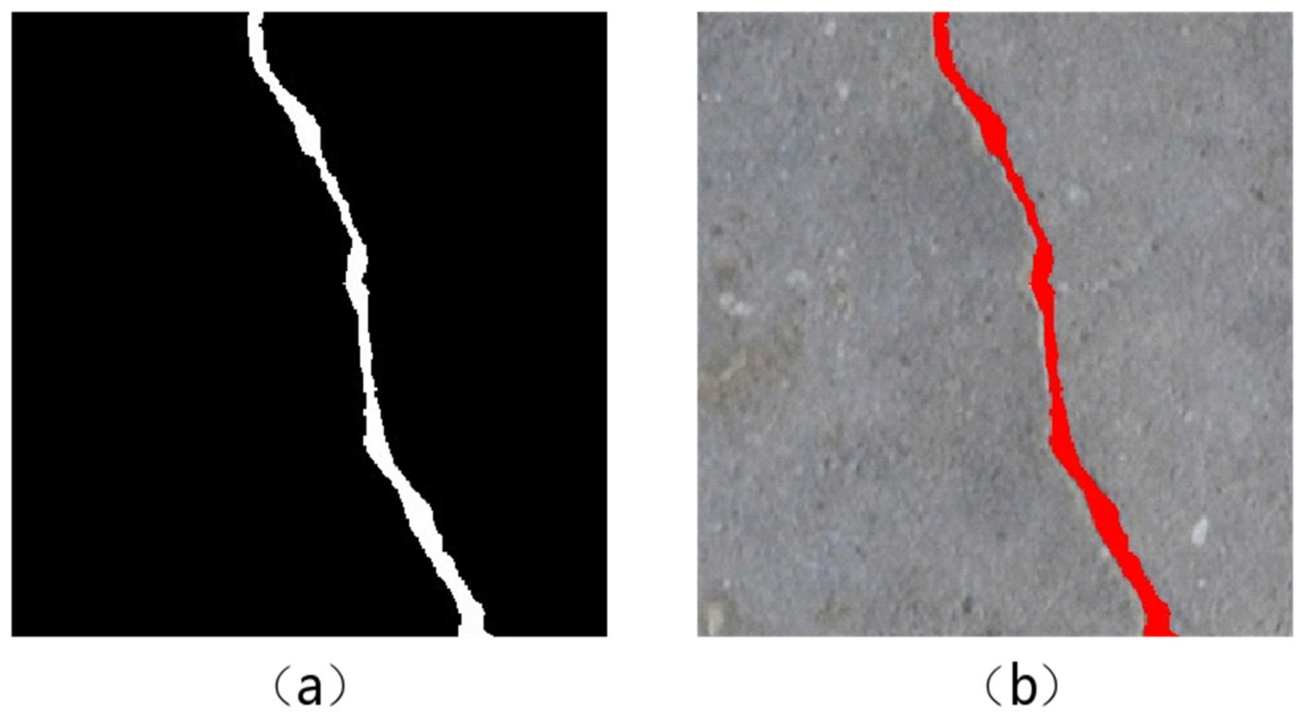
The final results of crack extraction. (a) The crack image. (b) The overlay of the crack and original image.
Figure 15.
The final results of crack extraction. (a) The crack image. (b) The overlay of the crack and original image.

Figure 16.
PP-LCNet network architecture.

Figure 17.
PP-LCNet-YOLOv5 network architecture.

Figure 18.
Image acquisition device and four coordinate systems.

Figure 19.
Experimental data-collection route.

Figure 20.
Checkerboard image set.

Figure 21.
Partial tessellation image set laid flat on the ground.

Figure 22.
Comparison of crack coarse positioning results. (a) The original image collected by the mobile phone. (b) The longitudinal crack extracted by YOLO. (c) The longitudinal crack extracted by PP-LCNet-YOLOv5.
Figure 22.
Comparison of crack coarse positioning results. (a) The original image collected by the mobile phone. (b) The longitudinal crack extracted by YOLO. (c) The longitudinal crack extracted by PP-LCNet-YOLOv5.

Figure 23.
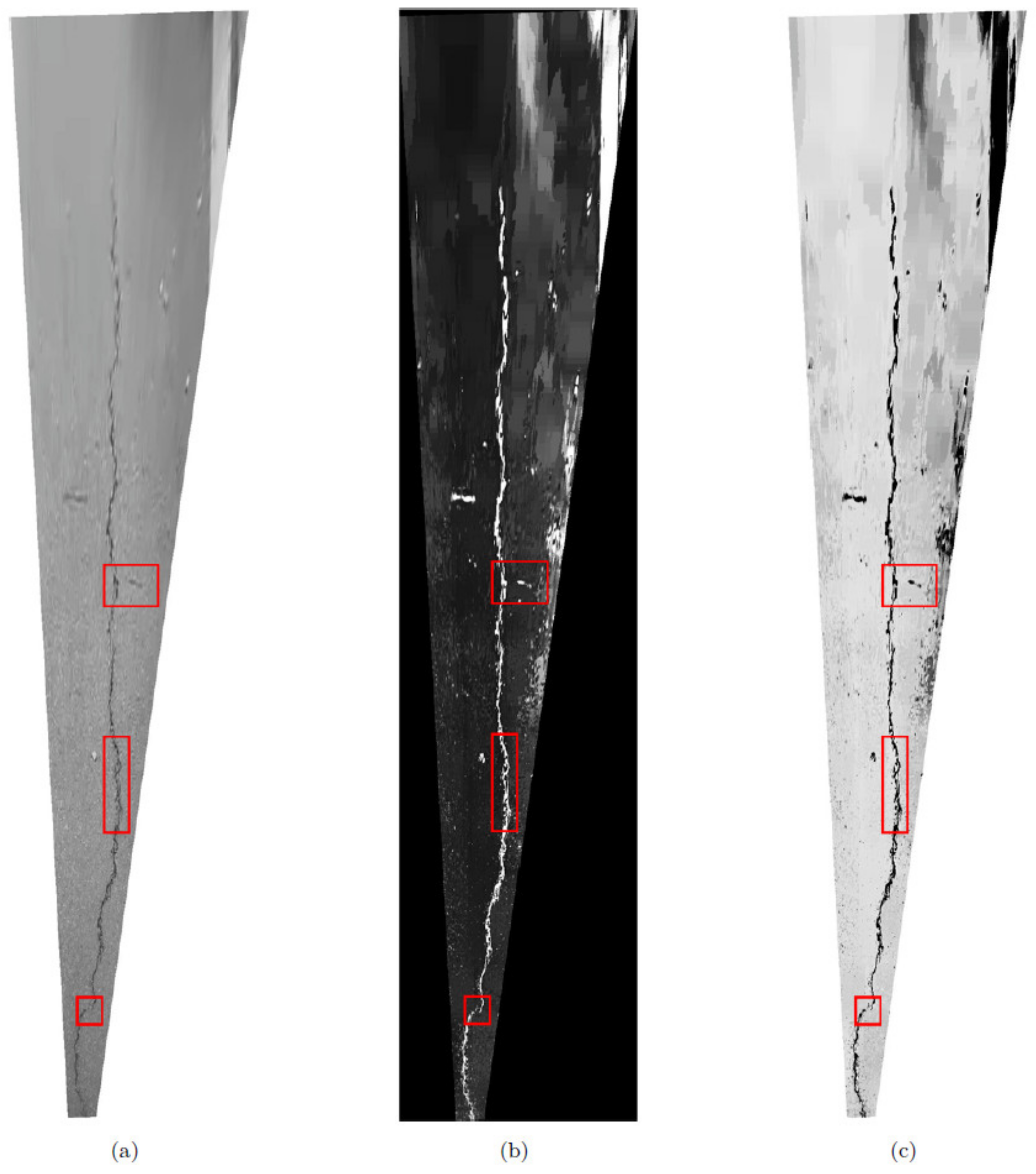
Processing results at different stages. (a) Results after changing IPM. (b) Results after saliency enhancement. (c) Results after flipping saliency images fruit.
Figure 23.
Processing results at different stages. (a) Results after changing IPM. (b) Results after saliency enhancement. (c) Results after flipping saliency images fruit.

Figure 24.
Fracture extraction results. (a) Fracture extraction results. (b) Fracture extraction results superimposed on the original image.
Figure 24.
Fracture extraction results. (a) Fracture extraction results. (b) Fracture extraction results superimposed on the original image.

Figure 25.
Results of fracture extraction. (a) Extraction results without using the proposed method. (b) Extraction results using only F-distance. (c) Only using salient image extraction results.
Figure 25.
Results of fracture extraction. (a) Extraction results without using the proposed method. (b) Extraction results using only F-distance. (c) Only using salient image extraction results.

Figure 26.
Three common shapes of cracks. (a) Transverse crack. (b) Longitudinal crack. (c) Cracked crack.
Figure 26.
Three common shapes of cracks. (a) Transverse crack. (b) Longitudinal crack. (c) Cracked crack.

Figure 27.
Processing results of transverse fractures at each stage. (a) Inverse perspective change map. (b) Salient image. (c) Extracted fractures. (d) Overlay of extracted fractures and original image.
Figure 27.
Processing results of transverse fractures at each stage. (a) Inverse perspective change map. (b) Salient image. (c) Extracted fractures. (d) Overlay of extracted fractures and original image.

Figure 28.
Processing results of longitudinal cracks at different stages. (a) Reverse perspective change diagram. (b) Significance image. (c) Extracted cracks. (d) The superposition result of the extracted cracks and the original image.
Figure 28.
Processing results of longitudinal cracks at different stages. (a) Reverse perspective change diagram. (b) Significance image. (c) Extracted cracks. (d) The superposition result of the extracted cracks and the original image.

Figure 29.
Processing results of alligator crack at different stages. (a) Reverse perspective change diagram. (b) Significance image. (c) Extracted cracks. (d) The superposition result of the extracted cracks and the original image.
Figure 29.
Processing results of alligator crack at different stages. (a) Reverse perspective change diagram. (b) Significance image. (c) Extracted cracks. (d) The superposition result of the extracted cracks and the original image.

Figure 30.
Crack extraction results with lane line interference. (a) Reverse perspective change diagram. (b) Significance image. (c) Extracted cracks. (d) The superposition result of the extracted cracks and the original image.
Figure 30.
Crack extraction results with lane line interference. (a) Reverse perspective change diagram. (b) Significance image. (c) Extracted cracks. (d) The superposition result of the extracted cracks and the original image.

Figure 31.
Comparison of crack extraction accuracy between this method and other methods.

Figure 32.
Examples of false detection by improved YOLOv5 network. (a) The manhole cover was detected as cracked. (b) Example 1 of branches detected as transverse joints. (c) Example 1 of branches detected as Longitudinal Cracks. (d) Example 2 of branches detected as transverse joints.
Figure 32.
Examples of false detection by improved YOLOv5 network. (a) The manhole cover was detected as cracked. (b) Example 1 of branches detected as transverse joints. (c) Example 1 of branches detected as Longitudinal Cracks. (d) Example 2 of branches detected as transverse joints.


Table 1.
Comparison table of crack extraction accuracy between this method and other methods.
| Method | Pr | Re | F1 |
|---|---|---|---|
| Fast-marching method | 0.633 | 0.657 | 0.645 |
| Only using saliency | 0.734 | 0.712 | 0.723 |
| Only using F-distance | 0.722 | 0.786 | 0.753 |
| Ours | 0.893 | 0.871 | 0.882 |
Disclaimer/Publisher’s Note: The statements, opinions and data contained in all publications are solely those of the individual author(s) and contributor(s) and not of MDPI and/or the editor(s). MDPI and/or the editor(s) disclaim responsibility for any injury to people or property resulting from any ideas, methods, instructions or products referred to in the content. |
© 2023 by the authors. Licensee MDPI, Basel, Switzerland. This article is an open access article distributed under the terms and conditions of the Creative Commons Attribution (CC BY) license (https://creativecommons.org/licenses/by/4.0/).
Share and Cite
MDPI and ACS Style
Zhang, S.; Fu, Z.; Li, G.; Liu, A. Lane Crack Detection Based on Saliency. Remote Sens. 2023, 15, 4146. https://doi.org/10.3390/rs15174146
AMA Style
Zhang S, Fu Z, Li G, Liu A. Lane Crack Detection Based on Saliency. Remote Sensing. 2023; 15(17):4146. https://doi.org/10.3390/rs15174146
Chicago/Turabian StyleZhang, Shengyuan, Zhongliang Fu, Gang Li, and Aoxiang Liu. 2023. "Lane Crack Detection Based on Saliency" Remote Sensing 15, no. 17: 4146. https://doi.org/10.3390/rs15174146
Note that from the first issue of 2016, this journal uses article numbers instead of page numbers. See further details here.