
Rapid Landslide Extraction from High-Resolution Remote Sensing Images Using SHAP-OPT-XGBoost
 , ,
, ,  , ,
, ,
Abstract
:
1. Introduction
2. Study Area and Datasets
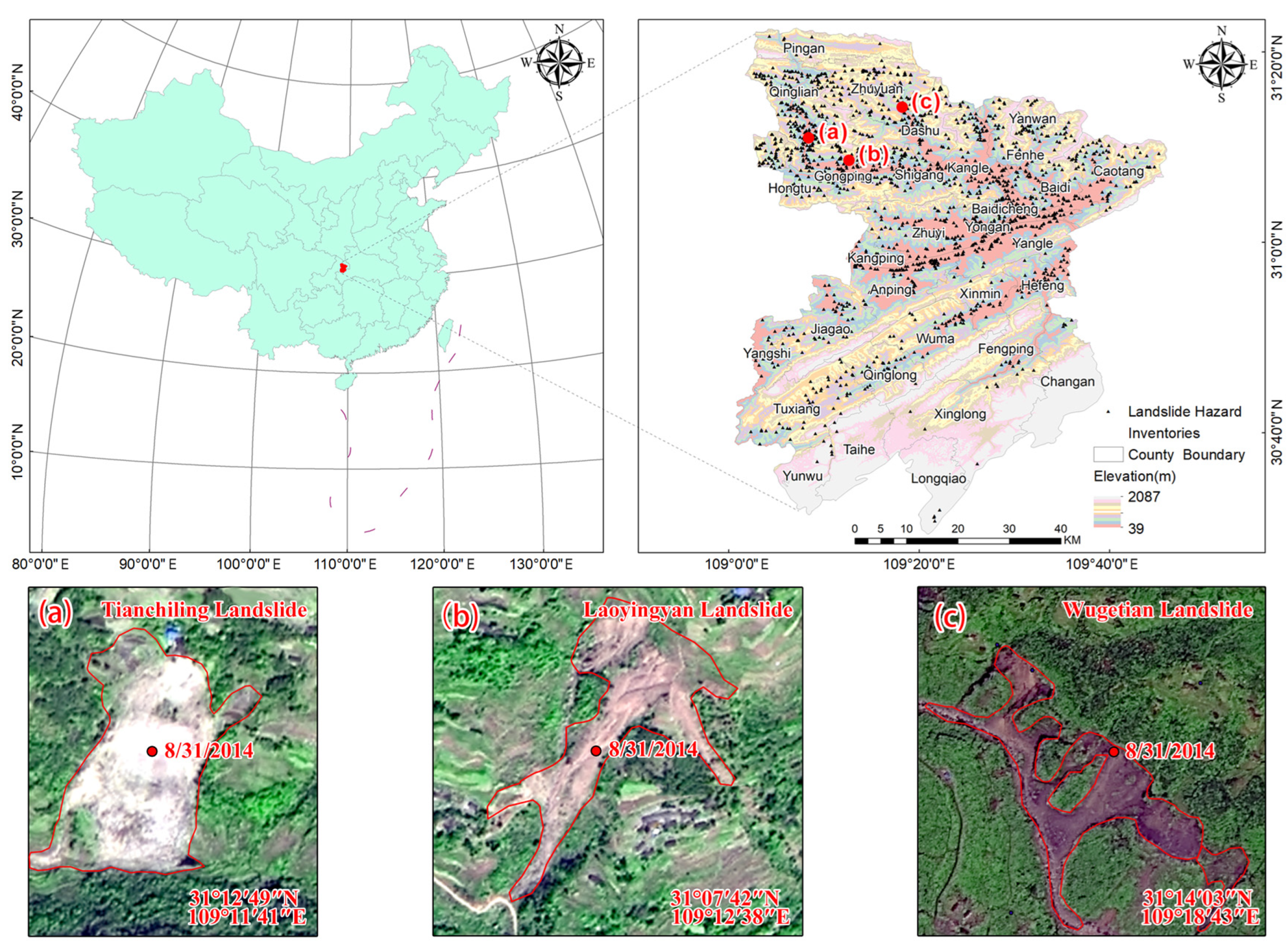
2.1. Study Area
2.2. Data Collection and Preprocessing
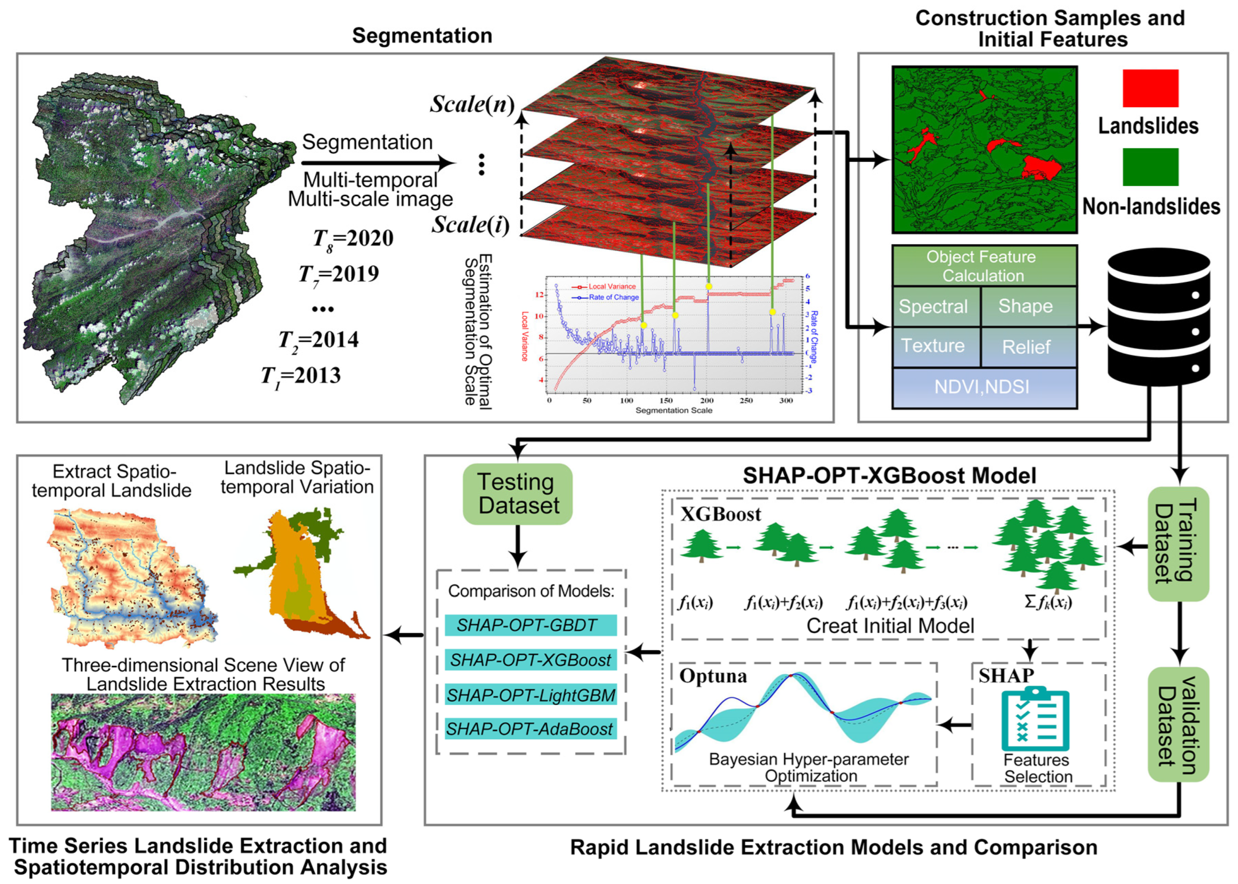
3. Methodology
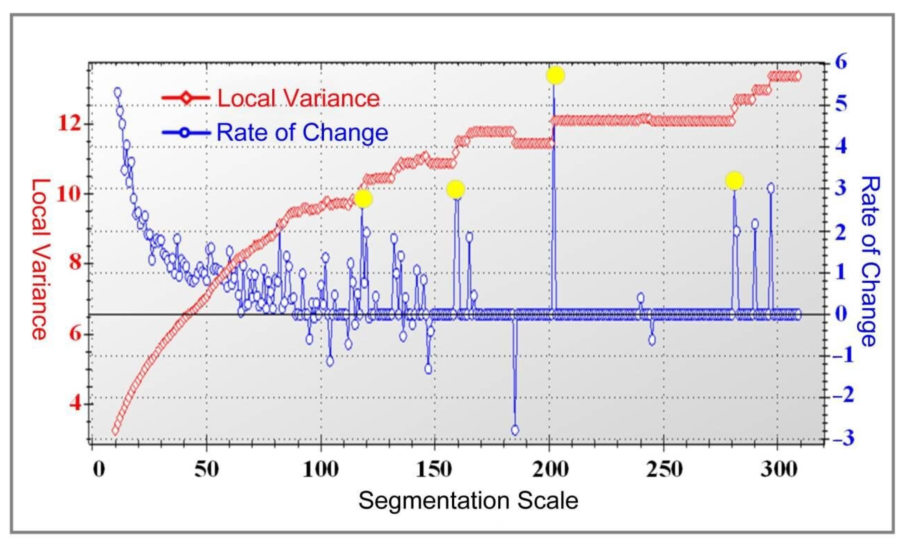
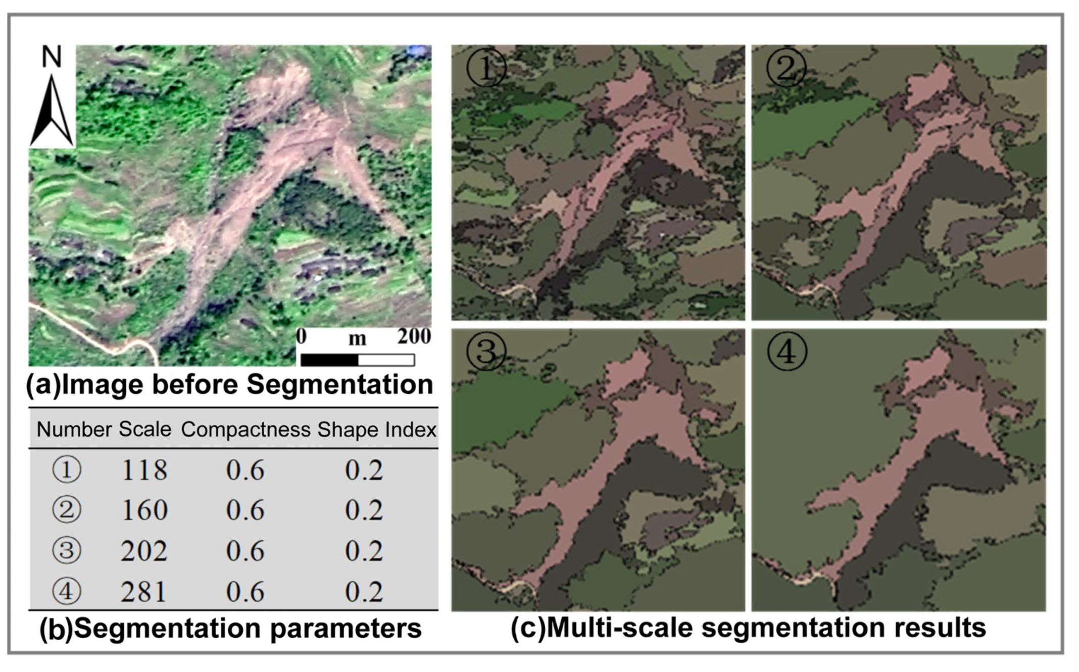
3.1. Image Segmentation
3.2. Construction Samples and Initial Features
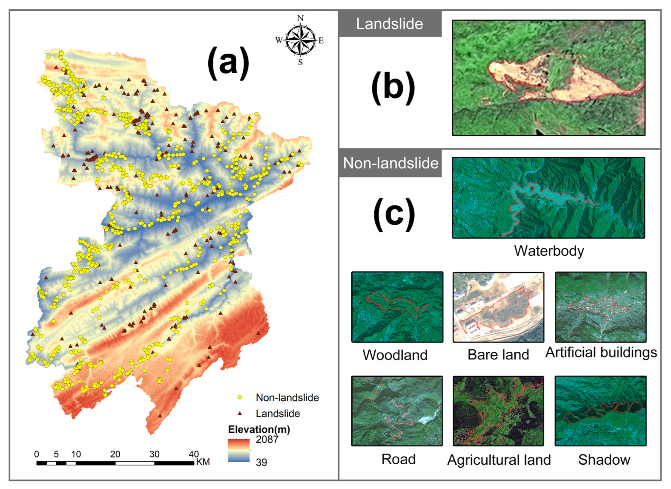
3.2.1. Constructing Samples
3.2.2. Building Initial Feature Set
3.3. Basic Machine Learning Model
3.3.1. GBDT
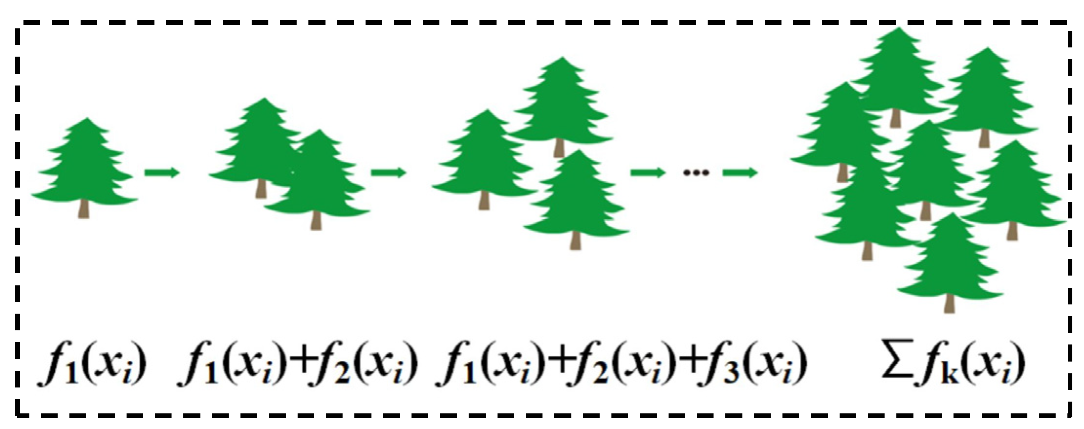
3.3.2. XGBoost
3.3.3. LightGBM
3.3.4. AdaBoost
3.4. Rapid Landslide Extraction Models
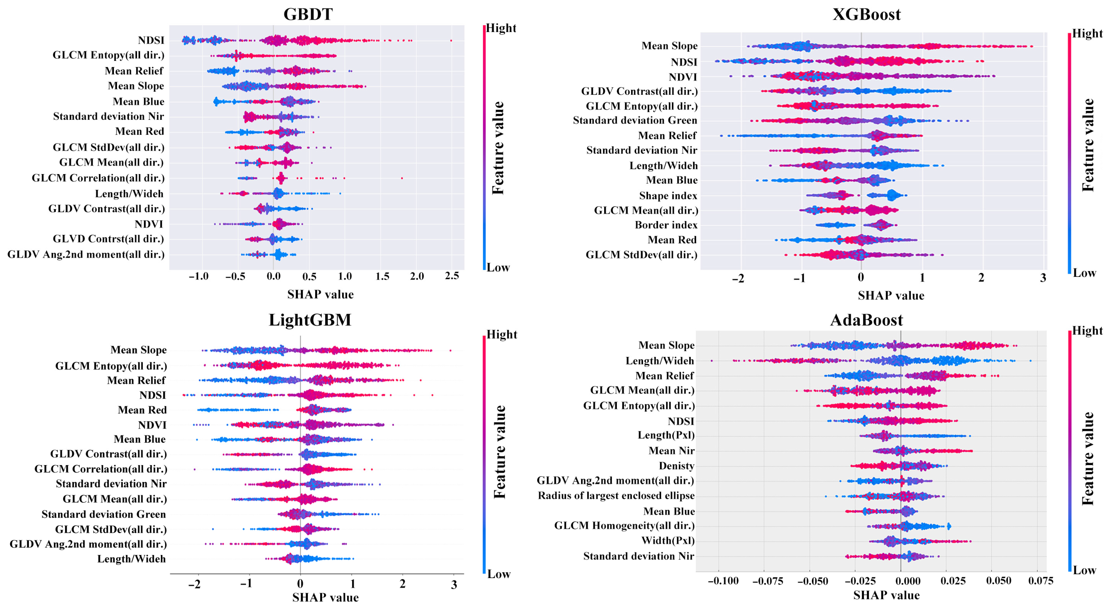
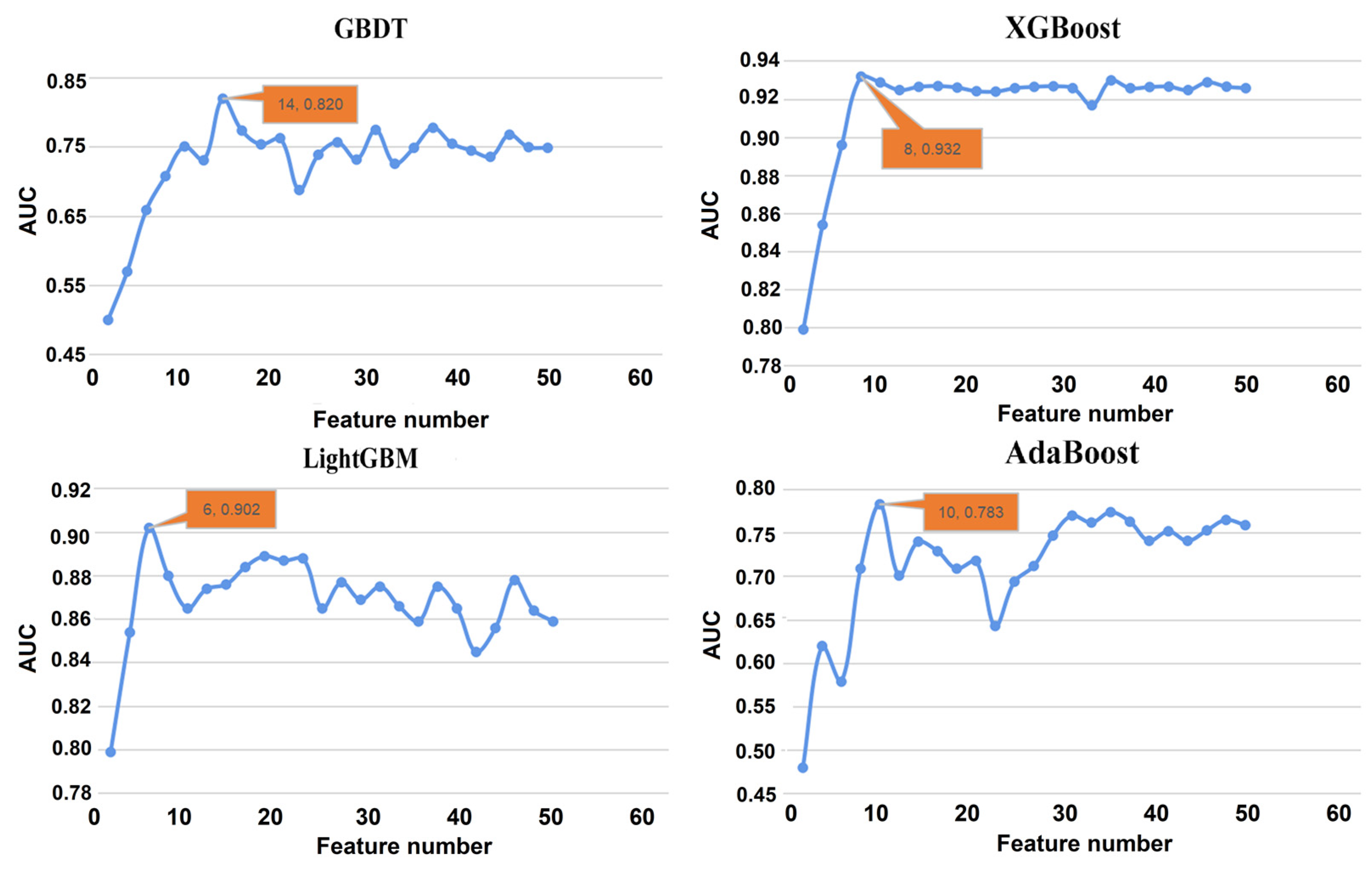
3.4.1. Feature Selection Using SHAP
3.4.2. Optuna Hyperparameter-Tuning
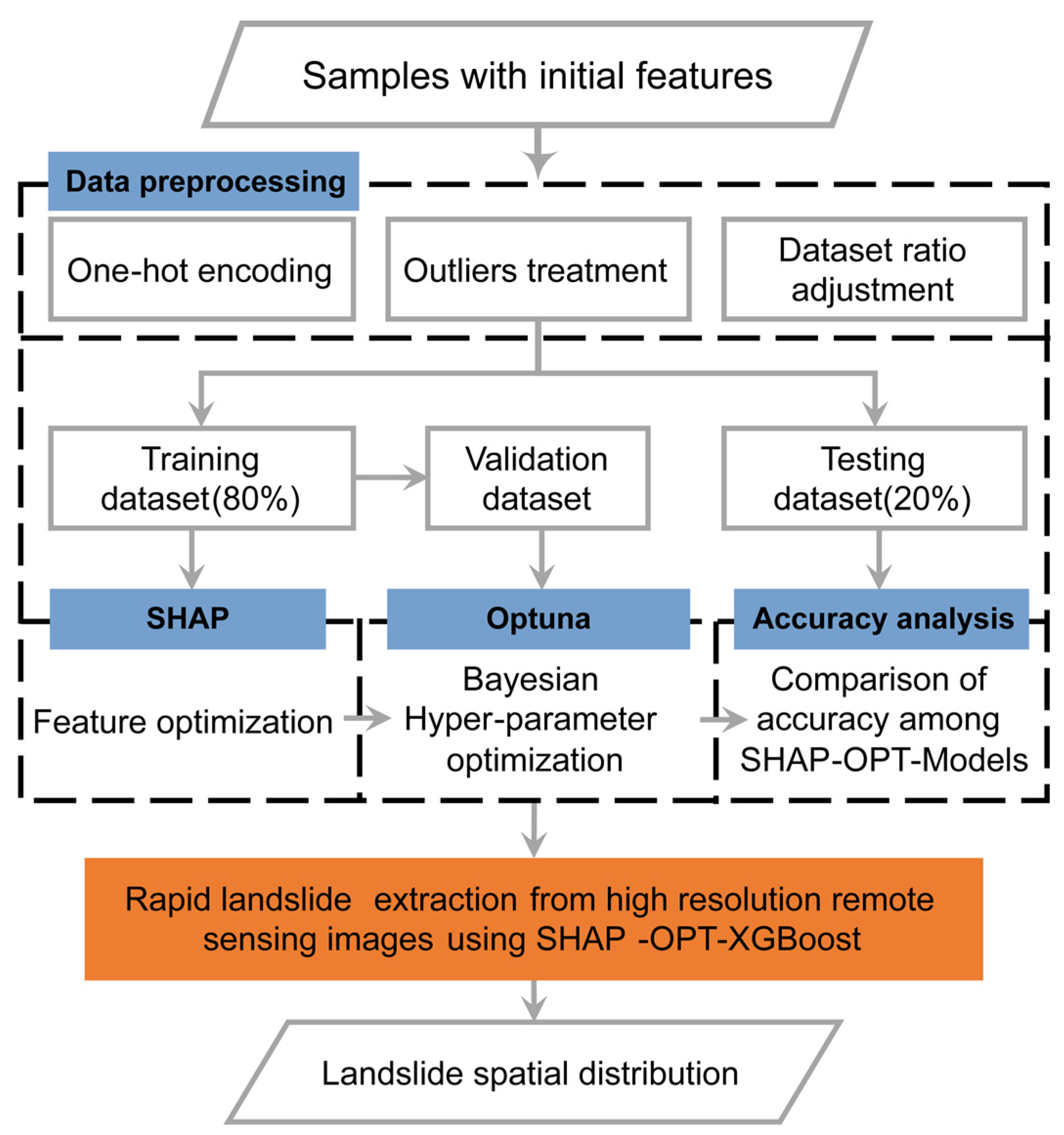
3.4.3. Construction SHAP-OPT-XGBoost Landslide Extraction Model
3.5. Accuracy Evaluation
4. Results
4.1. Preprocessing of High-Resolution Images
4.2. Segmentation
4.3. SHAP Feature Selection
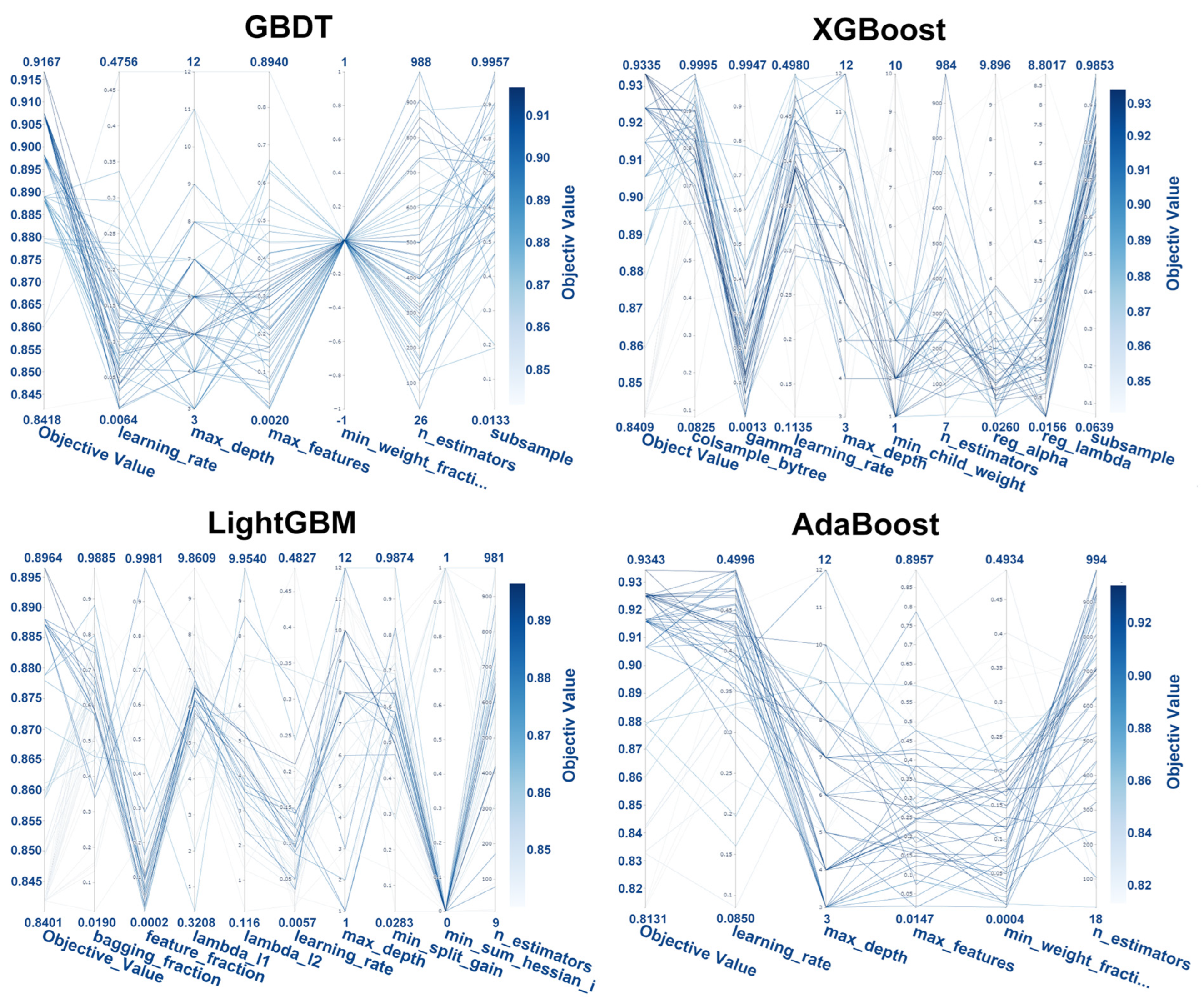
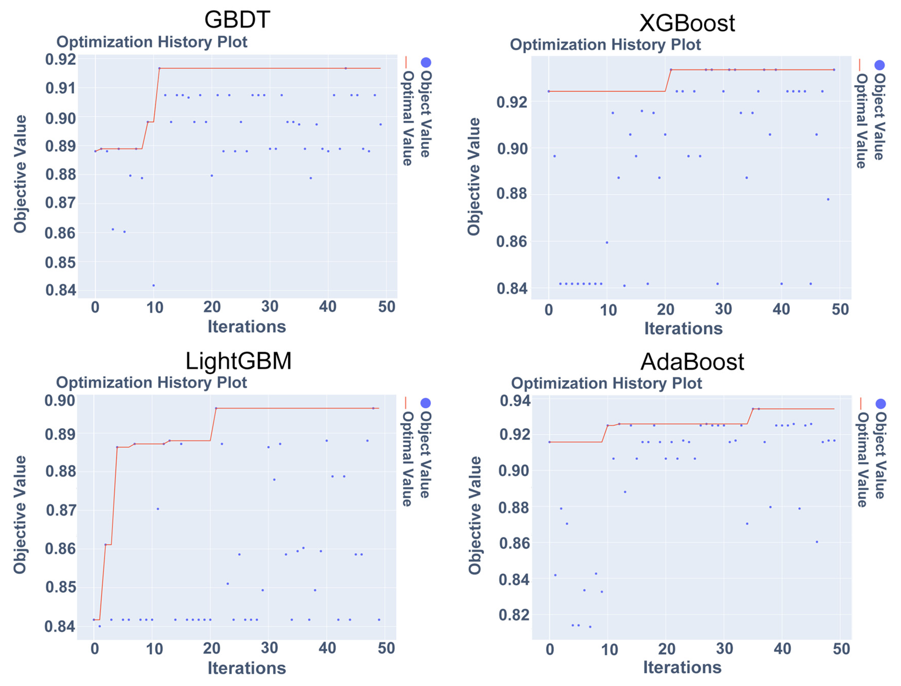
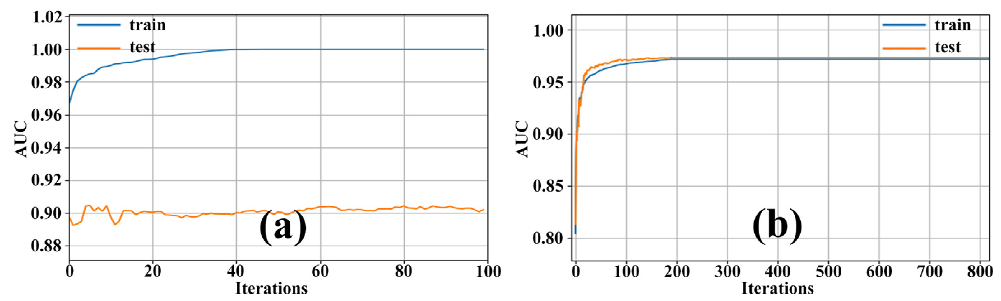
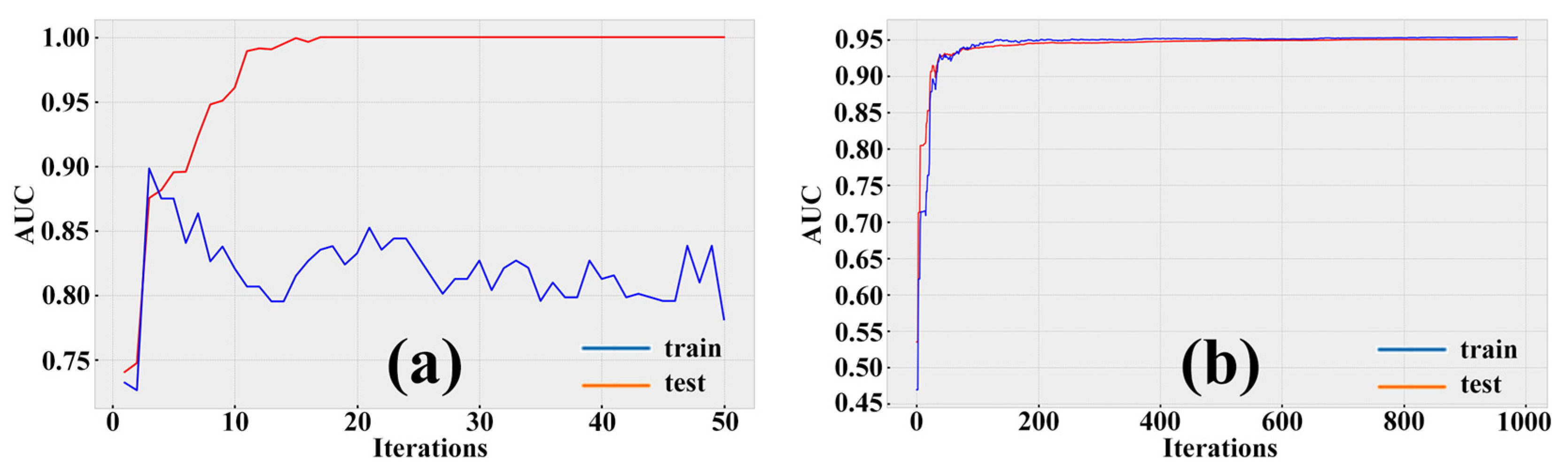
4.4. Optuna Hyperparameter Tuning
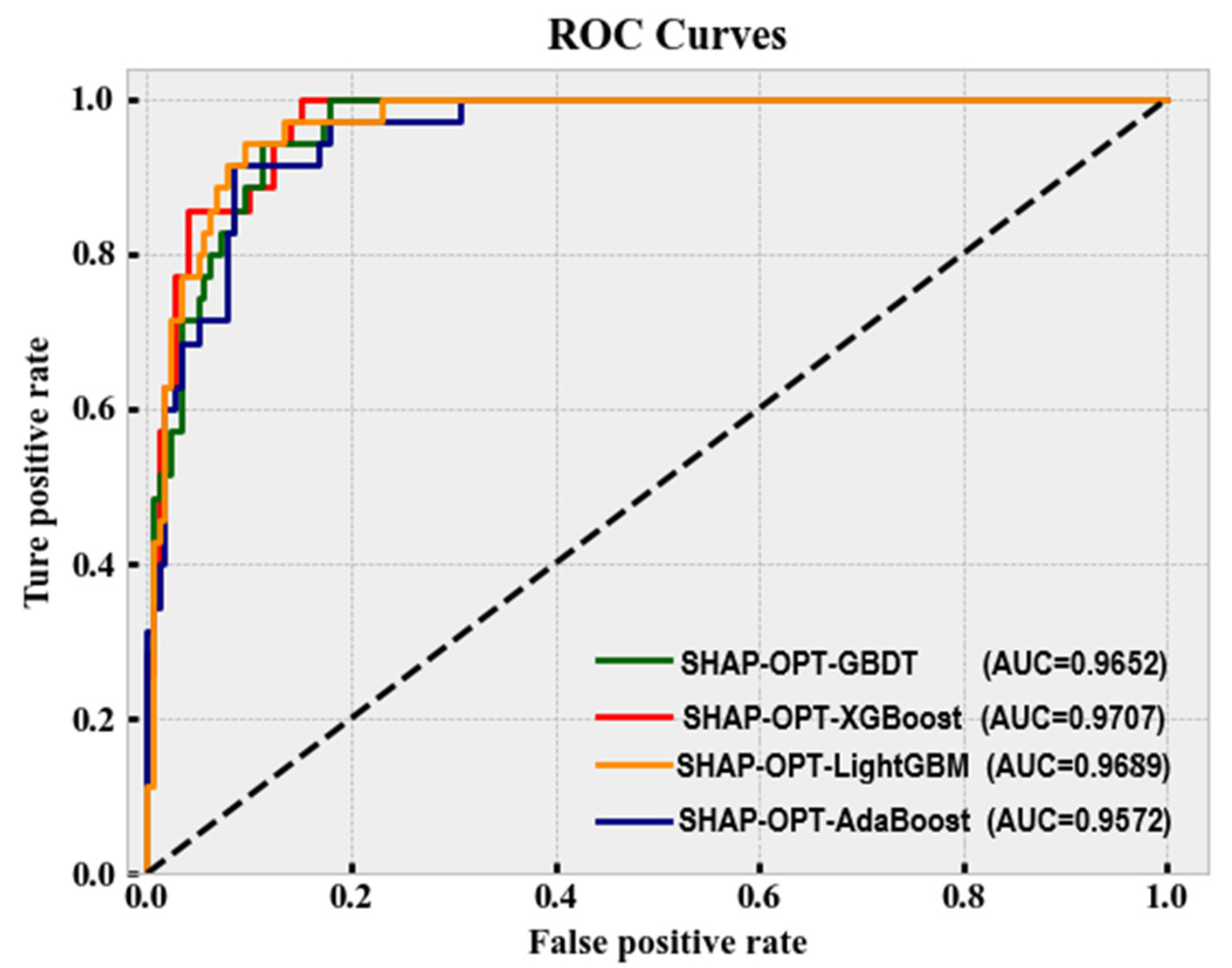
4.5. Comparison of Model Accuracy
4.6. Landslides Information Extraction
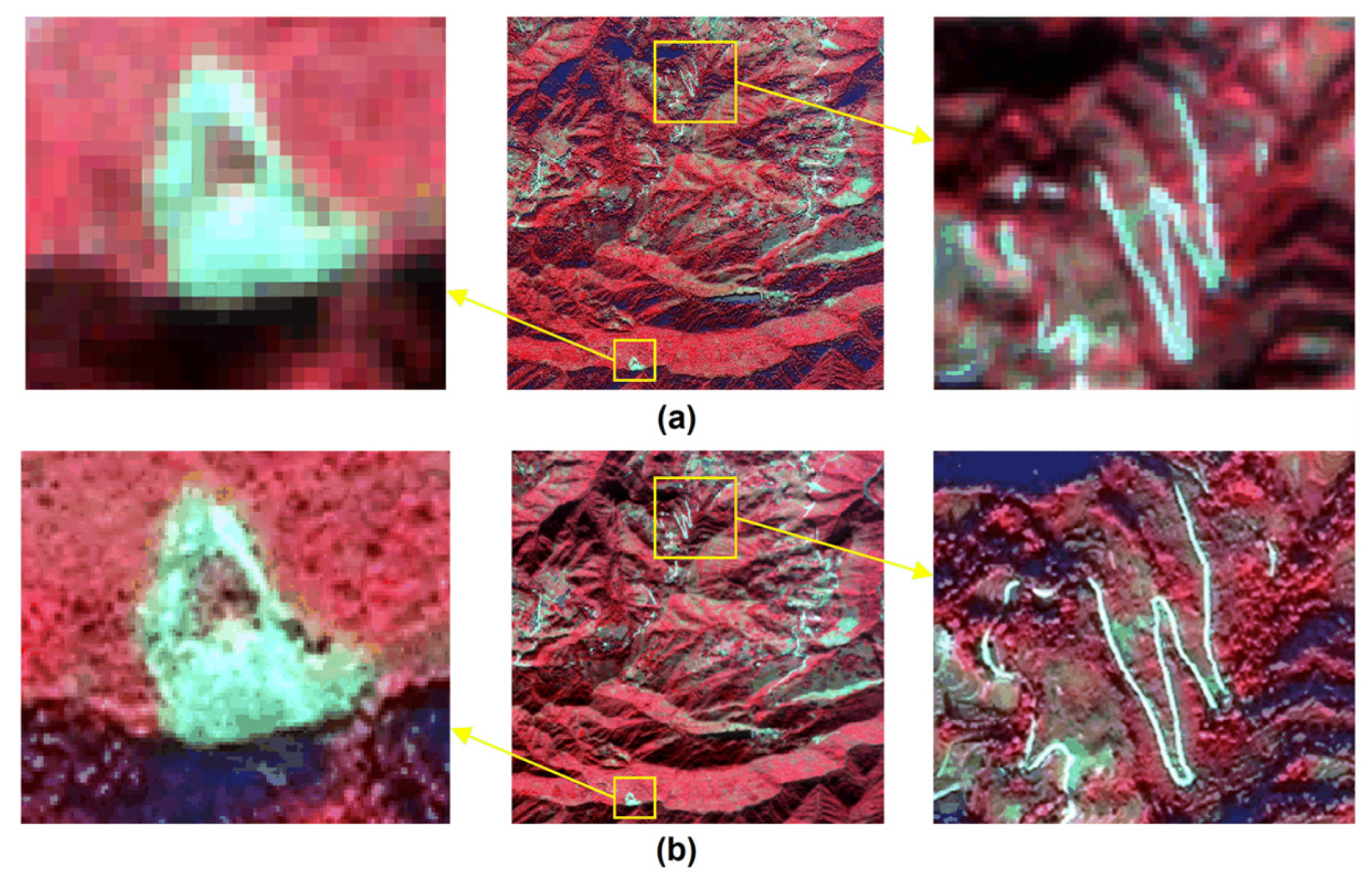
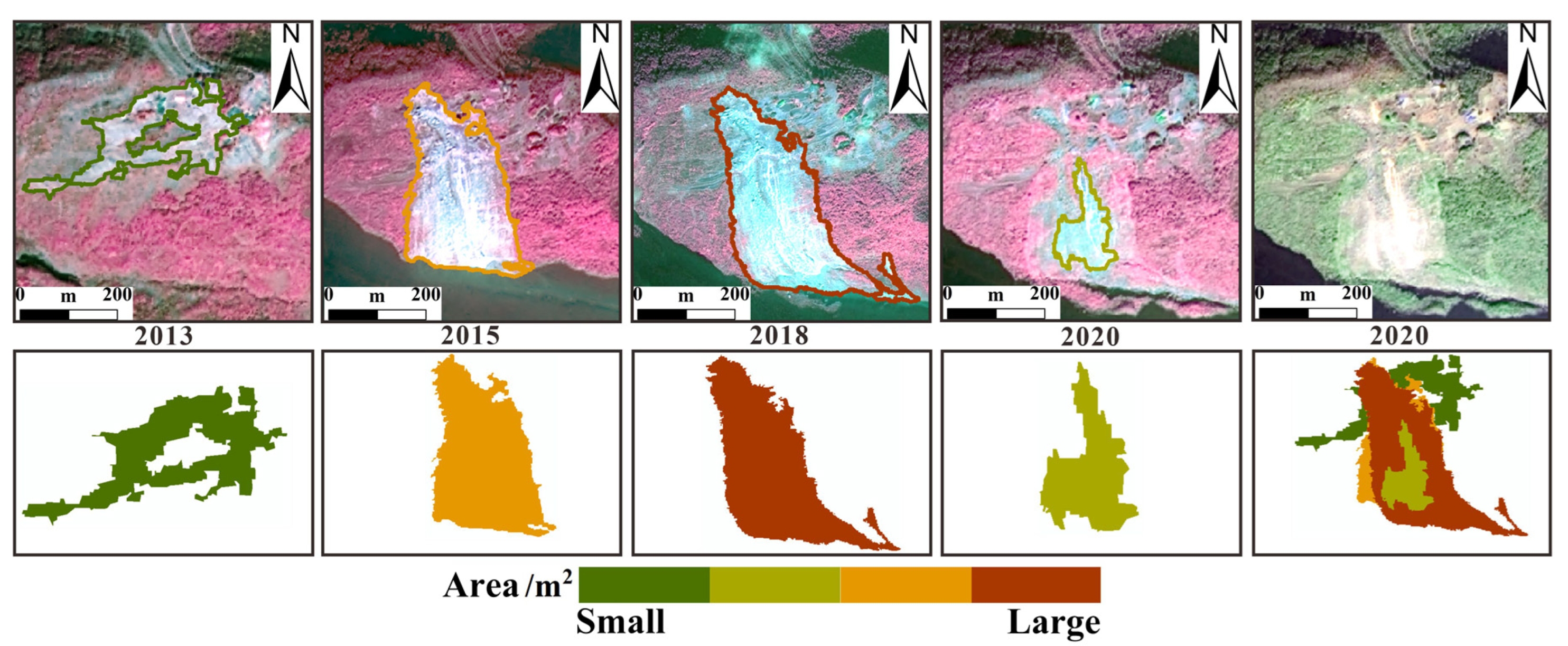
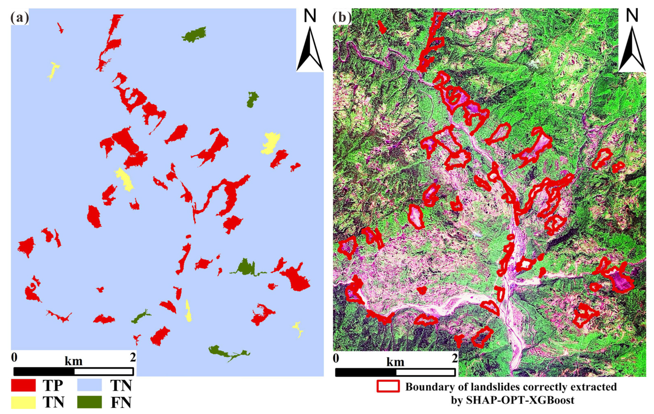
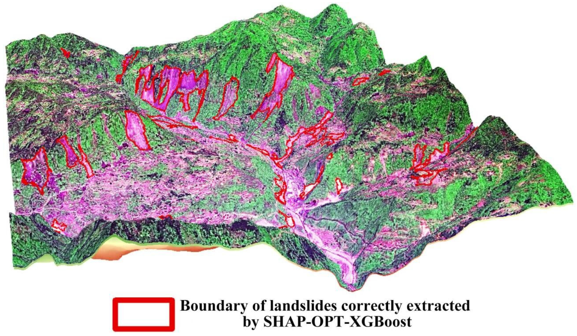
4.6.1. Typical Individual Landslide Analysis
4.6.2. Regional Landslides Analysis
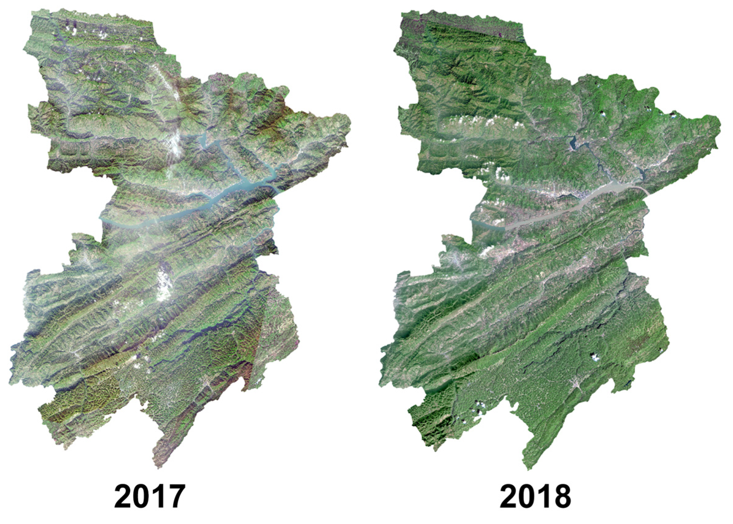
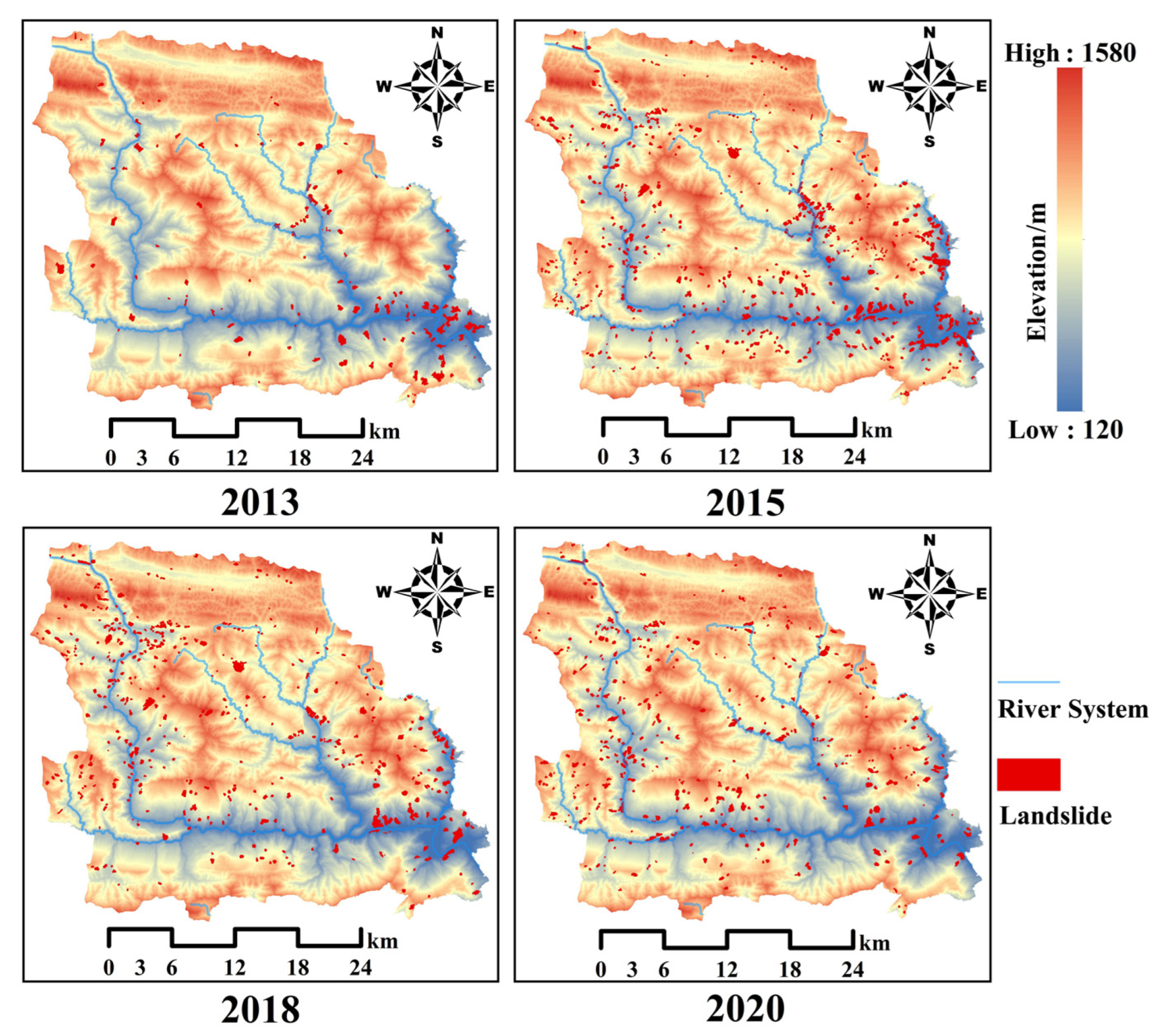
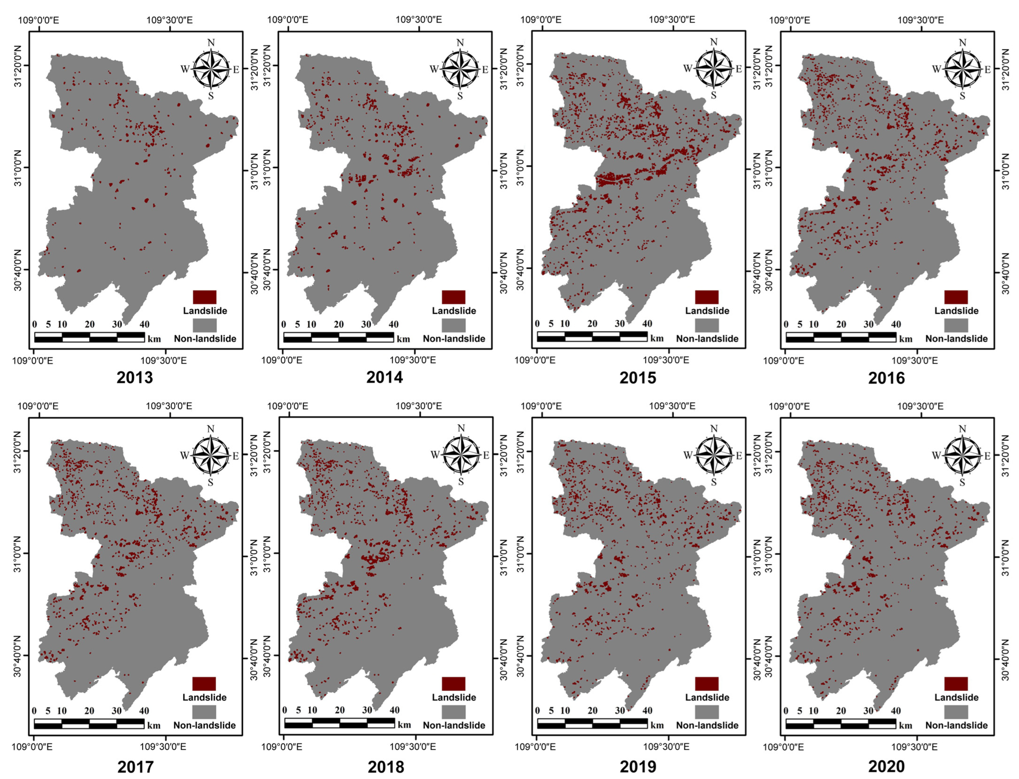
4.6.3. Time-Series Landslides Extraction in Fengjie from 2013 to 2020
5. Discussion
6. Conclusions
Author Contributions
Funding
Data Availability Statement
Acknowledgments
Conflicts of Interest
Appendix A

| Year | Satellite | Sensor | Spatial Resolution/m | Cloud Cover/% | Date of Acquisition | Precipitation Situation | Vegetation Growth Status | |
|---|---|---|---|---|---|---|---|---|
| Panchromatic | Multispectral | |||||||
| 2013 | ZY3-01 | MUX NAD | 2.1 | 5.8 | 2 | 2013/2/10 | less rain | non-growing |
| 2.1 | 5.8 | 9 | 2013/3/26 | less rain | growing | |||
| 2.1 | 5.8 | 1 | 2013/8/11 | rainy | growing | |||
| 2.1 | 5.8 | 9 | 2013/8/11 | rainy | growing | |||
| 2.1 | 5.8 | 0 | 2013/12/2 | less rain | non-growing | |||
| 2.1 | 5.8 | 0 | 2013/12/2 | less rain | non-growing | |||
| 2014 | GF-1 | PMS1 | 2 | 8 | 0 | 2014/3/26 | less rain | growing |
| PMS1 | 2 | 8 | 0 | 2014/3/26 | less rain | growing | ||
| PMS1 | 2 | 8 | 7 | 2014/7/27 | rainy | growing | ||
| PMS1 | 2 | 8 | 2 | 2014/7/27 | rainy | growing | ||
| PMS1 | 2 | 8 | 5 | 2014/7/27 | rainy | growing | ||
| PMS1 | 2 | 8 | 14 | 2014/7/27 | rainy | growing | ||
| PMS2 | 2 | 8 | 2 | 2014/7/27 | rainy | growing | ||
| PMS2 | 2 | 8 | 18 | 2014/7/27 | rainy | growing | ||
| PMS2 | 2 | 8 | 12 | 2014/7/27 | rainy | growing | ||
| PMS1 | 2 | 8 | 5 | 2014/7/31 | rainy | growing | ||
| PMS2 | 2 | 8 | 2 | 2014/7/31 | rainy | growing | ||
| 2015 | GF-1 | PMS2 | 2 | 8 | 4 | 2015/2/17 | less rain | non-growing |
| PMS1 | 2 | 8 | 0 | 2015/3/30 | less rain | growing | ||
| PMS1 | 2 | 8 | 0 | 2015/3/30 | less rain | growing | ||
| PMS2 | 2 | 8 | 0 | 2015/3/30 | less rain | growing | ||
| PMS2 | 2 | 8 | 0 | 2015/3/30 | less rain | growing | ||
| PMS2 | 2 | 8 | 31 | 2015/3/30 | less rain | growing | ||
| PMS1 | 2 | 8 | 1 | 2015/5/14 | rainy | growing | ||
| PMS1 | 2 | 8 | 3 | 2015/5/14 | rainy | growing | ||
| PMS1 | 2 | 8 | 22 | 2015/5/14 | rainy | growing | ||
| PMS1 | 2 | 8 | 9 | 2015/8/16 | rainy | growing | ||
| PMS1 | 2 | 8 | 22 | 2015/8/16 | rainy | growing | ||
| PMS1 | 2 | 8 | 33 | 2015/8/16 | rainy | growing | ||
| 2016 | GF-1 | PMS1 | 2 | 8 | 0 | 2016/8/19 | rainy | growing |
| PMS1 | 2 | 8 | 1 | 2016/8/19 | rainy | growing | ||
| PMS1 | 2 | 8 | 0 | 2016/9/17 | rainy | growing | ||
| PMS1 | 2 | 8 | 2 | 2016/9/17 | rainy | growing | ||
| PMS1 | 2 | 8 | 2 | 2016/9/17 | rainy | growing | ||
| PMS1 | 2 | 8 | 15 | 2016/9/17 | rainy | growing | ||
| PMS2 | 2 | 8 | 0 | 2016/9/17 | rainy | growing | ||
| PMS2 | 2 | 8 | 1 | 2016/9/17 | rainy | growing | ||
| PMS2 | 2 | 8 | 0 | 2016/12/4 | less rain | non-growing | ||
| 2017 | ZY3-01 | MUX NAD | 2.1 | 5.8 | 3 | 2017/10/28 | less rain | non-growing |
| 2.1 | 5.8 | 19 | 2017/10/28 | less rain | non-growing | |||
| GF-1 | PMS1 | 2 | 8 | 1 | 2017/5/13 | rainy | growing | |
| PMS1 | 2 | 8 | 1 | 2017/5/13 | rainy | growing | ||
| PMS2 | 2 | 8 | 0 | 2017/5/13 | rainy | growing | ||
| PMS1 | 2 | 8 | 1 | 2017/11/5 | less rain | non-growing | ||
| PMS2 | 2 | 8 | 0 | 2017/11/5 | less rain | non-growing | ||
| PMS2 | 2 | 8 | 0 | 2017/11/5 | less rain | non-growing | ||
| PMS1 | 2 | 8 | 0 | 2017/11/9 | less rain | non-growing | ||
| PMS2 | 2 | 8 | 0 | 2017/11/9 | less rain | non-growing | ||
| PMS2 | 2 | 8 | 5 | 2017/11/9 | less rain | non-growing | ||
| 2018 | ZY3-01 | MUX NAD | 2.1 | 5.8 | 1 | 2018/8/24 | rainy | growing |
| 2.1 | 5.8 | 2 | 2018/8/24 | rainy | growing | |||
| 2.1 | 5.8 | 0 | 2018/8/29 | rainy | growing | |||
| 2.1 | 5.8 | 0 | 2018/8/29 | rainy | growing | |||
| GF-1 | PMS1 | 2 | 8 | 0 | 2018/1/14 | less rain | non-growing | |
| GF-2 | PMS2 | 2 | 8 | 0 | 2018/1/22 | less rain | non-growing | |
| PMS2 | 2 | 8 | 0 | 2018/1/22 | less rain | non-growing | ||
| 2019 | ZY3-01 | MUX NAD | 2.1 | 5.8 | 0 | 2019/8/13 | rainy | growing |
| 2.1 | 5.8 | 3 | 2019/8/13 | rainy | growing | |||
| 2.1 | 5.8 | 32 | 2019/8/13 | rainy | growing | |||
| GF-6 | PMS | 2 | 8 | 1 | 2019/11/3 | less rain | non-growing | |
| 2 | 8 | 7 | 2019/11/3 | less rain | non-growing | |||
| 2020 | GF-1 | PMS1 | 2 | 8 | 1 | 2020/1/30 | less rain | non-growing |
| PMS1 | 2 | 8 | 1 | 2020/1/30 | less rain | non-growing | ||
| PMS1 | 2 | 8 | 1 | 2020/1/30 | less rain | non-growing | ||
| PMS1 | 2 | 8 | 5 | 2020/1/30 | less rain | non-growing | ||
| PMS2 | 2 | 8 | 3 | 2020/1/30 | less rain | non-growing | ||
| PMS2 | 2 | 8 | 13 | 2020/1/30 | less rain | non-growing | ||
| PMS2 | 2 | 8 | 0 | 2020/11/8 | less rain | non-growing | ||
| PMS2 | 2 | 8 | 0 | 2020/11/8 | less rain | non-growing | ||
| PMS2 | 2 | 8 | 0 | 2020/11/8 | less rain | non-growing | ||
| PMS2 | 2 | 8 | 0 | 2020/11/8 | less rain | non-growing | ||
Appendix B
| Type | Feature | Feature Meaning |
|---|---|---|
| spectrum | Mean I (i = Red, Green, Blue, Nir) | Band means, mean for red, green, blue, near-infrared bands. |
| Standard deviation i (i = Red, Green, Blue, Nir) | Standard deviation of the object in the red, green, blue, and near-infrared bands. | |
| Brightness | Average brightness value of all bands in the image. | |
| Max. diff. | Maximum spectral difference value among all image bands. | |
| Texture | GLCM Homogeneity (all dir.) | Homogeneity of grey-level co-occurrence Matrix (GLCM): Measures the local gray-level uniformity of the image. |
| GLCM Contrast (all dir.) | Contrast of GLCM: Measures the total amount of local variation in the image. | |
| GLCM Dissimilarity (all dir.) | Dissimilarity of GLCM: Similar to contrast, measures the amount of local variation in the image. | |
| GLCM Entropy (all dir.) | Entropy of GLCM: Measures the amount of information in the image. | |
| GLCM Ang. 2nd moment (all dir.) | Second moment of GLCM: Measures the uniformity of the gray-level distribution in the image. | |
| GLCM Mean (all dir.) | Mean of GLCM: Reflects the regularity and uniformity of gray levels in the image. | |
| GLCM StdDev (all dir.) | Standard deviation of GLCM: Reflects the deviation between gray-level values and their mean in the image. | |
| GLCM Correlation (all dir.) | Correlation of GLCM: Reflects the length of extension of certain gray-level values along a certain direction in the image. | |
| GLDV Ang. 2nd moment (all dir.) | Second moment of GLDV: Measures the local homogeneity of the image. | |
| GLDV Entropy (all dir.) | Entropy of GLDV: Measures the complexity of the image. | |
| GLDV Mean(all dir.) | Mean of GLDV: Reflects the regularity and uniformity of gray levels in the image. | |
| GLDV Contrast (all dir.) | Contrast of GLDV: Measures the total amount of local variation in the image. | |
| Geometric | Area (Pxl) | Area: Number of pixels in the object. |
| Border length (Pxl) | Boundary length: Total number of edge pixels in objects shared with other objects. | |
| Length (Pxl) | Length: Product of the total number of pixels in the object and the aspect ratio of length to width. | |
| Length/Width | Aspect ratio: Ratio of length to width of the object. | |
| Volume (Pxl) | Volume: Volume of the object in the image. | |
| Width (Pxl) | Width: Ratio of the total number of pixels in the object and the aspect ratio of length to width. | |
| Asymmetry | Asymmetry: Relative length of the object. | |
| Border index | Boundary index: Indicates the degree of irregularity of the object. | |
| Compactness | Compactness: Describes the compactness of the object. | |
| Radius of smallest enclosing ellipse | Minimum radius of the external ellipse: Describes the similarity between the object’s shape and an ellipse. | |
| Elliptic Fit | Fitting degree of the ellipse: Describes the degree of approximation between the object and a similar-sized ellipse. | |
| Density | Density: Spatial distribution of pixels in the object. | |
| Rectangular Fit | Fitting degree of the rectangle: Degree of approximation between the object and a similar-sized rectangle. | |
| Radius of largest enclosing ellipse | Maximum radius of the internal ellipse: Describes the similarity between the object and an ellipse. | |
| Roundness | Roundness: Degree of similarity between the object and an ellipse. | |
| Shape index | Shape index: Smoothness of the object boundary. | |
| Index | NDVI | Normalized difference vegetation index (NDVI): Calculated as (NIR − R)/(NIR + R), where NIR is the near-infrared band and R is the red band. |
| NDSI | Normalized difference soil index (NDSI): Calculated as (R − G)/(R + G), where R is the red band and G is the green band. | |
| Terrain | Mean i (i = DEM, Slope, Aspect, Relief) | Mean of terrain features: Average value of elevation, slope, aspect, and relief bands in the image object. |
| Standard deviation i (i = DEM, Slope, Aspect, Relief) | Standard deviation of terrain features: Standard deviation of elevation, slope, aspect, and relief bands in the image object. |
References
- Liu, T.; Chen, T.; Niu, R.Q.; Plaza, A. Landslide Detection Mapping Employing CNN, ResNet, and DenseNet in the Three Gorges Reservoir, China. IEEE J Sel Top Appl Earth Obs Remote Sens 2021, 14, 11417–11428. [Google Scholar] [CrossRef]
- Arabameri, A.; Pal, S.C.; Rezaie, F.; Chakrabortty, R.; Chowdhuri, I.; Blaschke, T.; Ngo, P.T.T. Comparison of multi-criteria and artificial intelligence models for land-subsidence susceptibility zonation. J. Environ. Manag. 2021, 284, 18. [Google Scholar] [CrossRef]
- Pang, D.D.; Liu, G.; He, J.; Li, W.L.; Fu, R. Automatic Remote Sensing Identification of Co-Seismic Landslides Using Deep Learning Methods. Forests 2022, 13, 1213. [Google Scholar] [CrossRef]
- Zhao, C.; Lu, Z. Remote Sensing of Landslides—A Review. Remote Sens. 2018, 10, 279. [Google Scholar] [CrossRef] [Green Version]
- Chen, T.H.K.; Prishchepov, A.V.; Fensholt, R.; Sabel, C.E. Detecting and monitoring long-term landslides in urbanized areas with nighttime light data and multi-seasonal Landsat imagery across Taiwan from 1998 to 2017. Remote Sens. Environ. 2019, 225, 317–327. [Google Scholar] [CrossRef]
- Cai, H.J.; Chen, T.; Niu, R.Q.; Plaza, A. Landslide Detection Using Densely Connected Convolutional Networks and Environmental Conditions. IEEE J.-STARS 2021, 14, 5235–5247. [Google Scholar] [CrossRef]
- Yi, Y.N.; Zhang, W.C.; Xu, X.W.; Zhang, Z.J.; Wu, X. Evaluation of neural network models for landslide susceptibility assessment. Int J Digit Earth. 2022, 15, 934–953. [Google Scholar] [CrossRef]
- Liu, Q.; Tang, A.P. Exploring aspects affecting the predicted capacity of landslide susceptibility based on machine learning technology. Geocarto Int. 2022, 37, 14547–14569. [Google Scholar] [CrossRef]
- Wang, S.B.; Zhuang, J.Q.; Zheng, J.; Fan, H.Y.; Kong, J.X.; Zhan, J.W. Application of Bayesian Hyperparameter Optimized Random Forest and XGBoost Model for Landslide Susceptibility Mapping. Front. Earth Sci. 2021, 9, 18. [Google Scholar] [CrossRef]
- Wang, H.J.; Zhang, L.M.; Yin, K.S.; Luo, H.Y.; Li, J.H. Landslide identification using machine learning. Geosci. Front. 2021, 12, 351–364. [Google Scholar] [CrossRef]
- Huang, Y.; Zhao, L. Review on landslide susceptibility mapping using support vector machines. Catena. 2018, 165, 520–529. [Google Scholar] [CrossRef]
- Liu, L.L.; Yang, C.; Wang, X.M. Landslide susceptibility assessment using feature selection-based machine learning models. Geomech. Eng. 2021, 25, 1–16. [Google Scholar]
- Hakim, W.L.; Rezaie, F.; Nur, A.S.; Panahi, M.; Khosravi, K.; Lee, C.W.; Lee, S. Convolutional neural network (CNN) with metaheuristic optimization algorithms for landslide susceptibility mapping in Incheon, South Korea. J. Environ. Manag. 2022, 305, 14. [Google Scholar] [CrossRef]
- Fang, Z.C.; Wang, Y.; Peng, L.; Hong, H.Y. Integration of convolutional neural network and conventional machine learning classifiers for landslide susceptibility mapping. Comput. Geosci. 2020, 139, 15. [Google Scholar] [CrossRef]
- Arabameri, A.; Karimi-Sangchini, E.; Pal, S.C.; Saha, A.; Chowdhuri, I.; Lee, S.; Bui, D.T. Novel Credal Decision Tree-Based Ensemble Approaches for Predicting the Landslide Susceptibility. Remote Sens. 2020, 12, 3389. [Google Scholar] [CrossRef]
- Zhang, S.H.; Wang, Y.W.; Wu, G. Earthquake-Induced Landslide Susceptibility Assessment Using a Novel Model Based on Gradient Boosting Machine Learning and Class Balancing Methods. Remote Sens. 2022, 14, 5945. [Google Scholar] [CrossRef]
- Jia, D.; Yang, L.; Gao, X.; Li, K. Assessment of a New Solar Radiation Nowcasting Method Based on FY-4A Satellite Imagery, the McClear Model and SHapley Additive exPlanations (SHAP). Remote Sens. 2023, 15, 2245. [Google Scholar] [CrossRef]
- Zhou, Y.; Wu, W.; Liu, H. Exploring the Influencing Factors in Identifying Soil Texture Classes Using Multitemporal Landsat-8 and Sentinel-2 Data. Remote Sens. 2022, 14, 5571. [Google Scholar] [CrossRef]
- Akiba, T.; Sano, S.; Yanase, T.; Ohta, T.; Koyama, M.; Assoc Comp, M. Optuna: A Next-generation Hyperparameter Optimization Framework. ACM 2019, 8, 2623–2631. [Google Scholar]
- Bai, S.B.; Wang, J.; Lu, G.N.; Zhou, P.G.; Hou, S.S.; Xu, S.N. GIS-based logistic regression for landslide susceptibility mapping of the Zhongxian segment in the Three Gorges area, China. Geomorphology 2010, 115, 23–31. [Google Scholar] [CrossRef]
- Shafiq, M.; Gu, Z. Deep Residual Learning for Image Recognition: A Survey. Appl. Sci. 2022, 12, 8972. [Google Scholar] [CrossRef]
- Gu, H.; Han, Y.; Yang, Y.; Li, H.; Liu, Z.; Soergel, U.; Blaschke, T.; Cui, S. An Efficient Parallel Multi-Scale Segmentation Method for Remote Sensing Imagery. Remote Sens. 2018, 10, 590. [Google Scholar] [CrossRef] [Green Version]
- Su, T.F. Efficient paddy field mapping using Landsat-8 imagery and object-based image analysis based on advanced fractal net evolution approach. GISci. Remote Sens. 2017, 54, 354–380. [Google Scholar] [CrossRef]
- Zeng, Y.L.; Li, J.; Liu, Q.H.; Li, L.H.; Xu, B.D.; Yin, G.F.; Peng, J.J. A Sampling Strategy for Remotely Sensed LAI Product Validation Over Heterogeneous Land Surfaces. IEEE J.-STARS 2014, 7, 3128–3142. [Google Scholar] [CrossRef]
- Lin, W.; Li, Y. Parallel Regional Segmentation Method of High-Resolution Remote Sensing Image Based on Minimum Spanning Tree. Remote Sens. 2020, 12, 783. [Google Scholar] [CrossRef] [Green Version]
- Sun, Z.; Wang, Y.F.; Pan, L.; Xie, Y.H.; Zhang, B.; Liang, R.T.; Sun, Y.J. Pine wilt disease detection in high-resolution UAV images using object-oriented classification. J. For. Res. 2022, 33, 1377–1389. [Google Scholar] [CrossRef]
- Dragut, L.; Tiede, D.; Levick, S.R. ESP: A tool to estimate scale parameter for multiresolution image segmentation of remotely sensed data. Int. J. Geogr. Inf. Sci. 2010, 24, 859–871. [Google Scholar] [CrossRef] [Green Version]
- Dragut, L.; Belgiu, M.; Popescu, G.; Bandura, P. Sensitivity of multiresolution segmentation to spatial extent. Int. J. Appl. Earth Obs. Geoinf. 2019, 81, 146–153. [Google Scholar]
- Yang, R.; Zhang, F.; Xia, J.; Wu, C. Landslide Extraction Using Mask R-CNN with Background-Enhancement Method. Remote Sens. 2022, 14, 2206. [Google Scholar] [CrossRef]
- Chen, C.Y.; Chang, J.M. Landslide dam formation susceptibility analysis based on geomorphic features. Landslides 2016, 13, 1019–1033. [Google Scholar] [CrossRef]
- Yu, B.; Xu, C.; Chen, F.; Wang, N.; Wang, L. HADeenNet: A hierarchical-attention multi-scale deconvolution network for landslide detection. Int. J. Appl. Earth Obs. Geoinf. 2022, 111, 12. [Google Scholar] [CrossRef]
- Sun, D.L.; Wu, X.Q.; Wen, H.J.; Gu, Q.Y. A LightGBM-based landslide susceptibility model considering the uncertainty of non-landslide samples. Geomat. Nat. Hazards Risk 2023, 14, 31. [Google Scholar] [CrossRef]
- Liu, R.; Peng, J.; Leng, Y.; Lee, S.; Panahi, M.; Chen, W.; Zhao, X. Hybrids of Support Vector Regression with Grey Wolf Optimizer and Firefly Algorithm for Spatial Prediction of Landslide Susceptibility. Remote Sens. 2021, 13, 4966. [Google Scholar] [CrossRef]
- Rosi, A.; Tofani, V.; Tanteri, L.; Stefanelli, C.T.; Agostini, A.; Catani, F.; Casagli, N. The new landslide inventory of Tuscany (Italy) updated with PS-InSAR: Geomorphological features and landslide distribution. Landslides 2018, 15, 5–19. [Google Scholar] [CrossRef] [Green Version]
- Friedman, J.H. Greedy function approximation: A gradient boosting machine. Ann. Stat. 2001, 29, 1189–1232. [Google Scholar] [CrossRef]
- Rong, G.; Alu, S.; Li, K.; Su, Y.; Zhang, J.; Zhang, Y.; Li, T. Rainfall Induced Landslide Susceptibility Mapping Based on Bayesian Optimized Random Forest and Gradient Boosting Decision Tree Models—A Case Study of Shuicheng County, China. Water 2020, 12, 3066. [Google Scholar] [CrossRef]
- Chen, T.; Guestrin, C. XGBoost: A Scalable Tree Boosting System. In Proceedings of the 22nd ACM SIGKDD International Conference on Knowledge Discovery and Data Mining, San Francisco, CA, USA, 13–17 August 2016. [Google Scholar]
- Shi, N.; Li, Y.L.; Wen, L.F.; Zhang, Y. Rapid prediction of landslide dam stability considering the missing data using XGBoost algorithm. Landslides 2022, 19, 2951–2963. [Google Scholar] [CrossRef]
- Kavzoglu, T.; Teke, A. Predictive Performances of Ensemble Machine Learning Algorithms in Landslide Susceptibility Mapping Using Random Forest, Extreme Gradient Boosting (XGBoost) and Natural Gradient Boosting (NGBoost). Arab. J. Sci. Eng. 2022, 47, 7367–7385. [Google Scholar] [CrossRef]
- Pham, Q.B.; Achour, Y.; Ali, S.A.; Parvin, F.; Vojtek, M.; Vojtekova, J.; Al-Ansari, N.; Achu, A.L.; Costache, R.; Khedher, K.M.; et al. A comparison among fuzzy multi-criteria decision making, bivariate, multivariate and machine learning models in landslide susceptibility mapping. Geomat. Nat. Hazards Risk 2021, 12, 1741–1777. [Google Scholar] [CrossRef]
- Ke, G.; Meng, Q.; Finley, T.; Wang, T.; Chen, W.; Ma, W.; Liu, T.Y. LightGBM: A highly efficient gradient boosting decision tree. Adv. Neural Inf. Process. Syst. 2017, 30, 3149–3157. [Google Scholar]
- Liu, R.; Ding, Y.K.; Sun, D.L.; Wen, H.J.; Gu, Q.Y.; Shi, S.X.; Liao, M.Y. Insights into spatial differential characteristics of landslide susceptibility from sub-region to whole-region cased by northeast Chongqing, China. Geomat. Nat. Hazards Risk 2023, 14, 25. [Google Scholar] [CrossRef]
- Bentejac, C.; Csorgo, A.; Martinez-Munoz, G. A comparative analysis of gradient boosting algorithms. Artif. Intell. Rev. 2021, 54, 1937–1967. [Google Scholar] [CrossRef]
- Liang, W.; Luo, S.; Zhao, G.; Wu, H. Predicting Hard Rock Pillar Stability Using GBDT, XGBoost, and LightGBM Algorithms. Mathematics 2020, 8, 765. [Google Scholar] [CrossRef]
- Freund, Y.; Schapire, R. A decision-theoretic generalization of online learning and an application to boosting. JCSS 1997, 55, 119–139. [Google Scholar]
- Wu, Y.L.; Ke, Y.T.; Chen, Z.; Liang, S.Y.; Zhao, H.L.; Hong, H.Y. Application of alternating decision tree with AdaBoost and bagging ensembles for landslide susceptibility mapping. Catena 2020, 187, 17. [Google Scholar] [CrossRef]
- Nhu, V.-H.; Mohammadi, A.; Shahabi, H.; Ahmad, B.B.; Al-Ansari, N.; Shirzadi, A.; Clague, J.J.; Jaafari, A.; Chen, W.; Nguyen, H. Landslide Susceptibility Mapping Using Machine Learning Algorithms and Remote Sensing Data in a Tropical Environment. Int. J. Environ. Res. Public Health 2020, 17, 4933. [Google Scholar] [CrossRef]
- Jiang, Z.; Wang, M.; Liu, K. Comparisons of Convolutional Neural Network and Other Machine Learning Methods in Landslide Susceptibility Assessment: A Case Study in Pingwu. Remote Sens. 2023, 15, 798. [Google Scholar] [CrossRef]
- Naghibi, S.A.; Moghaddam, D.D.; Kalantar, B.; Pradhan, B.; Kisi, O. A comparative assessment of GIS-based data mining models and a novel ensemble model in groundwater well potential mapping. J. Hydrol. 2017, 548, 471–483. [Google Scholar] [CrossRef]
- Lundberg, S.; Lee, S.I. A Unified Approach to Interpreting Model Predictions. Adv. Neural Inf. Process. Syst. 2017, 30, 4768–4777. [Google Scholar]
- Ekmekcioglu, O.; Koc, K. Explainable step-wise binary classification for the susceptibility assessment of geo-hydrological hazards. Catena 2022, 216, 18. [Google Scholar] [CrossRef]
- Zhang, J.Y.; Ma, X.L.; Zhang, J.L.; Sun, D.L.; Zhou, X.Z.; Mi, C.L.; Wen, H.J. Insights into geospatial heterogeneity of landslide susceptibility based on the SHAP-XGBoost model. J. Environ. Manag. 2023, 332, 20. [Google Scholar] [CrossRef] [PubMed]
- Kavzoglu, T.; Teke, A. Advanced hyperparameter optimization for improved spatial prediction of shallow landslides using extreme gradient boosting (XGBoost). Bull. Eng. Geol. Environ. 2022, 81, 22. [Google Scholar] [CrossRef]
- Pradhan, B.; Sameen, M.I.; Al-Najjar, H.A.H.; Sheng, D.; Alamri, A.M.; Park, H.-J. A Meta-Learning Approach of Optimisation for Spatial Prediction of Landslides. Remote Sens. 2021, 13, 4521. [Google Scholar] [CrossRef]
- Ma, J.W.; Xia, D.; Guo, H.X.; Wang, Y.K.; Niu, X.X.; Liu, Z.Y.; Jiang, S. Metaheuristic-based support vector regression for landslide displacement prediction: A comparative study. Landslides 2022, 19, 2489–2511. [Google Scholar] [CrossRef]
- Sestras, P.; Bilaco, T.; Rosca, S.; Nas, S.; Bondrea, M.V.; Galgau, R.; Veres, I.; Salagean, T.; Spalevic, V.; Cîmpeanu, S.M. Landslides Susceptibility Assessment Based on GIS Statistical Bivariate Analysis in the Hills Surrounding a Metropolitan Area. Sustainability 2019, 11, 1362. [Google Scholar] [CrossRef] [Green Version]
- Hussain, M.A.; Chen, Z.; Zheng, Y.; Shoaib, M.; Shah, S.U.; Ali, N.; Afzal, Z. Landslide Susceptibility Mapping Using Machine Learning Algorithm Validated by Persistent Scatterer In-SAR Technique. Sensors 2022, 22, 3119. [Google Scholar] [CrossRef]
- Zhang, Y.; Ge, T.; Tian, W.; Liou, Y.-A. Debris Flow Susceptibility Mapping Using Machine-Learning Techniques in Shigatse Area, China. Remote Sens. 2019, 11, 2801. [Google Scholar] [CrossRef] [Green Version]
- Riaz, M.T.; Basharat, M.; Brunetti, M.T. Assessing the effectiveness of alternative landslide partitioning in machine learning methods for landslide prediction in the complex Himalayan terrain. Prog Phys Geog. 2023, 47, 315–347. [Google Scholar] [CrossRef]
- Lu, H.; Ma, L.; Fu, X.; Liu, C.; Li, N. Landslides Information Extraction Using Object-Oriented Image Analysis Paradigm Based on Deep Learning and Transfer Learning. Remote Sens. 2020, 12, 752. [Google Scholar] [CrossRef] [Green Version]


| Prediction Situation | Actual Situation | |
|---|---|---|
| Landslide | Non-Landslide | |
| Landslide | True positive (TP) | False positive (FP) |
| Non-landslide | False negative (FN) | True negative TN |
| Hyperparameter | Defaults | Optimal Value | Parameter Meaning |
|---|---|---|---|
| learning_rate | 0.3 | 0.25 | learning rate |
| max_depth | 6 | 10 | the maximum depth of the tree |
| n_estimators | 500 | 700 | Number of estimators |
| min_child_weight | 1 | 2 | Min leaf weight |
| subsample | 1 | 0.4 | Subsample of training instances |
| colsample_bytree | 1 | 0.5 | Feature subsampling |
| reg_alpha | 0 | 7 | L1 regularization of weights |
| reg_lambda | 1 | 4 | L2 regularization of weights |
| gamma | 0 | 0.3 | Minimum loss reduction |
| Algorithm | Accuracy/% | Precision/% | Recall/% | Kappa | Training Time/s |
|---|---|---|---|---|---|
| SHAP-OPT-XGBoost | 96.26 | 90.91 | 85.71 | 0.8602 | 1.16 |
| SHAP-OPT-GBDT | 93.93 | 82.35 | 80.00 | 0.7754 | 1.28 |
| SHAP-OPT-LightGBM | 95.79 | 86.11 | 88.57 | 0.8480 | 1.06 |
| SHAP-OPT-AdaBoost | 92.99 | 83.33 | 71.43 | 0.7282 | 0.97 |
| Year | Accuracy/% | Misclassification Rate/% | Omission Rate/% |
|---|---|---|---|
| 2013 | 74.31 | 25.69 | 16.92 |
| 2015 | 86.76 | 13.24 | 8.34 |
| 2018 | 89.77 | 10.23 | 18.56 |
| 2020 | 82.14 | 17.86 | 11.33 |
| Year | 2013 | 2014 | 2015 | 2016 | 2017 | 2018 | 2019 | 2020 |
|---|---|---|---|---|---|---|---|---|
| landslide area (km2) | 19.26 | 32.92 | 55.42 | 42.74 | 39.65 | 45.76 | 35.02 | 39.35 |
Disclaimer/Publisher’s Note: The statements, opinions and data contained in all publications are solely those of the individual author(s) and contributor(s) and not of MDPI and/or the editor(s). MDPI and/or the editor(s) disclaim responsibility for any injury to people or property resulting from any ideas, methods, instructions or products referred to in the content. |
© 2023 by the authors. Licensee MDPI, Basel, Switzerland. This article is an open access article distributed under the terms and conditions of the Creative Commons Attribution (CC BY) license (https://creativecommons.org/licenses/by/4.0/).
Share and Cite
Lin, N.; Zhang, D.; Feng, S.; Ding, K.; Tan, L.; Wang, B.; Chen, T.; Li, W.; Dai, X.; Pan, J.; et al. Rapid Landslide Extraction from High-Resolution Remote Sensing Images Using SHAP-OPT-XGBoost. Remote Sens. 2023, 15, 3901. https://doi.org/10.3390/rs15153901
Lin N, Zhang D, Feng S, Ding K, Tan L, Wang B, Chen T, Li W, Dai X, Pan J, et al. Rapid Landslide Extraction from High-Resolution Remote Sensing Images Using SHAP-OPT-XGBoost. Remote Sensing. 2023; 15(15):3901. https://doi.org/10.3390/rs15153901
Chicago/Turabian StyleLin, Na, Di Zhang, Shanshan Feng, Kai Ding, Libing Tan, Bin Wang, Tao Chen, Weile Li, Xiaoai Dai, Jianping Pan, and et al. 2023. "Rapid Landslide Extraction from High-Resolution Remote Sensing Images Using SHAP-OPT-XGBoost" Remote Sensing 15, no. 15: 3901. https://doi.org/10.3390/rs15153901