
Earthquake-Induced Landslide Susceptibility Assessment Using a Novel Model Based on Gradient Boosting Machine Learning and Class Balancing Methods

1
Faculty of Geosciences and Environmental Engineering, Southwest Jiaotong University, Chengdu 611756, China
2
China Railway Kunming Construction Investment Co., Ltd., Kunming 650500, China
3
Department of Railway Engineering, Sichuan College of Architectural Technology, Chengdu 610399, China
*
Author to whom correspondence should be addressed.
Remote Sens. 2022, 14(23), 5945; https://doi.org/10.3390/rs14235945
Submission received: 8 October 2022
/
Revised: 15 November 2022
/
Accepted: 21 November 2022
/
Published: 24 November 2022
(This article belongs to the Special Issue Intelligent Perception of Geo-Hazards from Earth Observations)
Abstract
:Predicting the susceptibility of a specific part of a landslide (SSPL) involves predicting the likelihood that the part of the landslide (e.g., the entire landslide, the source area, or the scarp) will form in a given area. When predicting SSPL, the landslide samples are far less than the non-landslide samples. This class imbalance makes it difficult to predict the SSPL. This paper proposes an advanced artificial intelligence (AI) model based on the dice-cross entropy (DCE) loss function and XGBoost (XGBDCE) or Light Gradient Boosting Machine (LGBDCE) to ameliorate the class imbalance in the SSPL prediction. We select the earthquake-induced landslides from the 2018 Hokkaido earthquake as a case study to evaluate our proposed method. First, six different datasets with 24 landslide influencing factors and 10,422 samples of a specific part of the landslides are established using remote sensing and geographic information system technologies. Then, based on each of the six datasets, four landslide susceptibility algorithms (XGB, LGB, random-forest (RF) and linear discriminant analysis (LDA)) and four class balancing methods (non-balance (NB), equal-quantity sampling (EQS), inverse landslide-frequency weighting (ILW), and DCE loss) are applied to predict the SSPL. The results show that the non-balanced method underestimates landslide susceptibility, and the ILW or EQS methods overestimate the landslide susceptibility, while the DCE loss method produces more balanced results. The prediction performance of the XGBDCE (average area under the receiver operating characteristic curve (0.970) surpasses that of RF (0.956), LGB (0.962), and LDA (0.921). Our proposed methods produce more unbiased and precise results than the existing models, and have a great potential to produce accurate general (e.g., predicting the entire landslide) and detailed (e.g., combining the prediction of the landslide source area with the landslide run-out modeling) landslide susceptibility assessments, which can be further applied to landslide hazard and risk assessments.
1. Introduction
Regional landslide susceptibility is defined as an estimation of the probability that a landslide will occur in a given area under certain environmental conditions [1,2]. A landslide susceptibility assessment provides valuable information that can be utilized in a landslide hazard and risk assessment and/or in land-use planning and traffic route decision-making in order to reduce the impacts of future landslide damage. Regional landslide susceptibility models usually focus on either predicting the susceptibility of an entire landslide [3,4,5,6] or predicting the susceptibility of one specific part of a landslide (SSPL) [7,8,9,10,11,12,13,14]. When the model focuses on predicting the SSPL, only the zones that contain that specific part (e.g., the source area or a landslide scarp) are defined as the landslide class. Compared with the prediction of the entire landslide, the prediction of SSPL can make the landslide susceptibility assessments more precise and widely applied. For example, the prediction of the landslide source area can be combined with a physical-based landslide run-out model to calculate the landslide deposition and the kinetic parameters of landslides (i.e., velocity and landslide impact frequency or probability) in a way that is more precise and consistent with physical laws. In addition, these parameters can be further used for quantitative landslide hazard and risk assessment. Therefore, it is of great significance to study the prediction of SSPL.
However, by dividing a landslide into smaller areas and only classifying one or a few of these areas as the landslide class, an extreme class imbalance arises between the number of non-landslide samples and the number of landslide samples. This class imbalance makes it more difficult to predict the SSPL than it is to predict the susceptibility of an entire landslide. In order to ameliorate this class imbalance, it is necessary to apply a class balancing method. There are three types of class balancing methods in current landslide susceptibility assessments: under-sampling techniques, over-sampling techniques, and cost-sensitive techniques. Under-sampling methods synthetically or randomly collect the same number of landslide samples and non-landslide samples using algorithms such as the equal-quantity sampling (EQS) [12,13,14], fuzzy c-means [15], easy ensemble [16], density peak clustering [17] and self-organizing-map [18] algorithms. While under-sampling significantly reduces the sample size and improves the computational efficiency, model training may be affected by the loss of data from the original samples. In over-sampling methods, algorithms such as SMOTE (synthetic minority oversampling technique) [19] and ADASYN (adaptive synthetic sampling) [20] sample or synthetically generate landslide samples to ensure that the number of landslide samples is equal to the number of non-landslide samples. While over-sampling maintains the sample balance and increases the overall sample size, it may result in higher computational costs due to the introduction of incorrect and/or redundant information into the sample data. In cost-sensitive techniques such as the direct approach, the pre-processing approach, and the post-processing approach, the class balance is maintained by explicitly accounting for the cost of model mispredictions during the training process [21]. In general, most landslide susceptibility studies employ under-sampling methods such as EQS, while over-sampling, cost-sensitive methods, inverse landslide-frequency weighting, and loss correction are hardly ever used. The EQS method sets a landslide frequency (in this article the term frequency refers to the relative frequency) of 50% in the model training and validation sets. Because the actual landslide frequency is much lower than 50%, the EQS method is not a true representation of real-world conditions, and thus yields a biased prediction of landslide susceptibility.
The susceptibility algorithm is important in predicting the SSPL, or the susceptibility of an entire landslide. Early research on this topic focused mainly on susceptibility algorithms reliant on data-driven statistical methods such as linear discriminant analysis (LDA) [2,22], logistic regression [8,23], and the weight of evidence method [24,25]. However, the landslide influencing factors used in these algorithms must be conditionally independent and linearly independent, and it is difficult to solve complicated nonlinear problems using such algorithms. In the past ten years, machine learning techniques such as decision tree (DT) [26,27], random forest (RF) [5,9,28], support vector machine (SVM) [29,30,31,32], artificial neural network (ANN) [33,34,35], and deep neural network [36] have been widely used in landslide susceptibility assessments. While these machine learning techniques can deal with nonlinear problems, they struggle with large datasets, which limits the sample size and resolution of the resulting landslide susceptibility assessment. Recently, several new breakthrough ensemble learning methods, such as the XGBOOST (XGB) [37] and LightGBM (LGB) [38] methods, have been invented. XGB and LGB can handle large datasets and have more flexible and accurate objective functions. These ensemble machine learning methods can provide new solutions for landslide susceptibility prediction.
Although a great deal of research has been carried out on prediction of the SSPL, several problems remain unsolved.
(1) The EQS class balancing method is commonly used in current research. However, this method sets a landslide frequency of 0.5 in the model training and validation sets, which is not a true representation of real-world conditions. At present, a more reasonable class balancing method has not been proposed. (2) No studies in the literature have systematically compared and evaluated the application of different class balancing methods in SSPL prediction. (3) The commonly used linear and nonlinear landslide susceptibility algorithms have many limitations. Despite the numerous advantages of using the XGB and LGB algorithms, no studies have employed these frameworks in prediction of the SSPL.
The goals of this study were to develop a landslide susceptibility model that combines the XGB, LGB, and dice cross-entropy (DCE) loss function to solve the class imbalance problem and achieve better model performance in SSPL prediction. We explored how the choice of class balancing methods (EQS, inverse landslide-frequency weighting (ILW), DCE loss, or non-balance (NB) methods) and susceptibility algorithms (XGB, LGB, RF, or LDA) affects the prediction of the SSPL. In this study, the landslides triggered by the 2018 Hokkaido earthquake (MW 6.6) were taken as a case study, and the prediction of the susceptibility of six different landslide parts was considered.
2. Materials and Methods
The main framework of this article is presented in Figure 1. In Part I, we describe our study area and construct our dataset. Our high-quality dataset consists of 10,422 earthquake-induced landslides in the 2018 Hokkaido earthquake and 24 landslide influencing factors. We discuss our methodology in Parts II and III. Our technique automatically extracts six different parts of the landslide (e.g., the entire landslide, the landslide source area, and the landslide scarp) and compiles separate inventories for them. Each type of landslide inventory is combined with 24 landslide factors and then separated into six datasets. We created 13 landslide susceptibility models using combinations of four susceptibility algorithms (XGB, LGB, linear discriminant analysis (LDA), and random forest (RF)) and four class balancing methods (non-balance (NB), equal-quantity sampling (EQS), inverse landslide-frequency weighting (ILW), and DCE loss). We input all six datasets into each of the 13 models and generated 78 sets of results. In each case, the modified group cross-validation method (MGCV) was used for the model training, prediction, and validation. Part IV includes the Results and Discussion sections. We used machine learning metrics and landslide statistics to evaluate and analyze the results of the landslide susceptibility.
2.1. Study Area
Our study area (Figure 2) is located in the eastern Iburi area of central Hokkaido (bounded by latitudes of 42.49°N and 43.02°N and longitudes of 141.69°E and 142.36°E; Figure 2a). The terrain in this area is low and hilly, with flatter profiles in the west and steeper topography in the east. The altitude ranges from 1 m to 873 m and the slope degree ranges from 0.1° to 57.7°. The minimum and maximum monthly average temperatures are −7 °C and 20.4 °C, respectively. Most (42%) of the yearly precipitation falls between July and September, with a monthly average precipitation of 142 mm.
The lithology of our study area (Figure 2a) is predominantly (63.4%) marine sedimentary rocks such as marine siliceous mudstones, marine conglomerates, marine mudstones, and marine sandstones. The igneous rocks (5.2%) in our study area mainly consist of rhyolite, andesite, basalt, and diorite, while metasandstone chlorite, pelitic schist, and mafic schist are the main metamorphic rocks (1.1%) found in this area. The remaining strata are mainly Quaternary deposits. In terms of its structural features, our study area is located in an active compression collision zone created by the tectonic action of the Amur Plate, the Philippine Sea Plate, the Okhotsk Plate, and the Pacific Plate. Per the USGS seismic database, a MW 6.6 earthquake (epicenter location of 42°41′10″N 141°55′44″E and focal depth of 35 km) struck central Hokkaido on 6 September 2018. According to our landslide inventory, this earthquake triggered at least 10,422 landslides.
2.2. Basic Data
Before carrying out a landslide susceptibility assessment, it is necessary to prepare the basic data such as the landslide inventory and the landslide influencing factors. These data were gained and processed through the remote sensing technology, geographic information system (GIS) technology, and field surveys. The dataset for preparing the landslide inventory and the landslide influencing factors are presented in Table 1. By comprehensively considering the data quality, sample size, and calculation cost, we selected the grid cells (referred to as pixels) as the mapping units and resampled all of the basic data to a resolution of 30 m.
We prepared a landslide inventory containing 10,422 co-seismic landslides from the Hokkaido earthquake on 6 September 2018. Our landslide inventory was created based on the landslide data (3307 landslides) obtained from the Geospatial Information Authority of Japan and the landslide inventory of [39] (5625 landslides, covering an area of 46.3 km2). We fully expanded and revised the original landslide inventories through visual interpretation of high-resolution Google Earth images and UAV photos taken before and after the earthquake (Table 1) and through digitization. We interpreted the landslides by starting at the area with the highest seismic intensity and working our way outwards until we found no further landslides; the total area of the interpretation was greater than 2000 km2. The interpretation and digitization of each landslide covered the range from the source area to the deposition area (Figure 2d).
The landslides in this inventory have a total area of 49.97 km2, a total volume of 62 × 106 m3 (based on the volume formula for soil landslides proposed by Larsen, et al. [40]), and a density of 5.2 landslides/km2. The quartiles and the average of the area of the individual landslides are 1378 m2, 2763 m2, 5575 m2, 170,255 m2, and 4795 m2. The landslides mainly occurred in the Quaternary deposits and the mudstone layer, and can be classified as flow-slides, debris avalanches, debris slides, and rock slides. The study area had experienced prolonged rainfall and strong earthquakes, and numerous landslides liquefied as a result.
In our landslide susceptibility assessment, we focused on 24 landslide influencing factors (Table 2 and Figure 3), including the seismology, geomorphology, hydrology, geology, vegetation, and rainfall of our study area. PGA, PGVA, and distancefocus are directly related to both the amount of ground shaking and earthquake intensity. The distanceridge factor provides insight into the seismic site effects. Sites that are located close to mountain ridges generally experience seismic amplification, as after propagating through a mountain, seismic waves are reflected, diffracted, and channeled toward the mountain ridge, where the waves interfere constructively with one another [41]. By summarizing the relationship between the direction of seismic wave propagation and the slope attitude [42], factors such as the epicentral direction, angleES, angleFH, and angleFS influence the occurrence of landslides.
In terms of topography and geomorphology, slopeMAX and the elevation difference are used to describe the steepness of the terrain. Landslides rarely develop in gentle terrain because it is difficult to generate effective free faces and the potential energy required to trigger a landslide. The elevation ratio describes the position of a point with respect to the slope (e.g., at the bottom of the slope, on the shoulder of the slope, etc.). Differences in the slope stress state and the thickness of the weathering layer or unloading layer affect the slope stability as well. In terms of the hydrological conditions, we considered river factors such as distanceSR, distanceMR, and SPI [44]. We accounted for these variables because a river can alter the stress state (e.g., by undercutting unloading or via the seepage force) and/or the physical properties (e.g., by softening the rock or soil) of a slope. According to the influence a river of a given size exerts on a slope, that river is classified as either a major river or a minor river according to the Strahler stream order. The meteorological factors include the cumulative precipitation in the four days preceding the earthquake. Because the earthquake occurred during the rainy season, we inferred that abundant rainfall facilitated the onset of multiple landslides during the earthquake by saturating and softening the slope rocks and soils.
Other geological factors include the lithological and structural features of a given area. The lithology affects the material composition, strength, structure, and weathering resistance of the slope. For example, mudstone is characterized by low strength, low structural integrity, and weak intercalation. Structural factors include distancefault, distancefold, and fault density. Slopes with faults and folds often develop additional joints, fissures, weathered zones, and groundwater paths; naturally, these features increase the slope instability.
2.3. Methodology
2.3.1. Automatic Extraction of Different Parts of Landslides
In order to establish the landslide susceptibility model, we developed an algorithm that automatically and efficiently extracts the different parts of the landslide. This algorithm assumes that each part of a landslide has a different relative elevation [45]. As is shown in Figure 4a, a landslide can be divided into two parts at a certain elevation Em, namely, the upper part (i.e., landslide scarp or landslide source area) as the landslide class and the lower part (i.e., landslide accumulation area) as the non-landslide class; this allows us to specifically extract the areas where the landslide initiates, such as the source area. To facilitate this process, we can define the relative elevation ratio Rd (0–100%) as follows:
where Emax and Emin (m) are the highest and lowest elevation of the landslide, respectively, and Hd and H (m) represent the height difference of the accumulation zone and the height of the entire landslide, respectively. In order to accurately represent the landslide feature, we chose to define the landslide parts as different sections of a surface rather than as a single point (e.g., the centroid). The grid cells are used as the mapping units, with the landslide class and non-landslide class cells assigned values of one and zero, respectively.
Using our algorithm (Figure 4b), we were able to automatically extract and identify 62,532 parts representing six different landslide features (Figure 4c–f). Instead of extracting the landslide accumulation area separately, we extracted the area containing the landslide source area for landslide susceptibility prediction, as the landslide accumulation area is not the location where the landslide initiates. We compared and analyzed the extraction results with satellite images of the landslides. An Rd value of 0% corresponds to an entire landslide, from the source area to the accumulation area. An Rd of 10–30% encompasses the parts of the landslide that are not the accumulation area, such as the source and the transport area of a rock avalanche. An Rd value of 50–70% corresponds to the source area. An Rd value of 90% corresponds to the landslide scarp. In the automatic landslide extraction algorithm, the accuracy of the landslide polygon boundaries is related to the output resolution, while the accuracy of landslide cell extraction and identification is affected by the DEM quality. A statistical analysis of each part of the landslide is shown in Table 3. Here, we use realistic landslide frequency values, rather than the ideal value of 0.5 that has often been used in previous studies.
2.3.2. Validation Method
In this study, we devised and implemented the modified group cross-validation method (MGCV) for validation of the landslide susceptibility models. In this method, we treat each landslide or landslide part as a whole; in this way, we ensure that the cells in a given landslide can only be assigned to the training set or to the validation set. The process of the MGCV is as follows: (1) MGCV randomly divides all of the landslides (or landslide parts) in the inventory into KG groups (KG = 4 in this study), where each independent group is composed of the same number of samples. It then randomly selects non-landslide cells and distributes them evenly amongst the four groups. This ensures that the training set, validation set, and total sample set have the same realistic landslide frequency. (2) Then, taking the i-th group of samples as the model validation set, the remaining KG − 1 groups are combined into a model training set, the model landslide susceptibility prediction is compared to the observed landslides of the validation set, and the evaluation metric is calculated. (3) Finally, step 2 is repeated KG times to complete the cross-validation process, with each group of samples used as the validation set exactly once. The model performance is the average of the metric scores calculated in KG iterations.
2.3.3. Evaluation Metrics
The receiver operating characteristic curve (ROC) [46] is an evaluation metric frequently used in landslide susceptibility assessments. The area under the ROC (AUC) is used as a quantitative indicator of model performance; a higher AUC corresponds to a better model performance. This study employs the ROC as a baseline reference for comparison with other studies, not as a core indicator of model performance. In fact, the ROC only measures the relative ranks of landslide susceptibility, rather than the size of the landslide susceptibility value.
The Jaccard index (Jaccard), which ranges from 0 to 1, measures the similarity between the landslide susceptibility and the presence or absence of a landslide. Larger Jaccard values correspond to better model performance. In this paper, Jaccard is the geometric mean of JaccardP and JaccardN, which measure the similarity in negative samples (i.e., the non-landslide cells) and positive samples (i.e., the landslide cells), respectively:
By equally considering the contributions of both the positive and negative samples to the final prediction result, the Jaccard value avoids placing too much influence on classes that have proportionally more samples in a given dataset. More traditional metrics (i.e., accuracy score) can be biased by such classes. The F1 score is ideal for tasks in which a class imbalance may arise, as it considers both the recall and precision:
where Precision = TP/(TP + FP) and Recall = TP/(TP + FN). The true positive (TP), false positive (FP), true negative (TN), and false negative (FN) are calculated using the confusion matrix approach [46], where the terms positive and negative refer to the presence or absence of landslides, respectively.
2.3.4. Landslide Susceptibility Algorithms
XGBoost (XGB) [37] is a gradient boosting framework that supports GPU and parallel computing. Because XGB is flexible, efficient, and accurate, it can handle large datasets such as those found in landslide susceptibility assessments. XGB is a tree-based ensemble machine learning approach. The generation of an XGB model begins with a single classification and regression tree (CART); in each model iteration, a new CART is created using the current error, then that CART is then added to the output of the existing model. The XGB model grows iteratively in this fashion until the convergence criteria are satisfied. The output of an XGB model is the combination of the outputs of K CARTs:
where i represents the i-th sample, xi is the landslide influencing factors, is the landslide susceptibility prediction, K is the number of iterations, and ft(xi) is the landslide susceptibility prediction generated by CART Tt added in the t-th iteration. Here, Tt is determined mainly by minimizing L(t), which is the objective function
where is the output of the model in the t-th iteration; yi represents whether landslides occur (1) or do not occur (0), l is the loss function, and R(ft) is the regularization term of the model. By further expanding using the second-order Taylor expansion, we account for the structure of the CART in the objective function and rewrite the objective function as [37]:
Where and , V is the total number of leaves in Tt, Ij is a sample group belonging to leaf node j, and α and β are regularization coefficients. The optimal structure of Tt and ft(xi) can be determined based on Equation (7) and the specific growth mode of the CARTs. This calculation completes the tth iteration.
LightGBM (LGB) [38] is a gradient boosting framework that is similar to XGB. LGB was specifically designed to expedite the slower parts of XGB. Gradient-based one-sided sampling reduces the training cost while preserving the accuracy of the model. The histogram algorithm divides the continuous landslide influencing factors into discrete bins and uses those bins to create new CARTs, which greatly reduces the costs of computation and storage in model training. Exclusive feature bundling binds mutually exclusive landslide factors to reduce the factors involved in model training, which significantly improves training speed without affecting model accuracy.
Linear discriminant analysis (LDA) and random forest (RF) have been widely used in studies of debris flows and landslides. Detailed descriptions of LDA and RF can be found in [47] and the [48], respectively. None of the aforementioned algorithms considers hyperparameter optimization, because LDA, RF, XGB, and LGB all have good initial hyperparameters. The main hyperparameters are described as follows. In LDA, the solver is singular value decomposition and the threshold for a singular value is 1 × 10⁻⁴. In RF, the number of trees is 100, the split criterion is Gini impurity, and the depth of the tree is unlimited. In XGB, the number of trees is 100, the learning rate is 0.3, the subsample ratio is 1, and the depth of the tree is 6. In LGB, the number of trees is 100, the learning rate is 0.1, the subsample ratio is 1, and the depth of the tree is unlimited. The above algorithms and the DCE loss function (described below) were coded and calculated using Python’s scientific computing libraries (i.e., NumPy, XGBoost and LightGBM).
2.3.5. DCE Loss Function
This study proposed two new XGB and LGB frameworks that employ the DCE loss function. We synthesize the DCE loss using the dice loss [49] and weighted cross-entropy loss algorithms, where the dice loss is actually equivalent to the F1 score. Let be defined as an n-dimensional vector where li is the DCE loss of the i-th sample. The relevant formulas are as follows:
where and are the weighted cross-entropy loss and dice loss of the i-th sample, respectively, and a and (1 − a) are the weights of the non-landslide and landslide samples in respectively. It is possible to address the class imbalance by using a smaller a weight in the training process; this choice reduces the contribution of non-landslide samples and increases the contribution of landslide samples. The parameters b and (1 − b) are the weights of and in . The parameters a and b must be tuned in order to identify the optimal value. The parameter is the coefficient that adjusts the relative sizes of and , while pi represents the landslide susceptibility prediction, where . The ε parameter is the smoothing coefficient, which we set to 1. Parameters p, , and y are n-dimensional vectors, , , and . The first- and second-order gradients of with respect to are the Jacobi and Hessian matrices, respectively. From the diagonal elements of these matrices, we can identify the first-order gradient and its ith term:
where
In addition, we can identify the second-order gradient and its i-th term:
The results of Equations (12) and (14) are substituted into the gi and hi terms of Equation (7), respectively, for the t-th iteration of model training.
2.3.6. Class Balancing Method
We explored four class balancing methods: the equal quantity sampling (EQS), inverse landslide frequency weighting (ILW), loss correction, and non-balance (NB) methods. EQS creates a class-balanced dataset by combining the landslide samples and an equal number of non-landslide samples obtained through random under-sampling. The landslide frequency of the dataset produced using this method is 0.5. In order to ensure that the landslide frequency in the validation set is realistic (rather than 0.5), the EQS in this study was used to generate only the training sets, instead of both training and validation sets as in previous studies. ILW addresses the class imbalance by using the landslide prior probabilities of the samples to amplify the weight of the landslide samples in the model training process. The weights of the landslide and non-landslide samples are set to (Nl + Nf)/Nl and (Nl + Nf)/Nf, respectively, where Nl and Nf are the number of landslide samples and non-landslide samples in the training set, respectively.
When using the loss correction method, loss functions are created or corrected in order to improve the model training when datasets are class imbalanced. In this study, we employed the DCE loss correction (described in Section 2.3.6), which is specifically applicable to the XGB and LGB. For comparison, we considered a model that does not include a class balancing method, which we name the non-balance (NB) model.
These four methods for balancing classes were used in the training of the MGCV method. The four landslide susceptibility algorithms were combined with four class balancing methods to create 13 landslide susceptibility models. We refer to a given landslide susceptibility model using nomenclature based on the algorithm and class balancing method used for that model; for example, XGBNB represents the model combining XGBoost (the susceptibility algorithm) and NB (the class balancing method).
3. Results
3.1. Model Performance Evaluation
As discussed previously, we used 13 different models to predict the landslide susceptibility of various landslide parts. As is shown in Table 4, for every model, increasing Rd values correspond to decreasing PRE, REC, F1, JACP, JAC, and Jaccard values. This means that when landslide parts are reduced in size, the prediction performance of all models deteriorates. The AUC only decreased by up to 5% (i.e., RFILW) with increasing Rd; this means that this metric is insensitive to changes in the landslide part.
The evaluation metric scores for each model varied considerably with the class balancing method, especially at higher values of Rd. We grouped the models according to their balancing methods and calculated the average values of the evaluation metric scores (considering different Rd). The EQS (or ILW) method yielded the highest recall (mean recall: 0.92) and the lowest precision (mean precision: 0.21). The NB method produced the highest precision (0.52) and the lowest recall (0.18). The precision (0.38) and recall (0.60) values for the DCE loss (XGBDCE and LGBDCE) models were more balanced.
The models, again classified by their class balancing methods, were comprehensively evaluated based on the F1 and Jaccard metrics. The DCE loss method produced the best average F1 (0.465) and Jaccard (0.540) scores, while the NB method produced the lowest average F1 (0.258) and Jaccard (0.365) scores. The EQS and ILW methods produced F1 (0.311 and 0.293) and Jaccard (0.406 and 0.381) scores that fell in between these two extremes. We conducted statistical analyses on the model results based on their primary algorithms. The average F1 scores for the algorithms, from best to worst, are XGB (0.369), LGB (0.337), RF (0.304), and LDA (0.163) (Table 4).
As mentioned previously, a and b in the XGBDCE and LGBDCE models represent specific model parameters. Here, we investigate how these values affect the models themselves and their scoring metrics (Figure 5). As is shown in Figure 5a,e, the highest AUC and F1 scores occurred when a = 0.2. A value of index a that is too high or too low proves detrimental to the performance of the model. When b = 0, the DCE loss function reduces into the dice loss function, resulting in very low F1 and AUC values. When b > 0, the AUC metric remains largely unchanged (Figure 5f). When b = 1, the DCE loss function reduces into the weighted cross-entropy loss function, causing a sharp reduction in the F1 score. This suggests that the model does not perform as well as the DCE loss function does when either the Dice loss or cross-entropy loss is used separately as an individual loss function. The best AUC and F1 scores correspond to a b value of 0.05. The LGBDCE model produced F1 and AUC trends (Figure 5c,d,g,h) that are similar to those in XGBDCE.
3.2. Landslide Susceptibility Mapping
Using the MGCV method, we used four iterations of each model to generate cross predictions of landslide susceptibility for our entire study area (Figure 6 and Figure 7). Because the results produced by the LGB and XGB algorithms are relatively similar, we chose to highlight the XGB and RF algorithm results in our figures. The statistical summary of the cells in each model (Figure 6 and Figure 7) are summarized in Table 5.
The models using either the EQS or ILW class balancing methods included the largest number of cells in the high susceptibility class. However, the NB method models had the largest number of cells with a susceptibility of 0.0–0.1 (>92% of the total), indicating that the landslide susceptibility determined using the NB method is low overall. As the Rd value increase from 0.0 to 0.9, the high-susceptibility area (0.6–1.0) predicted by the XGBDCE model changed from the entire landslide area (Figure 6g) to the landslide source area (Figure 6h) and the landslide scarp (Figure 6i), demonstrating that the XGBDCE model is able to precisely adjust the spatial distribution of the landslide susceptibility according to the target landslide part. With the EQS balancing method, when Rd increases from 0.0 to 0.9, the number of cells in the high-susceptibility area (0.6–1.0) only decreases by 10% (Table 5). Figure 6d–f and Figure 7d–f show that the high-susceptibility areas on the hillside are much larger than the actual landslide areas; therefore, the EQS method cannot precisely predict a specific part of the landslides. For the NB method, Figure 6a–c and Figure 7a–c show that the XGBNB and RFNB models are able to accurately adjust the spatial distribution of the landslide susceptibility according to the target landslide part. However, in these models, the susceptibility values within the dense landslide area were low.
We quantified the relationship between the proportion of landslides and the susceptibility on the landslide susceptibility maps (Figure 8). In the NB-based model, the proportion of landslides is negatively correlated with landslide susceptibility. However, in the EQS-based and DCE-based models the proportion of landslides increases with the landslide susceptibility, indicating that the landslide proportion in these models is more reasonable than that in the NB model. The proportion of landslides varies with increasing Rd. In the NB-based model, the proportion of landslides in the 0.0–0.2 susceptibility class increased very rapidly (average value of 55%). In the XGBDCE models, only when Rd reaches 0.9 does the proportion of landslides decrease as the susceptibility value increases. In the EQS-based models, the proportion of landslides changed relatively little. The above results indicate that the proportion of landslides in EQS-based and DCE-based models is more stable than that in NB-based models when the target landslide part changes.
Our findings on the relationship between the landslide frequency and the susceptibility on the landslide susceptibility maps are summarized in Figure 9. The landslide frequency differs significantly amongst the various models. The landslide frequency in the NB-based models is closest to the reference line (the actual landslide frequency), while that in the EQS-based models is very low and furthest away from the reference line. The landslide frequency of the DCE-based models falls in between the above two extremes.
As is shown in Figure 9, the landslide frequency decreased as Rd increased in all of the models. In the EQS model, the largest landslide frequency reduction occurred in the 0.6–1.0 susceptibility class (on average 6.5 times lower). In this susceptibility class, the model predicted that many landslide cells were actually non-landslide cells (i.e., false positives). For the NB-based model, when Rd ≥ 0.7, the landslide frequency in the high-susceptibility class is even lower than that in the low susceptibility class. The frequency of landslides in the XGBDCE model decreased by a factor of only 1.5 on average. Therefore, the model was maximally stable when there were changes to the target landslide parts.
3.3. The Analysis of Landslide Influencing Factors
Next, we explored how various landslide influencing factors affect the prediction of different landslide parts in these models. We quantified the influence exerted by each factor using the reduction of the loss function in the XGB-based model (Figure 10). The rank, Mean, and STD of the landslide influencing factors vary greatly depending on the model (Figure 10). Because the XGBDCE model generated the most accurate predictions, we focus on the results for this model here. According to the ranked mean of the landslide influencing factors (Figure 10c), the PGA, curvatureSTD, angleFS, angleFH, precipitation, distancefocus, and lithology are the primary factors controlling landslide occurrence. It is worth noting that earthquakes and rainfall events are factors that can trigger landslides. As shown in Figure 11a, there is a significant positive correlation between the PGA and landslide frequency. However, contradicting known patterns, more precipitation corresponds to a lower landslide frequency, that is, the maximum landslide frequency (0.07) was observed in the low rainfall (5–17 mm) area (Figure 11f). Clearly, the landslides in this study area were more heavily influenced by ground motion than by the amount of rainfall.
Figure 10c shows that certain factors, such as PGA, curvatureSTD, angleFS, angleFH, precipitation, and distancefocus, have relatively low-ranking standard deviations. Additionally, because there is no comparative change in the landslide frequency for a given factor (Figure 11) for increasing values of Rd, we infer that these factors are not sensitive to changes in the parts of the landslide. Conversely, the ranked standard deviations of factors such as slopeMAX, distanceSR, distanceridge, elevation ratio, and stream power index (SPI) are significantly larger (Figure 10c). The relationships between these factors and landslide frequencies vary for the different parts of the landslide. For higher values of Rd, the landslide frequency increases with the elevation ratio and decreases with the SPI and distanceridge metrics (Figure 11i,k,l). Therefore, the source areas of the landslides are most likely to be found on the upper slopes of the hills, closer to the ridges. The opposite trend is observed for smaller values of Rd (Figure 11).
The mechanism of the earthquake-induced landslides in this study area was analyzed based on the main landslide influencing factors, as follows. The type of the soil and rock determines the strength of the slope. The landslide frequency of siliceous mudstone and marine conglomerate is significantly higher than that of other lithologies (Figure 11h), mainly because these two lithologies have low strength and weak regoliths. The slip surfaces of most landslides in the study area are shallow and nearly planar; therefore, the slip surface should mainly follow the interface of the bedrock and the overburden or interface between different layers in the overburden (mostly composed of the residual soil, unweathered volcanic ash, weathered pyroclastic soil, and pumice [50]). These weak interfaces are low in yield acceleration, and are more likely to deform under the seismic load. Precipitation plays a key role in landslide occurrence (Figure 10c). Prolonged rainfall before the earthquake (the cumulative precipitation in August and September was 200–300 mm) increased the water content of the soil and rock, softening them.
The seismic factors are the most important landslide influencing factors (Figure 10c). Under strong ground motion, the pore pressure of the soil increased rapidly (most of the soils in the study area are fine grained with impeded drainage), leading to a significant decrease in the undrained shear strength (and the yield acceleration) of the soil [51], with soil layers even being liquefied. Each time the ground acceleration exceeded the yield acceleration, the slope mass slid along the aforementioned weak interfaces. In the process, the joints and cracks of the slope propagated, and the deformation modulus and the strength of the slope decreased [52,53]. When the permanent displacement of the slope reaches a certain threshold (with higher PGA values associated with larger permanent displacement [54]), landslides are very likely to occur. Most landslides in the study area initiated and slid along the valley channel for a relatively long distance. The slip surfaces on the slope are smooth, without residual sliding mass [39]. These phenomena indicate that the water content of the sliding mass was relatively high.
4. Discussion
4.1. The Applicability of the Automatic Extraction Method
We devised an automatic extraction method to efficiently identify and extract the various landslide parts (Figure 4). This extraction method only requires DEM data and the polygonal landslide inventory. Using our technique, an ordinary computer can extract 360,000 landslide parts in 6 s. This automatic method is applicable to both the new landslide inventories and older landslide inventories that are missing data or are use low quality data. In contrast, manual extraction methods require experienced specialists, high-quality imagery, and DEMs. For large study areas, it may take months to prepare the data using manual extraction methods. While automatic landslide extraction methods that are based on relative elevation ratios (Rd) are empirical, their precision is sufficient for regional landslide studies, in which the resolution is usually >10 m. Within this resolution, landslides are represented by a small number of cells. Even when more precisely determining the boundaries of each part of the landslides using manual methods and then extracting these parts, the extraction results for most of the landslides change only slightly. Due to the inherent subjectivity and additional constraints present in the manual extraction method, automatic extraction methods should always match the accuracy of manual extraction methods at the regional scale.
4.2. Comparison and Prospect of Landslide Learning Algorithms
We mainly measured landslide susceptibility model performance using F1 score instead of the commonly used AUC of the ROC, as the number of landslide and non-landslide samples in our dataset was extremely imbalanced. In such cases, the F1 score is far more stringent than the AUC of the ROC. Therefore, in this study the F1 score is far less than the AUC of the ROC (Table 4), which is greater than 0.9 (indicates an excellent model performance) [55] for all of the models.
In order to enhance the standards of landslide susceptibility evaluation, the landslide susceptibility algorithm should meet multiple criteria. Compared with more traditional methods, the XGB and LGB algorithms all enable the user to adjust the loss functions based on the specific application. In this study, we devise the XGBDCE and LGBDCE models, which are based on DCE loss algorithm, to address the extreme class imbalance that is inherent in landslide susceptibility modeling. On average, the F1 values of these models are 59% (XGBDCE) and 49% (LGBDCE) higher than that of the RFEQS (the optimum RF model). In terms of the computational efficiency, we experimented with RF and ANN as well. The computational costs of the RF and ANN algorithms are 66 and 114 times higher, respectively, than that of the XGB and LGB models. An increasing demand for large datasets is anticipated in the future. For example, it is necessary to analyze landslide susceptibility using rapidly updated data (i.e., meteorological data) or high-resolution data at larger regional scales. Because the XGB and LGB algorithms are more accurate in prediction and more efficient in computation, they have wide applicability in future landslide susceptibility assessment.
4.3. Influence and Applicability of Class Balancing Methods
We explored how landslide susceptibility prediction is affected by different class balancing methods. While the NB-based models, which did not utilize any class balancing method, yielded the highest precision, they had the lowest recall ratio (Table 4). Most of the landslides predicted by these NB models (approximately 76%) are located in the lowest susceptibility area (0.0–0.2) (Figure 8). As such, we conclude that these NB models underestimate landslide susceptibility. This underestimation is due to most of the samples being in the non-landslide class; however, the weights of the landslide and non-landslide class are the same in the objective function of NB method, and therefore predicting the samples as the non-landslide class (i.e., with a low landslide susceptibility) is beneficial to the optimization of the objective function of the NB method. Therefore, the NB model is suitable for small-scale earthquake events with low landslide frequencies, in which the underestimation of the landslide susceptibility does not result in serious consequences. Moreover, the more precise values found in these NB models can accurately predict small potential landslide areas. However, when landslides are triggered by large earthquakes (e.g., the Wenchuan earthquake [56] and Nepal earthquake [57]), the NB-based models may fail to predict most landslides.
The EQS and ILW class balancing methods, on the other hand, have the highest recall values and the lowest precision values (Table 4). The landslide frequency of the high landslide susceptibility area (0.8–1.0) in these models is very low. Therefore, we conclude that these methods result in significant overestimation of the landslide susceptibility. This overestimation occurs because these techniques involve an inherent amplification of the landslide frequency or the landslide-class weight in the training dataset. For example, when using the EQS-based model, the landslide frequency in the training dataset was set to 0.5, while the landslide frequency of historically strong earthquakes such as the 2018 Hokkaido earthquake (Mw 6.6), the 2008 Wenchuan earthquake (Mw 7.9) [56], and the 2015 Nepal earthquake (Mw 7.8) [57] were only 0.047, 0.12, and 0.01, respectively. Therefore, we conclude that it is not appropriate to use the EQS and ILW class balancing methods in models used to predict landslide susceptibility in areas affected by small or medium scale earthquake events. Due to overestimation, regardless of which part of the landslide is used to create the model, these models can only predict the overall landslide susceptibility of entire hillsides, and are unable to predict the susceptibility of smaller landslide features (Figure 6 and Figure 7).
The prediction performance of the DCE loss-based models is far better than that of the other class balancing methods (Table 4). In addition, by using a specific weighted F1 score as the optimization objective, the DCE loss method achieves more balanced precision and recall, thereby solving the problem of overestimating or underestimating the landslide susceptibility that occurs in other class balancing methods. In order to implement the DCE loss function, the user must determine the values of parameters a and b. Although the maximum number of non-landslide cells is 136 times that of landslide cells (Figure 5), the optimal weighted ratio of positive to negative is only four. Therefore, the a value does not need to refer to the prior landslide probability (i.e., 1/136 when Rd = 0.9) of an event. Under different Rd values, the pattern of the F1 score and AUC curve is consistent (Figure 5). These trends demonstrate that reasonable values of a and b can be applied to a dataset of different parts of a landslide as well as a dataset of different frequencies (e.g., earthquake events of different intensities).
Model performance decreased significantly when shifting the focus from predicting the susceptibility of an entire landslide to predicting the susceptibility of a specific landslide feature (Table 4). The main reason for these results is that predicting low-frequency events (a specific landslide feature) is more difficult than predicting high-frequency events (an entire landslide). Despite this, studies have found [13,23] landslide susceptibility models that perform better when focused solely on landslide scarps. These contradictory results can be explained by the fact that the frequencies of the entire landslide and the landslide scarp in these studies [13,58] were both set to 0.5, a value that is dozens of times larger than the actual landslide frequency. Therefore, for that specific study, it became easier to predict the susceptibility of landslide scarps and the prediction performance was significantly overestimated.
While standard models can only be applied to predict the susceptibility of entire landslides, the XGBDCE and LGBDCE algorithms can be applied to predict the susceptibility of smaller landslide features. The susceptibilities predicted for an entire landslide by the XGBDCE and LGBDCE models (Figure 6g) can be applied across large geographic regions. With regard to predicting a specific part of a landslide, such as the landslide source area (Figure 6h,i), these prediction results can be combined with a physical-based landslide run-out model to calculate the landslide deposition area and the kinetic parameters of landslides in a way that is more precise and consistent with physical laws than the traditional methods (Figure 12). Because these algorithms are both flexible and accurate, they can be applied to large-scale regions to increase the precision of landslide hazard or risk assessments. As shown in Figure 12a,b, we calculated the landslide impact frequency and impact probability parameters for landslide hazard and risk assessment, respectively. The spatial distribution of these parameters is in agreement with the observed landslides.
4.4. Limitations
First, the predicted susceptibility of landslide scarps (Rd = 0.9) was not ideal. An attempt to improve the model performance which involved the addition of 30 landslide influencing factors related to the microtopographical features and earthquakes was unsuccessful. There is a relationship between subpar model performance and the lack of high-quality data. At a resolution of 30 m, it is difficult to gather high-quality data that exactly describe the characteristics of a landslide scarp. However, data with resolution higher than 30m were unavailable in this study area. Earthquakes and rainfall have been proven to be the two most significant factors driving the triggering of landslides (Figure 10c). However, the available seismic data and rainfall data do not account for the localized characteristics of the rainfall or earthquakes (i.e., the site effects).
Second, certain factors that can improve the performance of landslide susceptibility models were not considered in the analysis of the earthquake-induced landslide mechanism in Section 3.3. (1) The undrained strength of the overburden and of the interface between the bedrock and overburden. Most of the landslides in the study area are shallow translational landslides, and therefore these strength factors are helpful in predicting this type of landslide. (2) The parameters that reflects the physical properties of the soil and rock under the rainfall conditions (e.g., degree of saturation, relative density, coefficient of permeability). The occurrence of earthquake-induced landslides in the study area is related to the prolonged rainfall before the earthquake. These factors could be considered in the model to better measure the effect of rainfall. (3) The profile characteristics of the soil and rock, such as the type, depth, and sequence. These factors influence the characteristics of the slip surface of landslides and the site effect of ground motions. However, at present, data for the above factors in the study area are unavailable. Due to the large spatial variability of these geotechnical factors [32], it is necessary to carry out a large number of field investigations and experiments in the future.
Third, our method is not able to predict landslide occurrence prior to extreme triggering events such as strong earthquakes or storms. The spatial distribution of landslides largely depends on the intensity of the triggering event (i.e., the intensity or PGA of the earthquake). However, our method only establishes the relationship between the intensity of a single event and the occurrence of landslides. As such, this method is not yet suitable for landslide prediction related to future triggering events of different sizes. In future work, we intend to use more landslide inventories to thoroughly investigate the relationship between seismic event intensity and landslides in order to improve the generalization ability of our models.
5. Conclusions
This paper proposes a landslide susceptibility model which combines the XGB (or LGB) and the DCE loss function for predicting the susceptibility of a specific part of a landslide (SSPL). We systematically explored how different susceptibility algorithms (XGB, LGB, and RF) and class balancing methods (EQS, ILW, NB, and DCE) affect the prediction of the SSPL. For our study, we prepared six different datasets with 24 landslide influencing factors and 10,422 samples of a specific part of the landslides from the Hokkaido earthquake on 6 September 2018, and established samples of realistic landslide frequencies. Our results demonstrate that XGB and LGB outperform RF and LDA.
The class balancing method heavily influences the predictive performance of different landslide susceptibility models. The low recall of NB methods results in a tendency to underestimate the landslide susceptibility of a given area. NB models are suitable for low-intensity events (i.e., heavy rainfall and small earthquakes) that can trigger landslides. The EQS and ILW methods result in low precision values and significant overestimation of landslide susceptibility. Those two methods should only be applied in large-scale landslide assessments with low resolutions. Predicting a smaller part of a landslide is more difficult than predicting an entire landslide, and a model with a reasonable class balancing method is required. The proposed XGBDCE and LGBDCE models produce more balanced precision and recall values and predict the SSPL more accurately. When combined with the use of an automatic extraction algorithm on different parts of the landslide, these models are applicable for assessing landslide susceptibility, hazard, and risk at various scales and levels of landslide frequency.
In future research, higher quality data should be collected and applied to further improve the predictive performance of the models by focusing on smaller landslide features. A second possible improvement is to include more earthquake-induced landslide inventories and landslide influencing factors in future iterations. Ideally, our model should be able to evaluate landslide susceptibility either prior to a seismic event or in near real-time after the earthquake has begun.
Author Contributions
Conceptualization, S.Z., Y.W. and G.W.; methodology and software, S.Z.; Validation and Visualization, S.Z. and Y.W.; Writing—Original Draft Preparation, S.Z.; Writing—Review and Editing, S.Z., Y.W. and G.W. All of the authors contributed to this article. All authors have read and agreed to the published version of the manuscript.
Funding
This research was supported by the National Natural Science Foundation of China (Grant No. 41602293) and the Science and Technology Development Program of the China Railway Corporation (Grant No. 2010G004-I).
Data Availability Statement
The available data in this study and their access addresses have been summarized in the basic data section.
Acknowledgments
The authors sincerely thank Liming Zhang for his suggestions on revising the paper, as well as the editors and reviewers of the Journal of Remote Sensing.
Conflicts of Interest
The authors declare no conflict of interest.
References
- Guzzetti, F.; Reichenbach, P.; Cardinali, M.; Galli, M.; Ardizzone, F. Probabilistic landslide hazard assessment at the basin scale. Geomorphology 2005, 72, 272–299. [Google Scholar] [CrossRef]
- Rossi, M.; Guzzetti, F.; Reichenbach, P.; Mondini, A.C.; Peruccacci, S. Optimal landslide susceptibility zonation based on multiple forecasts. Geomorphology 2010, 114, 129–142. [Google Scholar] [CrossRef]
- Pradhan, B. A comparative study on the predictive ability of the decision tree, support vector machine and neuro-fuzzy models in landslide susceptibility mapping using GIS. Comput. Geosci. 2013, 51, 350–365. [Google Scholar] [CrossRef]
- Tsangaratos, P.; Ilia, I. Comparison of a logistic regression and Naïve Bayes classifier in landslide susceptibility assessments: The influence of models complexity and training dataset size. CATENA 2016, 145, 164–179. [Google Scholar] [CrossRef]
- Liu, Y.; Zhang, W.; Zhang, Z.; Xu, Q.; Li, W. Risk Factor Detection and Landslide Susceptibility Mapping Using Geo-Detector and Random Forest Models: The 2018 Hokkaido Eastern Iburi Earthquake. Remote Sens. 2021, 13, 1157. [Google Scholar] [CrossRef]
- Youssef, A.M.; Pourghasemi, H.R. Landslide susceptibility mapping using machine learning algorithms and comparison of their performance at Abha Basin, Asir Region, Saudi Arabia. Geosci. Front. 2021, 12, 639–655. [Google Scholar] [CrossRef]
- Sorbino, G.; Sica, C.; Cascini, L. Susceptibility analysis of shallow landslides source areas using physically based models. Nat. Hazards 2010, 53, 313–332. [Google Scholar] [CrossRef]
- Conoscenti, C.; Ciaccio, M.; Caraballo-Arias, N.A.; Gómez-Gutiérrez, Á.; Rotigliano, E.; Agnesi, V. Assessment of susceptibility to earth-flow landslide using logistic regression and multivariate adaptive regression splines: A case of the Belice River basin (western Sicily, Italy). Geomorphology 2015, 242, 49–64. [Google Scholar] [CrossRef]
- Trigila, A.; Iadanza, C.; Esposito, C.; Scarascia-Mugnozza, G. Comparison of Logistic Regression and Random Forests techniques for shallow landslide susceptibility assessment in Giampilieri (NE Sicily, Italy). Geomorphology 2015, 249, 119–136. [Google Scholar] [CrossRef]
- Persichillo, M.G.; Bordoni, M.; Meisina, C.; Bartelletti, C.; Barsanti, M.; Giannecchini, R.; D’Amato Avanzi, G.; Galanti, Y.; Cevasco, A.; Brandolini, P.; et al. Shallow landslides susceptibility assessment in different environments. Geomat. Nat. Hazards Risk 2017, 8, 748–771. [Google Scholar] [CrossRef]
- Spinetti, C.; Bisson, M.; Tolomei, C.; Colini, L.; Galvani, A.; Moro, M.; Saroli, M.; Sepe, V. Landslide susceptibility mapping by remote sensing and geomorphological data: Case studies on the Sorrentina Peninsula (Southern Italy). GISci. Remote Sens. 2019, 56, 940–965. [Google Scholar] [CrossRef]
- Bordoni, M.; Galanti, Y.; Bartelletti, C.; Persichillo, M.G.; Barsanti, M.; Giannecchini, R.; Avanzi, G.D.A.; Cevasco, A.; Brandolini, P.; Galve, J.P.; et al. The influence of the inventory on the determination of the rainfall-induced shallow landslides susceptibility using generalized additive models. CATENA 2020, 193, 104630. [Google Scholar] [CrossRef]
- Dou, J.; Yunus, A.P.; Merghadi, A.; Shirzadi, A.; Nguyen, H.; Hussain, Y.; Avtar, R.; Chen, Y.; Pham, B.T.; Yamagishi, H. Different sampling strategies for predicting landslide susceptibilities are deemed less consequential with deep learning. Sci. Total Environ. 2020, 720, 137320. [Google Scholar] [CrossRef] [PubMed]
- Ozturk, U.; Pittore, M.; Behling, R.; Roessner, S.; Andreani, L.; Korup, O. How robust are landslide susceptibility estimates? Landslides 2021, 18, 681–695. [Google Scholar] [CrossRef]
- Wang, L.-J.; Sawada, K.; Moriguchi, S. Landslide susceptibility analysis with logistic regression model based on FCM sampling strategy. Comput. Geosci. 2013, 57, 81–92. [Google Scholar] [CrossRef]
- Gupta, S.K.; Shukla, D.P. Data Imbalance in Landslide Susceptibility Zonation: A Case Study of Mandakini River Basin, Uttarakhand, India. In Proceedings of the IGARSS 2020 IEEE International Geoscience and Remote Sensing Symposium, Waikoloa, HI, USA, 26 September–2 October 2020; pp. 5234–5237. [Google Scholar] [CrossRef]
- Zhang, Y.; Yan, Q. Landslide Susceptibility Prediction Based on High-Trust Non-Landslide Point Selection. ISPRS Int. J. Geo-Inf. 2022, 11, 398. [Google Scholar] [CrossRef]
- Huang, F.; Yin, K.; Huang, J.; Gui, L.; Wang, P. Landslide susceptibility mapping based on self-organizing-map network and extreme learning machine. Eng. Geol. 2017, 223, 11–22. [Google Scholar] [CrossRef]
- Wang, Y.; Wu, X.; Chen, Z.; Ren, F.; Feng, L.; Du, Q. Optimizing the Predictive Ability of Machine Learning Methods for Landslide Susceptibility Mapping Using SMOTE for Lishui City in Zhejiang Province, China. Int. J. Environ. Res. Public Health 2019, 16, 368. [Google Scholar] [CrossRef] [Green Version]
- Zhang, S.; Yu, P. Seismic landslide susceptibility assessment based on ADASYN-LDA model. IOP Conf. Ser. Earth Environ. Sci. 2020, 525, 012087. [Google Scholar] [CrossRef]
- Ling, C.X.; Sheng, V.S. Cost-Sensitive Learning. In Encyclopedia of Machine Learning; Sammut, C., Webb, G.I., Eds.; Springer: Boston, MA, USA, 2010; pp. 231–235. [Google Scholar]
- Carrara, A.; Crosta, G.; Frattini, P. Comparing models of debris-flow susceptibility in the alpine environment. Geomorphology 2008, 94, 353–378. [Google Scholar] [CrossRef]
- Regmi, N.R.; Giardino, J.R.; McDonald, E.V.; Vitek, J.D. A comparison of logistic regression-based models of susceptibility to landslides in western Colorado, USA. Landslides 2014, 11, 247–262. [Google Scholar] [CrossRef]
- van Westen, C.J.; Rengers, N.; Soeters, R. Use of Geomorphological Information in Indirect Landslide Susceptibility Assessment. Nat. Hazards 2003, 30, 399–419. [Google Scholar] [CrossRef]
- Thiery, Y.; Malet, J.P.; Sterlacchini, S.; Puissant, A.; Maquaire, O. Landslide susceptibility assessment by bivariate methods at large scales: Application to a complex mountainous environment. Geomorphology 2007, 92, 38–59. [Google Scholar] [CrossRef] [Green Version]
- Xia, D.; Tang, H.; Sun, S.; Tang, C.; Zhang, B. Landslide Susceptibility Mapping Based on the Germinal Center Optimization Algorithm and Support Vector Classification. Remote Sens. 2022, 14, 2707. [Google Scholar] [CrossRef]
- Tanyu, B.F.; Abbaspour, A.; Alimohammadlou, Y.; Tecuci, G. Landslide susceptibility analyses using Random Forest, C4.5, and C5.0 with balanced and unbalanced datasets. CATENA 2021, 203, 105355. [Google Scholar] [CrossRef]
- Ageenko, A.; Hansen, L.C.; Lyng, K.L.; Bodum, L.; Arsanjani, J.J. Landslide Susceptibility Mapping Using Machine Learning: A Danish Case Study. ISPRS Int. J. Geo-Inf. 2022, 11, 324. [Google Scholar] [CrossRef]
- Chang, Z.; Du, Z.; Zhang, F.; Huang, F.; Chen, J.; Li, W.; Guo, Z. Landslide Susceptibility Prediction Based on Remote Sensing Images and GIS: Comparisons of Supervised and Unsupervised Machine Learning Models. Remote Sens. 2020, 12, 502. [Google Scholar] [CrossRef] [Green Version]
- Huang, F.; Cao, Z.; Guo, J.; Jiang, S.-H.; Li, S.; Guo, Z. Comparisons of heuristic, general statistical and machine learning models for landslide susceptibility prediction and mapping. CATENA 2020, 191, 104580. [Google Scholar] [CrossRef]
- Yao, K.; Yang, S.; Wu, S.; Tong, B. Landslide Susceptibility Assessment Considering Spatial Agglomeration and Dispersion Characteristics: A Case Study of Bijie City in Guizhou Province, China. ISPRS Int. J. Geo-Inf. 2022, 11, 269. [Google Scholar] [CrossRef]
- Jiang, S.-H.; Huang, J.; Huang, F.; Yang, J.; Yao, C.; Zhou, C.-B. Modelling of spatial variability of soil undrained shear strength by conditional random fields for slope reliability analysis. Appl. Math. Model. 2018, 63, 374–389. [Google Scholar] [CrossRef]
- Bui, D.T.; Tsangaratos, P.; Nguyen, V.-T.; Liem, N.V.; Trinh, P.T. Comparing the prediction performance of a Deep Learning Neural Network model with conventional machine learning models in landslide susceptibility assessment. CATENA 2020, 188, 104426. [Google Scholar] [CrossRef]
- Huang, F.; Cao, Z.; Jiang, S.-H.; Zhou, C.; Huang, J.; Guo, Z. Landslide susceptibility prediction based on a semi-supervised multiple-layer perceptron model. Landslides 2020, 17, 2919–2930. [Google Scholar] [CrossRef]
- Bravo-López, E.; Fernández Del Castillo, T.; Sellers, C.; Delgado-García, J. Landslide Susceptibility Mapping of Landslides with Artificial Neural Networks: Multi-Approach Analysis of Backpropagation Algorithm Applying the Neuralnet Package in Cuenca, Ecuador. Remote Sens. 2022, 14, 3495. [Google Scholar] [CrossRef]
- Huang, F.; Zhang, J.; Zhou, C.; Wang, Y.; Huang, J.; Zhu, L. A deep learning algorithm using a fully connected sparse autoencoder neural network for landslide susceptibility prediction. Landslides 2020, 17, 217–229. [Google Scholar] [CrossRef]
- Chen, T.; Guestrin, C. XGBoost: A Scalable Tree Boosting System. In Proceedings of the 22nd ACM SIGKDD International Conference on Knowledge Discovery and Data Mining, San Francisco, CA, USA, 13–17 August 2016; pp. 785–794. [Google Scholar] [CrossRef] [Green Version]
- Ke, G.; Meng, Q.; Finley, T.; Wang, T.; Chen, W.; Ma, W.; Ye, Q.; Liu, T.-Y. LightGBM: A highly efficient gradient boosting decision tree. Adv. Neural Inf. Process. Syst. 2017, 30, 3149–3157. [Google Scholar] [CrossRef]
- Zhang, S.; Li, R.; Wang, F.; Iio, A. Characteristics of landslides triggered by the 2018 Hokkaido Eastern Iburi earthquake, Northern Japan. Landslides 2019, 16, 1691–1708. [Google Scholar] [CrossRef]
- Larsen, I.J.; Montgomery, D.R.; Korup, O. Landslide erosion controlled by hillslope material. Nat. Geosci. 2010, 3, 247–251. [Google Scholar] [CrossRef]
- Geli, L.; Bard, P.-Y.; Jullien, B. The effect of topography on earthquake ground motion: A review and new results. Bull. Seismol. Soc. Am. 1988, 78, 42–63. [Google Scholar] [CrossRef]
- David, P. Earthquake Induced Landslides Lessons from Taiwan and Pakistan; Chengdu University of Technology: Chengdu, China, 2008. [Google Scholar]
- Iwahashi, J.; Pike, R.J. Automated classifications of topography from DEMs by an unsupervised nested-means algorithm and a three-part geometric signature. Geomorphology 2007, 86, 409–440. [Google Scholar] [CrossRef]
- Zakerinejad, R.; Maerker, M. An integrated assessment of soil erosion dynamics with special emphasis on gully erosion in the Mazayjan basin, southwestern Iran. Nat. Hazards 2015, 79, 25–50. [Google Scholar] [CrossRef]
- Mergili, M.; Chu, H.J. Integrated statistical modelling of spatial landslide probability. Nat. Hazards Earth Syst. Sci. Discuss. 2015, 2015, 5677–5715. [Google Scholar] [CrossRef] [Green Version]
- Fawcett, T. An introduction to ROC analysis. Pattern Recognit. Lett. 2006, 27, 861–874. [Google Scholar] [CrossRef]
- Hastie, T.; Friedman, J.; Tibshirani, R. Linear Methods for Classification. In The Elements of Statistical Learning: Data Mining, Inference, and Prediction; Springer: New York, NY, USA, 2009; pp. 79–113. [Google Scholar]
- Breiman, L. Random forests. Mach. Learn. 2001, 45, 5–32. [Google Scholar] [CrossRef] [Green Version]
- Milletari, F.; Navab, N.; Ahmadi, S. V-Net: Fully Convolutional Neural Networks for Volumetric Medical Image Segmentation. In Proceedings of the 2016 Fourth International Conference on 3D Vision (3DV), Stanford, CA, USA, 25–28 October 2016; pp. 565–571. [Google Scholar]
- Kanda, T.; Takata, Y.; Kohyama, K.; Ohkura, T.; Maejima, Y.; Wakabayashi, S.; Obara, H. New Soil Maps of Japan based on the Comprehensive Soil Classification System of Japan First Approximation and its Application to the World Reference Base for Soil Resources 2006. Jpn. Agric. Res. Q. JARQ 2018, 52, 285–292. [Google Scholar] [CrossRef] [Green Version]
- Katsenis, L.C.; Stamatopoulos, C.A.; Panoskaltsis, V.P.; Di, B. Prediction of large seismic sliding movement of slopes using a 2-body non-linear dynamic model with a rotating stick-slip element. Soil Dyn. Earthq. Eng. 2020, 129, 105953. [Google Scholar] [CrossRef]
- Ambraseys, N.; Srbulov, M. Earthquake induced displacements of slopes. Soil Dyn. Earthq. Eng. 1995, 14, 59–71. [Google Scholar] [CrossRef]
- Rathje, E.M.; Bray, J.D. Nonlinear Coupled Seismic Sliding Analysis of Earth Structures. J. Geotech. Geoenviron. Eng. 2000, 126, 1002–1014. [Google Scholar] [CrossRef]
- Ji, J.; Wang, C.-W.; Gao, Y.; Zhang, L. Probabilistic investigation of the seismic displacement of earth slopes under stochastic ground motion: A rotational sliding block analysis. Can. Geotech. J. 2021, 58, 952–968. [Google Scholar] [CrossRef]
- Youssef, A.M.; Pourghasemi, H.R.; Pourtaghi, Z.S.; Al-Katheeri, M.M. Landslide susceptibility mapping using random forest, boosted regression tree, classification and regression tree, and general linear models and comparison of their performance at Wadi Tayyah Basin, Asir Region, Saudi Arabia. Landslides 2016, 13, 839–856. [Google Scholar] [CrossRef]
- Xu, C.; Xu, X.; Yao, X.; Dai, F. Three (nearly) complete inventories of landslides triggered by the May 12, 2008 Wenchuan Mw 7.9 earthquake of China and their spatial distribution statistical analysis. Landslides 2014, 11, 441–461. [Google Scholar] [CrossRef] [Green Version]
- Roback, K.; Clark, M.K.; West, A.J.; Zekkos, D.; Li, G.; Gallen, S.F.; Chamlagain, D.; Godt, J.W. The size, distribution, and mobility of landslides caused by the 2015 Mw7.8 Gorkha earthquake, Nepal. Geomorphology 2018, 301, 121–138. [Google Scholar] [CrossRef]
- Regmi, A.D.; Dhital, M.R.; Zhang, J.-Q.; Su, L.-J.; Chen, X.-Q. Landslide susceptibility assessment of the region affected by the 25 April 2015 Gorkha earthquake of Nepal. J. Mt. Sci. 2016, 13, 1941–1957. [Google Scholar] [CrossRef]
- Mergili, M.; Krenn, J.; Chu, H.J. r. randomwalk v1, a multi-functional conceptual tool for mass movement routing. Geosci. Model Dev. 2015, 8, 4027–4043. [Google Scholar] [CrossRef]
Figure 1.
The scheme of the present study.

Figure 2.
Overview map of the study area. (a) Geologic map at a scale of 1:200,000 overlain by the distribution of co-seismic landslides (source: geologic map in Table 1. The classification of rock groups has been modified.). (b) The locations and satellite imagery (source: http://goto.arcgisonline.com/maps/World_Imagery accessed on 1 September 2022) of the study area. (c) Distribution of peak ground acceleration in the Hokkaido region during the 6 September 2018, earthquake (source: QuiQuake in Table 1). (d) Satellite imagery (source: Maxar imagery acquired on 11 September 2018) of the co-seismic landslides in the local zone in (a).

Figure 3.
The landslide influencing factors used in this study, obtained and processed by remote sensing and GIS technology. The yellow pentagram represents the epicenter. The names of the factors in (a–w) are below the color bar.
Figure 3.
The landslide influencing factors used in this study, obtained and processed by remote sensing and GIS technology. The yellow pentagram represents the epicenter. The names of the factors in (a–w) are below the color bar.

Figure 4.
Automatic extraction method for different parts of a landslide. (a) The division and extraction of the landslide parts. (b) A flowchart of our automatic extraction methodology. (c–f) The results of the landslide parts corresponding to Rd values of (c) 0.1, (d) 0.3, (e) 0.5, and (f) 0.9. The solid black lines represent the boundaries of the landslides. The colored cells represent the extracted parts of the landslide.

Figure 5.
The influence that parameters a and b in the DCE loss function exert on landslide susceptibility prediction using the (a,b,e,f) XGBDCE and (c,d,g,h) LGBDCE models. As Rd increases, the part of the landslide that the model seeks to predict is reduced from the entire landslide to the landslide scarp.

Figure 6.
Prediction of the susceptibilities of various landslide parts with combinations of the XGB algorithm with different class balancing methods: (a–c) XGBNB, (d–f) XGBEQS, (g–i) XGBDCE. As Rd increases, the part of the landslide that the model seeks to predict (the black polygon) is reduced from the entire landslide to the landslide scarp.

Figure 7.
Prediction of the susceptibilities of various landslide parts with combinations of the RF algorithm with different class balancing methods: (a–c) RFNB, (d–f) RFEQS, (g–i) RFILW. As Rd increases, the part of the landslide that the model seeks to predict (the black polygon) is reduced from the entire landslide to the landslide scarp.

Figure 8.
The relationship between the proportion of landslides and the landslide susceptibility. From subfigures (a–f), the Rd increases, and the part of the landslide that the model seeks to predict is reduced from the entire landslide to the landslide scarp. Because some of the plots almost overlap (XGB-based model versus LGB-based model and EQS-based model versus ILW-based model), for greater clarity we only show representative model plots.

Figure 9.
The relationship between the landslide frequency and the landslide susceptibility. The models with the plots closest to the reference lines have predicted susceptibility values that are close to the actual landslide frequency. (a–f), the Rd increases, and the part of the landslide that the model seeks to predict is reduced from the entire landslide to the landslide scarp. Because some of the plots almost overlap (XGB-based model versus LGB-based model and EQS-based model versus ILW-based model), for clarity we show only representative model plots.

Figure 10.
The ranking of the importance of different landslide influencing factors using the (a) XGBNB, (b) XGBEQS, (c) XGBDCE, and (d) XGBILW models. Different Rd (0.0–0.9) values correspond to predictions of different landslide parts in the models when landslide influencing factors are ranked by importance. Mean and STD refer to the mean and standard deviation, respectively, of the ranking of each landslide factor’s importance for all Rd values. Lower rankings represent more significant factor contributions. EL = elevation, diff = difference, and DIR = direction.

Figure 11.
The frequencies of the various parts of the landslide with respect to the landslide influencing factors (subfigures (a–l)). In Subfigure (h), Un (unknown lithology), Mm (marine mudstone), Sm (siliceous mudstone), Mc (marine conglomerate), Ss (Sandstone), and Qd (Quaternary deposits) denote the lithology.

Figure 12.
A combination of landslide source area prediction and landslide run-out modelling portraying the respective distribution of (a) the landslide impact frequency (expressed as the cumulative distribution function) and (b) the landslide impact probability. The landslide run-out model uses r.randomwalk [59], in which the motion is controlled by the landslide angle of reach. The average angle of reach (25°) and the probability distribution function used for modeling were calculated during the statistical analysis of the landslides.


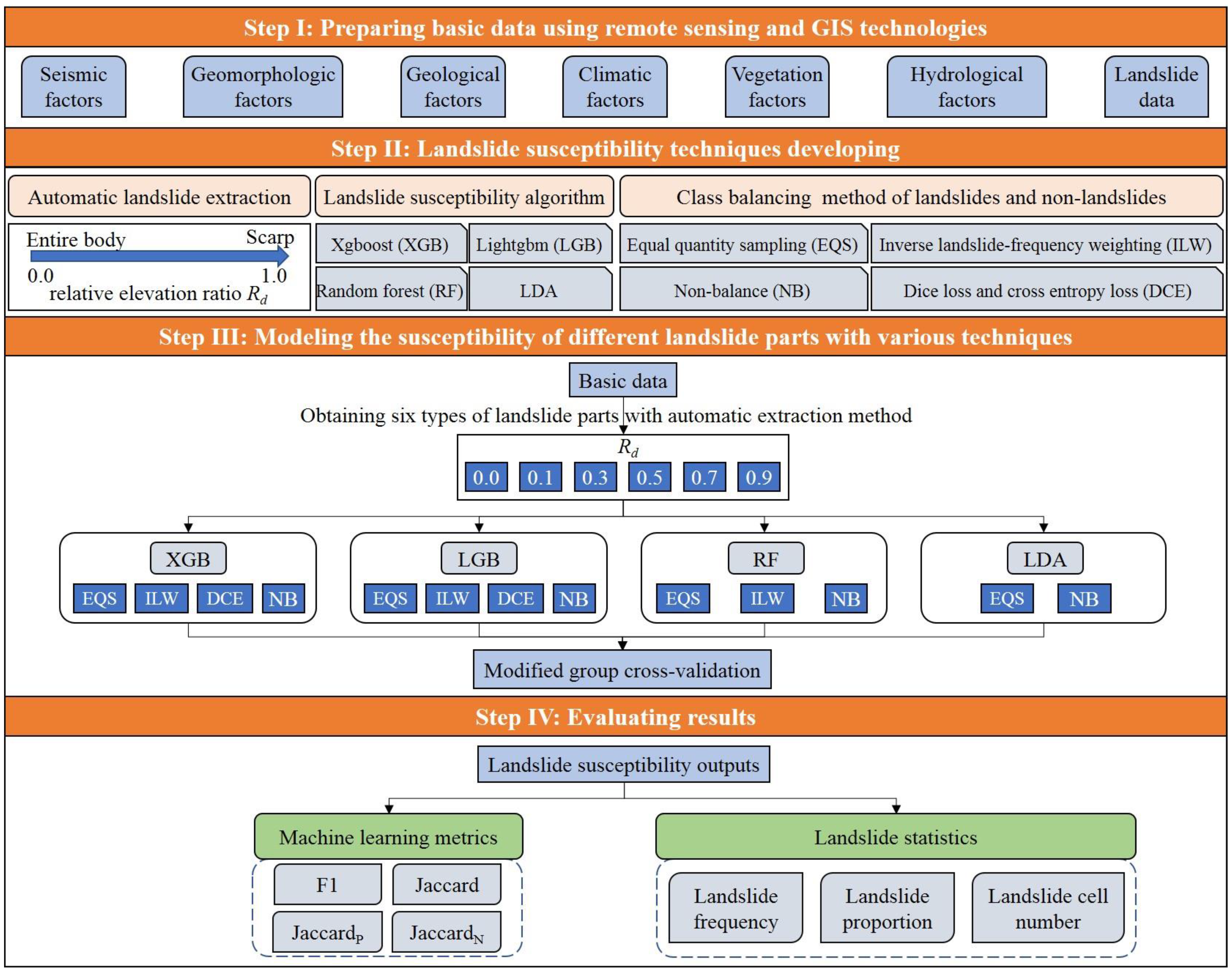
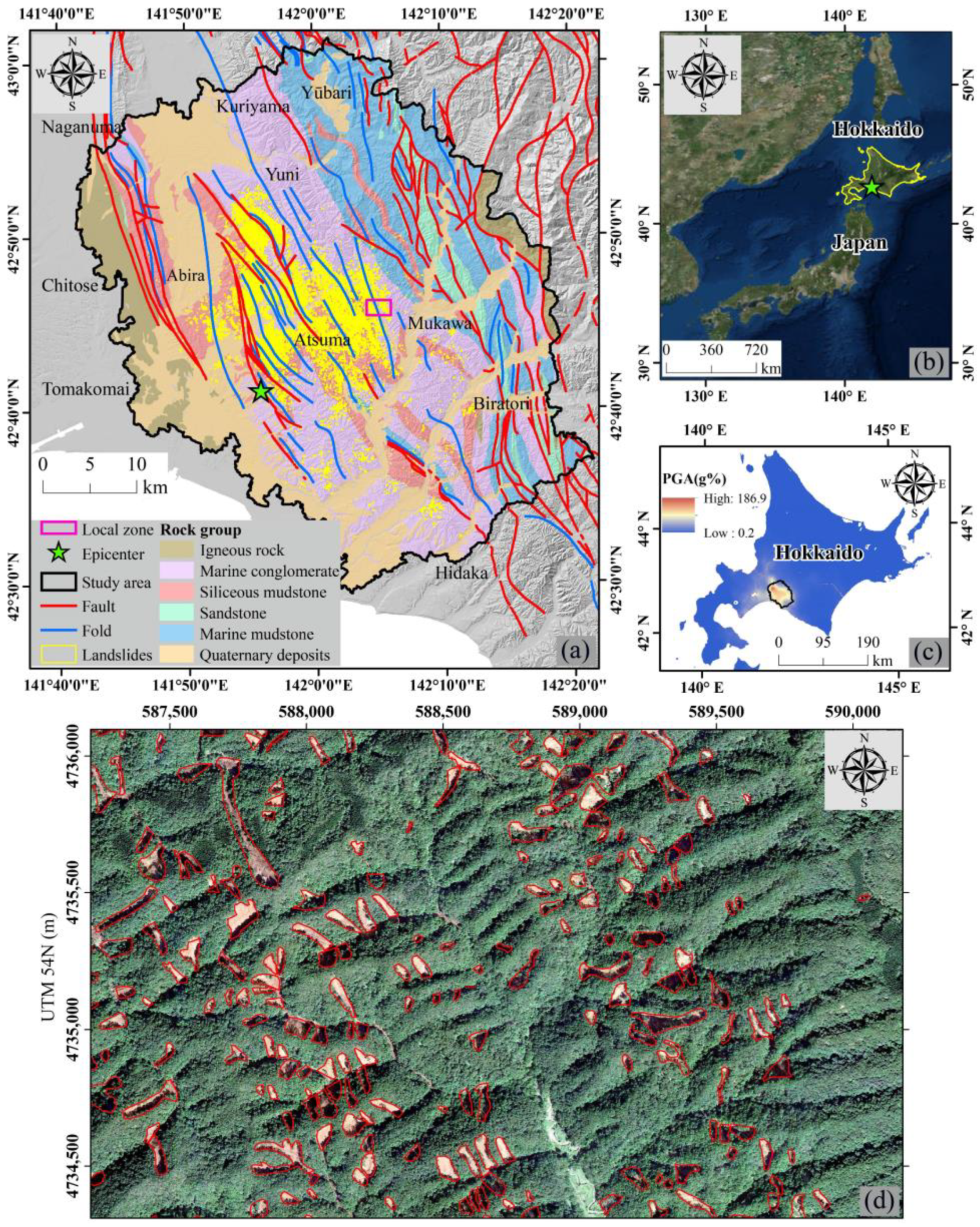
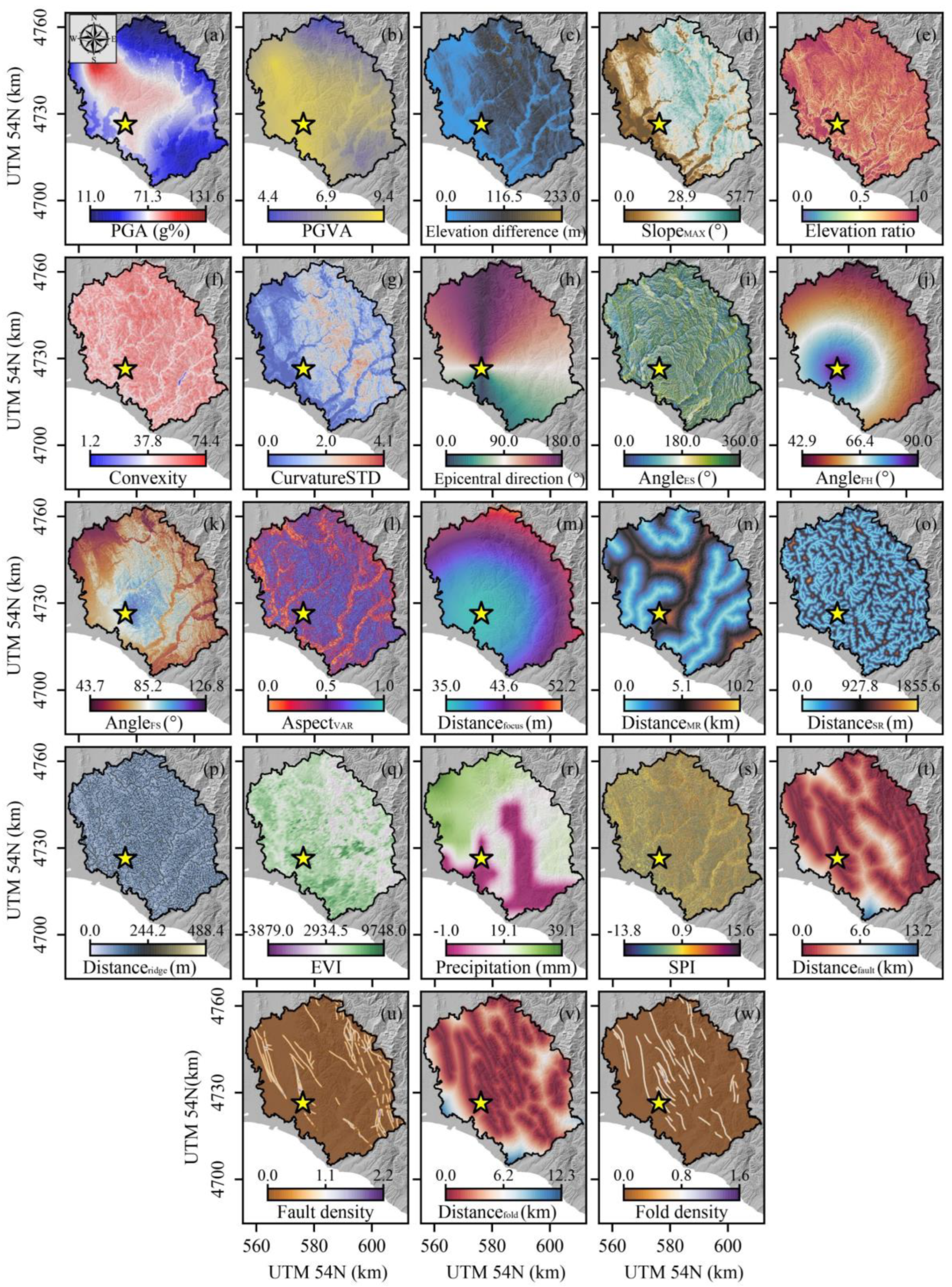
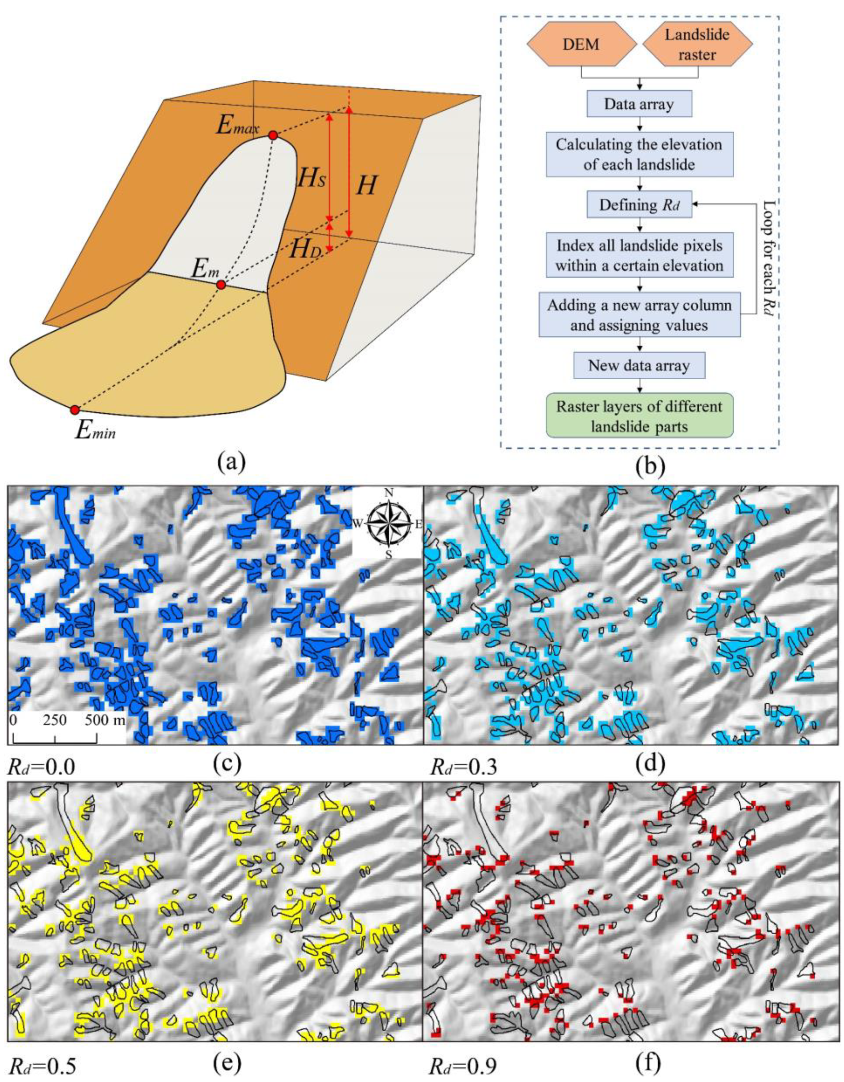
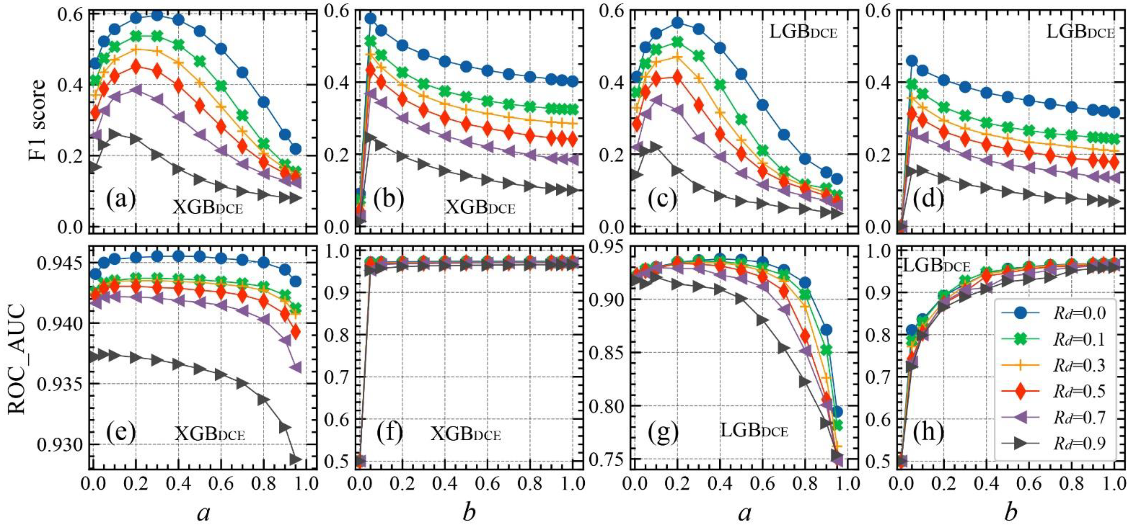
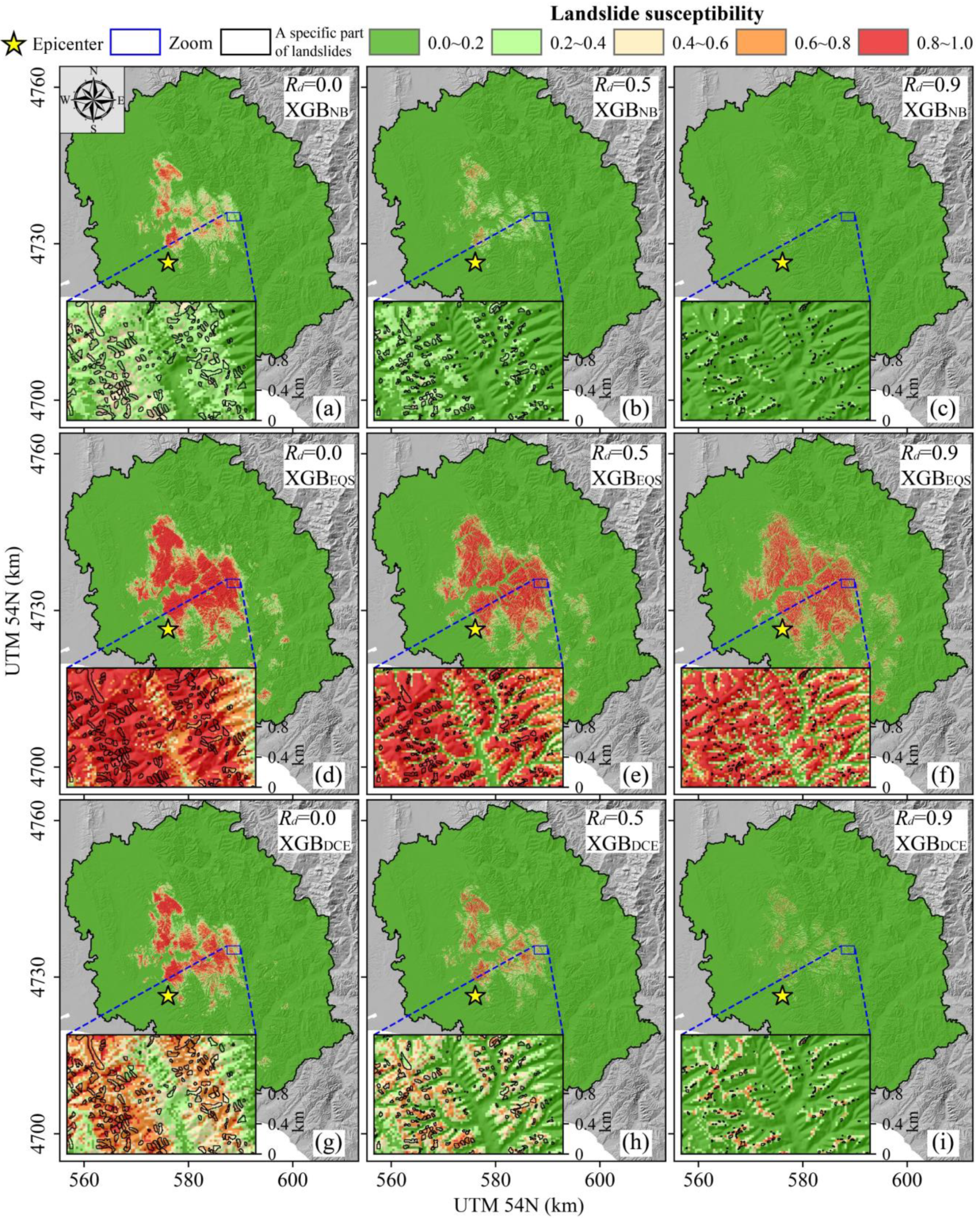
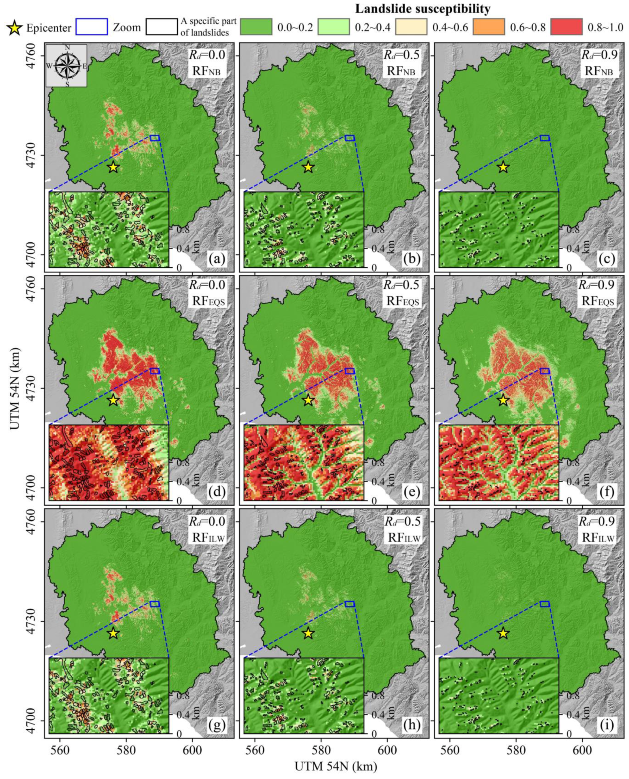
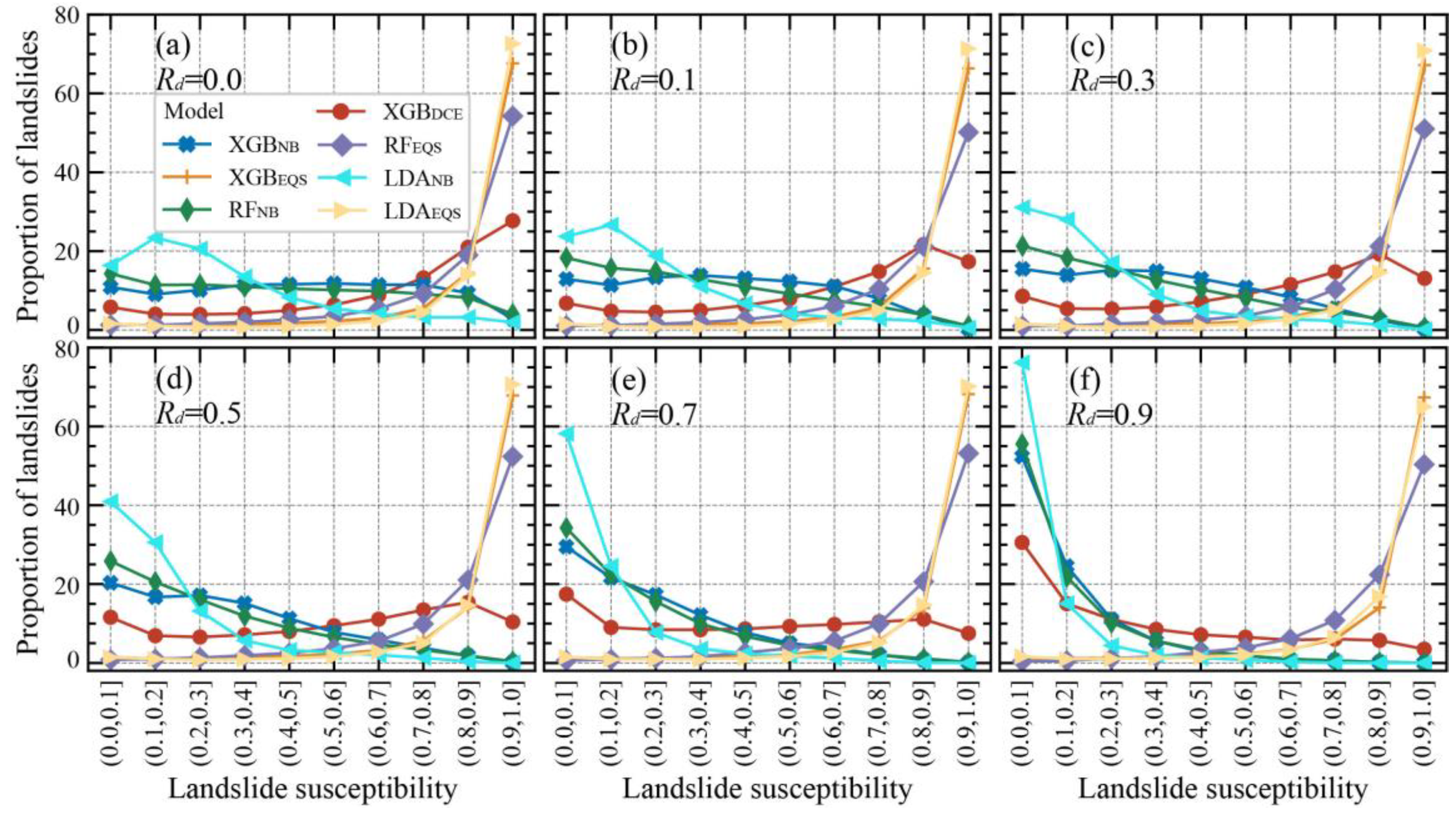
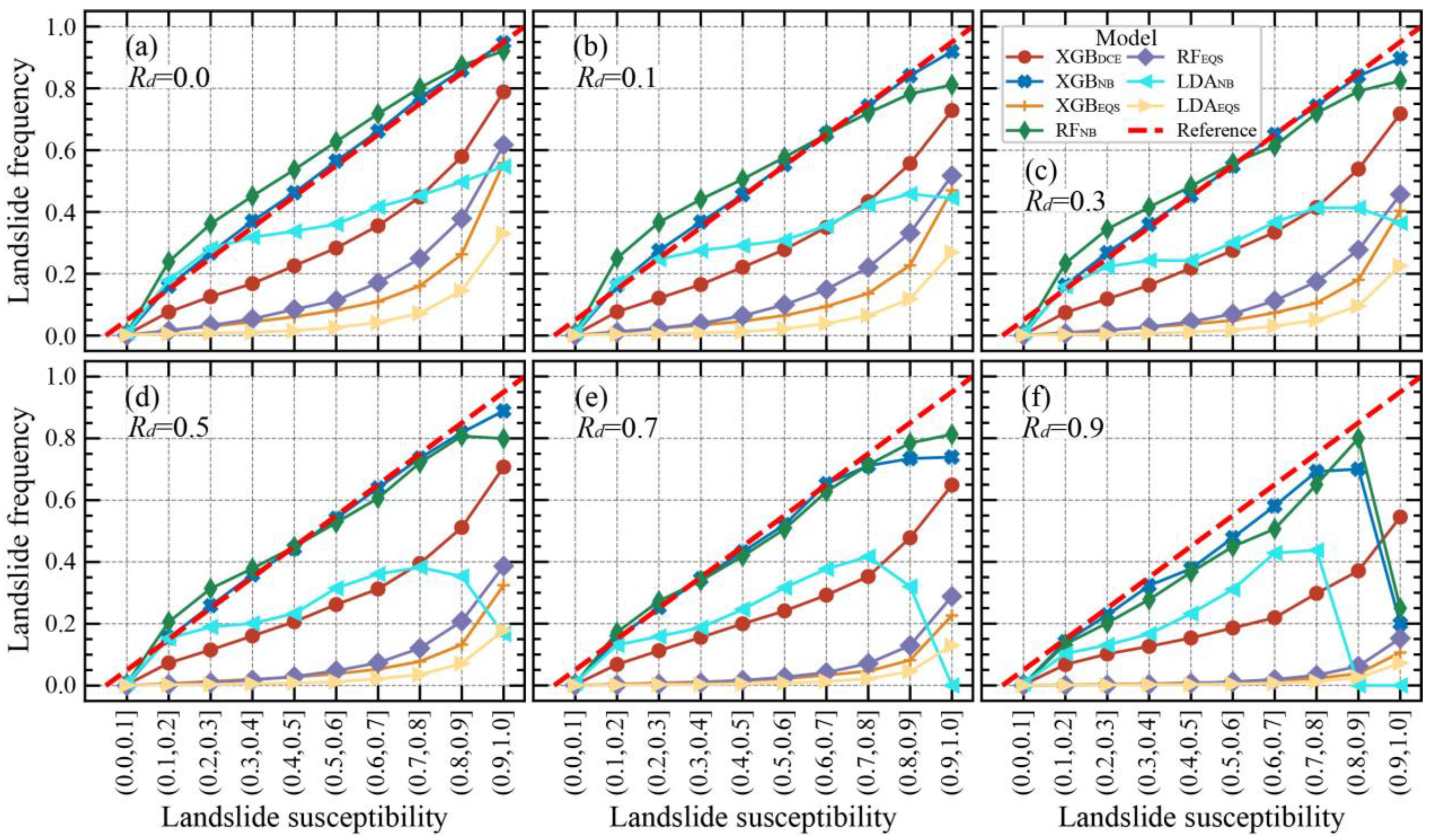
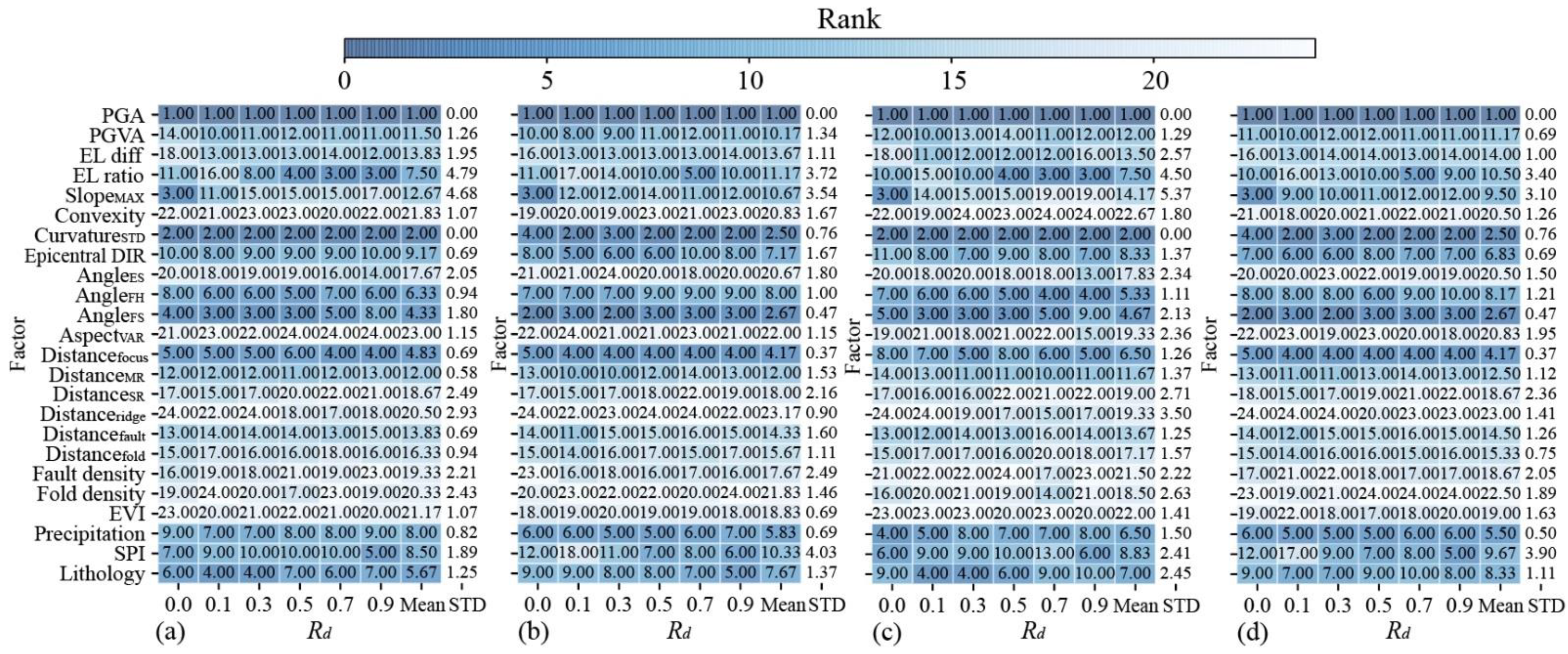
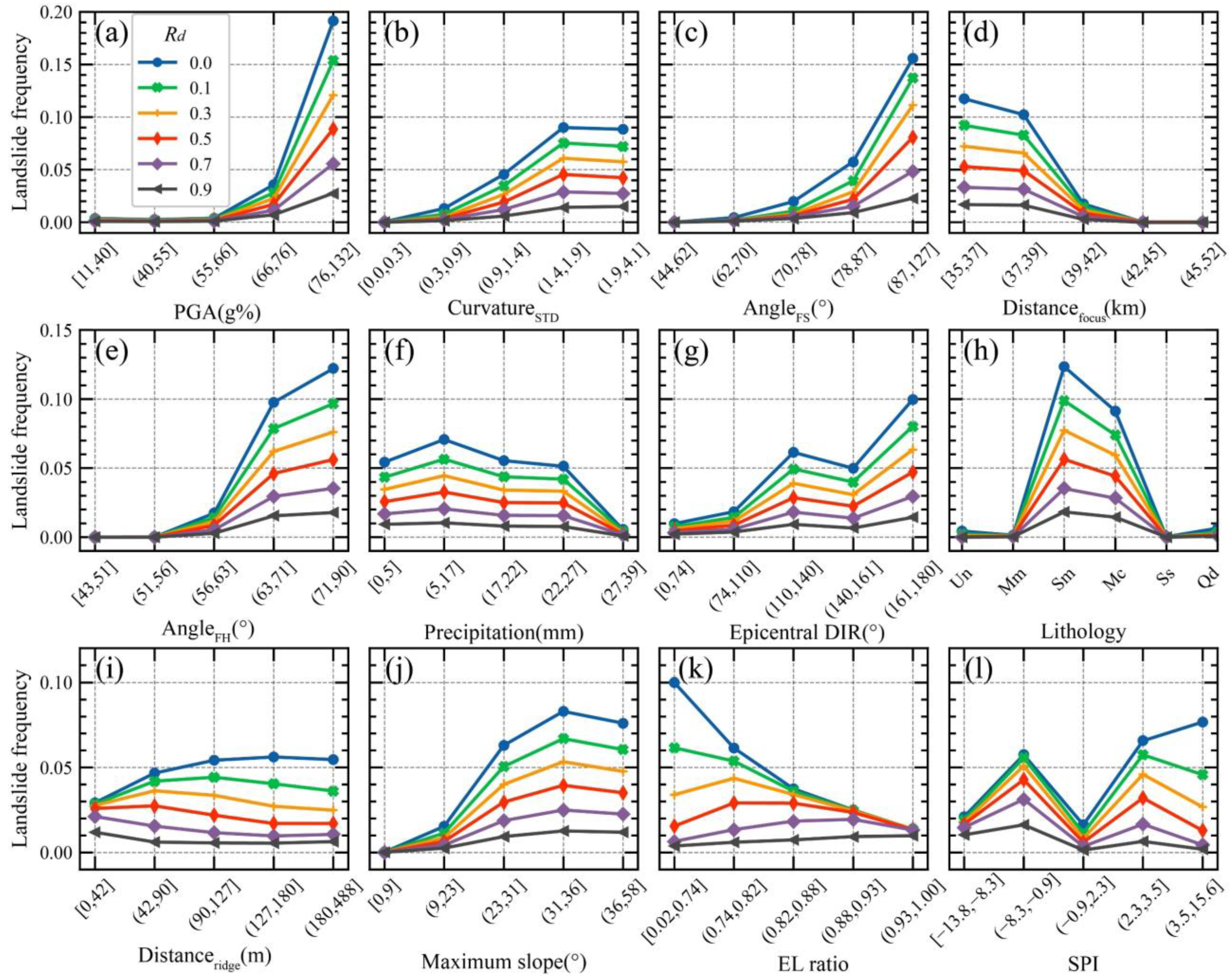
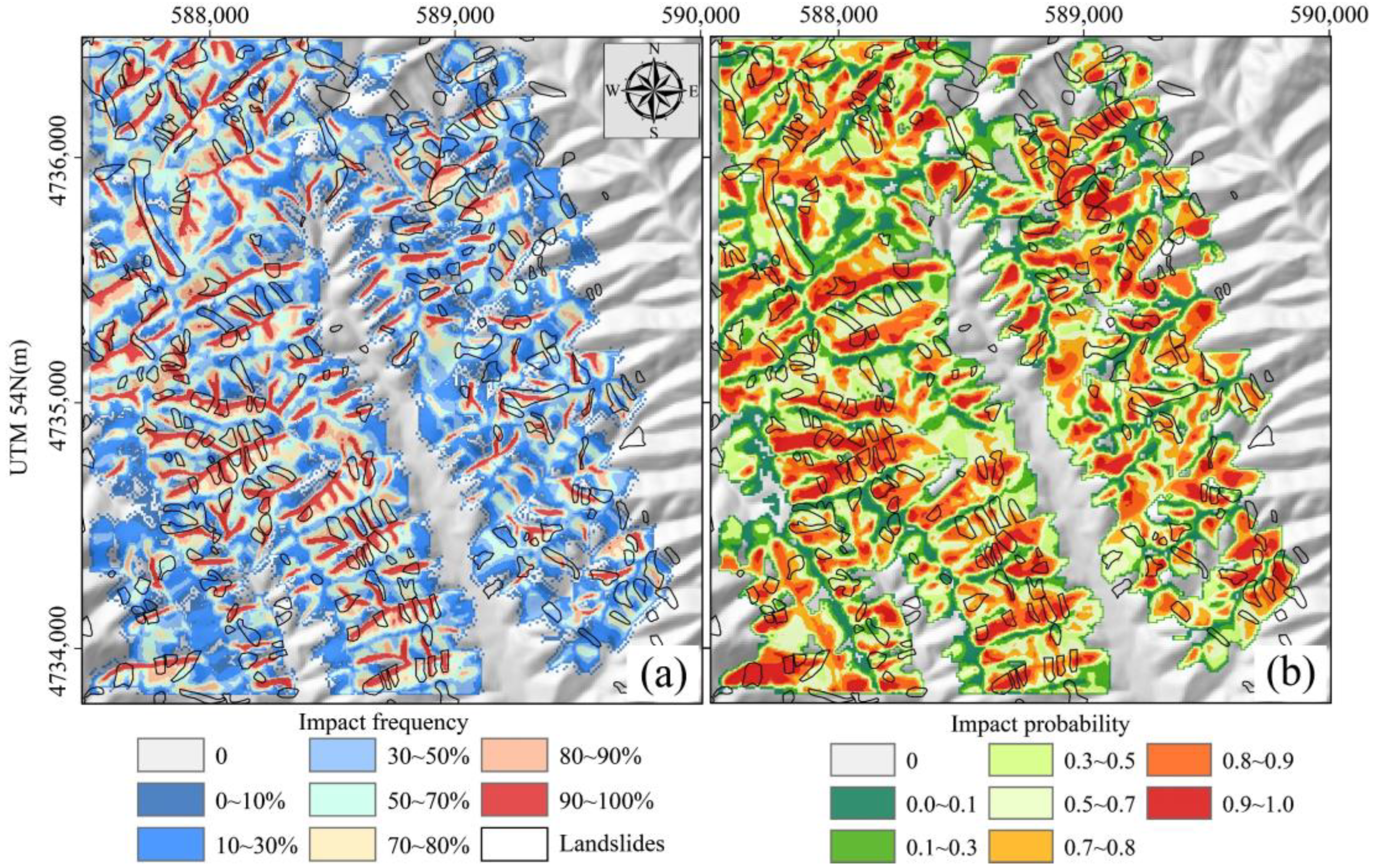
Table 1.
Data set sources and meta-data.
| Basic Data | Source | Date | Resolution |
|---|---|---|---|
| Digital elevation model (DEM) | Geospatial Authority Institute of Japan (https://fgd.gsi.go.jp/download/menu.php accessed on 1 September 2022) | 1 October 2016 | 10 m |
| QuiQuake | Geological Survey of Japan, AIST (https://gbank.gsj.jp/QuiQuake/QuakeMap/index.en.html accessed on 1 September 2022) | 6 September 2018 | 250 m |
| Shakemap | United States Geological Survey (USGS) (https://earthquake.usgs.gov/data/shakemap/ accessed on 1 September 2022) | 6 September 2018 | — |
| CHIRPS | Climate Hazards Center (https://www.chc.ucsb.edu/data/chirps accessed on 1 September 2022) | 3 September 2018–6 September 2018 | 5000 m |
| MODIS Vegetation Index | NASA (https://earthdata.nasa.gov/ accessed on 1 September 2022) | 13 August 2018–28 August 2018 | 250 m |
| Geological map | Geological Survey of Japan, AIST (https://gbank.gsj.jp/seamless/v2.html accessed on 1 September 2022) | 22 January 2021 | 1:200,000 |
| Google earth imagery | Google earth pro | 30 September 2016–10 July 2020 | 0.2 m |
| Aerial photos | Geospatial Authority Institute of Japan (https://kmlnetworklink.gsi.go.jp/kmlnetworklink/index.html accessed on 1 September 2022) | 6 September 2018–13 September 2018 | 0.2 m |
QuiQuake = Quick estimation system for earthquake maps triggered by observation records; CHIRPS = Climate Hazards Group InfraRed Precipitation with Station data.
Table 2.
Description of factors influencing landslides.
| Type | Factor | Basic Data | Range | Unit | Resolution |
|---|---|---|---|---|---|
| Seismic | Peak ground acceleration (PGA) | QuiQuake | 11.0–131.6 | g% | 250 m |
| PGVA, the product of PGV (peak ground velocity) and PGA | 4.4–9.4 | — | 250 m | ||
| The Euclidean distance to the focus (distancefocus) | Shakemap | 35.0–52.2 | km | 30 m | |
| Epicentral direction | 0.0–180.0 | ° | 30 m | ||
| The Euclidean distance to the nearest ridge (distanceridge) | DEM | 0.0–488.4 | m | 30 m | |
| The angle between epicentral direction and the slope aspect (angleES) | DEM and QuiQuake | 0.0–360.0 | ° | 30 m | |
| The angle between the horizontal and the line from calculated cell to focus (angleFH). AngleFH represents the direction of seismic wave propagation at a location, which would influence the occurrence of landslides. | 42.9–90.0 | ° | 30 m | ||
| The sum of angleFH and the slope degree (angleFS) | 43.7–126.8 | ° | 30 m | ||
| Geomorphologic | The maximum slope in the neighbourhood of the calculated cell (slopeMAX) | DEM | 0.0–57.7 | ° | 30 m |
| The variation of the slope aspects in the neighbourhood of the calculated cell (aspectVAR) | 0.0–1.0 | — | 30 m | ||
| The ratio of the elevation to the maximum elevation in the neighbourhood of the calculated cell (elevation ratio) | 0.0–1.0 | — | 30 m | ||
| Elevation difference | 0.0–233.0 | m | 30 m | ||
| The percentage of convex cells in the neighbourhood of the calculated cell (surface convexity) [43]. Surface convexity describes the shape (convex, concave, flat) of the slope, which affects the stability of the slope under earthquake shaking. | 1.2–74.4 | — | 30 m | ||
| The standard deviation of the curvature in the neighbourhood of the calculated cell (curvatureSTD) | 0.0–4.1 | — | 30 m | ||
| Hydrological | The shortest Euclidean distance to minor rivers (distanceSR) | DEM | 0.0–1855.6 | m | 30 m |
| The shortest Euclidean distance to major rivers (distanceMR) | 0.0–10.2 | km | 30 m | ||
| Stream power index (SPI) | −13.8–15.6 | — | 30 m | ||
| Climatic | Cumulative precipitation in the 4 days before an earthquake (precipitation) | CHIRPS | 0.0–39.1 | mm | 5000 m |
| Vegetation cover | Enhanced vegetation index (EVI) | MODIS Vegetation Index Products | −3879.0–9748.0 | — | 250 m |
| Geological | Lithology | Geological map | — | — | — |
| The Euclidean distance to the nearest fault (distancefault) | 0.0–13.2 | km | 30 m | ||
| The Euclidean distance to the nearest fold (distancefold) | 0.0–12.3 | km | 30 m | ||
| Fault density (LF × WF/AF). LF, WF, and AF are the total fault length, fault width, and area of the statistical zone, respectively. | 0.0–2.2 | — | 30 m | ||
| Fold density (LO × WO/AO). LO, WO, and AO are the total fold length, fold width, and area of the statistical zone, respectively. | 0.0–1.6 | — | 30 m |
Table 3.
Inventories of different landslide parts.
| Rd | Number of Landslide Parts | Number of Landslide Cells | Number of Non-landslide Cells | Ratio of Landslide to Non-Landslide | Area of Landslide Cells | Total Study Area (km2) | Landslide Frequency | |
|---|---|---|---|---|---|---|---|---|
| Sum (km2) | Mean (m2) | |||||||
| 0.0 | 10,422 | 10,4826 | 2,101,479 | 1:20 | 94.34 | 9052.33 | 1985.67 | 0.048 |
| 0.1 | 10,422 | 83,663 | 2,122,642 | 1:25 | 75.30 | 7224.78 | 1985.67 | 0.038 |
| 0.3 | 10,422 | 66,120 | 2,140,185 | 1:32 | 59.51 | 5709.84 | 1985.67 | 0.030 |
| 0.5 | 10,422 | 48,864 | 2,157,441 | 1:44 | 43.98 | 4219.69 | 1985.67 | 0.022 |
| 0.7 | 10,422 | 31,152 | 2,175,153 | 1:70 | 28.04 | 2690.16 | 1985.67 | 0.014 |
| 0.9 | 10,422 | 16,061 | 2,190,244 | 1:136 | 14.45 | 1386.96 | 1985.67 | 0.007 |
Landslide frequency: the ratio of the sum of the areas of the landslide parts to the total study area.
Table 4.
Model prediction performance of different landslide features for every model.
| Model | Rd = 0.0 | Rd = 0.1 | ||||||||||||||
|---|---|---|---|---|---|---|---|---|---|---|---|---|---|---|---|---|
| PRE | REC | F1 | JACP | JACN | JAC | AUC | Freq | PRE | REC | F1 | JACP | JACN | JAC | AUC | Freq | |
| XGBNB | 0.699 | 0.468 | 0.561 | 0.390 | 0.964 | 0.613 | 0.974 | 0.048 | 0.646 | 0.354 | 0.457 | 0.297 | 0.968 | 0.536 | 0.971 | 0.038 |
| XGBEQS | 0.350 | 0.930 | 0.509 | 0.341 | 0.911 | 0.557 | 0.972 | 0.048 | 0.290 | 0.932 | 0.442 | 0.284 | 0.908 | 0.508 | 0.970 | 0.038 |
| XGBILW | 0.366 | 0.916 | 0.523 | 0.354 | 0.917 | 0.570 | 0.972 | 0.048 | 0.307 | 0.916 | 0.460 | 0.299 | 0.916 | 0.523 | 0.970 | 0.038 |
| XGBDCE | 0.520 | 0.771 | 0.621 | 0.451 | 0.954 | 0.655 | 0.973 | 0.048 | 0.464 | 0.727 | 0.566 | 0.395 | 0.957 | 0.615 | 0.971 | 0.038 |
| LGBNB | 0.639 | 0.429 | 0.512 | 0.344 | 0.960 | 0.575 | 0.968 | 0.048 | 0.594 | 0.290 | 0.389 | 0.242 | 0.965 | 0.483 | 0.966 | 0.038 |
| LGBEQS | 0.320 | 0.942 | 0.477 | 0.313 | 0.897 | 0.530 | 0.971 | 0.048 | 0.266 | 0.945 | 0.415 | 0.262 | 0.895 | 0.484 | 0.969 | 0.038 |
| LGBILW | 0.322 | 0.941 | 0.480 | 0.316 | 0.898 | 0.532 | 0.971 | 0.048 | 0.268 | 0.944 | 0.418 | 0.264 | 0.897 | 0.486 | 0.969 | 0.038 |
| LGBDCE | 0.471 | 0.797 | 0.592 | 0.421 | 0.946 | 0.631 | 0.970 | 0.048 | 0.419 | 0.760 | 0.540 | 0.370 | 0.949 | 0.592 | 0.968 | 0.038 |
| RFNB | 0.751 | 0.414 | 0.534 | 0.364 | 0.965 | 0.593 | 0.969 | 0.048 | 0.656 | 0.274 | 0.387 | 0.240 | 0.967 | 0.481 | 0.963 | 0.038 |
| RFEQS | 0.387 | 0.912 | 0.543 | 0.373 | 0.924 | 0.587 | 0.972 | 0.048 | 0.320 | 0.915 | 0.475 | 0.311 | 0.920 | 0.535 | 0.969 | 0.038 |
| RFILW | 0.751 | 0.379 | 0.504 | 0.337 | 0.964 | 0.570 | 0.963 | 0.048 | 0.652 | 0.247 | 0.358 | 0.218 | 0.966 | 0.459 | 0.957 | 0.038 |
| LDANB | 0.426 | 0.178 | 0.251 | 0.144 | 0.949 | 0.369 | 0.925 | 0.048 | 0.367 | 0.129 | 0.191 | 0.106 | 0.958 | 0.318 | 0.922 | 0.038 |
| LDAEQS | 0.194 | 0.949 | 0.322 | 0.192 | 0.802 | 0.393 | 0.936 | 0.048 | 0.157 | 0.950 | 0.270 | 0.156 | 0.798 | 0.353 | 0.932 | 0.038 |
| Model | Rd= 0.3 | Rd= 0.5 | ||||||||||||||
| PRE | REC | F1 | JACP | JACN | JAC | AUC | Freq | PRE | REC | F1 | JACP | JACN | JAC | AUC | Freq | |
| XGBNB | 0.631 | 0.274 | 0.382 | 0.236 | 0.973 | 0.479 | 0.971 | 0.030 | 0.623 | 0.198 | 0.301 | 0.177 | 0.980 | 0.416 | 0.971 | 0.022 |
| XGBEQS | 0.240 | 0.931 | 0.382 | 0.236 | 0.907 | 0.463 | 0.969 | 0.030 | 0.183 | 0.932 | 0.305 | 0.180 | 0.904 | 0.404 | 0.968 | 0.022 |
| XGBILW | 0.260 | 0.913 | 0.404 | 0.253 | 0.917 | 0.482 | 0.970 | 0.030 | 0.206 | 0.906 | 0.335 | 0.201 | 0.919 | 0.430 | 0.970 | 0.022 |
| XGBDCE | 0.431 | 0.677 | 0.527 | 0.357 | 0.963 | 0.587 | 0.971 | 0.030 | 0.398 | 0.598 | 0.478 | 0.314 | 0.971 | 0.552 | 0.971 | 0.022 |
| LGBNB | 0.480 | 0.212 | 0.280 | 0.163 | 0.965 | 0.395 | 0.960 | 0.030 | 0.480 | 0.140 | 0.214 | 0.120 | 0.977 | 0.342 | 0.964 | 0.022 |
| LGBEQS | 0.222 | 0.945 | 0.359 | 0.219 | 0.896 | 0.443 | 0.969 | 0.030 | 0.171 | 0.942 | 0.289 | 0.169 | 0.895 | 0.389 | 0.969 | 0.022 |
| LGBILW | 0.225 | 0.943 | 0.364 | 0.222 | 0.898 | 0.447 | 0.969 | 0.030 | 0.176 | 0.939 | 0.297 | 0.174 | 0.899 | 0.396 | 0.969 | 0.022 |
| LGBDCE | 0.391 | 0.709 | 0.504 | 0.337 | 0.957 | 0.568 | 0.968 | 0.030 | 0.351 | 0.632 | 0.452 | 0.292 | 0.966 | 0.531 | 0.967 | 0.022 |
| RFNB | 0.633 | 0.218 | 0.324 | 0.193 | 0.973 | 0.434 | 0.961 | 0.030 | 0.610 | 0.168 | 0.263 | 0.152 | 0.979 | 0.385 | 0.958 | 0.022 |
| RFEQS | 0.263 | 0.919 | 0.409 | 0.257 | 0.918 | 0.486 | 0.969 | 0.030 | 0.197 | 0.925 | 0.325 | 0.194 | 0.913 | 0.421 | 0.969 | 0.022 |
| RFILW | 0.624 | 0.195 | 0.298 | 0.175 | 0.972 | 0.412 | 0.953 | 0.030 | 0.604 | 0.153 | 0.244 | 0.139 | 0.979 | 0.369 | 0.950 | 0.022 |
| LDANB | 0.354 | 0.099 | 0.154 | 0.084 | 0.967 | 0.284 | 0.921 | 0.030 | 0.344 | 0.064 | 0.108 | 0.057 | 0.977 | 0.236 | 0.922 | 0.022 |
| LDAEQS | 0.126 | 0.949 | 0.223 | 0.125 | 0.796 | 0.316 | 0.932 | 0.030 | 0.095 | 0.947 | 0.173 | 0.094 | 0.795 | 0.274 | 0.933 | 0.022 |
| Model | Rd= 0.7 | Rd= 0.9 | ||||||||||||||
| PRE | REC | F1 | JACP | JACN | JAC | AUC | Freq | PRE | REC | F1 | JACP | JACN | JAC | AUC | Freq | |
| XGBNB | 0.602 | 0.117 | 0.196 | 0.109 | 0.986 | 0.328 | 0.970 | 0.014 | 0.555 | 0.034 | 0.064 | 0.033 | 0.993 | 0.181 | 0.965 | 0.007 |
| XGBEQS | 0.117 | 0.932 | 0.208 | 0.116 | 0.899 | 0.323 | 0.967 | 0.014 | 0.055 | 0.932 | 0.105 | 0.055 | 0.883 | 0.221 | 0.960 | 0.007 |
| XGBILW | 0.139 | 0.898 | 0.241 | 0.137 | 0.919 | 0.354 | 0.968 | 0.014 | 0.072 | 0.874 | 0.133 | 0.071 | 0.916 | 0.255 | 0.963 | 0.007 |
| XGBDCE | 0.353 | 0.481 | 0.407 | 0.255 | 0.980 | 0.500 | 0.970 | 0.014 | 0.266 | 0.277 | 0.271 | 0.157 | 0.989 | 0.394 | 0.965 | 0.007 |
| LGBNB | 0.396 | 0.120 | 0.182 | 0.100 | 0.985 | 0.314 | 0.963 | 0.014 | 0.226 | 0.060 | 0.093 | 0.049 | 0.991 | 0.218 | 0.953 | 0.007 |
| LGBEQS | 0.111 | 0.941 | 0.199 | 0.110 | 0.892 | 0.314 | 0.968 | 0.014 | 0.054 | 0.937 | 0.102 | 0.054 | 0.879 | 0.217 | 0.962 | 0.007 |
| LGBILW | 0.117 | 0.935 | 0.207 | 0.116 | 0.898 | 0.322 | 0.969 | 0.014 | 0.058 | 0.929 | 0.109 | 0.058 | 0.889 | 0.227 | 0.963 | 0.007 |
| LGBDCE | 0.288 | 0.511 | 0.366 | 0.225 | 0.974 | 0.466 | 0.963 | 0.014 | 0.230 | 0.296 | 0.259 | 0.149 | 0.988 | 0.383 | 0.959 | 0.007 |
| RFNB | 0.598 | 0.111 | 0.187 | 0.103 | 0.986 | 0.319 | 0.952 | 0.014 | 0.500 | 0.035 | 0.066 | 0.034 | 0.993 | 0.184 | 0.932 | 0.007 |
| RFEQS | 0.123 | 0.931 | 0.217 | 0.122 | 0.904 | 0.331 | 0.968 | 0.014 | 0.056 | 0.936 | 0.106 | 0.056 | 0.884 | 0.222 | 0.963 | 0.007 |
| RFILW | 0.580 | 0.100 | 0.170 | 0.093 | 0.986 | 0.303 | 0.941 | 0.014 | 0.495 | 0.031 | 0.059 | 0.030 | 0.993 | 0.174 | 0.916 | 0.007 |
| LDANB | 0.348 | 0.035 | 0.064 | 0.033 | 0.985 | 0.181 | 0.923 | 0.014 | 0.340 | 0.011 | 0.021 | 0.011 | 0.993 | 0.103 | 0.916 | 0.007 |
| LDAEQS | 0.062 | 0.944 | 0.116 | 0.061 | 0.794 | 0.221 | 0.934 | 0.014 | 0.031 | 0.936 | 0.060 | 0.031 | 0.787 | 0.157 | 0.930 | 0.007 |
Freq: landslide frequency. PRE: precision. F1:F1 score. JACP: JaccardP. JACN: JaccardN. JAC: Jaccard.
Table 5.
Statistical analysis of the number of cells (unit: thousand) in the generated landslide susceptibility maps for every model.
Table 5.
Statistical analysis of the number of cells (unit: thousand) in the generated landslide susceptibility maps for every model.
| Rd = 0.0 | Rd = 0.3 | |||||||||||
|---|---|---|---|---|---|---|---|---|---|---|---|---|
| Model | Landslide Susceptibility | Freq | Landslide Susceptibility | Freq | ||||||||
| 0.0–0.2 | 0.2–0.4 | 0.4–0.6 | 0.6–0.8 | 0.8–1.0 | 0.0–0.2 | 0.2–0.4 | 0.4–0.6 | 0.6–0.8 | 0.8–1.0 | |||
| XGBNB | 2037.5 | 72.4 | 47.9 | 33.9 | 14.5 | 0.048 | 2094.2 | 64.3 | 32.2 | 13.3 | 2.2 | 0.030 |
| XGBEQS | 1821.0 | 76.9 | 57.9 | 65.8 | 184.8 | 0.048 | 1840.1 | 78.5 | 57.5 | 64.8 | 165.4 | 0.030 |
| XGBILW | 1842.8 | 73.5 | 54.0 | 60.2 | 175.9 | 0.048 | 1874.6 | 72.0 | 52.4 | 57.2 | 150.1 | 0.030 |
| XGBDCE | 1969.0 | 58.8 | 46.7 | 57.0 | 74.8 | 0.048 | 2027.6 | 53.1 | 43.3 | 46.3 | 36.0 | 0.030 |
| LGBNB | 2023.4 | 87.0 | 53.5 | 36.3 | 6.0 | 0.048 | 2087.6 | 74.3 | 31.1 | 11.1 | 2.1 | 0.030 |
| LGBEQS | 1752.6 | 105.7 | 72.8 | 78.7 | 196.5 | 0.048 | 1778.1 | 104.4 | 73.4 | 75.8 | 174.5 | 0.030 |
| LGBILW | 1752.7 | 104.9 | 73.4 | 78.6 | 196.6 | 0.048 | 1782.2 | 105.4 | 72.6 | 74.4 | 171.7 | 0.030 |
| LGBDCE | 1929.9 | 70.5 | 58.2 | 74.7 | 73.0 | 0.048 | 1997.8 | 62.4 | 53.7 | 62.3 | 30.1 | 0.030 |
| RFNB | 2069.3 | 58.8 | 37.4 | 26.3 | 14.4 | 0.048 | 2119.2 | 50.3 | 23.6 | 10.3 | 2.9 | 0.030 |
| RFEQS | 1834.9 | 90.7 | 64.6 | 71.3 | 144.8 | 0.048 | 1829.5 | 107.2 | 71.8 | 73.4 | 124.4 | 0.030 |
| RFILW | 2078.9 | 55.0 | 35.5 | 24.9 | 12.0 | 0.048 | 2128.9 | 44.0 | 21.5 | 9.6 | 2.3 | 0.030 |
| LDANB | 2015.5 | 121.1 | 41.6 | 17.6 | 10.5 | 0.048 | 2099.2 | 75.4 | 20.9 | 8.6 | 2.3 | 0.030 |
| LDAEQS | 1448.9 | 181.9 | 120.7 | 122.6 | 332.2 | 0.048 | 1466.4 | 178.0 | 125.7 | 127.2 | 309.0 | 0.030 |
| Rd= 0.5 | Rd= 0.9 | |||||||||||
| Model | 0.0–0.2 | 0.2–0.4 | 0.4–0.6 | 0.6–0.8 | 0.8–1.0 | Freq | 0.0–0.2 | 0.2–0.4 | 0.4–0.6 | 0.6–0.8 | 0.8–1.0 | Freq |
| XGBNB | 2125.9 | 52.5 | 19.5 | 7.1 | 1.2 | 0.022 | 2193.4 | 10.7 | 1.8 | 0.4 | 0.0 | 0.007 |
| XGBEQS | 1845.8 | 81.9 | 59.3 | 64.9 | 154.4 | 0.022 | 1800.5 | 96.0 | 71.1 | 78.6 | 160.1 | 0.007 |
| XGBILW | 1890.5 | 73.1 | 52.3 | 56.6 | 133.7 | 0.022 | 1902.7 | 78.4 | 57.8 | 62.9 | 104.5 | 0.007 |
| XGBDCE | 2064.4 | 49.5 | 36.5 | 34.0 | 21.9 | 0.022 | 2153.8 | 28.3 | 13.1 | 7.5 | 3.5 | 0.007 |
| LGBNB | 2125.7 | 56.6 | 14.7 | 5.8 | 3.6 | 0.022 | 2193.4 | 8.3 | 1.4 | 0.8 | 2.3 | 0.007 |
| LGBEQS | 1784.3 | 112.6 | 75.4 | 74.9 | 159.1 | 0.022 | 1743.0 | 131.0 | 89.4 | 95.2 | 147.6 | 0.007 |
| LGBILW | 1794.6 | 109.4 | 74.3 | 73.5 | 154.5 | 0.022 | 1779.5 | 122.0 | 82.3 | 91.5 | 131.0 | 0.007 |
| LGBDCE | 2036.4 | 57.6 | 47.1 | 45.6 | 19.7 | 0.022 | 2141.5 | 34.9 | 16.3 | 9.7 | 3.9 | 0.007 |
| RFNB | 2142.9 | 40.4 | 15.7 | 6.0 | 1.4 | 0.022 | 2192.4 | 11.3 | 2.1 | 0.4 | 0.0 | 0.007 |
| RFEQS | 1814.0 | 120.7 | 79.3 | 76.8 | 115.5 | 0.022 | 1696.1 | 180.2 | 115.5 | 103.6 | 110.9 | 0.007 |
| RFILW | 2150.4 | 34.8 | 14.4 | 5.6 | 1.1 | 0.022 | 2194.1 | 9.9 | 1.8 | 0.4 | 0.0 | 0.007 |
| LDANB | 2142.7 | 47.8 | 11.0 | 4.4 | 0.5 | 0.022 | 2197.6 | 7.4 | 1.3 | 0.1 | 0.0 | 0.007 |
| LDAEQS | 1466.6 | 184.8 | 129.7 | 132.6 | 292.5 | 0.022 | 1436.9 | 210.0 | 148.3 | 158.5 | 252.6 | 0.007 |
Freq: landslide frequency.
Publisher’s Note: MDPI stays neutral with regard to jurisdictional claims in published maps and institutional affiliations. |
© 2022 by the authors. Licensee MDPI, Basel, Switzerland. This article is an open access article distributed under the terms and conditions of the Creative Commons Attribution (CC BY) license (https://creativecommons.org/licenses/by/4.0/).
Share and Cite
MDPI and ACS Style
Zhang, S.; Wang, Y.; Wu, G. Earthquake-Induced Landslide Susceptibility Assessment Using a Novel Model Based on Gradient Boosting Machine Learning and Class Balancing Methods. Remote Sens. 2022, 14, 5945. https://doi.org/10.3390/rs14235945
AMA Style
Zhang S, Wang Y, Wu G. Earthquake-Induced Landslide Susceptibility Assessment Using a Novel Model Based on Gradient Boosting Machine Learning and Class Balancing Methods. Remote Sensing. 2022; 14(23):5945. https://doi.org/10.3390/rs14235945
Chicago/Turabian StyleZhang, Shuhao, Yawei Wang, and Guang Wu. 2022. "Earthquake-Induced Landslide Susceptibility Assessment Using a Novel Model Based on Gradient Boosting Machine Learning and Class Balancing Methods" Remote Sensing 14, no. 23: 5945. https://doi.org/10.3390/rs14235945
Note that from the first issue of 2016, this journal uses article numbers instead of page numbers. See further details here.