
Advances in Hyperspectral Image Classification Methods with Small Samples: A Review

1
College of Astronautics, Nanjing University of Aeronautics and Astronautics, Nanjing 210016, China
2
Beijing Institute of Space Mechanics & Electricity, Beijing 100094, China
*
Author to whom correspondence should be addressed.
Remote Sens. 2023, 15(15), 3795; https://doi.org/10.3390/rs15153795
Submission received: 18 June 2023
/
Revised: 22 July 2023
/
Accepted: 26 July 2023
/
Published: 30 July 2023
(This article belongs to the Section AI Remote Sensing)
Abstract
:Hyperspectral image (HSI) classification is one of the hotspots in remote sensing, and many methods have been continuously proposed in recent years. However, it is still challenging to achieve high accuracy classification in applications. One of the main reasons is the lack of labeled data. Due to the limitation of spatial resolution, manual labeling of HSI data is time-consuming and costly, so it is difficult to obtain a large amount of labeled data. In such a situation, many researchers turn their attention to the study of HSI classification with small samples. Focusing on this topic, this paper provides a systematic review of the research progress in recent years. Specifically, this paper contains three aspects. First, considering that the taxonomy used in previous review articles is not well-developed and confuses the reader, we propose a novel taxonomy based on the form of data utilization. This taxonomy provides a more accurate and comprehensive framework for categorizing the various approaches. Then, using the proposed taxonomy as a guideline, we analyze and summarize the existing methods, especially the latest research results (both deep and non-deep models) that were not included in the previous reviews, so that readers can understand the latest progress more clearly. Finally, we conduct several sets of experiments and present our opinions on current problems and future directions.
1. Introduction
Hyperspectral remote sensing is a powerful multidimensional information acquisition technology to detect both spatial and spectral information of the Earth’s surface [1,2]. The technology is widely used in various fields, including agricultural monitoring, resource exploration, and urban construction [3,4,5].
HSI classification is an important topic in hyperspectral remote sensing [6,7,8]. In the past five years, papers related to classification have occupied the main part of hyperspectral remote sensing research. HSI classification is the process of assigning semantic classes to each pixel using spectral features and spatial features [9]. Although related research is developing rapidly, achieving accurate classification of HSI is still a rather challenging task due to a number of reasons [10]. First, the process of acquiring HSI brings non-negligible negative effects for accurate classification. On the one hand, scattering can cause spectral mixing between different classes of adjacent image elements [11], and on the other hand, atmospheric aberrations and alignment deviations can also adversely affect the imaging process. Under these circumstances, samples of the same class sometimes exhibit different spectral qualities, which undoubtedly increases the difficulty of classification. In addition to the classification difficulty caused by the properties of HSI themselves, the limited number of labeled samples is also a key factor limiting classification accuracy.
For machine learning, there is a widely accepted consensus that the effectiveness of a model is positively correlated with the number of labeled samples [12]. This is because it is difficult for the model to infer regularity from the limited samples, resulting in poor generalization ability. It is easy to understand that more available samples are likely to provide more learnable knowledge when training classifiers, and make it easier to train a high-performing classifier. Especially with the rapid development of deep learning, more researchers intuitively realize the importance of the amount of labeled data in training models [13]. Deep learning models are known to be data-hungry, requiring large amounts of labeled data to fit their enormous parameter space. The success of deep learning is largely attributed to the availability of a massive amount of labeled data. Without a sufficient amount of labeled data, it may be difficult for even the best model to present full performance. However, obtaining labeled data is a challenging task in many fields, including hyperspectral remote sensing.
The spatial resolution of HSI is usually limited due to the irreconcilable conflict between spectral resolution and spatial resolution. In this case, the labeling of HSI cannot be completed solely by observing the images as in most data labeling in computer vision. Generally, this work requires field surveys and validation, and even the assistance of other data. For example, in 2020, the aerial hyperspectral remote sensing dataset of Xiongan New Area was released, and although its spatial resolution has reached 0.5 m, it is still labeled by field surveys combined with global position system (GPS) [14]. Therefore, HSI label acquisition is very time-consuming and expensive, and the currently available HSI label samples are very limited.
Achieving accurate classification of hyperspectral data with small samples is undoubtedly more challenging than with sufficient sample size. The prerequisite for a model obtained on a training set to perform well in testing is that the training set describes the true distribution of the data. Obviously, when the training samples are sufficient, the above condition is easier to fulfill. However, when the training samples are insufficient, the data distribution formed by a few training samples is more likely to be biased, which will result in the learned model being more prone to overfitting. In addition, considering that the high-dimensional features of hyperspectral images make the samples sparsely distributed in the feature space, the overfitting problem caused by insufficient samples will be more prominent. This is the main reason why hyperspectral images are currently difficult to classify with small samples.
Given the urgent need for accurate HSI classification techniques and the difficulty in obtaining labeled data, research on methods with a small labeled sample is essential. In fact, researchers have been aware of this need and have conducted research on it for more than a decade. Since 2008, more than one hundred papers have been published on the classification of HSI with small samples or limited data. At present, hyperspectral image classification with small samples (HIC-SS) has entered a period of rapid development. More than seventy percent of all related articles are from after 2018, and close to sixty percent are from after 2020.
In the early stage of research, some scholars focused on feature representation of HSI, and some feature extraction and feature selection methods were born as a result. Some examples are non-parametric weighted feature extraction [15], dimension reduction techniques [16], attraction points feature extraction [17], band clustering [18], etc. In addition, other researchers focus on designing more robust classifiers, such as classification methods based on sparse representation [19] and ensemble learning [20,21,22,23]. In later research, HIC-SS methods based on deep models gradually became mainstream. Among them, the use of convolutional neural networks (CNN) is undoubtedly revolutionary. The vast majority of methods used for HIC-SS are built on CNN [24,25,26,27,28,29,30,31,32,33]. Among these CNN-based approaches, some focus on extracting features with better differentiability from a limited samples [24,34,35,36], while others focus on optimizing the training process of classifiers [37]. The learning paradigms used cover a variety of models including self-supervised learning [38], transfer learning [39], active learning [40,41], meta-learning [37,42,43], and so on.
With the increasing number of relevant articles in the last five years, a review of these articles is very necessary. However, the fact is that the number of review articles on HIC-SS is very few [44,45,46]. Among them, the literature in [46] provides a systematic and comprehensive review of deep learning-based HIC-SS methods, which classifies and introduces a large number of existing methods and has an important reference value for subsequent research. Meanwhile, with the passage of time and the continuous development of technology, the review represented by [46] still needs to be supplemented and developed, which is mainly reflected in the following aspects.
- The current reviews categorize HIC-SS methods invariably according to the learning paradigm. However, some learning paradigms do not have a precise definition, especially those that have just been developed in recent years. The boundaries of these learning paradigms are ambiguous, and even the meaning of some learning paradigms has changed with further research. Therefore, there is some ambiguity in existing taxonomy based on learning paradigms in such cases.
- Most of the current reviews have focused on deep learning methods. Although deep models are the mainstream of current research, there are some non-deep models that have been proposed and have achieved remarkable results as well. In this case, it is necessary to provide a comprehensive overview of the research progress by taking non-deep models into account.
- Due to the rapid development of HIC-SS research, many more methods have been proposed in the past two years, and these methods were not mentioned in the previous reviews. In fact, the number of articles in this area is quite substantial. It is only by including them together that a more comprehensive understanding of the current developments in the field can be generated.
Based on the above reasons, we present a new overview of the research progress of HIC-SS. Notably, this paper does not use the learning paradigm as the taxonomy for method generalization, but generalizes the methods according to the form of data utilization. On this taxonomy, the boundaries between different methods are clearer and unnecessary ambiguities are also eliminated, which is conducive to the extraction and analysis of method generalities. In addition, on the basis of summarizing the existing methods, this paper also analyzes the problems faced by the existing methods through experiments and foresees future research trends.
The rest of the paper is organized as follows. Section 2 discusses in detail the limitations of using the learning paradigm as a basis for generalization and the taxonomy adopted in this paper. Section 3 reviews the current HIC-SS methods in detail. Section 4 provides a comparative description for the performance of the focused methods. Section 5 presents the perspectives. Section 6 concludes the paper.
2. Taxonomy
Taxonomy is a very important part of the review articles. As mentioned earlier, the references [44,45,46] all invariably use the learning paradigm as a criterion for classifying models. Jia et al. [44] classified the existing methods into transfer learning, semi-supervised learning, active learning, and few shot learning, while Li et al. [45] classified them into three categories: transfer learning, active learning, and few shot learning. The situation in [46] is similar. It is worth mentioning that the few shot learning and small sample classification involved in this paper have a similar meaning literally, but in fact they are completely different concepts. Few shot learning is a description of a class of method, which is an application of meta learning in the field of supervised learning. It has a standard training strategy and training process, so it can be considered a learning paradigm. Small sample classification is a description of the problem. It covers a wider scope, and it includes all the methods used when the sample size is insufficient. Therefore, we can consider that few shot learning is a means to solve small sample classification, and small sample classification is the goal of few shot learning.
In fact, this taxonomy in terms of learning paradigms is controversial in some cases. One of the most illustrative is the relationship between transfer learning and few shot learning. The main idea of both is to apply the knowledge learned from the source domain to the target domain. So, many researchers believe that few shot learning should belong to transfer learning [47]. Such a debate arises mainly because of the lack of explanation of the relationship between transfer learning and few shot learning until 2020. As the research progresses, the answer to this question becomes clearer. Few shot learning is actually equivalent to transfer learning when limiting the number of labeled samples in the target domain [48]. The commonly referred-to few shot image classification can actually be called few shot transfer [47]. From this perspective, few shot learning is a special case of transfer learning, and it is inappropriate to express these two learning paradigms as a juxtaposition [49]. In fact, some of the newly proposed learning paradigms lack rigorous definitions. Therefore, it is not always appropriate to adopt learning paradigm as the taxonomy in a certain field, as faced by HIC-SS.
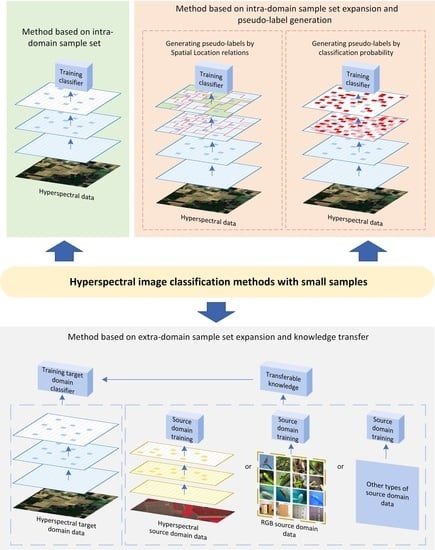
In this paper, we no longer use the learning paradigm as the taxonomy. Instead, the form of data utilization during model training is used as the classification basis of the model. Specifically, it can be divided into three categories (as shown in Figure 1).
- Method based on intra-domain sample set (IS): This method uses only the labeled samples in the current operation domain to train the model. Because of the limited amount of data available, these methods aim to extract as much useful information as possible from the available data. Approaches commonly used include developing better feature extraction techniques and enhancing the training set with more effective sample augmentation methods, among others.
- Method based on intra-domain sample set expansion and pseudo-label generation (ISE-PG): The most significant difference between this method and the first one is that it incorporates not only labeled data in the current operational domain but also partially unlabeled data in the same domain. Specifically, a portion of unlabeled data is selected from the current operational domain and pseudo-labels are generated for it, thereby enabling the expansion of the training sample size. The selection of samples from unlabeled regions in the current operational domain and the generation of pseudo-labels rely on labeled samples and prior knowledge.
- Method based on extra-domain sample set expansion and knowledge transfer (ESE-KT): This method is similar to the second method in that it also leverages data other than the labeled data in the current domain for auxiliary training. However, in this case, the data used for auxiliary training is not from the current operational domain, but from other domains. The representative works are various transfer learning methods including methods such as few shot learning. In applications, although there is less data available in the current domain, data from other domains may be more readily available. Therefore, finding the similarities between different domains and applying the transferable knowledge to model training in the current domain is also an important research direction.
We think the above taxonomy can be a good way to sort out the existing methods and provide a better indication of current research trends. Section 3 will provide a more comprehensive overview of representative methods in each category.
3. Methods
3.1. Methods Based on Intra-Domain Sample Set
Without the limitation of a small number of samples in the training set, past research on HSI classification has focused on how to improve the efficiency of data utilization during model training. Viewed from this perspective, optimizing feature engineering and classifier modules are fundamental to achieving high model performance. The IS-based approach is a continuation of this concept, which aims to improve the efficiency of data utilization in small sample settings [50,51].
As an extension of HSI classification method when the number of samples is sufficient, research on this type of method began earlier. For example, in [23], the authors generate a new feature set by feature space partitioning and kernel orthonormalized partial least square. In [52], the authors used affinity propagation-based band selection and conditional mutual information-based feature selection to generate a new feature representation for each labeled sample. Both methods classically start with a better feature representation. The original features are first mapped in a certain way and then the classifier is trained using the new feature set. In the era of non-deep learning, there are also articles that propose new methods from the perspective of optimizing classifiers. For example, ref. [21] uses rotation forest and adaboost, and ref. [19] uses a sparse representation classification method using homotopy. Regardless of the perspective, the aim of these methods is to extract more information from a limited sample.
With the rapid development of deep learning, numerous deep learning-based methods have been proposed for HIC-SS. The feature extractors and classifiers in deep models no longer have distinct boundaries but operate more as a whole. The proposal of multiple deep modules also provided more options to improve the efficiency of HSI utilization under small samples [53,54]. For example, ref. [24] is an early use of CNN for HIC-SS, demonstrating the feasibility of CNN even with a small amount of data. Many subsequent methods aimed to increase the performance of HIC-SS by improving the efficiency of limited training sample utilization using CNN-based methods. Zhang et al. proposed deep quadruplet network in [55], which is designed with a new quadruplet loss function to learn the feature space. Dong et al. proposed the pixel cluster theory in [56] to enrich the training set and exploit the advantages of CNN networks in feature extraction. Pal et al. proposed a new variance loss term to reduce network uncertainty and combined it with cross-entropy loss to train the model in an end-to-end manner [57]. Apart from proposing loss functions and data augmentation methods dedicated to this scenario, numerous network structure-level improvements have also proven effective. In recent years, the residual network module, attention module, and feature pyramid module, which have been widely used in other fields, have been introduced to HIC-SS to learn more useful information from a limited samples. For example, Ding et al. [58] proposed a hybrid model of 3D-CNN and 2D-CNN with a hybrid pyramidal feature fusion mechanism and a coordinated attention mechanism. Feng et al. [59] constructed a spatial feature cascade fusion network using two 3D spatial spectral residual modules and one 2D separable spatial residual module. This method constructs a cascade fusion model with intra-block feature fusion and inter-block feature fusion. In [60], Wu et al. proposed a two-channel CNN network for learning deep features of the training set to achieve higher accuracy classification. Additionally, the multiscale nested U-Net in [61] and the multidimensional CNN model with fused attention mechanism in [62] both make their own attempts at the model structure level.
In addition to the aforementioned models that aim to improve the connections between samples and classes, there is another category of models that focus on increasing the differentiability between classes (as depicted in Figure 2). The siamese network is a model that measures the similarity of two inputs. By setting an appropriate loss function, the siamese network can map samples into a feature space with improved separability, where the distance between similar samples is reduced and the distance between dissimilar samples is increased. Two siamese networks have been proposed for HIC-SS in [35] and [63], respectively. These networks use the original training set to create positive and negative sample pairs for siamese network training. The features mapped by the trained siamese network are then used to train the classification model. In addition to siamese networks, some authors have also proposed to learn the intrinsic relationship between labeled and unlabeled samples with the aid of graph information to alleviate the overfitting problem caused by fewer labeled samples [64].
IS-based methods aim to maximize the potential of available data by enhancing the efficiency of data utilization. This approach has been widely studied, and has a large existing literature. In some scenarios, satisfactory results have been achieved, and this method has provided valuable references for subsequent studies. However, the limitations of IS-based methods are evident. Since the entire information for building the model still essentially comes from a small number of labeled samples, the stability of the model suffers more when the training samples are poorly represented.
3.2. Method Based on Intra-Domain Sample Set Expansion and Pseudo-Label Generation
In contrast to the previous class of methods that prioritize data utilization efficiency, the ISE-PG-based method emphasizes the quantity of data. These methods aim to address the small-sample situation by increasing the number of available data. The selection of samples and the generation of labels are crucial factors in this class of methods.
For a classification model, both knowledge and data are directly related to performance. Knowledge refers to artificial experience that enables the model to differentiate between categories, such as the reflective properties of a certain target on a particular waveband or a certain association in the spatial distribution of targets. This knowledge can help the model label unlabeled samples under certain constraints and expand the training set. Moreover, knowledge is embedded in the data, and certain properties analyzed from specific samples may apply to the entire dataset. The ISE-PG based classification method is built on this foundation, and by introducing certain knowledge, the model can automatically select samples and assign labels. However, this process contains uncertainty, resulting in pseudo-labels with some degree of noise.
Spectral similarity serves as a foundation for sample selection and pseudo-label generation. As previously mentioned, HSI exhibit spectral mixing, causing some similar samples to present not exactly the same spectral curves. Nevertheless, samples with similar spectral curves still have a high probability of belonging to the same category in most cases. Hence, it is feasible to utilize spectral similarity as a criterion for pseudo-label generation. For instance, in [65], a hybrid label labeling model is proposed to label unlabeled data based on the existing training set using spectral similarity. Similarly, in another study [66], the authors assigned soft pseudo-labels by calculating the distance between unlabeled samples and labeled samples, which are also essentially based on the spectral similarity between samples.
In addition to spectral similarity, the spatial location relationship between samples can also be exploited to generate data pseudo-labels, as illustrated in Figure 3a. This is mainly related to the characteristics of HSI, where samples in a homogenous region are highly likely to belong to the same class label. Several studies have leveraged this theoretical basis, including Cui et al. who employed multiresolution segmentation to segment the HSI and then randomly selected unlabeled pixels in the same region as the labeled pixels and assigned them the same pseudo-label [67]. Similarly, Zheng et al. performed superpixel segmentation of the HSI and selected superpixels that contained only one labeled sample. The other unlabeled samples in this superpixel were then assigned the same pseudo-label as the labeled sample [68].
In addition to the aforementioned methods, some methods utilize both spectral similarity and spatial location relationships to determine the assignment of pseudo-labels. For example, in [69], the authors select unlabeled samples by calculating the spatial euclidean distance and spectral euclidean distance between samples. In another study, spectral angle distance is employed to enhance the accuracy of the generated pseudo-labels based on polygon segmentation results [70]. Similarly, the authors generated extended samples for labeled samples through superpixel segmentation maps and spectral nearest neighbor relationships in [71].
Methods that generate pseudo-labels by classification probabilities are also available, as illustrated in Figure 3b. These methods typically involve multiple training processes. In the previous iteration, the classifier is trained and then applied to the unlabeled data to make predictions. Pseudo-labels are assigned to some of the unlabeled data based on the prediction results. The pseudo-labeled data is then combined with the original data for the next training. Samples are continually selected and pseudo-labels generated during the multiple training runs until the stopping condition of the loop is satisfied [28,72,73].
The ISE-PG-based method has shown promise in addressing the issue of limited training samples by leveraging certain knowledge to select samples and generate pseudo-labels [68,70]. The incorporation of high-confidence pseudo-labels can mitigate the problem of class overlap and enhance the clarity of class boundaries. However, if the generated pseudo-labels are excessively noisy, they may negatively impact the training of the model. Furthermore, overconfident pseudo-labeling can also have a negative impact on the model’s performance. This is primarily due to the fact that such pseudo-labels may contain insufficient valid information, which could exacerbate the overfitting issue of the model.
3.3. Method Based on Extra-Domain Sample Set Expansion and Knowledge Transfer
In addition to the ISE-PG-based approach discussed above, there are also methods that address the HIC-SS problem by considering the data quantity perspective. This approach mainly takes into account the fact that in many cases there are limited data available in the current operational domain, but data from other domains are relatively easy to obtain. Thus, the challenge becomes how to utilize these other domains’ data for model training and apply the transferable knowledge learned to the current HSI processing, which is an interesting direction to explore [74,75,76].
Although this method emerged relatively recently, it has rapidly developed in recent years. Currently, these methods are mainly based on meta-learning theory, and their core mechanisms are roughly similar. Meta-learning is a form of implementation of few-shot learning and can also be considered a type of transfer learning [77,78,79]. Specifically, the focus of meta-learning is not on the model’s ability to perform a specific task, but on the model’s ability to learn how to learn [80,81,82]. In this sense, the meta-learning model is distinct from general machine learning models but is consistent with the way humans learn [83]. When faced with a new situation where they have never encountered the classes before, humans do not need a large number of new class samples to learn how to distinguish them [84,85]. Instead, they can quickly and accurately identify new classes based on just a few new class samples and previous learning experience [78]. This ability to build new models with only a few samples is generally lacking in current machine learning methods and is urgently needed in many application scenarios.
The meta-learning small sample classification method can be divided into three main stages: meta-learning on the source domain data, training on the target domain data, and testing on the target domain data (as illustrated in Figure 4). The source domain dataset contains a large number of data of different classes, which usually do not overlap with the classes in the target domain dataset. Meta-learning facilitates the acquisition of learning abilities by models during training, owing to its unique learning strategy. Unlike general machine learning algorithms, meta-learning’s basic training unit is the task. In meta-learning on the source domain data, the training process is called meta-training, and the testing process is called meta-testing. In the meta-training, the model is trained using a set of several different tasks. Each task has its own training set and test set. During the meta-training process, the model learns a generalized learning strategy by learning on these tasks so that it can quickly adapt to different tasks and data distributions. In the meta-testing, the model is tested using a new set of tasks that are different from the meta-training. These new tasks also have their own training and test sets, but do not overlap with the tasks in meta-training. In meta-testing, the model uses a generalized learning strategy previously learned in meta-training to quickly adapt and make predictions on the new tasks. Each task consisting of a support set and a query set. To simulate a small sample classification scenario, the classes included in the support set and query set are the same, but the number of samples per class in the support set is smaller than that in the query set. Additionally, the categories in the data are randomly selected from all categories in the dataset for each task. During the learning process, the support set’s samples are explicitly labeled, whereas the query set’s samples are considered to be unknown labeled. The algorithm parameters are updated by predicting the labels in the query set and calculating the losses. Following meta-training on the source domain data, a set of algorithm parameters F can be obtained, representing the transferable knowledge obtained by meta-learning. During target domain training, the algorithm parameters F obtained through meta-learning are involved in the training process along with the labeled data from the target domain, in order to obtain a model that can be used for classification in the target domain.
In terms of training process, most of these methods are metric-based meta-learning models. In simple terms, these models use meta-training to obtain a feature extraction module that embeds the input data into a deep metric space. Through feature embedding, samples that belong to the same class can be more aggregated, while samples of different classes are more dispersed. Since this module is obtained through meta-training, it can effectively complete feature embedding to improve sample separability even when the samples of new classes are small. A typical approach, such as deep few-shot learning (DFSL) [26], employs metric-based meta-learning to achieve feature embedding by using source domain data, and then uses k-nearest neighbor (KNN) or support vector machine (SVM) for classification. This approach has influenced subsequent studies, and many methods have similar designs [33,34,86,87,88]. In [89], the authors also proposed a metric-based meta-learning classification method based on adaptive subspaces and feature transformation. In addition to these methods mentioned above, there are some methods that are worthy of attention. For example, Gao et al. proposed the unsupervised meta-learning HIC-SS method [43]. Its unsupervised meta-learning task is constructed by generating multiple spatial spectral multi-view features for each unlabeled sample. Wang et al. explored the possibility of using heterogeneous data for meta-training and proposed the use of the RGB image dataset Mini-ImageNet for knowledge migration to help improve the accuracy of HIC-SS [90]. Other researchers have proposed using graph neural networks to construct metric-based meta-learning models [91,92], which have also achieved good classification results. Moreover, several other articles have proposed metric-based meta-learning HIC-SS methods [29,30,42,93].
In addition to the metric-based meta-learning methods discussed earlier, some articles also mention optimization-based meta-learning methods [94]. The core of the optimization-based meta-learning approach is to improve the optimization algorithm to enable the model to quickly adapt to new classification environments with only a small number of labeled samples. One notable example is the HIC-SS algorithm proposed by Gao et al. [37], which is built on a model-agnostic meta-learning mechanism.
The main idea behind the ESE-KT-based method is to transfer the knowledge obtained from source domain to the target domain, thereby addressing the challenge of target domain insufficient labeled data. Currently, this type of method is a key research direction in the field of HIC-SS and is considered as one of the most likely directions to achieve breakthroughs.
4. Performance
Taking SVM as the baseline [95], this section shows the performance of some HIC-SS methods proposed in recent years, and the covered methods are shown in Table 1. Due to inconsistent data and different number of training samples, direct comparison of the original results does not reflect the differences between the methods. In this paper, these methods are retrained and tested. To ensure the fairness and reliability of the experiments, all the results in this section are the mean of ten experimental results. Meanwhile, the training and testing sets used by all methods are the same for each run. In terms of evaluation indexes, we follow the most common metrics such as overall accuracy (OA), average accuracy (AA), and kappa coefficient to evaluate the performance of the methods comprehensively. Moreover, running time is also taken into account for a more comprehensive evaluation of the aforementioned methods.
4.1. Datasets
Experiments will be performed on three famous datasets and one new dataset, namely, Indian Pines (IP), Salinas Valley (SV), Pavia University (PU), and WHU-Hi-LongKou (LK). The False color image, ground truth and the number of each category for four datasets is shown in Table 2.
IP is collected by an airborne visible infrared imaging spectral sensor (AVIRIS) on the Purdue University agronomy farm and its surrounding land. The spatial resolution is 20 m, the spectral resolution is 10 nm, and the spectral range is 400–2500 nm, containing 224 bands, of which 200 are effective. Sixteen types are covered in the IP, including farmland, forest, and some buildings.
SV was collected by AVIRIS in Salinas Valley, California, USA. It has a spatial resolution of 3.7 m, a spectral resolution of 10 nm, and a spectral range of 400–2500 nm, and also contains 224 bands, of which 204 are effective bands. The SV has 16 classes of target, all of which are agricultural land types.
PU was acquired by the satellite-based ROSIS-03 sensor at the University of Pavia, Italy. The spatial resolution is 1.3 m, the spectral resolution is 4 nm, and the spectral range is 430–860 nm, containing 115 bands, of which 103 are effective. There are nine types of targets in PU, all of which are urban feature types.
LK was acquired by an 8 mm focal length Headwall Nano-Hyperspec imaging sensor on UAV platform in Longkou Town, Hubei province, China. The spatial resolution is 0.463 m. The spectral range is 400–1000 nm, containing 270 bands. This scene is a simple agricultural scene, which contains six crops and other three classes.
4.2. Sampling Strategy
Most current articles divide the original data into a training set and a test set by random sampling. In the first set of experiments, we followed this convention. Five samples from each category were randomly sampled separately as the training set, and all the remaining samples were used as the test set.
In addition to random sampling, we also adopt a disjointed sampling. While random sampling is commonly used in current HIC-SS research, it has certain limitations. Random sampling usually exposes some test samples to the model during the training, as illustrated in Figure 5 [98]. This will produce over-optimistic results on the test set [99], especially when dealing with small samples. This is because in the spatial information introduction, most existing methods deal with neighborhood slices centered on labeled samples. Additionally, random sampling is not practical in practical applications because training and test samples are often collected from different places. Therefore, it is essential to employ a more realistic disjointed sampling. Specifically, we randomly select one sample in each class and select the rest of the training samples in the neighborhood of that sample. As before, we use five samples for training and the remaining samples for testing purposes.
4.3. Performance Analysis
Table 3, Table 4, Table 5 and Table 6 present the classification results of the aforementioned methods for the four datasets under random sampling, with the corresponding classification maps displayed in Figure 6, Figure 7, Figure 8 and Figure 9. On the IP dataset, CTA achieved the best classification result with an OA and AA of more than 80%, which was the only method to achieve such a high performance. However, MFCN, PSG, and RN-FSC did not perform as well, with their OA not reaching 60%. When we compare the performance of IS, ISE-PG, and ESE-KT methods, it is observed that there are better and worse performing methods in each category. Overall, the ISE-PG-based methods such as CTA and STSE-DWLR performed slightly better on the IP dataset. We believe this is due to the lower spatial resolution of the IP data, which results in serious spectral mixing among samples. The spectral representations extracted from the limited training samples by most methods may not accurately describe the true characteristics of the classes. On the other hand, ISE-PG-based methods usually take the neighborhood relationship into account as an important basis for classification, and such an operation has been experimentally proven to be effective.
On the SV dataset, the classification results of the methods are more consistent, with fewer significant fluctuations compared to the previous set of experiments. Notably, the effectiveness of each method is significantly superior to that of SVM. In this set of experiments, DMVL, IHP-CA, CTA, and STSE-DWLR exhibit outstanding performance with an accuracy rate above 90% for each metric. CTA and STSE-DWLR exhibit remarkable stability on SV, achieving more than 95% classification accuracy. In addition, the four IS-based methods are generally better than the other four ESE-KT-based classification methods. This indicates that the classification methods using only intra-domain sample sets can also achieve better results when similar ground targets are more clustered.
On the PU dataset, the classification results of each method exhibit slight differences compared to the previous two sets of experiments. In this set of experiments, HFSL achieves the best classification results, not only exhibiting the highest average experimental outcomes in OA, AA, and Kappa coefficients, but also maintaining low variance in each metric, which reflects the remarkable stability of HFSL. Furthermore, IHP-CA, STSE-DWLR, and DCFSL demonstrate high classification performance. The excellent results of HFSL and DCFSL validate the significance of ESE-KT-based methods. When the samples exhibit a more dispersed distribution and the valid information contained in the neighborhood is insufficient, the transfer of knowledge from other datasets provides a positive reference for improving classification accuracy.
On the LK dataset, methods based on ISE-PG and ESE-KT achieve desirable results. CTA, STSE-DWLR, DCFSL, and HFSL all exhibit OA of over 90%, while RN-FSC and UM2L also demonstrate an OA of over 80%. However, the IS-based methods exhibit less satisfactory results. Furthermore, due to the category imbalance of the LK data, most of the algorithms showed significantly lower AA than OA, which was not seen in the previous three sets of experiments. Among the three metrics, HFSL demonstrates the most outstanding performance. The experimental results on the PU and LK datasets prove that HFSL is more appropriate for scenarios with higher spatial resolutions.
Overall, the ISE-PG method represented by CTA and STSE-DWLR demonstrated better classification results on data with lower spatial resolution under random sampling. This is mainly due to the fact that as the spatial resolution decreases, spectral mixing becomes more prominent and the reliability of the information extracted from a limited label sample decreases. In this case, pseudo-labeled samples with both correctness and representativeness can provide more valid information which can support model training. ESE-KT methods such as DCFSL and HFSL demonstrate more competitiveness when the resolution of the dataset is higher. When the spatial resolution is high, a small amount of labeled data can provide relatively consistent information. At this time, it is more difficult to continue to explore the potential of the target domain, which is a key factor limiting the performance of IS and ISE-PG methods. In this case, the advantage of ESE-KT is shown, and by seeking valid information from other domains, such methods bring the possibility for further improvement of model performance. In addition, IHP-CA belonging to IS is impressive in mining the available information in a small number of samples, demonstrating better classification performance on all four datasets. This also shows that the research on such methods is still of great importance in the current period.
Table 7, Table 8, Table 9 and Table 10 show the classification results of the above methods for the four datasets under the disjointed sampling (the classification map is shown in Figure 10, Figure 11, Figure 12 and Figure 13). As predicted in the previous section, in this case, the classification results of all methods show a significant decrease. Overall, it was found that some of the methods were less powerful than SVM on some dataset. Without exception, all of methods introduced spatial information in the model training, and all of them also achieved better results than the SVM using only spectral information when sampled randomly. It can be inferred that under the disjointed sampling, the effective mechanism of introducing spatial information in these methods will be greatly negatively affected.
In tests of IP data, most methods showed a 20–30% decline in classification accuracy compared to random sampling. The most effective CTA’s OA also showed a decline of about 25%. The classification accuracy of most methods was below 50%. It can be assumed that under this condition, the above methods basically lost the ability to identify targets in the IP dataset. In contrast, each method performs slightly better on SV data, with classification accuracy decreasing in the range of 10–20% basically. Among them, IHP-CA, CTA, and STSE-DWLR all achieved more than 80% classification accuracy and had more reliable recognition ability for most categories in SV. Compared with IP, SV data have high spatial resolution and less spectral mixing. Similar classes have more similar spectral curves in SV. In addition, the similar samples in SV data are also more clustered in terms of spatial distribution. These factors lead to a much lower impact on SV than on IP under disjointed sampling. The test results on the PU data also showed a similar situation to IP. All methods showed a significant drop in effectiveness, with five methods performing below the SVM. The overall accuracy of HFSL, which has the best classification result, also dropped sharply from 88.35% to 67.20%. On the LK dataset, most methods exhibit a decrease in classification accuracy of 10% to 30%. Similar to SV, similar samples are more clustered in LK, while possessing a higher spatial resolution. However, the negative impact of disjointed sampling on LK is evidently greater than that on SV. This is because there exist heterogeneous regions in certain categories of LK, as illustrated in the false color image of LK shown in Figure 2 (Some of the same categories appear as different colors on the false color image). These heterogenous regions exert a substantial impact on the performance of some methods under disjointed sampling. In addition, almost all methods showed greater variance in all three evaluation metrics and all four datasets under disjointed sampling. This indicates that the stability of each method is also affected more by the change of sampling method.
4.4. Performance with Different Numbers of Training Samples
In order to show the performance of the methods more comprehensively, we tested the classification results of all methods when the training samples were three to seven, respectively. The classification results with random sampling are shown in Figure 14. Under random sampling, most of the methods demonstrate a significant upward trend as the training sample size increases. On IP and SV, both CTA and STSE-DWLR maintain quite excellent classification performance under different training samples. On PU, HFSL has a clear advantage in classification performance. The situation demonstrated on LK is more complicated. When the training sample is three, the advantages of DCFSL, HFSL, and CTA are more obvious. However, when the training samples gradually increase, STSE-DWLR and RN-FSC also demonstrate excellent competitiveness. The results under random sampling are basically in line with our consistent intuition that an increase in the sample size brings more valid information, which improves the classification results.
The classification results under disjointed sampling are shown in Figure 15. Under disjointed sampling, as the training sample size is raised, all methods demonstrate a trend that is inconsistent with that under random sampling, and do not show a significant performance increase. This is because under disjointed sampling, the increased training samples are obtained in the neighborhood of the original samples, and their features are more similar to those of the original samples. Sample size increases of this magnitude bring limited additional information for model training. This also shows that under this sampling method, achieving accurate classification will face greater difficulties and has higher requirements for the design of the model.
4.5. Running Time
In addition to the classification accuracy, we also record the running times of all the above methods, as shown in Table 11. Combining the classification accuracy and running time, we can have a more comprehensive understanding of the performance of each method, so that we can choose a more suitable one for various application scenarios.
5. Perspectives
Achieving a model with outstanding performance while having a limited number of labeled samples is an arduous task, as the efficacy of the model is positively correlated with the number of training samples. Increasing the size of the training set is a direct approach to obtain satisfactory models in many fields. However, due to the characteristics of HSI, increasing the training set is often a challenging task. Hence, it is crucial to explore accurate classification methods for HSI that can perform well with a small number of samples.
In recent years, research on HIC-SS has been gradually increasing. From the current research, we believe that the following directions are full of potential for the future.
There is still a significant gap between the performance of existing methods and the actual demand, which makes it difficult to carry out practical applications. Although the recently proposed methods have been tried from different perspectives and achieved positive results, there is still considerable room for improvement.
In addition, it should be noted that most of the current research on HIC-SS is based on random sampling. However, this sampling strategy produces overly optimistic test results, and random sampling is not feasible in the reality that test samples and training samples are often from different regions. When using disjoint sampling, the performance of all methods decreases significantly, and some methods even lose the ability to identify targets completely. At present, there are few studies for HIC-SS built on disjoint sampling, and further research is needed.
In addition, transfer learning is currently being increasingly applied to solve HIC-SS, and has produced many promising results. However, there are still some key issues need to be further explored and demonstrated. On the one hand, the selection of source domains needs a basis. The existing methods involve not only HSI (including homogeneous HSI and heterogeneous HSI) but also other types of data (e.g., RGB images). The selection of source domains directly affects the effectiveness of knowledge transfer, so how to select the appropriate source domain for a specific target domain is a problem worth investigating. On the other hand, how to learn better transferable knowledge, or what kind of transferable knowledge is more effective for the target domain task, is also the focus of such methods.
In summary, despite the many advances in research on HIC-SS in recent years, there is still much work to be done. Achieving a more stable and accurate HIC-SS will remain a challenging task in the foreseeable future.
6. Conclusions
The lack of labeled samples is a major obstacle to achieve high-accuracy HSI classification. In most cases, manual labeling of HSI is time-consuming and costly; therefore, HIC-SS is a critical and urgent problem to be solved. In the past few years, HIC-SS has entered a period of rapid development, and a series of methods have been proposed. In this paper, we introduce a novel taxonomy and categorize some existing methods into three groups: IS-based methods, ISE-PG-based methods, and ESE-KT-based methods. Compared with the existing reviews, our proposed novel taxonomy is more conducive to the extraction and analysis of method generalities, thus making the categories more distinctive and distinguishable from each other. Furthermore, this paper conducts experiments on several recently proposed methods from each of the above three categories of methods under both random and disjointed sampling, visually demonstrating the advantages and limitations of relevant methods. Finally, we provide our perspectives on some current problems and possible future approaches of HIC-SS, which may have practical implications for future research. We believe that this paper is a good supplement to the existing review articles and helps readers to have a more comprehensive understanding of the current research status and future development trend of hyperspectral image classification with small samples.
Author Contributions
Conceptualization, X.W. and J.L.; data curation, X.W.; formal analysis, X.W.; funding acquisition, J.L.; investigation, X.W.; methodology, X.W.; project administration resources, J.L.; resources, J.L.; software, X.W. and W.C.; supervision, J.L. and W.W.; validation, X.W., W.C. and Y.N.; writing—original draft, X.W. and J.L.; writing—review and editing, X.W., J.L., W.C., W.W. and Y.N. All authors have read and agreed to the published version of the manuscript.
Funding
This work was supported in part by the Innovative talent program of Jiangsu under Grant JSSCR2021501, by Tianwen-2 Thermal Infrared Spectrometer for Asteroid Exploration granded by National Major Project, and by the High-level talent plan of NUAA, China.
Data Availability Statement
The Indiana Pines, Salinas Valley, and Pavia University datasets are available online at https://www.ehu.eus/ccwintco/index.php?title=Hyperspectral_Remote_Sensing_Scenes (accessed on 27 July 2023), and the WHU-Hi-LongKou dataset is available online at http://rsidea.whu.edu.cn/resource_WHUHi_sharing.htm (accessed on 27 July 2023).
Acknowledgments
All the authors thank Deren Li (Wuhan University) very much for his suggestions.
Conflicts of Interest
The authors declare no conflict of interest.
References
- Ghamisi, P.; Yokoya, N.; Li, J.; Liao, W.; Liu, S.; Plaza, J.; Rasti, B.; Plaza, A. Advances in Hyperspectral Image and Signal Processing: A Comprehensive Overview of the State of the Art. IEEE Geosci. Remote Sens. Mag. 2017, 5, 37–78. [Google Scholar] [CrossRef] [Green Version]
- Patro, R.N.; Subudhi, S.; Biswal, P.K.; Dell’acqua, F. A Review of Unsupervised Band Selection Techniques: Land Cover Classification for Hyperspectral Earth Observation Data. IEEE Geosci. Remote Sens. Mag. 2021, 9, 72–111. [Google Scholar] [CrossRef]
- Liang, L.; Di, L.; Zhang, L.; Deng, M.; Qin, Z.; Zhao, S.; Lin, H. Estimation of crop LAI using hyperspectral vegetation indices and a hybrid inversion method. Remote Sens. Environ. 2015, 165, 123–134. [Google Scholar] [CrossRef]
- Yang, X.; Yu, Y. Estimating Soil Salinity Under Various Moisture Conditions: An Experimental Study. IEEE Trans. Geosci. Remote Sens. 2017, 55, 2525–2533. [Google Scholar] [CrossRef]
- Yokoya, N.; Chan, J.C.W.; Segl, K. Potential of Resolution-Enhanced Hyperspectral Data for Mineral Mapping Using Simulated EnMAP and Sentinel-2 Images. Remote Sens. 2016, 8, 172. [Google Scholar] [CrossRef] [Green Version]
- Chang, C.I. Hyperspectral Data Exploitation: Theory and Applications; John Wiley and Sons: Hoboken, NJ, USA, 2007. [Google Scholar]
- Cao, X.; Wang, X.; Wang, D.; Zhao, J.; Jiao, L. Spectral–Spatial Hyperspectral Image Classification Using Cascaded Markov Random Fields. IEEE J. Sel. Top. Appl. Earth Obs. Remote Sens. 2019, 12, 4861–4872. [Google Scholar] [CrossRef]
- Cao, X.; Wang, D.; Wang, X.; Zhao, J.; Jiao, L. Hyperspectral imagery classification with cascaded support vector machines and multi-scale superpixel segmentation. Int. J. Remote Sens. 2020, 41, 4530–4550. [Google Scholar] [CrossRef]
- Ghamisi, P.; Maggiori, E.; Li, S.; Souza, R.; Tarablaka, Y.; Moser, G.; De Giorgi, A.; Fang, L.; Chen, Y.; Chi, M.; et al. New Frontiers in Spectral-Spatial Hyperspectral Image Classification: The Latest Advances Based on Mathematical Morphology, Markov Random Fields, Segmentation, Sparse Representation, and Deep Learning. IEEE Geosci. Remote Sens. Mag. 2018, 6, 10–43. [Google Scholar] [CrossRef]
- Bioucas-Dias, J.M.; Plaza, A.; Camps-Valls, G.; Scheunders, P.; Nasrabadi, N.; Chanussot, J. Hyperspectral Remote Sensing Data Analysis and Future Challenges. IEEE Geosci. Remote Sens. Mag. 2013, 1, 6–36. [Google Scholar] [CrossRef] [Green Version]
- Cubero-Castan, M.; Chanussot, J.; Achard, V.; Briottet, X.; Shimoni, M. A Physics-Based Unmixing Method to Estimate Subpixel Temperatures on Mixed Pixels. IEEE Trans. Geosci. Remote Sens. 2015, 53, 1894–1906. [Google Scholar] [CrossRef]
- Zhu, X.X.; Tuia, D.; Mou, L.; Xia, G.S.; Zhang, L.; Xu, F.; Fraundorfer, F. Deep Learning in Remote Sensing: A Comprehensive Review and List of Resources. IEEE Geosci. Remote Sens. Mag. 2017, 5, 8–36. [Google Scholar] [CrossRef] [Green Version]
- Paoletti, M.; Haut, J.; Plaza, J.; Plaza, A. Deep learning classifiers for hyperspectral imaging: A review. ISPRS J. Photogramm. Remote Sens. 2019, 158, 279–317. [Google Scholar] [CrossRef]
- Cen, Y.; Zhang, L.F.; Zhang, X.; Wang, Y.M.; Qi, W.C.; Tang, S.L.; Zhang, P. Aerial hyperspectral remote sensing classification dataset of Xiongan New Area (Matiwan Village). J. Remote Sens. 2020, 24, 1299–1306. [Google Scholar] [CrossRef]
- Yang, J.M.; Yu, P.T.; Kuo, B.C.; Huang, H.Y. A novel non-parametric weighted feature extraction method for classification of hyperspectral image with limited training samples. In Proceedings of the 2007 IEEE International Geoscience and Remote Sensing Symposium, Barcelona, Spain, 23–27 July 2007; pp. 1552–1555. [Google Scholar] [CrossRef]
- Prasad, S.; Bruce, L.M. Overcoming the Small Sample Size Problem in Hyperspectral Classification and Detection Tasks. In Proceedings of the IGARSS 2008—2008 IEEE International Geoscience and Remote Sensing Symposium, Boston, MA, USA, 6–11 July 2008; Volume 5, pp. V-381–V-384. [Google Scholar] [CrossRef]
- Imani, M.; Ghassemian, H. Feature Extraction Using Attraction Points for Classification of Hyperspectral Images in a Small Sample Size Situation. IEEE Geosci. Remote Sens. Lett. 2014, 11, 1986–1990. [Google Scholar] [CrossRef]
- Imani, M.; Ghassemian, H. Band Clustering-Based Feature Extraction for Classification of Hyperspectral Images Using Limited Training Samples. IEEE Geosci. Remote Sens. Lett. 2014, 11, 1325–1329. [Google Scholar] [CrossRef]
- Sami ul Haq, Q.; Tao, L.; Sun, F.; Yang, S. A Fast and Robust Sparse Approach for Hyperspectral Data Classification Using a Few Labeled Samples. IEEE Trans. Geosci. Remote Sens. 2012, 50, 2287–2302. [Google Scholar] [CrossRef]
- Li, F.; Xu, L.; Siva, P.; Wong, A.; Clausi, D.A. Hyperspectral Image Classification with Limited Labeled Training Samples Using Enhanced Ensemble Learning and Conditional Random Fields. IEEE J. Sel. Top. Appl. Earth Obs. Remote Sens. 2015, 8, 2427–2438. [Google Scholar] [CrossRef]
- Li, F.; Wong, A.; Clausi, D.A. Combining rotation forests and adaboost for hyperspectral imagery classification using few labeled samples. In Proceedings of the 2014 IEEE Geoscience and Remote Sensing Symposium, Quebec City, QC, Canada, 13–18 July 2014; pp. 4660–4663. [Google Scholar] [CrossRef]
- Xia, J.; Chanussot, J.; Du, P.; He, X. Rotation-Based Support Vector Machine Ensemble in Classification of Hyperspectral Data with Limited Training Samples. IEEE Trans. Geosci. Remote Sens. 2016, 54, 1519–1531. [Google Scholar] [CrossRef]
- Chen, J.; Xia, J.; Du, P.; Chanussot, J.; Xue, Z.; Xie, X. Kernel Supervised Ensemble Classifier for the Classification of Hyperspectral Data Using Few Labeled Samples. Remote Sens. 2016, 8, 601. [Google Scholar] [CrossRef] [Green Version]
- Yu, S.; Jia, S.; Xu, C. Convolutional neural networks for hyperspectral image classification. Neurocomputing 2017, 219, 88–98. [Google Scholar] [CrossRef]
- Pan, B.; Shi, Z.; Xu, X. MugNet: Deep learning for hyperspectral image classification using limited samples. ISPRS J. Photogramm. Remote Sens. 2018, 145, 108–119. [Google Scholar] [CrossRef]
- Liu, B.; Yu, X.; Yu, A.; Zhang, P.; Wan, G.; Wang, R. Deep Few-Shot Learning for Hyperspectral Image Classification. IEEE Trans. Geosci. Remote Sens. 2019, 57, 2290–2304. [Google Scholar] [CrossRef]
- Zhao, W.; Li, S.; Li, A.; Zhang, B.; Li, Y. Hyperspectral images classification with convolutional neural network and textural feature using limited training samples. Remote Sens. Lett. 2019, 10, 449–458. [Google Scholar] [CrossRef]
- Fang, B.; Li, Y.; Zhang, H.; Chan, J.C.W. Collaborative learning of lightweight convolutional neural network and deep clustering for hyperspectral image semi-supervised classification with limited training samples. ISPRS J. Photogramm. Remote Sens. 2020, 161, 164–178. [Google Scholar] [CrossRef]
- Gao, K.; Liu, B.; Yu, X.; Qin, J.; Zhang, P.; Tan, X. Deep Relation Network for Hyperspectral Image Few-Shot Classification. Remote Sens. 2020, 12, 923. [Google Scholar] [CrossRef] [Green Version]
- Gao, K.; Guo, W.; Yu, X.; Liu, B.; Yu, A.; Wei, X. Deep Induction Network for Small Samples Classification of Hyperspectral Images. IEEE J. Sel. Top. Appl. Earth Obs. Remote Sens. 2020, 13, 3462–3477. [Google Scholar] [CrossRef]
- Feng, Y.; Zheng, J.; Qin, M.; Bai, C.; Zhang, J. 3D Octave and 2D Vanilla Mixed Convolutional Neural Network for Hyperspectral Image Classification with Limited Samples. Remote Sens. 2021, 13, 4407. [Google Scholar] [CrossRef]
- Huang, L.; Chen, Y. Dual-Path Siamese CNN for Hyperspectral Image Classification with Limited Training Samples. IEEE Geosci. Remote Sens. Lett. 2021, 18, 518–522. [Google Scholar] [CrossRef]
- Li, Z.; Liu, M.; Chen, Y.; Xu, Y.; Li, W.; Du, Q. Deep Cross-Domain Few-Shot Learning for Hyperspectral Image Classification. IEEE Trans. Geosci. Remote Sens. 2022, 60, 1–18. [Google Scholar] [CrossRef]
- Bai, J.; Yuan, A.; Xiao, Z.; Zhou, H.; Wang, D.; Jiang, H.; Jiao, L. Class Incremental Learning with Few-Shots Based on Linear Programming for Hyperspectral Image Classification. IEEE Trans. Cybern. 2022, 52, 5474–5485. [Google Scholar] [CrossRef]
- Xue, Z.; Zhou, Y.; Du, P. S3Net: Spectral–Spatial Siamese Network for Few-Shot Hyperspectral Image Classification. IEEE Trans. Geosci. Remote Sens. 2022, 60, 1–19. [Google Scholar] [CrossRef]
- Liu, B.; Yu, X. Patch-Free Bilateral Network for Hyperspectral Image Classification Using Limited Samples. IEEE J. Sel. Top. Appl. Earth Obs. Remote Sens. 2021, 14, 10794–10807. [Google Scholar] [CrossRef]
- Gao, K.; Liu, B.; Yu, X.; Zhang, P.; Tan, X.; Sun, Y. Small sample classification of hyperspectral image using model-agnostic meta-learning algorithm and convolutional neural network. Int. J. Remote Sens. 2021, 42, 3090–3122. [Google Scholar] [CrossRef]
- Zhao, L.; Luo, W.; Liao, Q.; Chen, S.; Wu, J. Hyperspectral Image Classification with Contrastive Self-Supervised Learning Under Limited Labeled Samples. IEEE Geosci. Remote Sens. Lett. 2022, 19, 1–5. [Google Scholar] [CrossRef]
- Qu, Y.; Baghbaderani, R.K.; Qi, H. Few-Shot Hyperspectral Image Classification Through Multitask Transfer Learning. In Proceedings of the 2019 10th Workshop on Hyperspectral Imaging and Signal Processing: Evolution in Remote Sensing (WHISPERS), Amsterdam, The Netherlands, 24–26 September 2019; pp. 1–5. [Google Scholar] [CrossRef]
- Li, X.; Cao, Z.; Zhao, L.; Jiang, J. ALPN: Active-Learning-Based Prototypical Network for Few-Shot Hyperspectral Imagery Classification. IEEE Geosci. Remote Sens. Lett. 2022, 19, 1–5. [Google Scholar] [CrossRef]
- Thoreau, R.; Achard, V.; Risser, L.; Berthelot, B.; Briottet, X. Active Learning for Hyperspectral Image Classification: A comparative review. IEEE Geosci. Remote Sens. Mag. 2022, 10, 256–278. [Google Scholar] [CrossRef]
- Zhou, F.; Zhang, L.; Wei, W.; Bai, Z.; Zhang, Y. Meta Transfer Learning for Few-Shot Hyperspectral Image Classification. In Proceedings of the 2021 IEEE International Geoscience and Remote Sensing Symposium IGARSS, Brussels, Belgium, 11–16 July 2021; pp. 3681–3684. [Google Scholar] [CrossRef]
- Gao, K.; Liu, B.; Yu, X.; Yu, A. Unsupervised Meta Learning with Multiview Constraints for Hyperspectral Image Small Sample set Classification. IEEE Trans. Image Process. 2022, 31, 3449–3462. [Google Scholar] [CrossRef]
- Jia, S.; Jiang, S.; Lin, Z.; Li, N.; Xu, M.; Yu, S. A survey: Deep learning for hyperspectral image classification with few labeled samples. Neurocomputing 2021, 448, 179–204. [Google Scholar] [CrossRef]
- Li, X.; Li, Z.; Qiu, H.; Hou, G.; Fan, P. An overview of hyperspectral image feature extraction, classification methods and the methods based on small samples. Appl. Spectrosc. Rev. 2021, 58, 367–400. [Google Scholar] [CrossRef]
- Wambugu, N.; Chen, Y.; Xiao, Z.; Tan, K.; Wei, M.; Liu, X.; Li, J. Hyperspectral image classification on insufficient-sample and feature learning using deep neural networks: A review. Int. J. Appl. Earth Obs. Geoinf. 2021, 105, 102603. [Google Scholar] [CrossRef]
- Doersch, C.; Gupta, A.; Zisserman, A. CrossTransformers: Spatially-aware few-shot transfer. In Proceedings of the Advances in Neural Information Processing Systems; Larochelle, H., Ranzato, M., Hadsell, R., Balcan, M., Lin, H., Eds.; Curran Associates, Inc.: New York, NY, USA, 2020; Volume 33, pp. 21981–21993. [Google Scholar]
- Luo, X.; Wei, L.; Wen, L.; Yang, J.; Xie, L.; Xu, Z.; Tian, Q. Rectifying the shortcut learning of background for few-shot learning. Adv. Neural Inf. Process. Syst. 2021, 34, 13073–13085. [Google Scholar]
- Luo, X.; Xu, J.; Xu, Z. Channel importance matters in few-shot image classification. In Proceedings of the International Conference on Machine Learning, Baltimore, MA, USA, 17–23 July 2022; pp. 14542–14559. [Google Scholar]
- Karaca, A.C. Spatial aware probabilistic multi-kernel collaborative representation for hyperspectral image classification using few labelled samples. Int. J. Remote Sens. 2021, 42, 839–864. [Google Scholar] [CrossRef]
- Karaca, A.C. Domain Transform Filter and Spatial-Aware Collaborative Representation for Hyperspectral Image Classification Using Few Labeled Samples. IEEE Geosci. Remote Sens. Lett. 2021, 18, 1264–1268. [Google Scholar] [CrossRef]
- Jia, S.; Zhu, Z.; Shen, L.; Li, Q. A Two-Stage Feature Selection Framework for Hyperspectral Image Classification Using Few Labeled Samples. IEEE J. Sel. Top. Appl. Earth Obs. Remote Sens. 2014, 7, 1023–1035. [Google Scholar] [CrossRef]
- Wang, A.; Liu, C.; Xue, D.; Wu, H.; Zhang, Y.; Liu, M. Depthwise Separable Relation Network for Small Sample Hyperspectral Image Classification. Symmetry 2021, 13, 1673. [Google Scholar] [CrossRef]
- Pan, H.; Liu, M.; Ge, H.; Wang, L. One-Shot Dense Network with Polarized Attention for Hyperspectral Image Classification. Remote Sens. 2022, 14, 2265. [Google Scholar] [CrossRef]
- Zhang, C.; Yue, J.; Qin, Q. Deep Quadruplet Network for Hyperspectral Image Classification with a Small Number of Samples. Remote Sens. 2020, 12, 647. [Google Scholar] [CrossRef] [Green Version]
- Dong, S.; Quan, Y.; Feng, W.; Dauphin, G.; Gao, L.; Xing, M. A Pixel Cluster CNN and Spectral-Spatial Fusion Algorithm for Hyperspectral Image Classification with Small-Size Training Samples. IEEE J. Sel. Top. Appl. Earth Obs. Remote Sens. 2021, 14, 4101–4114. [Google Scholar] [CrossRef]
- Pal, D.; Bundele, V.; Banerjee, B.; Jeppu, Y. SPN: Stable Prototypical Network for Few-Shot Learning-Based Hyperspectral Image Classification. IEEE Geosci. Remote Sens. Lett. 2022, 19, 1–5. [Google Scholar] [CrossRef]
- Ding, C.; Chen, Y.; Li, R.; Wen, D.; Xie, X.; Zhang, L.; Wei, W.; Zhang, Y. Integrating Hybrid Pyramid Feature Fusion and Coordinate Attention for Effective Small Sample Hyperspectral Image Classification. Remote Sens. 2022, 14, 2355. [Google Scholar] [CrossRef]
- Feng, F.; Zhang, Y.; Zhang, J.; Liu, B. Small Sample Hyperspectral Image Classification Based on Cascade Fusion of Mixed Spatial-Spectral Features and Second-Order Pooling. Remote Sens. 2022, 14, 505. [Google Scholar] [CrossRef]
- Wu, H.; Wang, L.; Shi, Y. Convolution neural network method for small-sample classification of hyperspectral images. J. Image Graph. 2021, 26, 2009–2020. [Google Scholar]
- Liu, B.; Yu, A.; Gao, K.; Wang, Y.; Yu, X.; Zhang, P. Multiscale nested U-Net for small sample classification of hyperspectral images. J. Appl. Remote Sens. 2022, 16, 016506. [Google Scholar] [CrossRef]
- Liu, J.; Zhang, K.; Wu, S.; Shi, H.; Zhao, Y.; Sun, Y.; Zhuang, H.; Fu, E. An Investigation of a Multidimensional CNN Combined with an Attention Mechanism Model to Resolve Small-Sample Problems in Hyperspectral Image Classification. Remote Sens. 2022, 14, 785. [Google Scholar] [CrossRef]
- Cao, Z.; Li, X.; Jiang, J.; Zhao, L. 3D convolutional siamese network for few-shot hyperspectral classification. J. Appl. Remote Sens. 2020, 14, 048504. [Google Scholar] [CrossRef]
- Li, N.; Zhou, D.; Shi, J.; Zheng, X.; Wu, T.; Yang, Z. Graph-Based Deep Multitask Few-Shot Learning for Hyperspectral Image Classification. Remote Sens. 2022, 14, 2246. [Google Scholar] [CrossRef]
- Wei, W.; Zhang, L.; Li, Y.; Wang, C.; Zhang, Y. Intraclass Similarity Structure Representation-Based Hyperspectral Imagery Classification with Few Samples. IEEE J. Sel. Top. Appl. Earth Obs. Remote Sens. 2020, 13, 1045–1054. [Google Scholar] [CrossRef]
- Ding, C.; Li, Y.; Wen, Y.; Zheng, M.; Zhang, L.; Wei, W.; Zhang, Y. Boosting Few-Shot Hyperspectral Image Classification Using Pseudo-Label Learning. Remote Sens. 2021, 13, 3539. [Google Scholar] [CrossRef]
- Cui, B.; Ma, X.; Zhao, F.; Wu, Y. A novel hyperspectral image classification approach based on multiresolution segmentation with a few labeled samples. Int. J. Adv. Robot. Syst. 2017, 14, 1729881417710219. [Google Scholar] [CrossRef]
- Zheng, C.; Wang, N.; Cui, J. Hyperspectral Image Classification with Small Training Sample Size Using Superpixel-Guided Training Sample Enlargement. IEEE Trans. Geosci. Remote Sens. 2019, 57, 7307–7316. [Google Scholar] [CrossRef]
- Romaszewski, M.; Głomb, P.; Cholewa, M. Semi-supervised hyperspectral classification from a small number of training samples using a co-training approach. ISPRS J. Photogramm. Remote Sens. 2016, 121, 60–76. [Google Scholar] [CrossRef]
- Zhang, S.; Kang, X.; Duan, P.; Sun, B.; Li, S. Polygon Structure-Guided Hyperspectral Image Classification with Single Sample for Strong Geometric Characteristics Scenes. IEEE Trans. Geosci. Remote Sens. 2022, 60, 1–12. [Google Scholar] [CrossRef]
- Hu, X.; Si, H. Hyperspectral Image Classification Method with Small Sample Set Based on Adaptive Dictionary. Trans. Chin. Soc. Agric. Mach. 2021, 52, 154–161. [Google Scholar]
- Feng, W.; Huang, W.; Dauphin, G.; Xia, J.; Quan, Y.; Ye, H.; Dong, Y. Ensemble Margin Based Semi-Supervised Random Forest for the Classification of Hyperspectral Image with Limited Training Data. In Proceedings of the IGARSS 2019—2019 IEEE International Geoscience and Remote Sensing Symposium, Yokohama, Japan, 28 July–2 August 2019; pp. 971–974. [Google Scholar] [CrossRef]
- Feng, W.; Quan, Y.; Dauphin, G.; Li, Q.; Gao, L.; Huang, W.; Xia, J.; Zhu, W.; Xing, M. Semi-supervised rotation forest based on ensemble margin theory for the classification of hyperspectral image with limited training data. Inf. Sci. 2021, 575, 611–638. [Google Scholar] [CrossRef]
- Yang, J.; Zhao, Y.Q.; Chan, J.C.W. Learning and Transferring Deep Joint Spectral–Spatial Features for Hyperspectral Classification. IEEE Trans. Geosci. Remote Sens. 2017, 55, 4729–4742. [Google Scholar] [CrossRef]
- Liang, H.; Fu, W.; Yi, F. A survey of recent advances in transfer learning. In Proceedings of the 2019 IEEE 19th international conference on communication technology (ICCT), Xi’an, China, 16–19 October 2019; pp. 1516–1523. [Google Scholar]
- Liu, B.; Yu, X.; Yu, A.; Wan, G. Deep convolutional recurrent neural network with transfer learning for hyperspectral image classification. J. Appl. Remote Sens. 2018, 12, 026028. [Google Scholar] [CrossRef]
- Sung, F.; Yang, Y.; Zhang, L.; Xiang, T.; Torr, P.H.; Hospedales, T.M. Learning to Compare: Relation Network for Few-Shot Learning. In Proceedings of the 2018 IEEE/CVF Conference on Computer Vision and Pattern Recognition, Salt Lake City, UT, USA, 18–23 June 2018; pp. 1199–1208. [Google Scholar] [CrossRef] [Green Version]
- Vinyals, O.; Blundell, C.; Lillicrap, T.; Kavukcuoglu, K.; Wierstra, D. Matching networks for one shot learning. Adv. Neural Inf. Process. Syst. 2016, 29, 3637–3645. [Google Scholar]
- Snell, J.; Swersky, K.; Zemel, R. Prototypical networks for few-shot learning. Adv. Neural Inf. Process. Syst. 2017, 30, 4080–4090. [Google Scholar]
- Chen, W.Y.; Liu, Y.C.; Kira, Z.; Wang, Y.C.F.; Huang, J.B. A closer look at few-shot classification. arXiv 2019, arXiv:1904.04232. [Google Scholar]
- Ren, M.; Triantafillou, E.; Ravi, S.; Snell, J.; Swersky, K.; Tenenbaum, J.B.; Larochelle, H.; Zemel, R.S. Meta-learning for semi-supervised few-shot classification. arXiv 2018, arXiv:1803.00676. [Google Scholar]
- Andrychowicz, M.; Denil, M.; Gomez, S.; Hoffman, M.W.; Pfau, D.; Schaul, T.; Shillingford, B.; De Freitas, N. Learning to learn by gradient descent by gradient descent. Adv. Neural Inf. Process. Syst. 2016, 29, 3988–3996. [Google Scholar]
- Li, Z.; Zhou, F.; Chen, F.; Li, H. Meta-sgd: Learning to learn quickly for few-shot learning. arXiv 2017, arXiv:1707.09835. [Google Scholar]
- Wang, Y.; Yao, Q.; Kwok, J.T.; Ni, L.M. Generalizing from a few examples: A survey on few-shot learning. ACM Comput. Surv. 2020, 53, 1–34. [Google Scholar] [CrossRef]
- Ravi, S.; Larochelle, H. Optimization as a model for few-shot learning. In Proceedings of the International Conference on Learning Representations, San Juan, Puerto Rico, 2–4 May 2016. [Google Scholar]
- Liu, B.; Zuo, X.; Tan, X.; Yu, A.; Guo, W. A Deep few-shot learning algorithm for hyperspectral image classification. Acta Geod. Cartogr. Sin. 2020, 49, 1331–1342. [Google Scholar]
- Zhang, C.; Yue, J.; Qin, Q. Global Prototypical Network for Few-Shot Hyperspectral Image Classification. IEEE J. Sel. Top. Appl. Earth Obs. Remote Sens. 2020, 13, 4748–4759. [Google Scholar] [CrossRef]
- Liang, X.; Zhang, Y.; Zhang, J. Attention Multisource Fusion-Based Deep Few-Shot Learning for Hyperspectral Image Classification. IEEE J. Sel. Top. Appl. Earth Obs. Remote Sens. 2021, 14, 8773–8788. [Google Scholar] [CrossRef]
- Bai, J.; Huang, S.; Xiao, Z.; Li, X.; Zhu, Y.; Regan, A.C.; Jiao, L. Few-Shot Hyperspectral Image Classification Based on Adaptive Subspaces and Feature Transformation. IEEE Trans. Geosci. Remote Sens. 2022, 60, 1–17. [Google Scholar] [CrossRef]
- Wang, Y.; Liu, M.; Yang, Y.; Li, Z.; Du, Q.; Chen, Y.; Li, F.; Yang, H. Heterogeneous Few-Shot Learning for Hyperspectral Image Classification. IEEE Geosci. Remote Sens. Lett. 2022, 19, 1–5. [Google Scholar] [CrossRef]
- Zuo, X.; Yu, X.; Liu, B.; Zhang, P.; Tan, X. FSL-EGNN: Edge-Labeling Graph Neural Network for Hyperspectral Image Few-Shot Classification. IEEE Trans. Geosci. Remote Sens. 2022, 60, 1–18. [Google Scholar] [CrossRef]
- Xinyi, T.; Jihao, Y.; Bingnan, H.; Hui, Q. Few-Shot Learning with Attention-Weighted Graph Convolutional Networks For Hyperspectral Image Classification. In Proceedings of the 2020 IEEE International Conference on Image Processing (ICIP), Abu Dhabi, United Arab Emirates, 25–28 October 2020; pp. 1686–1690. [Google Scholar] [CrossRef]
- Huang, K.; Deng, X.; Geng, J.; Jiang, W. Self-Attention and Mutual-Attention for Few-Shot Hyperspectral Image Classification. In Proceedings of the 2021 IEEE International Geoscience and Remote Sensing Symposium IGARSS, Brussels, Belgium, 11–16 July 2021; pp. 2230–2233. [Google Scholar] [CrossRef]
- Finn, C.; Abbeel, P.; Levine, S. Model-agnostic meta-learning for fast adaptation of deep networks. In Proceedings of the International Conference on Machine Learning, Sydney, Australia, 6–11 August 2017; pp. 1126–1135. [Google Scholar]
- Melgani, F.; Bruzzone, L. Support vector machines for classification of hyperspectral remote-sensing images. In Proceedings of the IEEE International Geoscience and Remote Sensing Symposium, Toronto, ON, Canada, 24–28 June 2002; Volume 1, pp. 506–508. [Google Scholar] [CrossRef]
- Liu, B.; Yu, A.; Yu, X.; Wang, R.; Gao, K.; Guo, W. Deep Multiview Learning for Hyperspectral Image Classification. IEEE Trans. Geosci. Remote Sens. 2021, 59, 7758–7772. [Google Scholar] [CrossRef]
- Xu, B.; Hou, W.; Wei, Y.; Wang, Y.; Li, X. Minimalistic fully convolution networks (MFCN): Pixel-level classification for hyperspectral image with few labeled samples. Opt. Express 2022, 30, 16585–16605. [Google Scholar] [CrossRef] [PubMed]
- Audebert, N.; Le Saux, B.; Lefevre, S. Deep Learning for Classification of Hyperspectral Data: A Comparative Review. IEEE Geosci. Remote Sens. Mag. 2019, 7, 159–173. [Google Scholar] [CrossRef] [Green Version]
- Cao, X.; Liu, Z.; Li, X.; Xiao, Q.; Feng, J.; Jiao, L. Nonoverlapped Sampling for Hyperspectral Imagery: Performance Evaluation and a Cotraining-Based Classification Strategy. IEEE Trans. Geosci. Remote Sens. 2022, 60, 1–14. [Google Scholar] [CrossRef]
Figure 1.
Schematic diagram of the training process of the three types of methods; the dark blue squares represent the original training samples. (a) Method based on intra-domain sample set: The classifier is trained on the original training samples of the current data. (b) Method based on intra-domain sample set expansion and pseudo-label generation: The green squares represents the pseudo-labeled intra-domain extension samples, and the classifier is trained on the original samples and the intra-domain extension samples. (c) Method based on extra-domain sample set expansion and knowledge transfer: The dashed box on the left represents intra-domain data and the dashed box on the right represents extra-domain data. The dark yellow squares represent samples from other hyperspectral datasets. By training on hyperspectral source domain data or other types of source domain data, the learned transferable knowledge is then used to help train the target domain classifier.

Figure 2.
Two typical IS-based models. The top right model focuses on how to build a stronger relationship between samples and classes (different shapes represent classification boundaries for different classes). The lower right model focuses on how to increase the differentiability between different classes (the hollow circles in the figure represent a class as a whole).

Figure 3.
The current commonly used pseudo-label generation mechanisms. (a) Generating pseudo-labels by spatial location relations. The blue squares are the original training set. The red line indicates the segmentation result. The green squares are the extended data with pseudo-labels. The pseudo-labels are generated by combining the spatial segmentation results of the images and the original training set. (b) Generating pseudo-labels by classification probability. The blue squares are the original training set. The different red colors represent the confidence of the test samples’ results in the previous classification; the darker the color, the higher the confidence. The extended samples consist of samples with high confidence whose pseudo-labels are the predicted labels of the previous classification.

Figure 4.
Schematic diagram of the meta-learning based methods, where different colors represent different classes. First, meta-learning is performed on the source domain data. Meta-learning is divided into meta-training and meta-testing. Both meta-training and meta-testing are task-based, and each task contains the process of complete training and testing of certain categories. Thus, each task corresponds to a classification model f. F can be obtained by performing meta-learning on these tasks, which contains transferable knowledge (e.g., locally optimal algorithm parameters) for the current scene. After completing the meta-learning in the source domain, F is applied to the training of the classification model in the target domain, and the final classification model is obtained.

Figure 5.
(a) Random sampling and (b) disjointed sampling. Each square in the image represents a sample: dark blue represents the test sample, light blue represents the training sample, dark green represents the test sample in the neighborhood of the training sample (gray points as an example), and light green represents the other training samples in the neighborhood of the training sample. If the spatial information of a training sample is extracted in a 3 × 3 neighborhood, the neighborhood under random sampling will contain more test samples, which will lead to artificially high accuracy when testing.

Figure 6.
Classification maps of IP dataset under random sampling. (a) SVM. (b) DMVL. (c) IHP-CA. (d) MFCN. (e) S3Net. (f) CTA. (g) STSE-DWLR. (h) PSG. (i) RN-FSC. (j) UM2L. (k) DCFSL. (l) HFSL.
Figure 6.
Classification maps of IP dataset under random sampling. (a) SVM. (b) DMVL. (c) IHP-CA. (d) MFCN. (e) S3Net. (f) CTA. (g) STSE-DWLR. (h) PSG. (i) RN-FSC. (j) UM2L. (k) DCFSL. (l) HFSL.

Figure 7.
Classification maps of SV dataset under random sampling. (a) SVM. (b) DMVL. (c) IHP-CA. (d) MFCN. (e) S3Net. (f) CTA. (g) STSE-DWLR. (h) PSG. (i) RN-FSC. (j) UM2L. (k) DCFSL. (l) HFSL.
Figure 7.
Classification maps of SV dataset under random sampling. (a) SVM. (b) DMVL. (c) IHP-CA. (d) MFCN. (e) S3Net. (f) CTA. (g) STSE-DWLR. (h) PSG. (i) RN-FSC. (j) UM2L. (k) DCFSL. (l) HFSL.

Figure 8.
Classification maps of PU dataset under random sampling. (a) SVM. (b) DMVL. (c) IHP-CA. (d) MFCN. (e) S3Net. (f) CTA. (g) STSE-DWLR. (h) PSG. (i) RN-FSC. (j) UM2L. (k) DCFSL. (l) HFSL.
Figure 8.
Classification maps of PU dataset under random sampling. (a) SVM. (b) DMVL. (c) IHP-CA. (d) MFCN. (e) S3Net. (f) CTA. (g) STSE-DWLR. (h) PSG. (i) RN-FSC. (j) UM2L. (k) DCFSL. (l) HFSL.

Figure 9.
Classification maps of LK dataset under random sampling. (a) SVM. (b) DMVL. (c) IHP-CA. (d) MFCN. (e) S3Net. (f) CTA. (g) STSE-DWLR. (h) PSG. (i) RN-FSC. (j) UM2L. (k) DCFSL. (l) HFSL.
Figure 9.
Classification maps of LK dataset under random sampling. (a) SVM. (b) DMVL. (c) IHP-CA. (d) MFCN. (e) S3Net. (f) CTA. (g) STSE-DWLR. (h) PSG. (i) RN-FSC. (j) UM2L. (k) DCFSL. (l) HFSL.

Figure 10.
Classification maps of IP dataset under disjointed sampling. (a) SVM. (b) DMVL. (c) IHP-CA. (d) MFCN. (e) S3Net. (f) CTA. (g) STSE-DWLR. (h) PSG. (i) RN-FSC. (j) UM2L. (k) DCFSL. (l) HFSL.
Figure 10.
Classification maps of IP dataset under disjointed sampling. (a) SVM. (b) DMVL. (c) IHP-CA. (d) MFCN. (e) S3Net. (f) CTA. (g) STSE-DWLR. (h) PSG. (i) RN-FSC. (j) UM2L. (k) DCFSL. (l) HFSL.

Figure 11.
Classification maps of SV dataset under disjointed sampling. (a) SVM. (b) DMVL. (c) IHP-CA. (d) MFCN. (e) S3Net. (f) CTA. (g) STSE-DWLR. (h) PSG. (i) RN-FSC. (j) UM2L. (k) DCFSL. (l) HFSL.
Figure 11.
Classification maps of SV dataset under disjointed sampling. (a) SVM. (b) DMVL. (c) IHP-CA. (d) MFCN. (e) S3Net. (f) CTA. (g) STSE-DWLR. (h) PSG. (i) RN-FSC. (j) UM2L. (k) DCFSL. (l) HFSL.

Figure 12.
Classification maps of PU dataset under disjointed sampling. (a) SVM. (b) DMVL. (c) IHP-CA. (d) MFCN. (e) S3Net. (f) CTA. (g) STSE-DWLR. (h) PSG. (i) RN-FSC. (j) UM2L. (k) DCFSL. (l) HFSL.
Figure 12.
Classification maps of PU dataset under disjointed sampling. (a) SVM. (b) DMVL. (c) IHP-CA. (d) MFCN. (e) S3Net. (f) CTA. (g) STSE-DWLR. (h) PSG. (i) RN-FSC. (j) UM2L. (k) DCFSL. (l) HFSL.

Figure 13.
Classification maps of LK dataset under disjointed sampling. (a) SVM. (b) DMVL. (c) IHP-CA. (d) MFCN. (e) S3Net. (f) CTA. (g) STSE-DWLR. (h) PSG. (i) RN-FSC. (j) UM2L. (k) DCFSL. (l) HFSL.
Figure 13.
Classification maps of LK dataset under disjointed sampling. (a) SVM. (b) DMVL. (c) IHP-CA. (d) MFCN. (e) S3Net. (f) CTA. (g) STSE-DWLR. (h) PSG. (i) RN-FSC. (j) UM2L. (k) DCFSL. (l) HFSL.

Figure 14.
Overall accuracy with different training sample sizes under random sampling. (a) IP. (b) SV. (c) PU. (d) LK.
Figure 14.
Overall accuracy with different training sample sizes under random sampling. (a) IP. (b) SV. (c) PU. (d) LK.

Figure 15.
Overall accuracy with different training sample sizes under disjointed sampling. (a) IP. (b) SV. (c) PU. (d) LK.
Figure 15.
Overall accuracy with different training sample sizes under disjointed sampling. (a) IP. (b) SV. (c) PU. (d) LK.


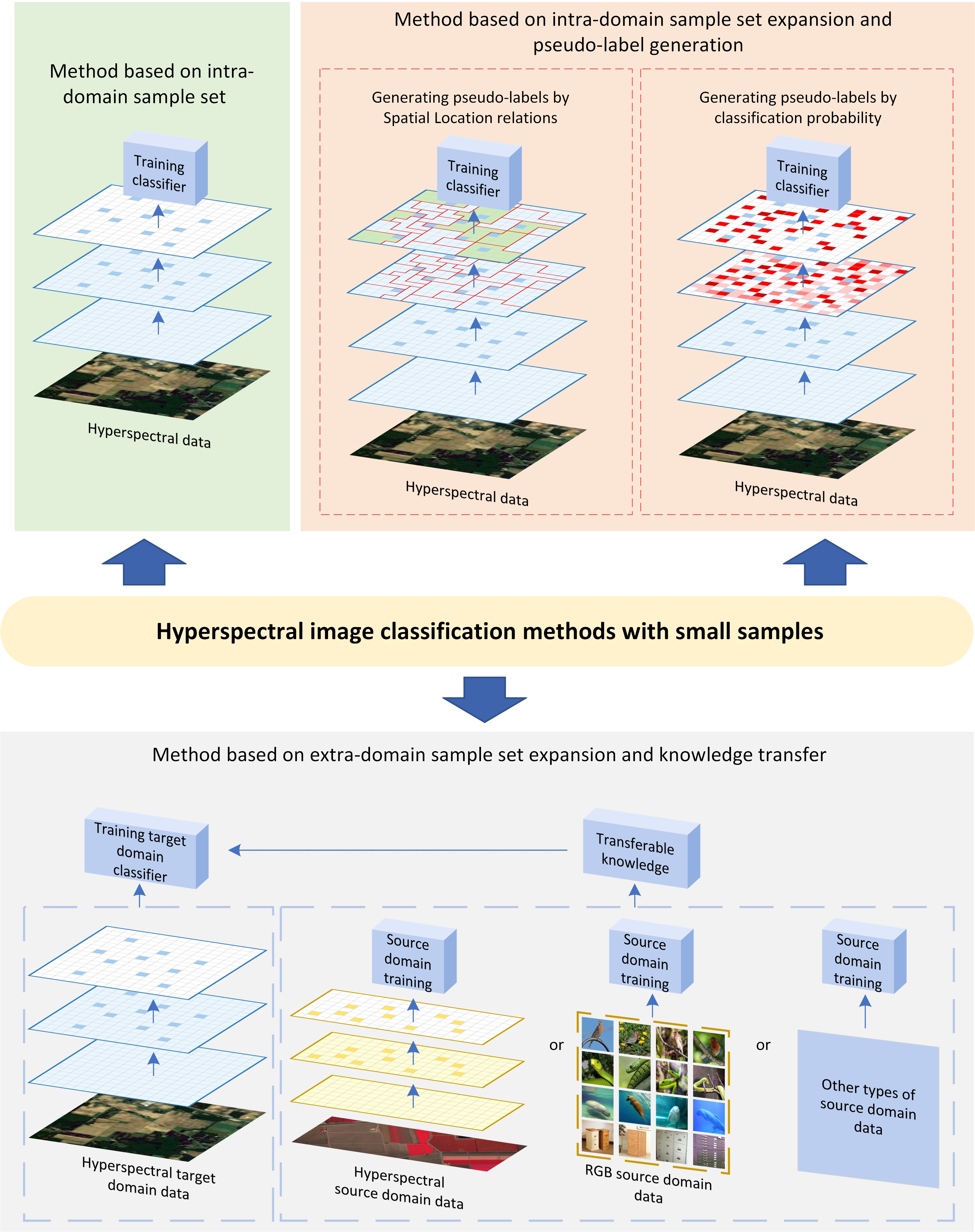
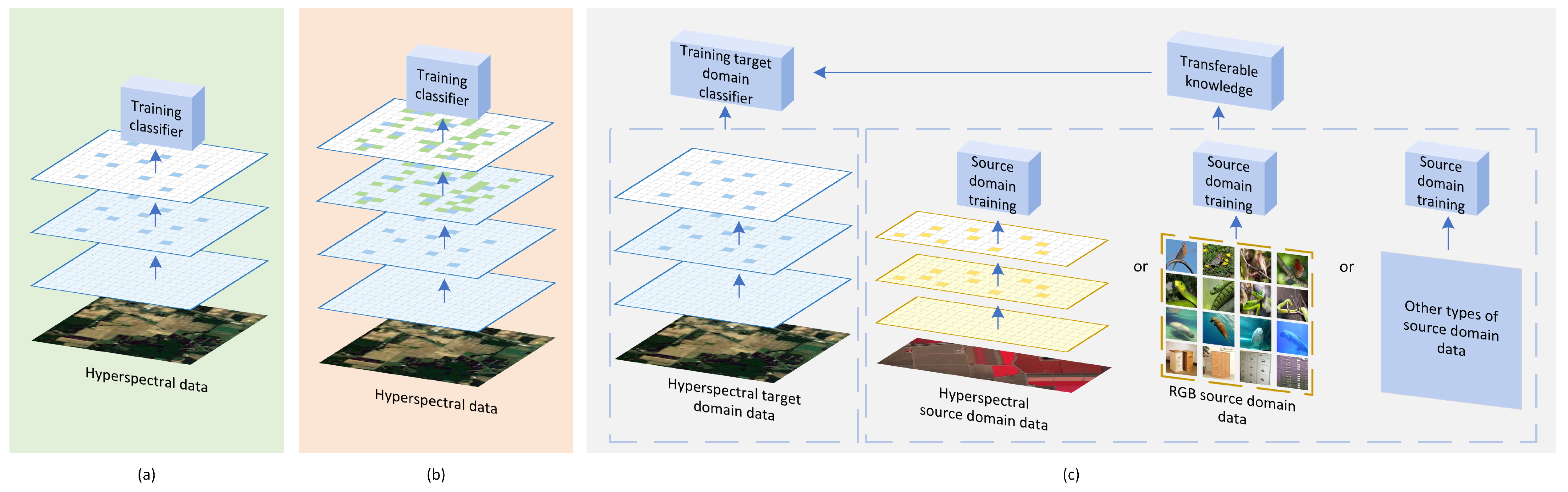
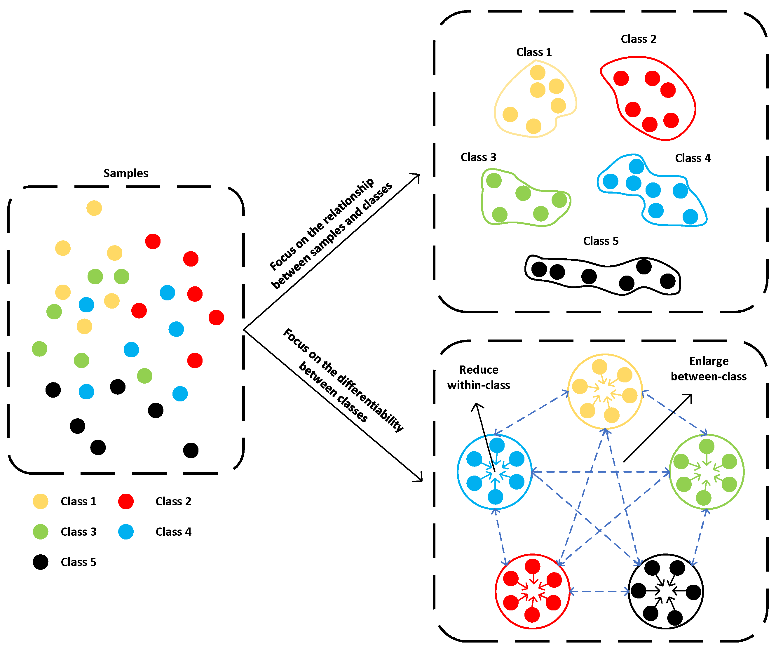
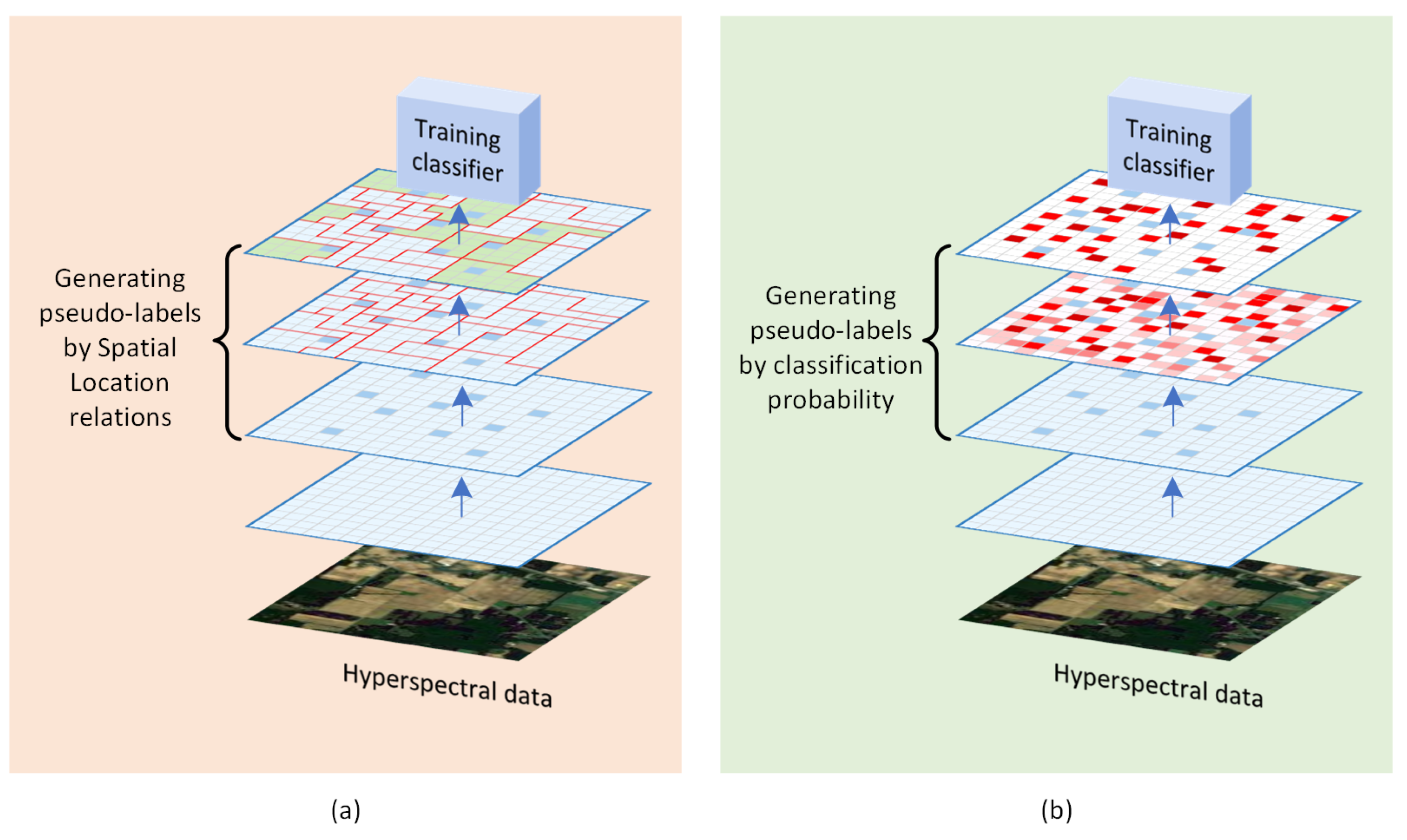
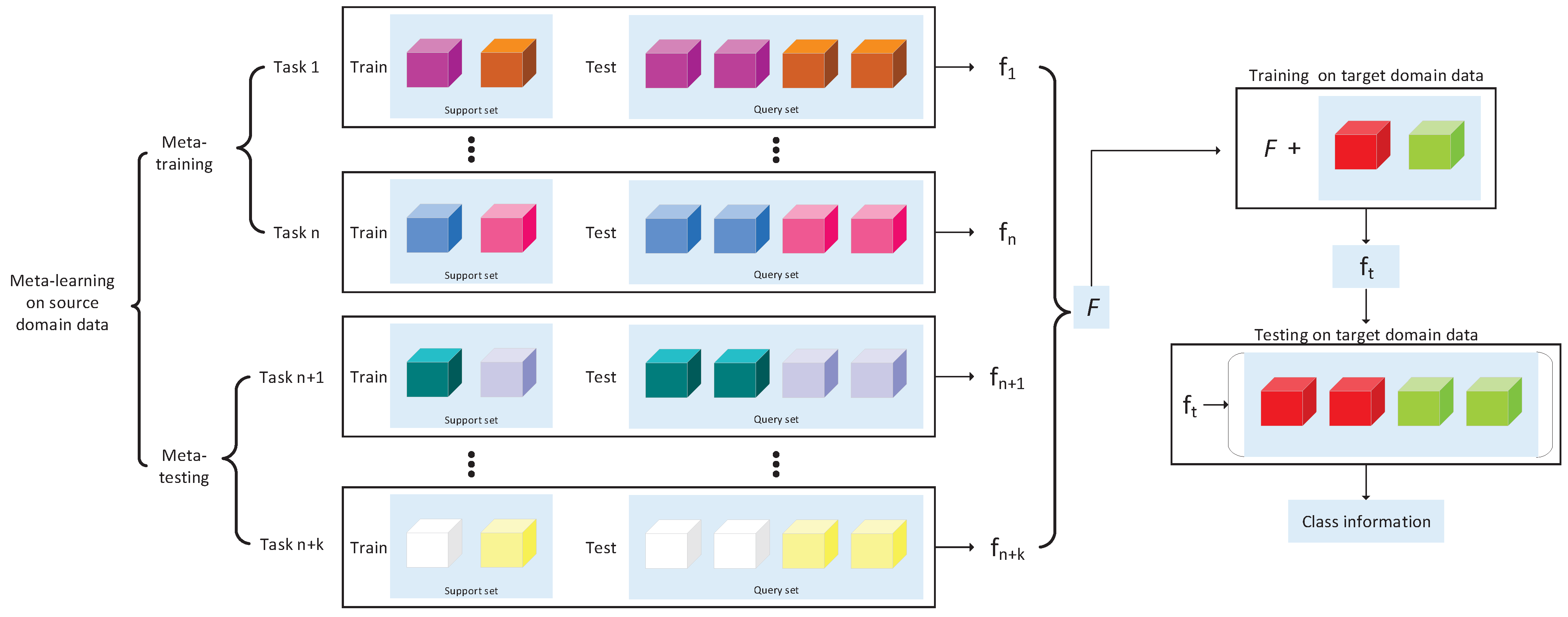
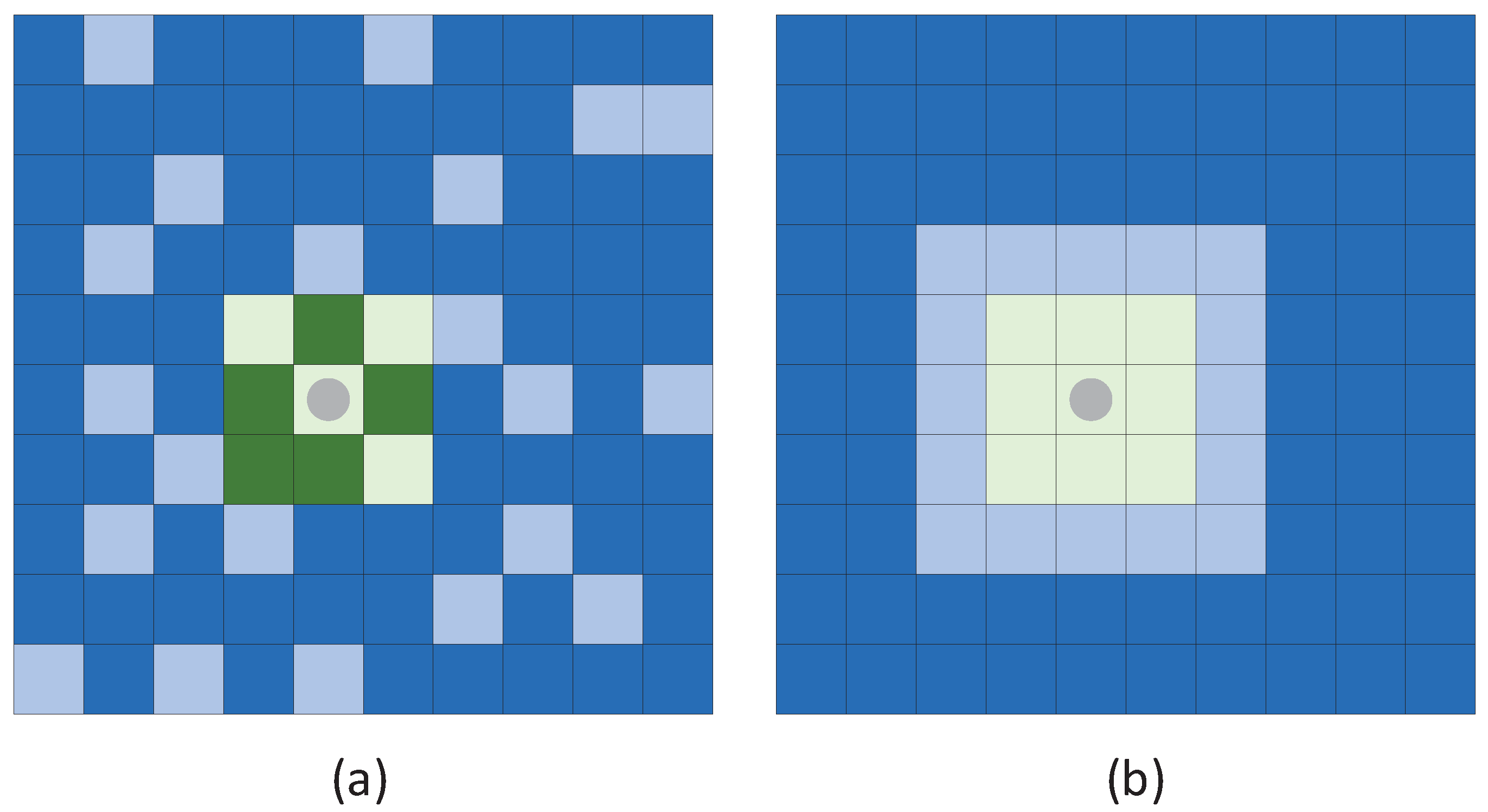
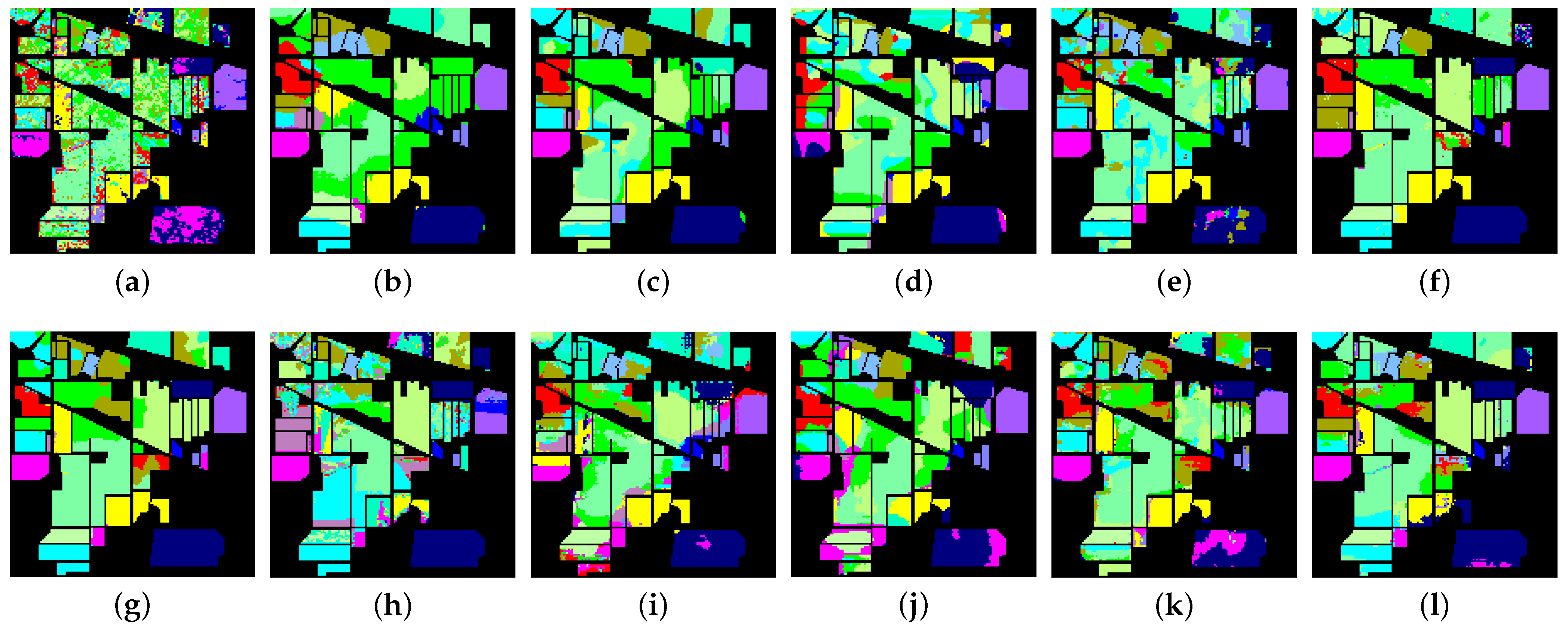
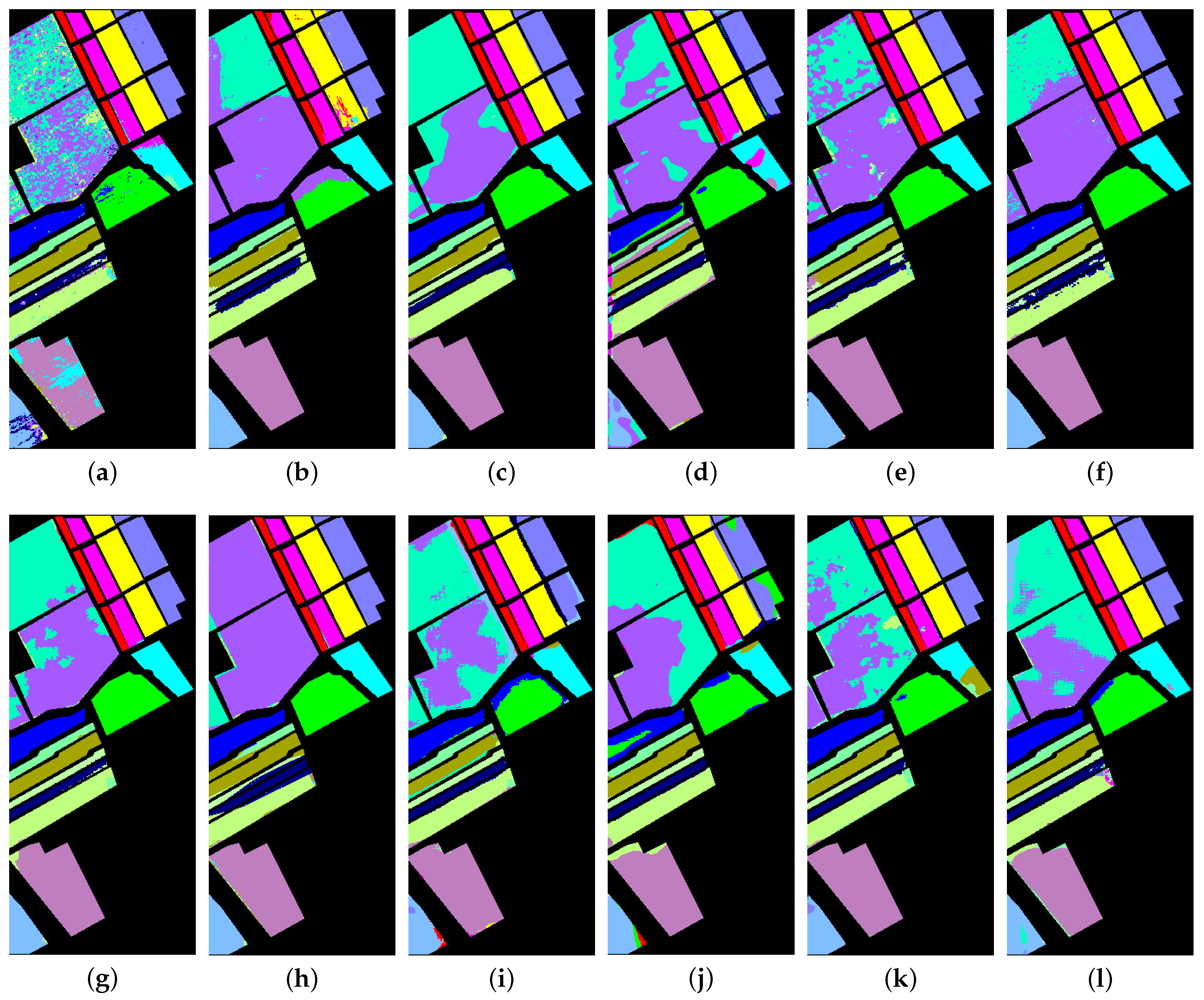
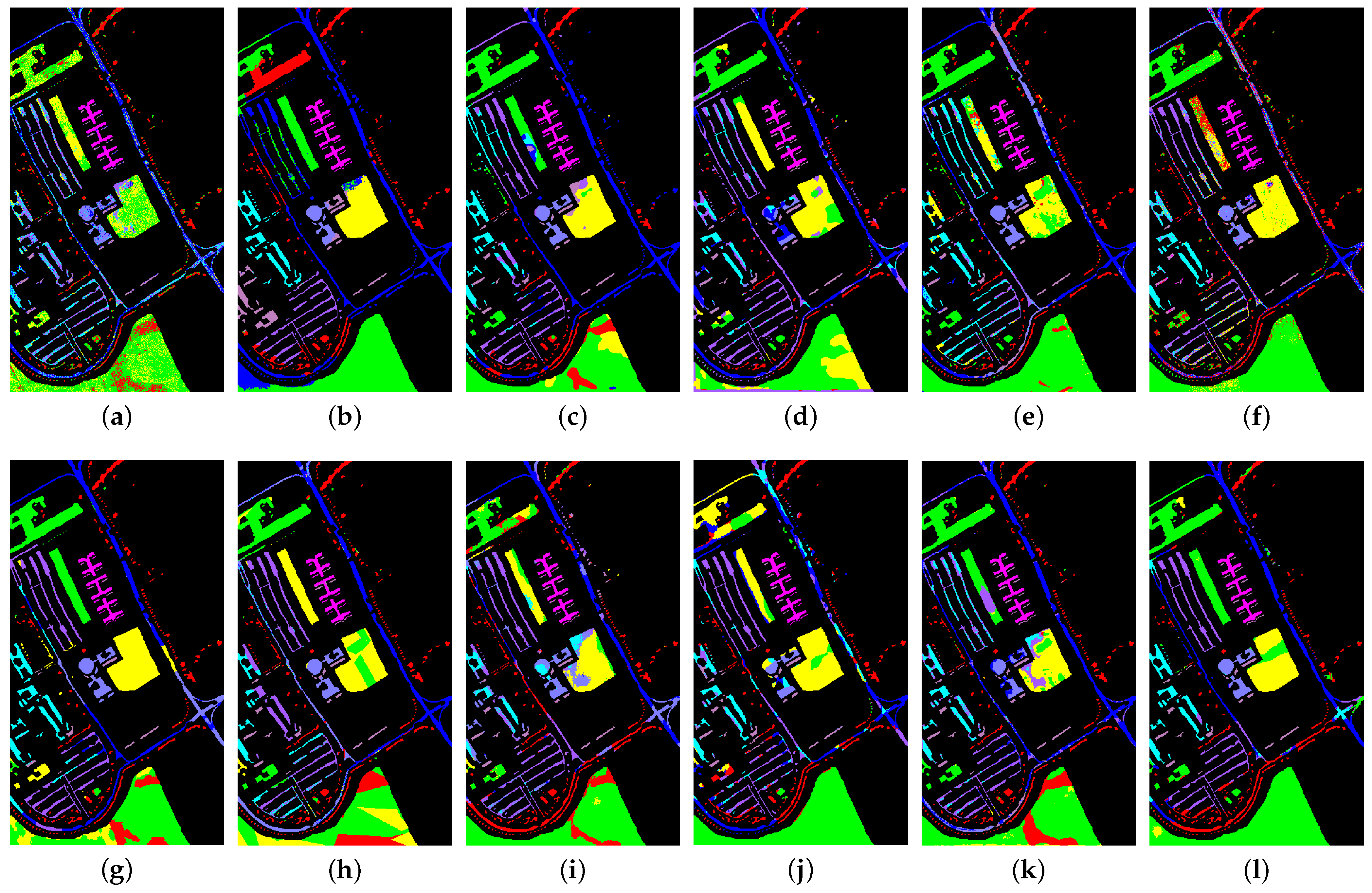
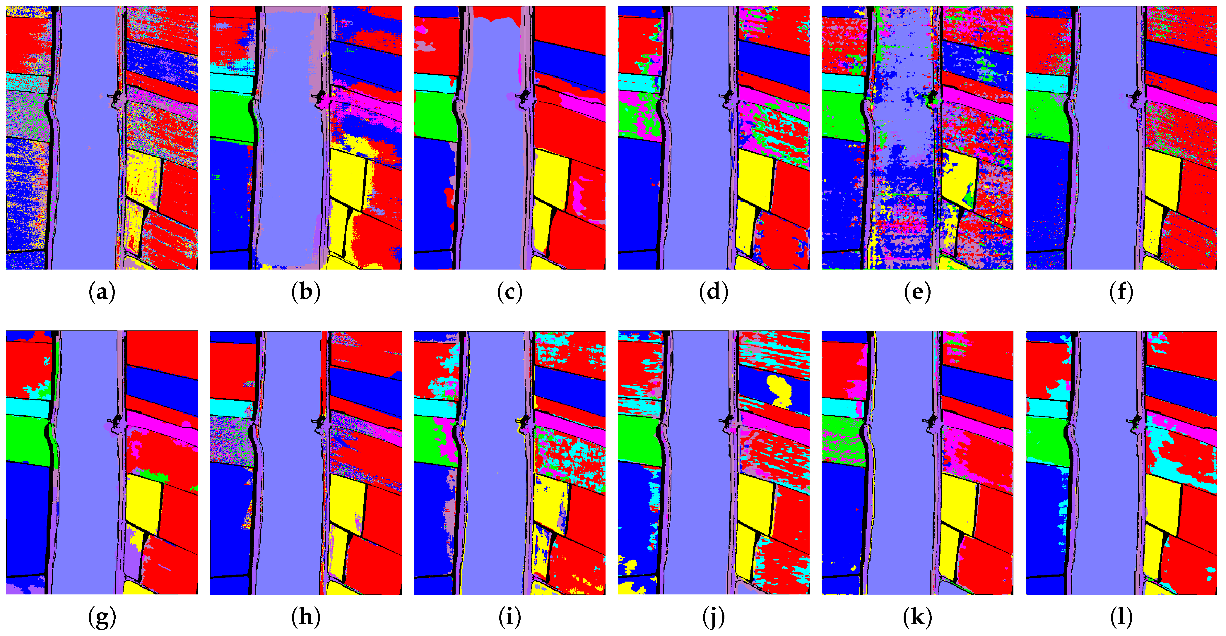
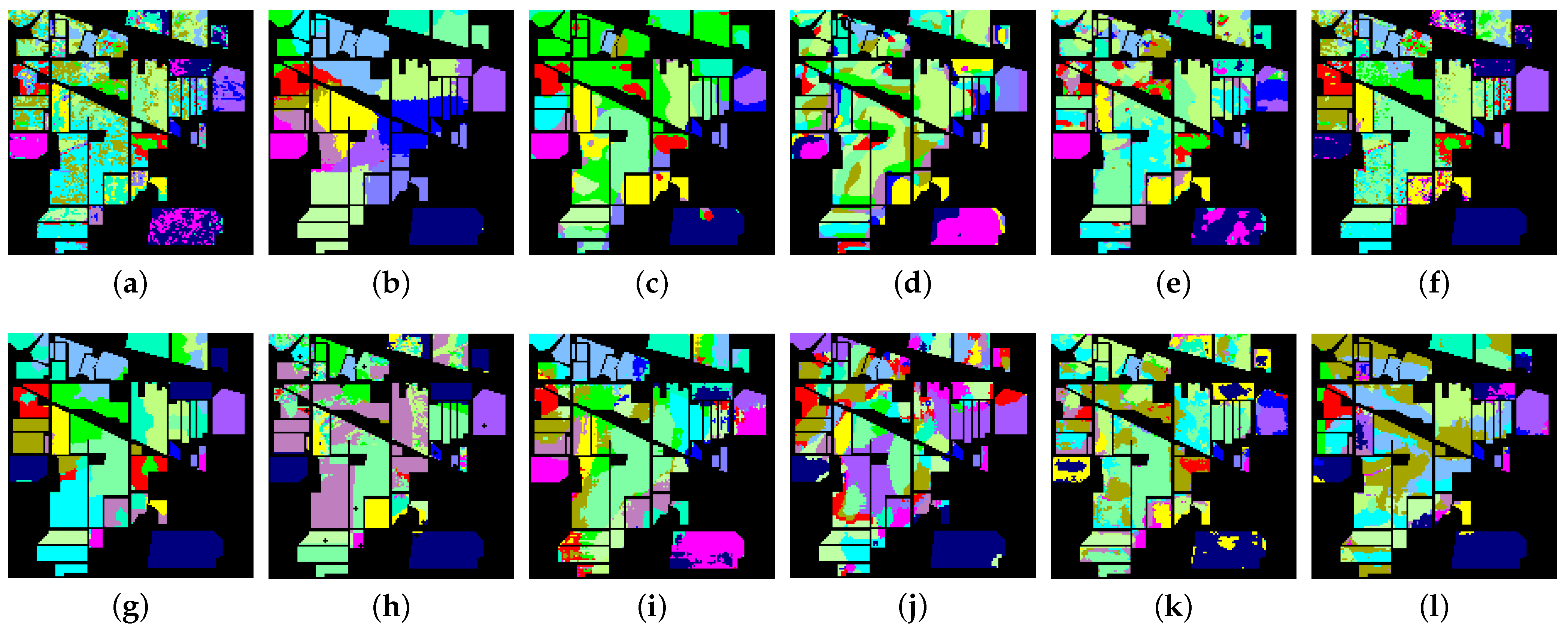
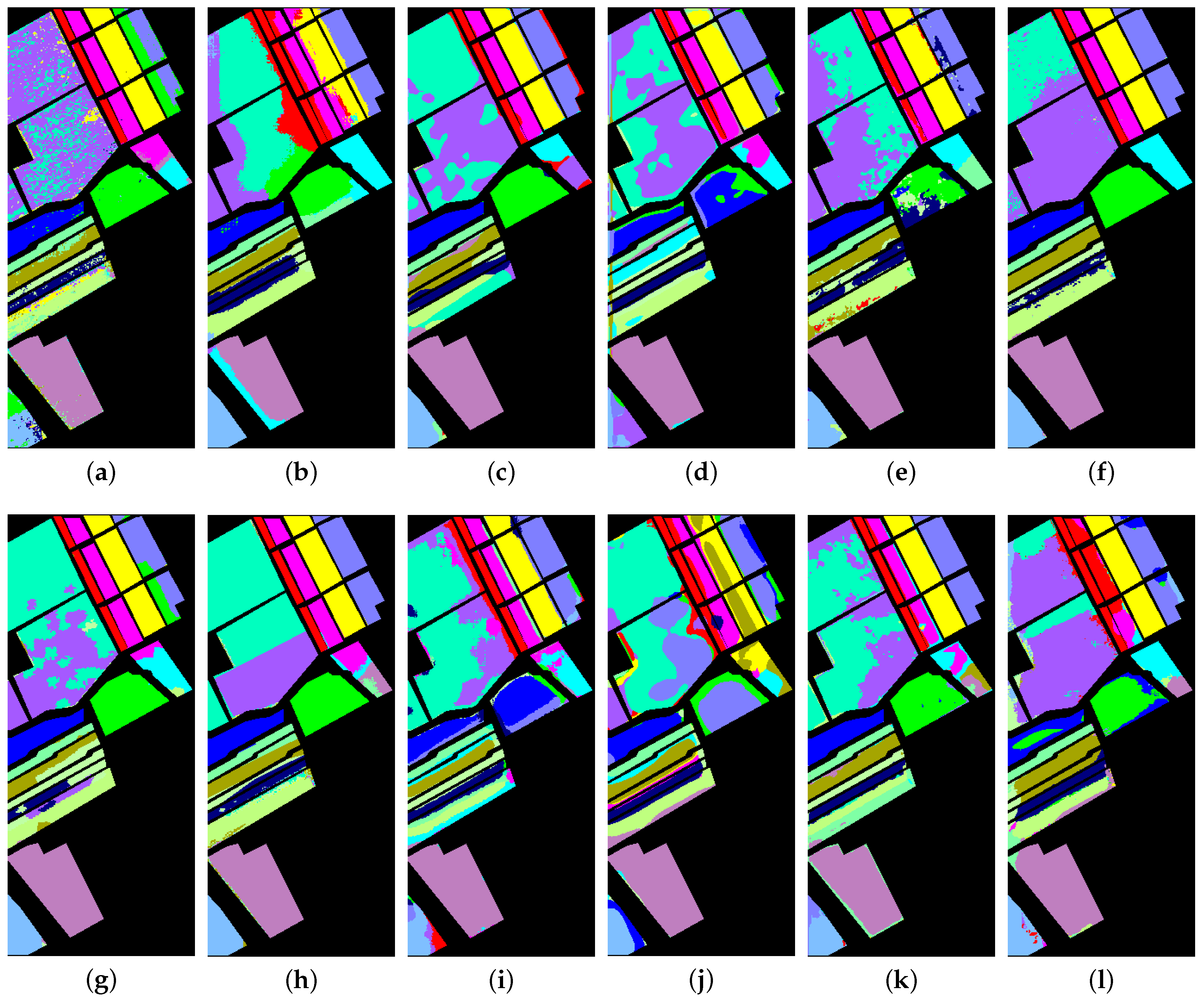
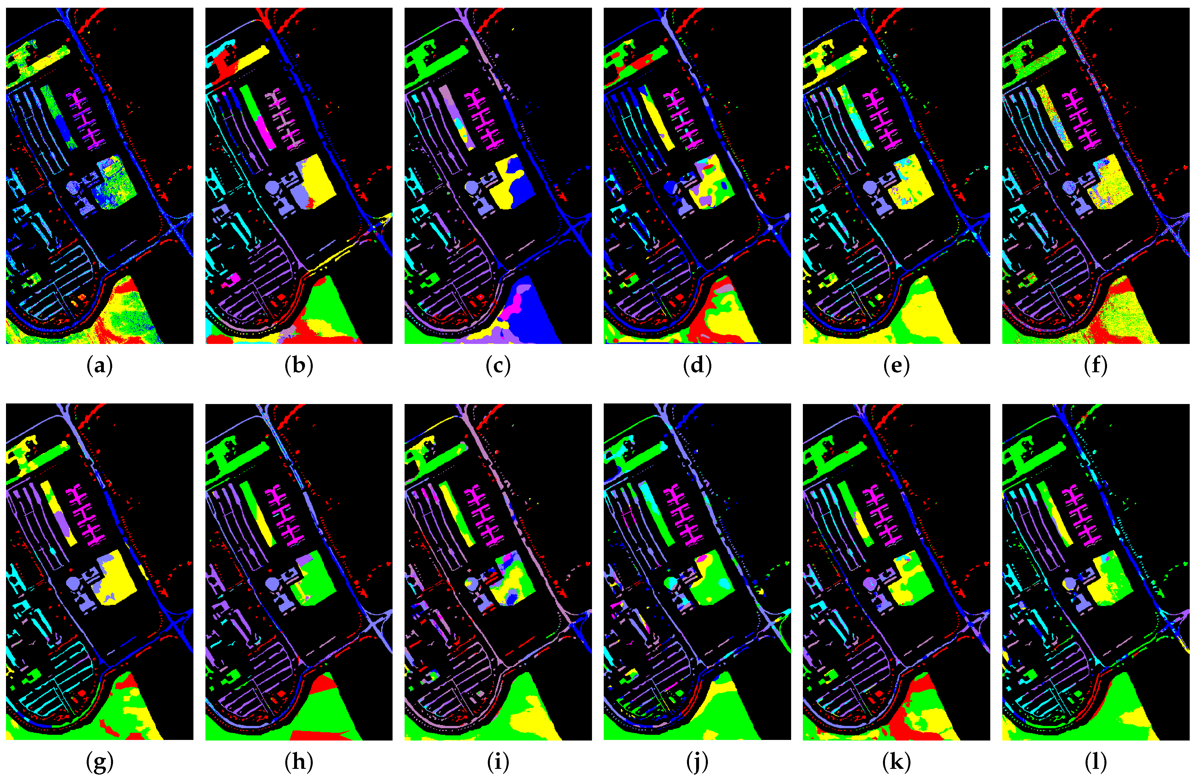
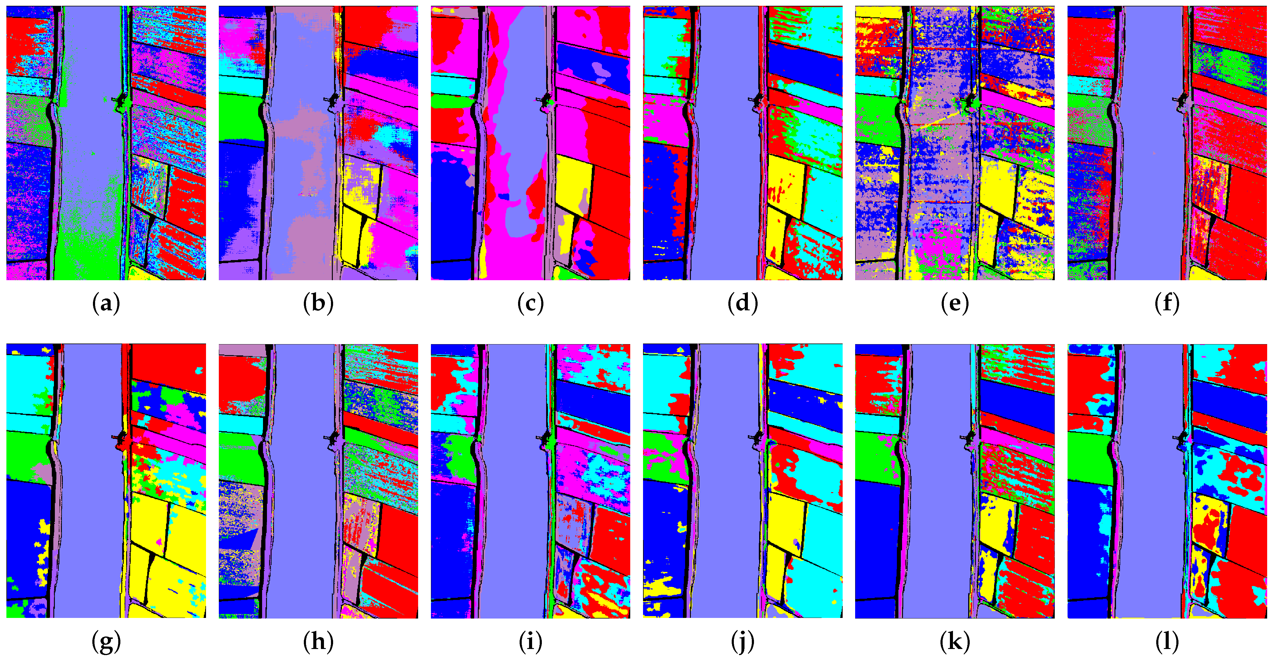
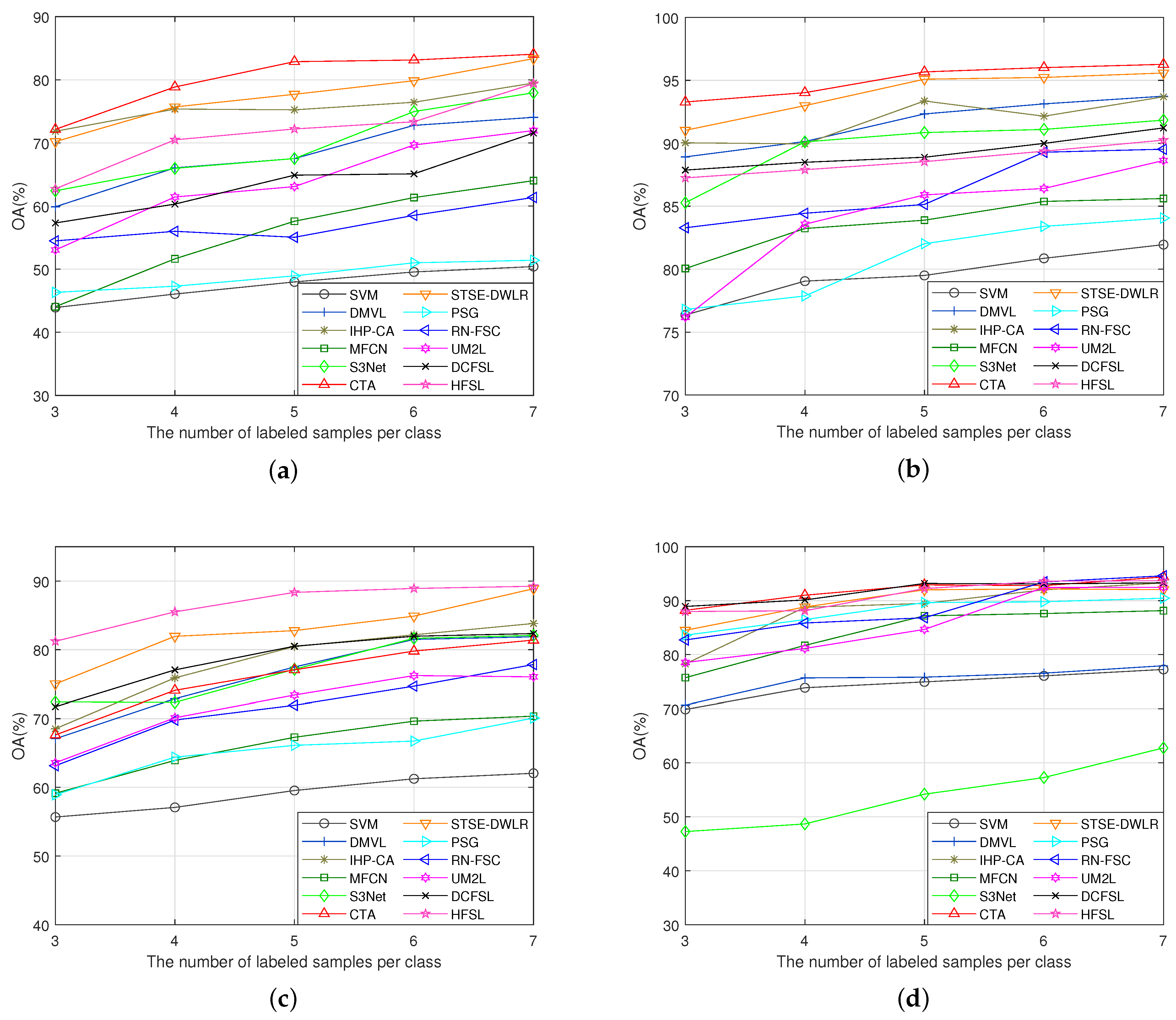
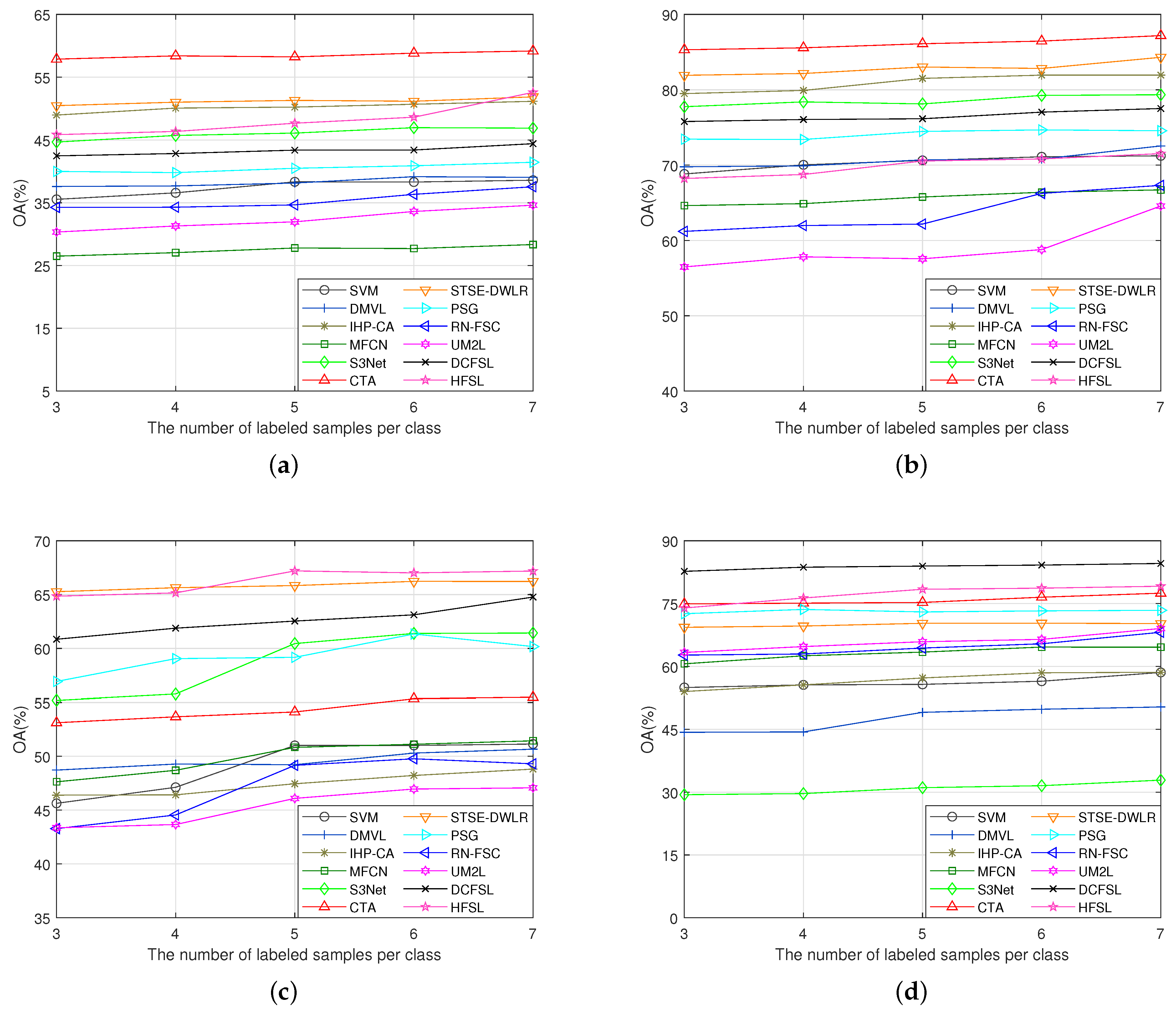
Table 1.
Brief introduction of the method in this experiment.
| Method | Year | |
|---|---|---|
| Based on intra-domain sample set (IS) | Support vector machine (SVM) [95] | 2002 |
| Deep multiview learning CNN (DMVL) [96] | 2021 | |
| Integrating hybrid pyramid feature fusion and coordinate attention CNN (IHP-CA) [58] | 2022 | |
| Minimalistic fully CNN (MFCN) [97] | 2022 | |
| S3Net: Spectral–spatial siamese network (S3Net) [35] | 2022 | |
| Based on intra-domain sample set expansion and pseudo-label generation (ISE-PG) | Spectral–spatial region growing co-traning approach and SVM (CTA) [69] | 2016 |
| Superpixel-guided training sample enlargement and distance-weighted linear regression classifier (STSE-DWLR) [68] | 2019 | |
| Polygon structure-guided training sample enlargement and SVM (PSG) [70] | 2022 | |
| Based on extra-domain sample set expansion and knowledge transfer (ESE-KT) | Deep relation network (RN-FSC) [29] | 2020 |
| Unsupervised Meta Learning CNN With Multiview Constraints (UM2L) [43] | 2022 | |
| Deep cross-domain few-shot learning CNN (DCFSL) [33] | 2022 | |
| Heterogeneous few-shot learning CNN (HFSL) [90] | 2022 |
Table 2.
The False color image, ground truth and the number of each category for four datasets.
| Indian Pines | Salinas Valley | Pavia University | WHU-Hi-LongKou | ||||||||
|---|---|---|---|---|---|---|---|---|---|---|---|
  |   |   |   | ||||||||
| Color | Land-cover type | Samples | Color | Land-cover type | Samples | Color | Land-cover type | Samples | Color | Land-cover type | Samples |
 | Background | 10,776 | | Background | 56,975 | | Background | 164,624 | | Background | 15,458 |
 | Alfalfa | 46 | | Brocoli-green-weeds-1 | 2009 | | Asphalt | 6631 | | Corn | 34,511 |
 | Corn-notill | 1428 | | Brocoli-green-weeds-2 | 3726 | | Meadows | 18,649 | | Cotton | 8374 |
 | Corn-minitill | 830 | | Fallow | 1976 | | Gravel | 2099 | | Sesame | 3031 |
 | Corn | 237 | | Fallow-rough-plow | 1394 | | Trees | 3064 | | Broad-leaf soybean | 63,212 |
 | Grass-pasture | 483 | | Fallow-smooth | 2678 | | Painted metal sheets | 1345 | | Narrow-leaf soybean | 4151 |
 | Grass-trees | 730 | | Stubble | 3959 | | Bare Soil | 5029 | | Rice | 11,854 |
 | Grass-pasture-mowed | 28 | | Celery | 3579 | | Bitumen | 1330 | | Water | 67,056 |
 | Hay-windrowed | 478 | | Grapes-untrained | 11,271 | | Self-Blocking Bricks | 3682 | | Roads and houses | 7124 |
 | Oats | 20 | | Soil-vinyard-develop | 6203 | | Shadows | 947 | | Mixed weed | 5229 |
 | Soybean-notill | 972 | | Corn-senesced-green-weeds | 3278 | ||||||
 | Soybean-mintill | 2455 | | Lettuce-romaine-4wk | 1068 | ||||||
 | Soybean-clean | 593 | | Lettuce-romaine-5wk | 1927 | ||||||
 | Wheat | 205 | | Lettuce-romaine-6wk | 916 | ||||||
 | Woods | 1265 | | Lettuce-romaine-7wk | 1070 | ||||||
 | Buildings-Grass-Trees-Drives | 386 | | Vinyard-untrained | 7268 | ||||||
 | Stone-Steel-Towers | 93 | | Vinyard-vertical-trellis | 1807 | ||||||
| Total samples | 21,025 | Total samples | 111,104 | Total samples | 207,400 | Total samples | 220,000 | ||||
Table 3.
Classification results of IP dataset under random sampling.
| Class | Methods | |||||||||||
|---|---|---|---|---|---|---|---|---|---|---|---|---|
| SVM | DMVL | IHP-CA | MFCN | S3Net | CTA | STSE-DWLR | PSG | RN-FSC | UM2L | DCFSL | HFSL | |
| Alfalfa | 28.19 | 32.78 | 61.62 | 26.51 | 99.76 | 99.14 | 98.05 | 71.76 | 25.62 | 63.63 | 94.63 | 99.27 |
| Corn-notill | 39.74 | 77.49 | 79.12 | 46.47 | 47.38 | 77.13 | 57.81 | 28.53 | 59.10 | 60.01 | 44.26 | 57.62 |
| Corn-mintill | 37.05 | 68.86 | 55.64 | 41.70 | 58.82 | 71.96 | 74.10 | 39.66 | 30.24 | 67.55 | 44.28 | 70.19 |
| Corn | 26.06 | 65.47 | 90.98 | 46.16 | 89.61 | 71.82 | 97.24 | 29.15 | 57.44 | 67.41 | 76.47 | 91.42 |
| Grass-pasture | 42.93 | 81.54 | 91.78 | 64.19 | 78.97 | 92.76 | 85.75 | 70.86 | 52.87 | 82.01 | 75.31 | 72.03 |
| Grass-trees | 80.92 | 66.07 | 33.52 | 77.75 | 95.45 | 90.89 | 92.36 | 90.33 | 84.54 | 43.46 | 84.70 | 79.86 |
| Grass-pasture-mowed | 23.70 | 20.30 | 99.11 | 24.16 | 100 | 58.77 | 96.52 | 41.69 | 38.29 | 89.40 | 98.26 | 100 |
| Hay-windrowed | 92.34 | 93.95 | 24.68 | 91.77 | 83.30 | 97.39 | 100 | 95.08 | 93.58 | 20.72 | 84.33 | 97.55 |
| Oats | 12.92 | 15.09 | 74.42 | 7.58 | 100 | 81.21 | 98.67 | 3.53 | 15.58 | 50.36 | 100 | 100 |
| Soybean-notill | 38.63 | 69.37 | 84.86 | 55.44 | 57.23 | 69.32 | 73.96 | 43.98 | 37.98 | 78.08 | 61.74 | 57.96 |
| Soybean-mintill | 56.25 | 79.28 | 59.51 | 64.40 | 58.13 | 88.50 | 66.73 | 59.48 | 54.70 | 56.18 | 61.40 | 60.86 |
| Soybean-clean | 22.23 | 64.15 | 74.22 | 38.82 | 60.41 | 75.66 | 73.18 | 27.55 | 56.37 | 64.83 | 45.60 | 69.90 |
| Wheat | 83.20 | 53.13 | 93.93 | 56.21 | 99.05 | 83.99 | 100 | 78.58 | 52.75 | 84.44 | 97.95 | 98.40 |
| Woods | 83.40 | 89.63 | 62.06 | 87.18 | 83.16 | 97.91 | 92.94 | 89.87 | 88.00 | 61.74 | 84.90 | 93.75 |
| Buildings-Grass-Trees-Drives | 27.96 | 72.82 | 59.21 | 60.61 | 76.27 | 94.07 | 99.74 | 42.97 | 50.55 | 43.50 | 66.61 | 90.10 |
| Stone-Steel-Towers | 85.20 | 23.72 | 52.16 | 52.71 | 99.43 | 90.61 | 91.93 | 99.74 | 26.83 | 41.17 | 98.86 | 95.80 |
| OA (%) | 47.98 ± 2.60 | 67.52 ± 5.07 | 75.24 ± 3.11 | 57.59 ± 3.44 | 67.52 ± 3.41 | 82.87 ± 1.94 | 77.70 ± 4.24 | 48.94 ± 6.63 | 55.05 ± 5.22 | 63.08 ± 4.04 | 64.89 ± 2.57 | 72.21 ± 4.05 |
| AA (%) | 48.79 ± 1.81 | 60.86 ± 4.45 | 68.86 ± 3.63 | 52.61 ± 3.56 | 80.43 ± 1.35 | 83.82 ± 3.42 | 87.43 ± 1.86 | 57.05 ± 3.98 | 51.53 ± 3.21 | 60.87 ± 3.16 | 76.21 ± 2.13 | 83.42 ± 2.39 |
| Kappa × 100 | 41.91 ± 2.57 | 63.67 ± 5.36 | 72.22 ± 3.35 | 52.37 ± 3.61 | 63.57 ± 3.58 | 80.56 ± 2.18 | 74.96 ± 4.60 | 43.43 ± 6.44 | 50.02 ± 5.53 | 58.83 ± 4.29 | 60.37 ± 2.89 | 68.75 ± 4.43 |
Table 4.
Classification results of SV dataset under random sampling.
| Class | Methods | |||||||||||
|---|---|---|---|---|---|---|---|---|---|---|---|---|
| SVM | DMVL | IHP-CA | MFCN | S3Net | CTA | STSE-DWLR | PSG | RN-FSC | UM2L | DCFSL | HFSL | |
| Brocoli-green-weeds-1 | 89.94 | 97.46 | 99.92 | 86.27 | 99.91 | 100 | 99.40 | 97.90 | 83.09 | 94.28 | 99.32 | 99.27 |
| Brocoli-green-weeds-2 | 97.36 | 99.89 | 99.63 | 92.43 | 94.24 | 99.93 | 99.85 | 99.71 | 95.35 | 94.80 | 99.26 | 93.03 |
| Fallow | 84.33 | 95.35 | 84.03 | 91.50 | 96.94 | 93.66 | 96.91 | 96.42 | 91.24 | 84.32 | 88.98 | 96.41 |
| Fallow-rough-plow | 99.31 | 69.46 | 99.00 | 91.99 | 98.80 | 92.01 | 99.82 | 98.96 | 90.29 | 93.31 | 99.61 | 99.59 |
| Fallow-smooth | 92.13 | 93.10 | 99.26 | 93.79 | 97.52 | 99.39 | 98.68 | 92.09 | 94.19 | 97.83 | 91.67 | 96.45 |
| Stubble | 97.13 | 94.89 | 97.47 | 99.78 | 99.28 | 99.78 | 99.92 | 97.08 | 99.77 | 95.19 | 99.34 | 99.65 |
| Celery | 96.58 | 97.98 | 94.37 | 90.91 | 98.89 | 99.66 | 99.80 | 99.42 | 93.08 | 88.90 | 99.34 | 97.70 |
| Grapes-untrained | 66.48 | 95.45 | 98.93 | 83.63 | 81.66 | 92.39 | 86.16 | 79.22 | 87.73 | 96.83 | 75.39 | 76.59 |
| Soil-vinyard-develop | 97.41 | 99.99 | 97.65 | 94.97 | 99.71 | 98.74 | 96.75 | 93.01 | 97.98 | 91.77 | 99.39 | 93.12 |
| Corn-senesced-green-weeds | 76.63 | 98.97 | 93.61 | 83.28 | 92.57 | 96.41 | 93.77 | 91.14 | 91.85 | 94.55 | 81.41 | 90.90 |
| Lettuce-romaine-4wk | 76.39 | 93.79 | 98.74 | 79.56 | 99.53 | 97.64 | 97.76 | 66.28 | 91.01 | 89.67 | 98.17 | 98.86 |
| Lettuce-romaine-5wk | 88.41 | 99.39 | 93.92 | 88.47 | 88.67 | 99.45 | 97.13 | 78.33 | 93.44 | 91.04 | 99.34 | 98.13 |
| Lettuce-romaine-6wk | 91.20 | 88.24 | 84.93 | 78.45 | 97.96 | 89.18 | 97.65 | 72.47 | 84.11 | 86.07 | 99.28 | 99.09 |
| Lettuce-romaine-7wk | 79.13 | 67.43 | 78.56 | 79.44 | 91.57 | 85.53 | 94.75 | 63.24 | 85.73 | 63.13 | 98.08 | 96.35 |
| Vinyard-untrained | 46.37 | 84.52 | 99.79 | 64.50 | 75.39 | 91.98 | 94.60 | 45.34 | 62.53 | 88.32 | 75.11 | 57.86 |
| Vinyard-vertical-trellis | 91.23 | 96.75 | 99.23 | 78.43 | 96.10 | 99.84 | 99.17 | 99.39 | 83.38 | 87.76 | 89.92 | 95.27 |
| OA (%) | 79.50 ± 3.67 | 92.33 ± 2.52 | 93.36 ± 1.49 | 83.89 ± 2.64 | 90.85 ± 1.29 | 95.67 ± 0.60 | 95.09 ± 2.47 | 82.02 ± 7.02 | 85.14 ± 4.30 | 85.90 ± 4.43 | 88.89 ± 2.16 | 88.54 ± 2.11 |
| AA (%) | 85.63 ± 2.23 | 92.04 ± 1.93 | 94.93 ± 1.20 | 86.09 ± 2.16 | 94.29 ± 1.20 | 95.98 ± 0.82 | 97.01 ± 1.59 | 85.63 ± 3.69 | 89.04 ± 2.07 | 89.86 ± 2.32 | 93.35 ± 1.37 | 93.71 ± 1.09 |
| Kappa × 100 | 77.26 ± 4.47 | 91.48 ± 2.78 | 92.63 ± 1.65 | 82.17 ± 2.89 | 89.82 ± 1.44 | 95.18 ± 0.45 | 94.54 ± 2.75 | 80.01 ± 7.74 | 87.63 ± 3.67 | 84.42 ± 4.84 | 87.66 ± 2.36 | 87.26 ± 3.80 |
Table 5.
Classification results of PU dataset under random sampling.
| Class | Methods | |||||||||||
|---|---|---|---|---|---|---|---|---|---|---|---|---|
| SVM | DMVL | IHP-CA | MFCN | S3Net | CTA | STSE-DWLR | PSG | RN-FSC | UM2L | DCFSL | HFSL | |
| Asphalt | 72.42 | 71.16 | 98.03 | 81.15 | 81.76 | 97.35 | 84.19 | 84.49 | 86.15 | 93.81 | 73.99 | 75.46 |
| Meadows | 82.96 | 93.94 | 64.11 | 87.59 | 75.51 | 92.96 | 73.72 | 86.92 | 97.43 | 55.88 | 84.80 | 90.49 |
| Gravel | 40.71 | 81.41 | 60.73 | 46.70 | 70.08 | 61.96 | 99.58 | 67.29 | 43.66 | 54.64 | 60.03 | 75.86 |
| trees | 67.90 | 47.77 | 92.29 | 65.85 | 85.83 | 45.43 | 85.89 | 73.02 | 71.61 | 79.33 | 93.01 | 95.28 |
| Painted metal sheets | 99.99 | 86.21 | 78.12 | 98.21 | 99.93 | 73.21 | 99.80 | 90.56 | 95.18 | 54.86 | 99.23 | 99.81 |
| Bare soil | 27.83 | 94.21 | 90.53 | 42.44 | 64.17 | 72.87 | 99.95 | 40.32 | 46.00 | 70.56 | 75.14 | 86.65 |
| Bitumen | 41.89 | 82.98 | 64.25 | 54.08 | 95.14 | 83.83 | 99.98 | 51.30 | 44.50 | 75.41 | 79.54 | 91.84 |
| Self-blocking bricks | 54.84 | 81.75 | 71.63 | 66.05 | 72.45 | 70.81 | 82.95 | 62.14 | 75.04 | 66.91 | 68.25 | 96.28 |
| Shadows | 81.75 | 23.81 | 87.46 | 91.09 | 94.90 | 71.31 | 64.16 | 89.83 | 76.27 | 88.08 | 97.73 | 99.06 |
| OA (%) | 59.54 ± 2.13 | 77.48 ± 7.24 | 80.46 ± 6.22 | 67.29 ± 5.37 | 77.15 ± 8.04 | 77.07 ± 5.13 | 82.78 ± 7.72 | 66.12 ± 8.55 | 71.94 ± 4.54 | 73.41 ± 6.23 | 80.51 ± 2.64 | 88.35 ± 3.58 |
| AA (%) | 63.36 ± 3.19 | 73.69 ± 4.77 | 78.84 ± 5.35 | 70.35 ± 3.92 | 82.19 ± 3.15 | 74.41 ± 3.52 | 87.80 ± 3.92 | 72.21 ± 7.09 | 70.93 ± 3.38 | 71.01 ± 3.78 | 81.30 ± 1.64 | 90.08 ± 2.26 |
| Kappa × 100 | 49.49 ± 2.13 | 71.14 ± 8.12 | 75.30 ± 7.45 | 59.21 ± 6.07 | 71.02 ± 8.89 | 70.88 ± 5.90 | 78.49 ± 8.84 | 58.02 ± 8.85 | 64.92 ± 5.11 | 66.66 ± 7.05 | 74.80 ± 3.12 | 84.83 ± 4.42 |
Table 6.
Classification results of LK dataset under random sampling.
| Class | Methods | |||||||||||
|---|---|---|---|---|---|---|---|---|---|---|---|---|
| SVM | DMVL | IHP-CA | MFCN | S3Net | CTA | STSE-DWLR | PSG | RN-FSC | UM2L | DCFSL | HFSL | |
| Corn | 79.49 | 82.11 | 85.39 | 92.87 | 69.47 | 95.36 | 94.51 | 93.74 | 96.02 | 91.00 | 98.34 | 98.17 |
| Cotton | 26.58 | 91.56 | 91.20 | 61.56 | 87.28 | 72.26 | 97.04 | 51.42 | 86.79 | 24.33 | 87.96 | 93.85 |
| Sesame | 27.27 | 60.29 | 91.01 | 52.55 | 95.87 | 65.65 | 99.09 | 59.75 | 32.16 | 95.46 | 87.22 | 83.34 |
| Broad-leaf soybean | 93.11 | 86.58 | 58.25 | 96.06 | 54.63 | 96.88 | 87.22 | 97.30 | 97.07 | 50.17 | 88.40 | 82.73 |
| Narrow-leaf soybean | 27.30 | 44.23 | 97.26 | 35.12 | 93.80 | 56.83 | 94.23 | 66.72 | 55.25 | 77.10 | 89.56 | 94.27 |
| Rice | 78.71 | 76.33 | 99.07 | 95.74 | 78.64 | 98.71 | 95.57 | 94.05 | 72.51 | 99.32 | 91.94 | 92.46 |
| Water | 99.99 | 97.69 | 66.02 | 99.78 | 47.86 | 99.75 | 97.58 | 98.80 | 99.71 | 77.36 | 99.87 | 99.64 |
| Roads and houses | 50.51 | 30.80 | 41.49 | 86.28 | 41.99 | 74.12 | 67.97 | 81.64 | 74.06 | 62.77 | 76.18 | 84.20 |
| Mixed weed | 21.65 | 23.46 | 97.75 | 64.27 | 40.07 | 88.80 | 72.72 | 59.47 | 59.61 | 94.25 | 72.09 | 84.51 |
| OA (%) | 74.94 ± 2.85 | 75.82 ± 2.23 | 89.49 ± 4.51 | 87.19 ± 5.61 | 58.23 ± 4.82 | 92.92 ± 1.62 | 92.01 ± 2.39 | 89.64 ± 3.21 | 86.83 ± 2.89 | 84.67 ± 4.91 | 93.19 ± 2.66 | 92.24 ± 4.29 |
| AA (%) | 56.07 ± 2.36 | 65.90 ± 2.01 | 80.83 ± 2.71 | 76.03 ± 5.28 | 67.73 ± 2.42 | 83.15 ± 2.96 | 89.55 ± 1.38 | 78.10 ± 5.10 | 74.80 ± 3.29 | 74.64 ± 3.73 | 87.95 ± 2.91 | 90.35 ± 3.45 |
| Kappa × 100 | 68.39 ± 3.37 | 69.57 ± 2.59 | 86.29 ± 5.41 | 83.65 ± 6.89 | 48.70 ± 4.70 | 90.82 ± 2.07 | 89.70 ± 2.98 | 86.59 ± 4.03 | 83.23 ± 3.50 | 80.61 ± 6.00 | 91.15 ± 3.39 | 90.23 ± 5.53 |
Table 7.
Classification results of IP dataset under disjointed sampling.
| Class | Methods | |||||||||||
|---|---|---|---|---|---|---|---|---|---|---|---|---|
| SVM | DMVL | IHP-CA | MFCN | S3Net | CTA | STSE-DWLR | PSG | RN-FSC | UM2L | DCFSL | HFSL | |
| Alfalfa | 15.18 | 8.07 | 60.15 | 7.32 | 97.56 | 82.02 | 97.56 | 65.78 | 15.59 | 41.10 | 89.02 | 96.34 |
| Corn-notill | 37.80 | 73.47 | 37.67 | 27.16 | 25.81 | 62.18 | 31.19 | 39.18 | 42.57 | 34.74 | 18.95 | 33.31 |
| Corn-mintill | 24.54 | 64.02 | 33.26 | 29.41 | 30.05 | 51.27 | 37.05 | 26.13 | 31.22 | 39.40 | 28.22 | 23.04 |
| Corn | 18.20 | 49.21 | 87.56 | 21.99 | 58.75 | 41.98 | 72.89 | 24.10 | 30.20 | 30.27 | 41.90 | 53.84 |
| Grass-pasture | 51.48 | 68.29 | 77.49 | 22.62 | 49.81 | 70.37 | 53.45 | 68.01 | 45.36 | 57.28 | 41.86 | 42.97 |
| Grass-trees | 78.98 | 58.88 | 18.13 | 47.44 | 83.53 | 76.53 | 62.83 | 91.58 | 64.93 | 13.60 | 66.18 | 41.75 |
| Grass-pasture-mowed | 10.63 | 14.07 | 98.44 | 6.26 | 100 | 56.09 | 99.13 | 28.17 | 12.68 | 63.30 | 92.61 | 96.52 |
| Hay-windrowed | 89.04 | 77.28 | 4.94 | 60.94 | 42.18 | 88.51 | 88.60 | 95.53 | 90.19 | 5.45 | 42.77 | 71.78 |
| Oats | 8.46 | 13.83 | 61.68 | 3.05 | 98.67 | 36.08 | 100 | 0.91 | 4.34 | 38.00 | 98.04 | 94.75 |
| Soybean-notill | 37.53 | 63.20 | 64.76 | 25.62 | 46.69 | 48.09 | 54.87 | 46.09 | 34.36 | 62.89 | 45.69 | 39.80 |
| Soybean-mintill | 51.72 | 82.17 | 47.08 | 47.96 | 32.97 | 75.47 | 31.19 | 59.03 | 53.43 | 28.32 | 38.89 | 46.79 |
| Soybean-clean | 16.51 | 53.99 | 51.93 | 13.87 | 29.22 | 46.92 | 32.59 | 25.28 | 34.62 | 32.12 | 15.07 | 30.09 |
| Wheat | 76.07 | 33.92 | 84.00 | 23.24 | 98.55 | 62.30 | 100 | 68.42 | 18.11 | 59.80 | 79.50 | 85.55 |
| Woods | 77.63 | 82.27 | 51.11 | 69.46 | 70.47 | 86.14 | 79.38 | 91.90 | 85.76 | 43.71 | 75.48 | 74.10 |
| Buildings-Grass-Trees-Drives | 21.89 | 49.71 | 52.37 | 40.44 | 56.40 | 70.23 | 85.51 | 31.47 | 40.78 | 25.03 | 48.19 | 64.28 |
| Stone-Steel-Towers | 85.81 | 14.70 | 29.00 | 13.81 | 96.48 | 43.71 | 90.00 | 97.92 | 18.62 | 8.97 | 90.91 | 92.50 |
| OA (%) | 38.33 ± 3.68 | 38.14 ± 9.94 | 50.24 ± 6.16 | 27.79 ± 7.00 | 46.10 ± 5.86 | 58.24 ± 9.05 | 51.31 ± 4.95 | 40.49 ± 7.38 | 34.66 ± 7.66 | 31.96 ± 6.79 | 43.38 ± 5.71 | 47.67 ± 5.38 |
| AA (%) | 43.84 ± 2.52 | 50.44 ± 10.70 | 53.72 ± 3.48 | 28.79 ± 3.80 | 63.57 ± 3.12 | 62.36 ± 4.26 | 69.77 ± 2.59 | 53.72 ± 4.07 | 38.92 ± 2.79 | 36.50 ± 2.64 | 57.08 ± 3.21 | 61.70 ± 4.43 |
| Kappa× 100 | 32.29 ± 3.55 | 34.50 ± 9.36 | 45.14 ± 6.04 | 21.95 ± 6.44 | 40.61 ± 5.89 | 53.48 ± 9.30 | 46.48 ± 4.86 | 34.88 ± 6.77 | 29.03 ± 7.57 | 26.66 ± 6.67 | 37.12 ± 5.49 | 41.77 ± 5.52 |
Table 8.
Classification results of SV dataset under disjointed sampling.
| Class | Methods | |||||||||||
|---|---|---|---|---|---|---|---|---|---|---|---|---|
| SVM | DMVL | IHP-CA | MFCN | S3Net | CTA | STSE-DWLR | PSG | RN-FSC | UM2L | DCFSL | HFSL | |
| Brocoli-green-weeds-1 | 86.03 | 78.32 | 98.69 | 66.17 | 98.56 | 99.98 | 99.40 | 94.57 | 41.16 | 64.30 | 96.84 | 71.44 |
| Brocoli-green-weeds-2 | 86.26 | 91.15 | 90.52 | 71.90 | 84.40 | 99.57 | 98.63 | 93.39 | 61.30 | 49.96 | 89.78 | 73.76 |
| Fallow | 71.71 | 72.68 | 74.97 | 62.75 | 61.72 | 88.31 | 60.39 | 88.93 | 66.79 | 53.45 | 48.21 | 55.84 |
| Fallow-rough-plow | 99.27 | 46.10 | 86.55 | 86.85 | 90.23 | 84.59 | 99.73 | 98.94 | 63.95 | 78.52 | 99.34 | 96.02 |
| Fallow-smooth | 81.30 | 82.83 | 99.66 | 81.50 | 96.30 | 85.97 | 97.55 | 85.20 | 72.46 | 87.48 | 84.01 | 87.36 |
| Stubble | 91.40 | 83.69 | 96.17 | 99.53 | 98.69 | 99.63 | 99.92 | 93.17 | 98.59 | 77.66 | 99.34 | 97.55 |
| Celery | 92.48 | 92.05 | 80.64 | 82.47 | 90.97 | 99.60 | 86.54 | 94.71 | 72.55 | 68.62 | 98.19 | 77.01 |
| Grapes-untrained | 60.75 | 88.51 | 95.69 | 58.70 | 59.42 | 87.89 | 69.69 | 59.23 | 63.23 | 88.49 | 52.99 | 58.63 |
| Soil-vinyard-develop | 90.63 | 99.93 | 97.78 | 89.67 | 97.12 | 97.60 | 95.12 | 90.80 | 92.12 | 69.54 | 96.00 | 79.97 |
| Corn-senesced-green-weeds | 72.05 | 82.02 | 84.84 | 70.04 | 61.19 | 93.54 | 72.03 | 84.57 | 70.34 | 52.35 | 51.83 | 59.15 |
| Lettuce-romaine-4wk | 55.62 | 69.25 | 76.35 | 45.50 | 95.93 | 69.43 | 95.78 | 62.92 | 49.09 | 63.34 | 78.02 | 95.54 |
| Lettuce-romaine-5wk | 77.05 | 85.82 | 57.61 | 70.83 | 67.26 | 91.37 | 70.43 | 65.59 | 62.95 | 63.91 | 95.29 | 80.00 |
| Lettuce-romaine-6wk | 81.12 | 59.47 | 62.82 | 43.87 | 75.93 | 79.14 | 96.36 | 56.33 | 59.44 | 48.90 | 96.84 | 90.96 |
| Lettuce-romaine-7wk | 66.39 | 51.45 | 58.39 | 60.40 | 78.37 | 72.19 | 84.28 | 68.27 | 61.80 | 43.54 | 96.08 | 79.16 |
| Vinyard-untrained | 41.68 | 71.68 | 97.72 | 46.36 | 67.28 | 64.20 | 69.76 | 33.56 | 54.53 | 41.93 | 58.67 | 51.19 |
| Vinyard-vertical-trellis | 61.50 | 70.86 | 99.70 | 51.51 | 81.37 | 99.53 | 92.37 | 95.06 | 61.57 | 48.27 | 78.89 | 62.86 |
| OA (%) | 70.62 ± 4.61 | 70.69 ± 15.06 | 81.51 ± 5.59 | 65.76 ± 4.56 | 78.12 ± 4.92 | 86.11 ± 3.70 | 83.02 ± 4.70 | 74.47 ± 9.26 | 62.17 ± 5.23 | 57.56 ± 6.93 | 76.15 ± 3.61 | 70.54 ± 2.83 |
| AA (%) | 75.95 ± 4.40 | 76.61 ± 6.27 | 84.88 ± 2.38 | 68.01 ± 5.91 | 81.55 ± 3.53 | 88.28 ± 2.59 | 86.75 ± 2.36 | 79.08 ± 7.30 | 65.74 ± 3.45 | 62.52 ± 5.22 | 82.52 ± 3.96 | 76.03 ± 4.76 |
| Kappa × 100 | 67.48 ± 5.00 | 68.16 ± 16.05 | 72.02 ± 6.27 | 62.14 ± 4.92 | 75.76 ± 5.39 | 84.62 ± 4.06 | 81.15 ± 5.17 | 71.64 ± 10.20 | 68.19 ± 4.86 | 53.85 ± 7.06 | 73.58 ± 4.01 | 67.97 ± 3.53 |
Table 9.
Classification results of PU dataset under disjointed sampling.
| Class | Methods | |||||||||||
|---|---|---|---|---|---|---|---|---|---|---|---|---|
| SVM | DMVL | IHP-CA | MFCN | S3Net | CTA | STSE-DWLR | PSG | RN-FSC | UM2L | DCFSL | HFSL | |
| Asphalt | 56.84 | 51.33 | 96.31 | 51.03 | 41.96 | 82.45 | 60.04 | 94.86 | 56.04 | 78.51 | 65.57 | 52.69 |
| Meadows | 79.89 | 89.90 | 50.44 | 77.24 | 61.50 | 85.28 | 54.72 | 83.01 | 82.76 | 22.04 | 64.40 | 77.76 |
| Gravel | 33.46 | 39.30 | 62.73 | 17.25 | 47.38 | 42.89 | 87.60 | 48.73 | 38.03 | 27.04 | 49.32 | 24.57 |
| trees | 51.26 | 24.09 | 77.03 | 50.80 | 80.37 | 37.04 | 74.00 | 55.46 | 37.74 | 47.39 | 87.40 | 82.12 |
| Painted metal sheets | 100 | 54.45 | 51.18 | 74.30 | 99.59 | 56.52 | 85.77 | 89.52 | 75.79 | 39.17 | 98.31 | 99.94 |
| Bare soil | 33.21 | 59.93 | 62.49 | 40.77 | 41.32 | 40.67 | 91.00 | 31.20 | 36.51 | 21.10 | 33.39 | 43.48 |
| Bitumen | 39.13 | 52.64 | 34.68 | 29.42 | 97.67 | 62.36 | 99.46 | 44.88 | 42.24 | 47.70 | 71.58 | 52.61 |
| Self-blocking bricks | 54.82 | 52.51 | 42.15 | 46.74 | 69.67 | 56.92 | 61.75 | 58.19 | 57.74 | 40.67 | 48.77 | 69.03 |
| Shadows | 86.99 | 14.32 | 54.05 | 71.06 | 92.10 | 55.78 | 57.86 | 94.18 | 42.47 | 54.64 | 98.81 | 99.99 |
| OA (%) | 51.01 ± 9.70 | 49.22 ± 4.22 | 47.45 ± 5.23 | 50.83 ± 9.85 | 60.45 ± 9.44 | 54.12 ± 9.11 | 65.84 ± 8.91 | 59.17 ± 11.63 | 49.16 ± 13.39 | 46.09 ± 10.30 | 62.54 ± 6.38 | 67.20 ± 5.75 |
| AA (%) | 59.51 ± 2.76 | 48.72 ± 3.16 | 59.01 ± 4.72 | 50.96 ± 6.04 | 70.17 ± 6.31 | 57.77 ± 4.62 | 74.69 ± 4.18 | 66.67 ± 6.48 | 52.15 ± 8.89 | 42.03 ± 6.68 | 68.62 ± 2.44 | 66.91 ± 2.71 |
| Kappa × 100 | 40.65 ± 9.55 | 40.12 ± 4.08 | 39.18 ± 5.26 | 38.50 ± 9.57 | 51.57 ± 9.37 | 45.09 ± 9.26 | 58.71 ± 9.59 | 50.40 ± 11.15 | 38.56 ± 12.73 | 34.00 ± 9.69 | 53.10 ± 6.56 | 57.44 ± 6.35 |
Table 10.
Classification results of LK dataset under disjointed sampling.
| Class | Methods | |||||||||||
|---|---|---|---|---|---|---|---|---|---|---|---|---|
| SVM | DMVL | IHP-CA | MFCN | S3Net | CTA | STSE-DWLR | PSG | RN-FSC | UM2L | DCFSL | HFSL | |
| Corn | 79.31 | 50.29 | 65.49 | 72.66 | 32.24 | 86.99 | 55.57 | 85.79 | 78.05 | 58.31 | 92.31 | 88.92 |
| Cotton | 15.09 | 95.30 | 62.78 | 32.48 | 72.93 | 51.39 | 91.20 | 37.36 | 58.35 | 7.24 | 67.67 | 97.16 |
| Sesame | 15.45 | 7.48 | 72.38 | 6.68 | 89.09 | 28.02 | 92.08 | 43.66 | 14.45 | 87.15 | 81.76 | 58.47 |
| Broad-leaf soybean | 79.64 | 72.70 | 13.36 | 86.33 | 31.21 | 89.99 | 51.76 | 83.67 | 87.01 | 26.69 | 76.24 | 60.15 |
| Narrow-leaf soybean | 18.95 | 17.36 | 85.27 | 20.07 | 68.38 | 37.56 | 94.95 | 40.50 | 29.62 | 36.47 | 60.33 | 63.42 |
| Rice | 61.40 | 61.97 | 91.51 | 48.35 | 28.82 | 95.77 | 61.04 | 76.09 | 33.66 | 99.16 | 73.86 | 51.18 |
| Water | 100 | 98.63 | 57.96 | 99.92 | 20.60 | 99.75 | 98.83 | 97.30 | 87.81 | 54.74 | 99.78 | 99.61 |
| Roads and houses | 62.16 | 48.02 | 27.27 | 48.95 | 31.50 | 61.56 | 27.94 | 76.33 | 55.12 | 60.78 | 41.57 | 49.80 |
| Mixed weed | 22.38 | 35.13 | 75.65 | 41.70 | 30.52 | 52.28 | 38.00 | 30.35 | 32.03 | 67.20 | 45.83 | 52.20 |
| OA (%) | 55.69 ± 8.23 | 49.08 ± 13.34 | 57.22 ± 10.47 | 63.40 ± 7.10 | 31.08 ± 6.81 | 75.27 ± 8.92 | 70.28 ± 4.10 | 73.00 ± 13.25 | 64.37 ± 9.01 | 65.88 ± 7.62 | 83.96 ± 6.78 | 78.42 ± 6.96 |
| AA (%) | 50.49 ± 5.84 | 54.10 ± 5.46 | 61.26 ± 5.59 | 50.79 ± 6.78 | 45.03 ± 5.13 | 67.03 ± 3.86 | 67.93 ± 4.60 | 63.45 ± 8.77 | 52.9 ± 5.44 | 55.31 ± 5.05 | 71.04 ± 6.22 | 68.99 ± 7.95 |
| Kappa × 100 | 46.83 ± 9.21 | 40.41 ± 11.82 | 48.66 ± 10.54 | 55.41 ± 7.83 | 20.20 ± 4.50 | 69.37 ± 10.42 | 63.24 ± 4.60 | 66.73 ± 14.47 | 59.11 ± 14.82 | 58.09 ± 8.50 | 78.56 ± 8.07 | 72.78 ± 8.29 |
Table 11.
The consuming time (in seconds) of different methods for the IP, SV, PU and LK.
| Datsets | Methods | |||||||||||
|---|---|---|---|---|---|---|---|---|---|---|---|---|
| SVM | DMVL | IHP-CA | MFCN | S3Net | CTA | STSE-DWLR | PSG | RN-FSC | UM2L | DCFSL | HFSL | |
| IP | 3.61 | 2557.72 | 222.57 | 12.56 | 11.00 | 863.64 | 1.29 | 1.03 | 104.47 | 95.50 | 2316.97 | 916.69 |
| SV | 5.80 | 13,432.13 | 697.00 | 62.69 | 27.33 | 12,171.80 | 15.52 | 10.34 | 386.06 | 203.33 | 2428.09 | 1836.22 |
| UP | 4.86 | 10,721.28 | 407.73 | 125.70 | 18.70 | 8506.83 | 9.58 | 2.24 | 222.71 | 148.11 | 1369.20 | 749.72 |
| LK | 16.53 | 251,305.68 | 1869.83 | 17.46 | 289.54 | 13,547.5 | 237.11 | 4.03 | 406.75 | 225.21 | 6095.68 | 65,261.60 |
Disclaimer/Publisher’s Note: The statements, opinions and data contained in all publications are solely those of the individual author(s) and contributor(s) and not of MDPI and/or the editor(s). MDPI and/or the editor(s) disclaim responsibility for any injury to people or property resulting from any ideas, methods, instructions or products referred to in the content. |
© 2023 by the authors. Licensee MDPI, Basel, Switzerland. This article is an open access article distributed under the terms and conditions of the Creative Commons Attribution (CC BY) license (https://creativecommons.org/licenses/by/4.0/).
Share and Cite
MDPI and ACS Style
Wang, X.; Liu, J.; Chi, W.; Wang, W.; Ni, Y. Advances in Hyperspectral Image Classification Methods with Small Samples: A Review. Remote Sens. 2023, 15, 3795. https://doi.org/10.3390/rs15153795
AMA Style
Wang X, Liu J, Chi W, Wang W, Ni Y. Advances in Hyperspectral Image Classification Methods with Small Samples: A Review. Remote Sensing. 2023; 15(15):3795. https://doi.org/10.3390/rs15153795
Chicago/Turabian StyleWang, Xiaozhen, Jiahang Liu, Weijian Chi, Weigang Wang, and Yue Ni. 2023. "Advances in Hyperspectral Image Classification Methods with Small Samples: A Review" Remote Sensing 15, no. 15: 3795. https://doi.org/10.3390/rs15153795
Note that from the first issue of 2016, this journal uses article numbers instead of page numbers. See further details here.