
Depthwise Separable Relation Network for Small Sample Hyperspectral Image Classification


Heilongjiang Province Key Laboratory of Laser Spectroscopy Technology and Application, College of Measurement and Control Technology and Communication Engineering, Harbin University of Science and Technology, Harbin 150080, China
*
Author to whom correspondence should be addressed.
Symmetry 2021, 13(9), 1673; https://doi.org/10.3390/sym13091673
Submission received: 20 August 2021
/
Revised: 31 August 2021
/
Accepted: 7 September 2021
/
Published: 10 September 2021
Abstract
:Although hyperspectral data provide rich feature information and are widely used in other fields, the data are still scarce. Training small sample data classification is still a major challenge for HSI classification based on deep learning. Recently, the method of mining sample relationships has been proved to be an effective method for training small samples. However, this strategy requires high computational power, which will increase the difficulty of network model training. This paper proposes a modified depthwise separable relational network to deeply capture the similarity between samples. In addition, in order to effectively mine the similarity between samples, the feature vectors of support samples and query samples are symmetrically spliced. According to the metric distance between symmetrical structures, the dependence of the model on samples can be effectively reduced. Firstly, in order to improve the training efficiency of the model, depthwise separable convolution is introduced to reduce the computational cost of the model. Secondly, the Leaky-ReLU function effectively activates all neurons in each layer of neural network to improve the training efficiency of the model. Finally, the cosine annealing learning rate adjustment strategy is introduced to avoid the model falling into the local optimal solution and enhance the robustness of the model. The experimental results on two widely used hyperspectral remote sensing image data sets (Pavia University and Kennedy Space Center) show that compared with seven other advanced classification methods, the proposed method achieves better classification accuracy under the condition of limited training samples.
1. Introduction
Hyperspectral remote sensing image (HSI) is the imaging of ground area by imaging spectrometer with dozens or even hundreds of continuous bands. It is a three-dimensional image combining spatial information and spectral information [1]. With the rich third-dimensional information, ground objects can be classified and identified more accurately from spectral space, so it has been widely used in agriculture [2], forestry monitoring [3], environmental monitoring [4] and other fields. However, manual collection of labeled samples for hyperspectral data is very time-consuming and expensive, so how to deal with small sample HSI classification becomes very important [5].
Many researchers used spectral information in HSI for terrain classification applications. Melgani et al. used the steepest ascent (SA) search strategy to remove redundant information from original data dimension, then used radial basis function as kernel function of SVM to identify the terrain category [6]. Chen et al. proposed a hyperspectral image classification algorithm based on dictionary sparsity. Spectral pixels are recovered by solving optimization problems constrained by sparsity and reconstruction accuracy. Finally, the category of test pixels is determined by the features of the recovered sparse vectors [7]. Gislason et al. established a random forest according to the idea of ensemble learning, which is composed of a decision tree set and voting strategy to generate multiple classifiers for improving the accuracy of basic classifier [8]. Bandos et al. classified hyperspectral remote sensing images by regularized linear discriminant analysis (RLDA) [9]. Bachmann et al. proposed a new algorithm using the nonlinear structure of hyperspectral images to seek a manifold coordinate system that maintains the geodesic distance in the high-dimensional hyperspectral data space. The manifold coordinate representation can use the nonlinear structure of hyperspectral images to distinguish the categories with similar spectra [10]. However, the traditional classification method has some limitations. In the face of the phenomenon of “different body with same spectrum” or “same body with different spectrum” [11], it is difficult to classify them effectively only by the spectral information classification model, and it is easy to appear Hughes phenomenon.
Therefore, people have incorporated spatial information into hyperspectral classification [12]. Gu et al. proposed a multi-core learning framework integrating spectral and spatial features, which uses multiple structural elements to generate extended morphological profiles (EMP) to represent spatial–spectral information. To better mine the similarity between EMP scales and structures, a nonlinear multi-kernel learning framework is introduced to learn the optimal combination kernel from the predefined linear basis kernel, which is combined with support vector machine (SVM) to recognize ground objects [13]. Mura et al. proposed the attribute profile, which can more completely describe the scene and more accurately model spatial information [14]. However, the feature extraction of these methods depends too much on manual setting, and the process of manual setting is complex and sensitive.
In recent years, because deep learning is very powerful in automatic feature extraction and learning different hierarchical structures, it has been widely used in the field of hyperspectral remote sensing [15]. Convolutional neural network (CNN) is the most popular and successful deep learning framework at present. It uses different convolution layers to automatically extract deeper and more abstract features, and has achieved good classification results in hyperspectral image classification [16,17,18]. However, as the network layers of CNN are too deep, there will appear gradient disappearance and gradient explosion. Therefore, He et al. proposed a residual network structure based on layer hopping connection, which can effectively alleviate gradient disappearance caused by too deep number of network layers [19]. Paoletti et al. proposed combining pyramid convolution with deep residual network to further improve the feature acquisition ability [20]. Paoletti et al. redesigned ResNet as a continuous time evolution model, and redefined the deep residual network as a more flexible model by evaluating the ordinary differential equation and adjusting the parameters [21]. Although deep learning algorithms can automatically extract features and make more effective use of HSI spatial and spectral information, there are still some shortcomings, such as the requirement for a large number of training samples, difficult parameter adjustment, slow model convergence, and so on [22]. In particular, the lack of labeled training samples becomes more intractable due to the data-hungry nature of deep neural networks, where millions of network weights need to be tuned.
To solve the appeal problem, some researchers combine transfer learning with deep learning to classify HSI, fully train the network model on the source dataset with a large number of labeled samples, and then transfer it to the target dataset with small sample to complete effective classification. Chen et al. trained the model structure and weight of VGG-16Net on the Imagenet dataset and transferred the trained network model to HSI classification model to achieve good classification results [23]. Jiang et al. trained the three-dimensional separable residual network adjustment network (3-D-SRNet) on the source hyperspectral data to adjust the model parameters and classify the target hyperspectral data, which can effectively reduce the dependence of the model on samples [24]. Deng et al. proposed an active transfer learning strategy to train the network, train the stacked sparse autoencoder networks (SSAE) on the source hyperspectral data, and then select limited labeled samples from the source data and target data through active learning to fine tune the network for terrain classification [25]. Zhong et al. proposed a multi-scale spectral spatial unified network (MSSN) model with cross scene training strategy. The network is composed of two branch architectures and a multiscale library, which can extract optical spectrum and spatial features at the same time [26]. Chen et al. proposed an ensemble transfer learning method to train the depth residual network. Firstly, a sub classifier network is trained, and then the weight of the first layer of the network is transferred to each sub classifier to obtain the HSI terrain category through the voting strategy [27]. Although these methods have achieved good classification results, they still need relatively large training samples.
To further reduce the dependence of the model on training samples, some researchers have proposed a classification model suitable for small samples in recent years. In the classification task of HSI, Zhang et al. proposed a global prototype network to map the data to embedded space for learning the Euclidean metric distance between samples, and completed the classification through the nearest neighbor classifier [28]. Hoffer et al. proposed triple network, an improved twin network, which has been successfully applied to the field of small sample classification [29]. Sung et al. proposed a relational network to automatically match the similarity of different samples through neural network to obtain the feature category [30]. The global prototype network and triple network use the artificially set measurement distance. Although the relational network uses neural network to automatically obtain samples, it cannot be directly applied to the field of hyperspectral image classification. Therefore, Deng et al. designed a hyperspectral image classification model based on relational network to effectively reduce the dependence of the model on samples, which has achieved good results in the field of hyperspectral image classification [31]. However, this method faces some problems, such as high training difficulty and high calculation cost. Ma et al. designed the two-phase relation learning network. Although the number of training samples is reduced to a certain extent, the complexity of the network model will increase the parameters of the model, and it is easy for the random gradient descent method to fall into local optimal solutions, which is not conducive to the training model [32]. Rao et al. proposed the spatial spectral relationship network (SSRN), in which 3D-CNN is used to extract spectral and spatial features at the same time to capture the deep similarity between samples [33]. However, if this method wants to achieve a better classification effect, it often needs a lot of training time and large computational cost, which will increase the dependence of the algorithm on computational power.
According to small sample classification of hyperspectral images, this paper completes the classification based on modified relational network combined with depthwise separable convolution, which prefers to let the network learn how to measure the similarity between the two samples and reduce the amount of calculation of the network. The rest of this paper is organized as follows. Section 2 briefly introduces the relevant algorithms and improvements in this paper. Section 3 describes the experimental results and analysis of this paper and discussion is given in Section 4. Section 5 summarizes the conclusions and future work.
2. Proposed Methods
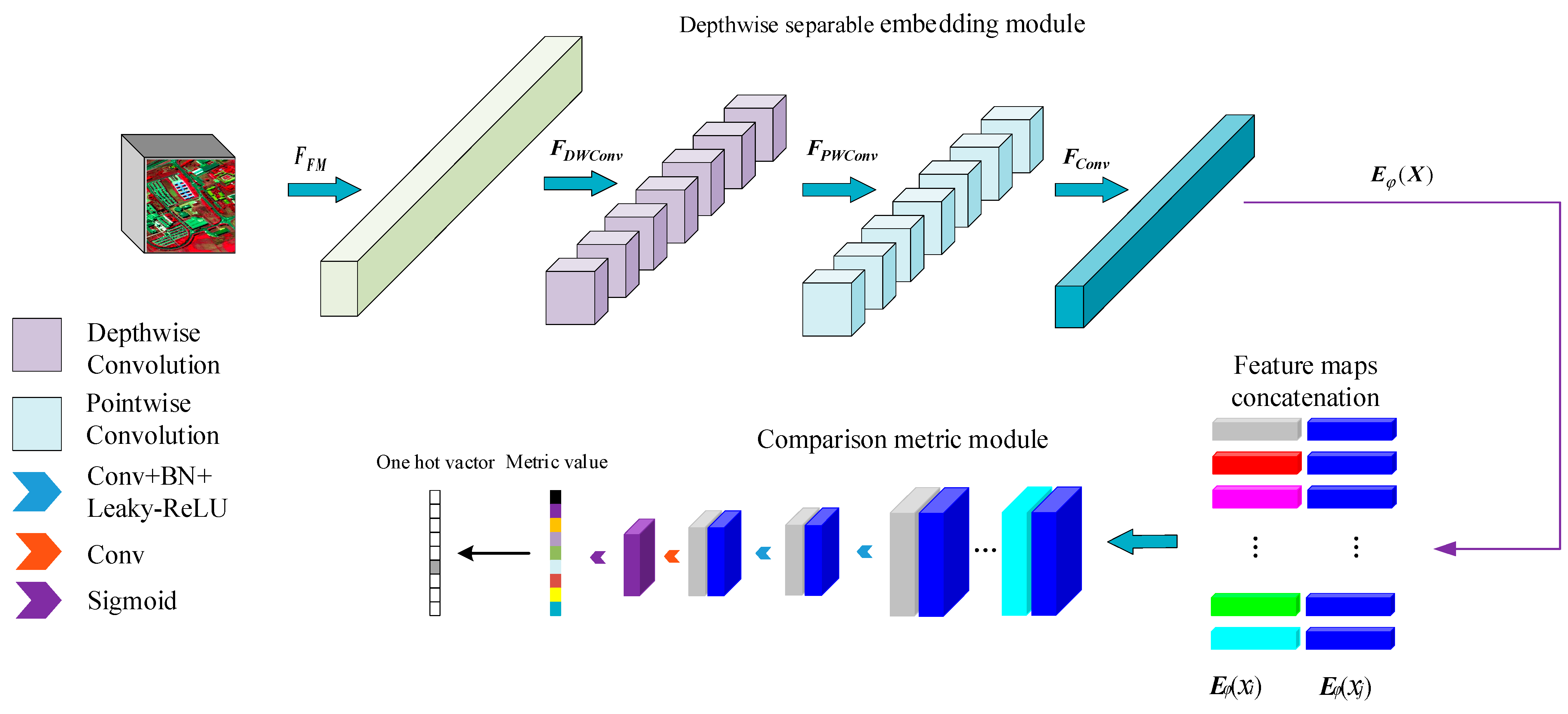
The classification model proposed in this paper is shown in Figure 1, and is composed of depthwise separable embedding model and comparison metric module. To avoid the classification model falling into local optimal solutions, the method in this paper adopts the cosine annealing algorithm to train the network model. Firstly, the samples are input into the deep separable embedding model, and the first layer of the model is used to extract the rough features of the samples. To activate the neurons more effectively, the Leaky-ReLU activation function is added to each layer of the neural network, and then the obtained features are input into the depthwise separable convolution, which can be divided into deep convolution and point-by-point convolution. Deep convolution convolutes each input channel to obtain finer spatial features. The spatial information between channels is fused by point-by-point convolution to preserve the interaction between channels. The feature vectors output by the embedded model are input into the relation model. The feature vectors of support samples and query samples are symmetrically spliced one by one. The spliced feature vectors are regarded as sample pairs with symmetrical structure, and then the sample pairs are mapped to the comparative metric model to obtain the measurement distance between symmetrical structures. The matching degree between samples is analyzed by neural network, and finally the terrain category is obtained.
2.1. Depthwise Separable Embedding Model
The purpose of the deep separable embedding model is to obtain high-quality feature vectors, so as to splice high-quality symmetric feature spaces with comparative metric models. In deep learning, convolutional neural network is widely used in the field of image classification because of its strong feature expression ability [34]. The convolutional neural network obtains the information of different feature maps at different positions through neurons, so that the obtained images have richer features. With the deepening of the number of network layers, the convolutional neural network can deal with more complex actual environments; however, it also faces some problems, such as increasing computational cost, difficult convergence of the network, and much dependence on samples [35]. Therefore, on the basis of the premise that the convolutional neural network can obtain richer images, this paper introduces the lightweight depthwise separable convolutional network model to reduce the network model parameters and improve the model training speed, and introduces the Leaky-ReLU activation function to effectively activate the neurons in each layer of neural network and increase the processing ability of the model to complex environment.
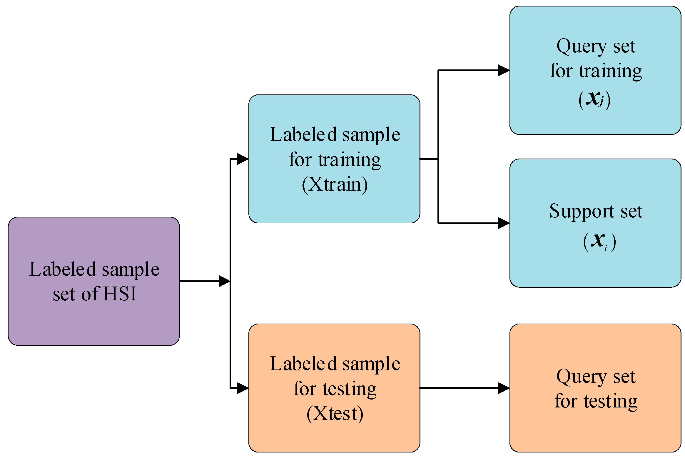
In each training process, the sample is defined as , the training sample is defined as , and the embedded feature is defined as , where is the total number of training samples, and the training samples are divided into query samples and support samples , which have corresponding tag values and . Each time, one query sample and several support samples are randomly selected from the training set to train the model. The query sample is the sample to be classified, and each supporting sample represents its own category information. In the same way as to construct the samples of , query samples are randomly selected from , as shown in Figure 2.
Firstly, the training samples are input into the first layer of convolution, and the rough features are extracted from the samples to generate a 64-channel feature map, in which represents the standard convolution operation and represents the extracted feature mapping from . Then, a depthwise separable convolutional pair is used for to complete nonlinear mapping, as shown in Formula (1).
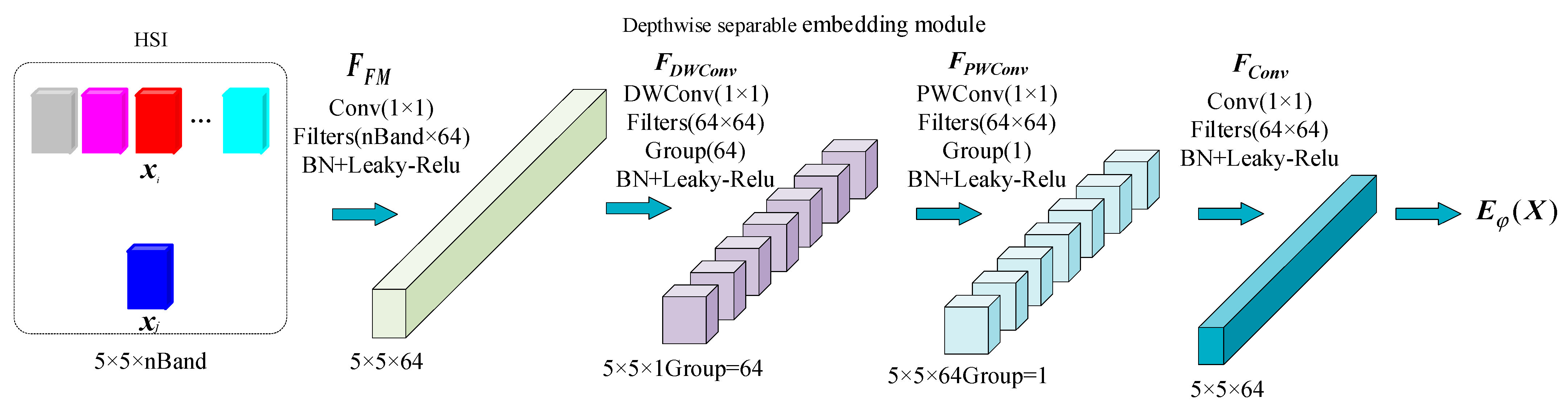
Depthwise separable convolution (DS) can be divided into depthwise convolution (DW) and pointwise convolution (PW). DW convolutes each independent channel to obtain finer spatial features . The depthwise separable embedding model is shown in Figure 3. Because a feature map (FM) is convoluted by only one filter, the feature information of different channels at the same spatial position cannot be effectively used. Therefore, pointwise convolution is introduced to fuse the spatial information between the same positions and preserve the interactivity of the channel to obtain the spatial feature , and then the sample feature vector is obtained from the convolution layer , as shown in Formula (2).
Figure 3 shows the output of each layer of depth separable embedding model. In this paper, the depth separable embedding model consists of three layers of neural network. The first and third layers are composed of conventional convolution layer, batch normalization layer (BN) and Leaky-ReLU activation function. The second layer is the depthwise separable convolution layer, including depthwise convolution and pointwise convolution. The depthwise convolution is composed of 64 groups of convolution layer, BN layer and Leaky-ReLU activation function. The pointwise convolution is composed of one group of convolution layer, BN layer and Leaky-ReLU activation function. To train small samples more effectively, the convolution core size of each layer of neural network is set to , where padding is 0 and stripe is 1. Assuming the input sample is , after the first layer of convolution, the feature map has a size of . The second layer of depthwise separable convolution is further filtered to generate 64 groups of isolated feature map, then one group with a size of is generated by to fuse the information of different feature maps, and finally the conventional convolution output has a size of .
2.1.1. Depthwise Separable Convolution
Hyperspectral images are different from general two-dimensional images, and contain a lot of information in the spatial dimension. The spatial information of hyperspectral images determines the spatial features between adjacent pixels in the spatial dimension, and the spatial features can make up for the shortcomings of spectral domain features to improve the ability of model to capture features. Although the two-dimensional convolution neural network can also extract the spatial features of hyperspectral images, it is not conducive to extracting the spectral and spatial features of pixels at the same time. In view of the insufficient use of hyperspectral data information by two-dimensional convolution, a depthwise separable convolution layer is added after the two-dimensional convolution layer, which can reduce the parameters and increase the spatial features at the same time [36]. More abundant spatial–spectral features are extracted to ensure that the model can distinguish the spatial information of different bands without loss.
The two-dimensional convolution generates new high-level features through the filtering features and merging features of the convolution kernel. Each channel of the convolution layer can be expressed as Formula (3), where is the channel of the convolution feature graph, represents the convolution kernel, is the offset term of the feature graph, and is the channel of the previous layer. The operator represents the two-dimensional convolution operation and represents the nonlinear Leaky-ReLU activation function to speed up the training process of network model.
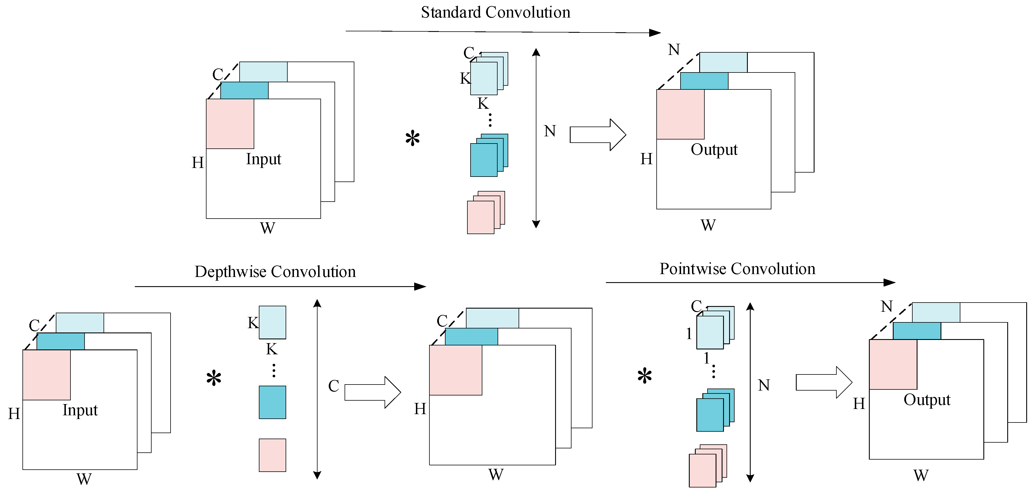
Formula (4) represents the calculation amount of standard convolution operation. The size of the output feature map is defined as , the number of channels is , the size of the convolution kernel is , the number of convolution kernels is , and the feature map is convoluted with each convolution kernel.
The depthwise separable convolution performs a single channel filtering operation for each input channel, added after the depthwise convolution filtering, and performs pointwise convolution. It is assumed that the input samples have a depth convolution size of and are divided into groups, then, each group performs conventional convolution, which is equivalent to extracting the spatial features of each input channel , that is, the features of DW, and the output is size of . The features of each sample point after pointwise convolution have a size of , i.e., the features of PW, and the output is size of . Formula (5) represents depth convolution and Formula (6) represents point-by-point convolution. The structure of depthwise separable convolution is shown in Figure 4, where is convolution operation.
Because the convolution neural networks of the second and third layers are processed together after the depthwise separable convolution is introduced, the parameters of the depthwise separable convolution are compared with those of the second and third layers and the two-layer convolution layer. Therefore, the parameter quantity in this paper is compared with the two-layer convolution neural network shown as follows:
2.1.2. Leaky-ReLU Activation Function
In the multilayer neural network, each neuron node accepts the output value of the upper neuron as the input value of the neuron, and transmits the input value to the next layer. The output of the upper node and the input of the lower node are transmitted through the activation function. To ensure that the neuron adapts to the complex linear relationship, the ReLU activation function is generally added to the neural network. The ReLU activation function refers to the modified linear unit. Only when the input value is positive will the neuron will be effectively activated, causing the model to lose part of the characteristic information in the negative signal. However, when the input is negative, the learning speed of the ReLU activation function becomes very slow, even directly making the neuron invalid. At this time, the input is negative, and the gradient is zero, so its weight cannot be updated. The mathematical expression of ReLU function is:
Therefore, a linear element function with leakage correction is introduced, namely the Leaky-ReLU function. The function introduces a leakage value in the negative value interval of the ReLU function, and has a small slope for the negative value input, so that the derivative is always non-zero, reducing the emergence of silent neurons and effectively activating neurons in the network. The mathematical expression of the Leaky-ReLU function is:
where , and a small slope is given, that is, the negative input information is retained without increasing the computational cost of model training. is the input. On the one hand, it modifies the data distribution, on the other hand, it weights the negative value data with constant to retain the input information more completely. Compared with the ordinary ReLU function, Leaky-ReLU keeps the features of HSI negative signal data through a very small negative value weighting constant. After the Leaky-ReLU replaces the ReLU activation function and is nonlinearly weighted to the output of each convolution and full connection layer, when the input signal gradient is input to the Leaky-ReLU activation function and the input signal is less than 0, the output is a linearly weighted input signal . When it is greater than zero, the output is equal to the input.
2.2. Cosine Annealing Algorithm
The gradient descent method is an iterative algorithm that solves the gradient vector of the objective function, updates the parameter value along the direction of negative gradient, and solves the minimum of the objective function until convergence. Therefore, it is necessary to set , and then update each parameter of the network along the negative gradient direction to minimize the loss function. Generally, in deep learning, batch gradient descent (BGD) and stochastic gradient descent (SGD) are mainly used to update the parameter values. BGD needs to use all datasets to update each parameter. If the number of samples is too large, the training speed will be too slow, and the calculation cost will be increased. Although SGD has the characteristics of fast training speed, it is easy to fall into the local optimal solution because it only uses part of the information in the data. Therefore, on the premise of integrating the training sample speed and calculation cost, this paper introduces the cosine annealing algorithm to update the parameter value, which can reduce the learning rate through the cosine function, as shown in the following:
where and are the minimum and maximum learning rate respectively, is the total number of epochs, is the current epoch. usually decays. When , reaches the minimum training batch.
2.3. Comparison Metric Model
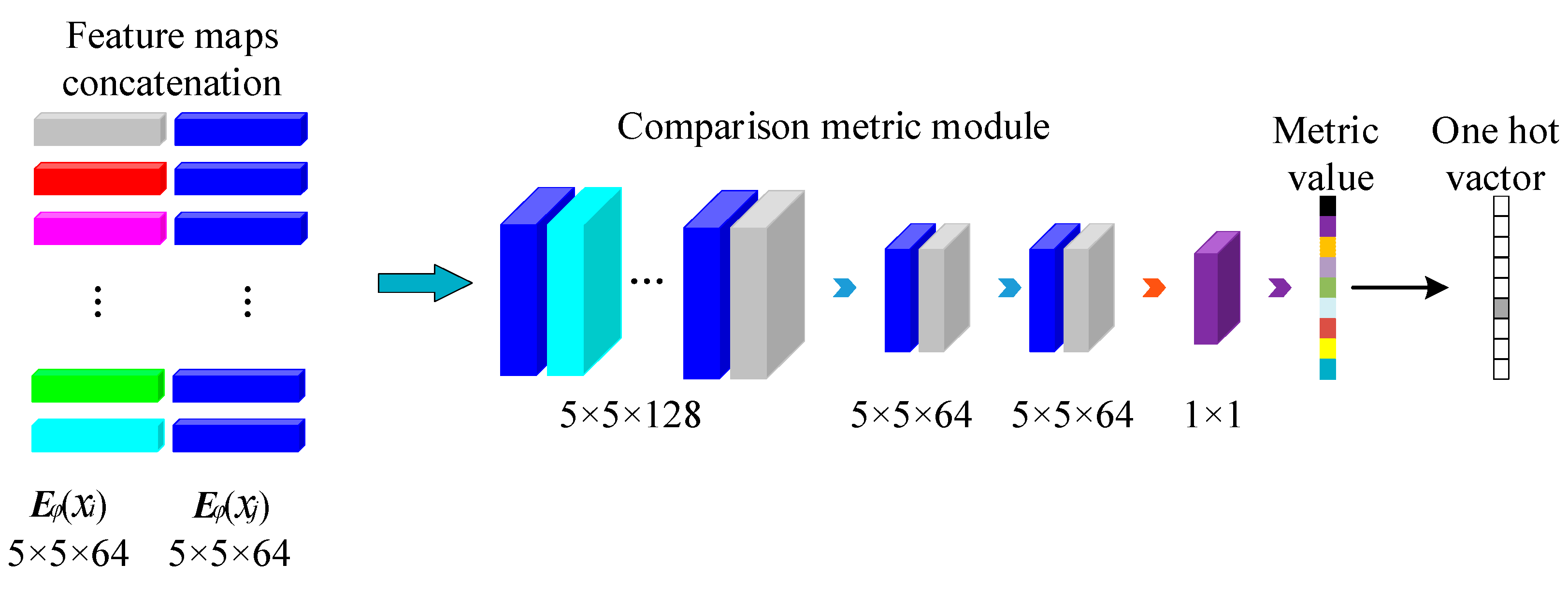
It is known that the support samples and query samples generate the sum of two sets of feature vectors and size of through the depth separable embedding model, and a feature vector with size is generated after symmetric splicing operation , as shown in Formula (11). If the number is equal between and , the symmetric splicing operation recombines the unevenly distributed and and one-to-one splices to form a feature space with symmetric structure. Each time, a group of samples is mapped onto the comparative metric model. By measuring the metric distance between the symmetric structures of the samples, a small number of features can be effectively used to obtain the attributes of samples and reduce the dependence of the model on training samples.
is a neural network composed of three convolution layers. The convolution size of the first two layers is . After the first two convolution layers, the Leaky-ReLU activation function is used for nonlinear feature mapping. The third convolution layer has a size of , and then the sigmoid function is used to output a specified scale to describe the similarity between samples, which is shown in Formula (12), and the value range of the function is .
Then, the output feature vector is mapped to , and the distance between the eigenvector and is measured by a convolution layer size of . The feature vector with size is generated, and a relationship score with size is generated by to analyze the similarity between samples. Finally, is compared with , which is the class with the highest relationship score. The comparison metric model is shown in Figure 5.
To determine the label of the query sample, the feature map of each combination is put into to generate a similarity, whose definition is as shown in Equation (13) to represent the similarity between any two embeddings. The output value is in the range , which is considered that the score of similar relationship. The higher the output value, the greater the similarity.
The comparison metric model is trained by calculating the relationship scores between and by using the minimum mean square error (MSE) loss function. The loss function is represented by Formula (14), where refers to when the training sample belongs to the same category and , in which case it is 1, otherwise it is 0.
3. Experimental Results and Analysis
3.1. Hyperspecral Dataset Description
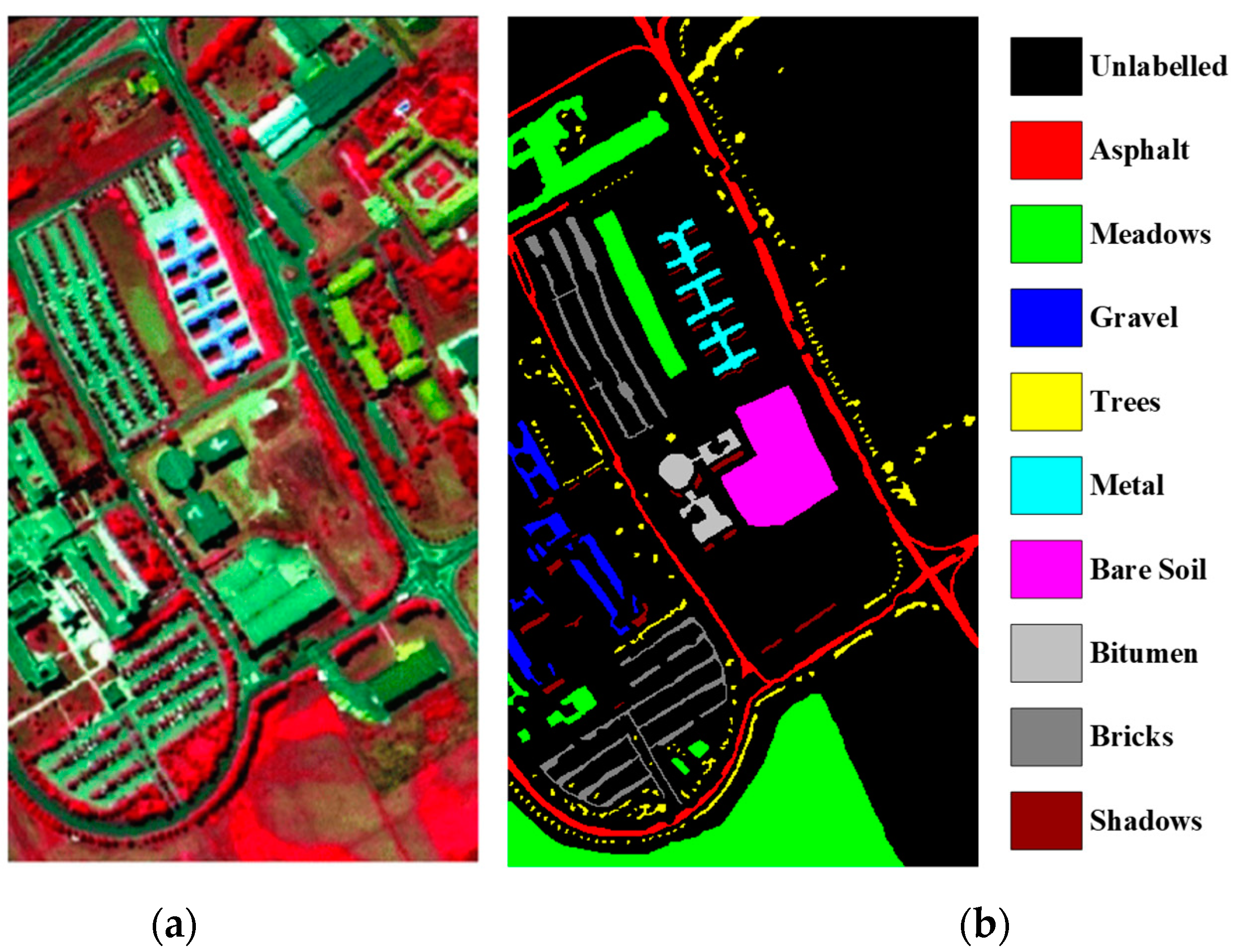
To verify the effectiveness of the proposed model for hyperspectral data classification, this paper uses two public hyperspectral datasets, the Pavia University (PaviaU) dataset and the KSC dataset. The Pavia University dataset is an urban scene collected from hyperspectral images of Pavia University in Italy in 1992, including multiple types of urban features. The image size is pixels with a spatial resolution of 1.3 m, including 103 spectral bands after denoising (band range from 0.43 to 0.86 μm), a total of nine classes and 42,776 labeled samples were calibrated, as shown in Figure 6.
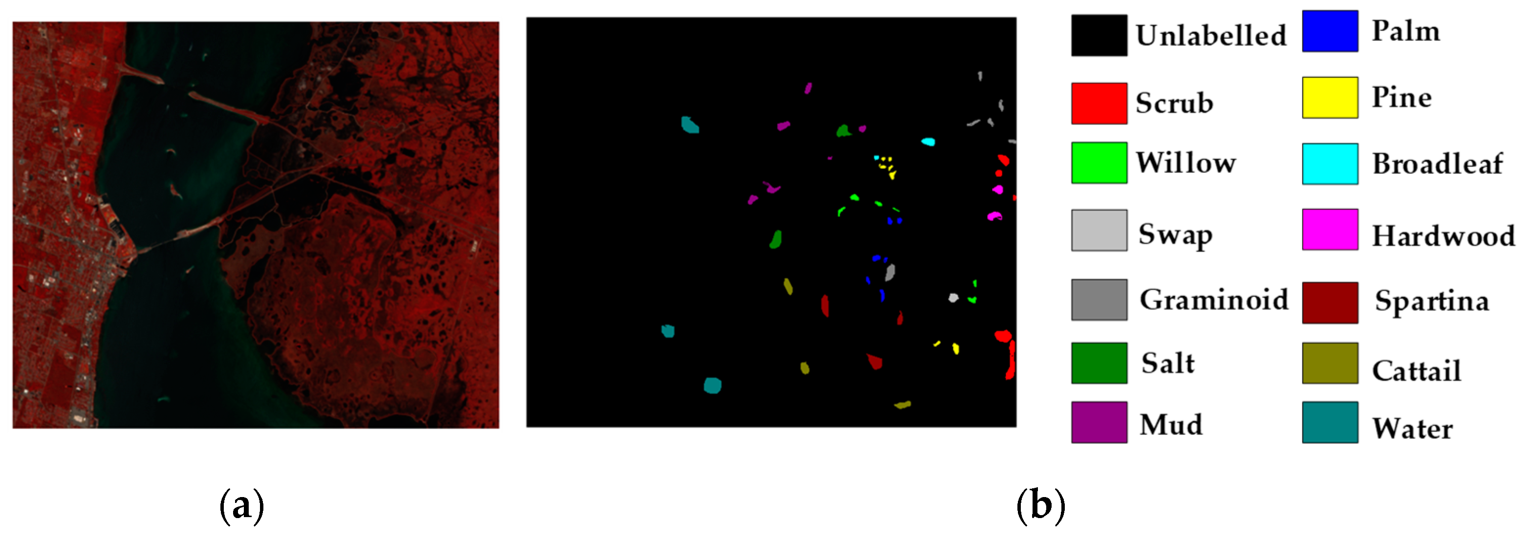
The KSC dataset was collected from mixed vegetation near Kennedy Space Center by the airborne visible/infrared imaging spectrometer (AVIRIS) of the National Aeronautics and Space Administration (NASA) on 23 March, 1996. The image size is pixels with a spatial resolution of 18 m. Some atmospheric water absorption bands and low signal-to-noise ratio (SNR) bands were discarded, and only 176 bands were reserved for analysis. A total of 13 categories and 5211 labeled samples were calibrated, as shown in Figure 7 [37].
3.2. Experimental Platform Parameter Settings
In this paper, Windows 7 was used as the operating system. The experimental environment was Intel (R) core (TM) i5-6500 CPU @ 3.2 GHz processor, 16 GB running memory (RAM), NVIDIA GeForce GTX 1060 GPU. In addition, the deep learning framework was Pytorch, which uses Python as the programming language. To obtain more stable statistics data, all the experimental results presented in this paper are the average of 10 experiments. In the network training part, all experiments adopt a batch processing method. Because reducing the parameters in the network is conducive to small sample training, the size of the input data was set to 5, the number of training epochs was set to 4000, the momentum was set to 1 and the learning rate of cosine annealing was set to 0.1.
To ensure the reliability of the experiment, the training samples of all experiments were randomly selected from hyperspectral data. In addition, eight different methods were used to evaluate the performance of the proposed relational network for comparison, including morphological contour support vector machine (EMP-SVM), deep convolution neural network (DCNN), deep residual network (ResNet), pyramid residual network (PyResNet), relational network (RLNet), relational network based on depthwise separable convolution (DRNet), Leaky-ReLu relational network (LRNet)) and deep separable Leaky-ReLu relational network (DLRNet).
The evaluation indexes of classification results in the experiments adopted the overall accuracy (OA), average accuracy (AA) and Kappa coefficient (K) commonly used in remote sensing data classification. OA is the proportion of the number of correctly classified samples to the total number of samples, which measures the overall classification effect. AA is the mean of each class’s accuracy, which can better measure the classification effect of small sample categories. Kappa coefficient can not only measure the classification accuracy, but also measures the consistency between the model prediction effect and the actual effect.
3.3. Design of Relation Network Model
In this paper, the neural network with depthwise separable convolution is introduced as the feature extraction network of the embedded model. The network is composed of a convolution layer, a depthwise separable convolution layer, the Leaky-ReLU activation function and a normalization layer. To train small amounts of sample data more fully, the lightweight depthwise separable convolution network model is introduced, which not only saves the computational cost, but also improves the training efficiency of the model. The Leaky-ReLU activation function is introduced to further accelerate the convergence speed and reduce the emergence of silent neurons. Because hyperspectral data have rich spectral information and spatial information, each hyperspectral pixel and its band number (nband) are set as the input, and the model input size is . Since the model is trained on a small number of labeled samples, reducing the parameters in the network is more conducive to training; therefore, the size of convolution kernel in neural network is set as . At the same time, the number of filters per layer is set to 64, and the final output is . The relational model contains three conventional convolution layers and convolution kernel, the Leaky-ReLU activation function, two BN layers and one Sigmoid layer. Table 1 shows the parameter settings of the depthwise separable embedding model.
3.4. Comparison of Experimental Results
In this section, the OA, AA and kappa coefficients are compared and analyzed on two public HSI datasets. It can be found from Table 2 and Table 3 that the proposed algorithm in this paper is superior to other classification methods. Comparing DLRNet to RLNet, it can be found that the performance of DLRNet is better than the latter. The introduction of depthwise separable convolution reduces the parameters of the model, reduces the dependence of the model on computational power, and improves the universality of the model. At the same time, the Leaky-ReLU activation function is introduced to add a leakage value so that the neurons of the network model can be activated effectively. To avoid the model falling into local optimal solutions, the network model is trained by the cosine annealing algorithm. Therefore, compared with other classification methods, the model in this paper has excellent classification accuracy.
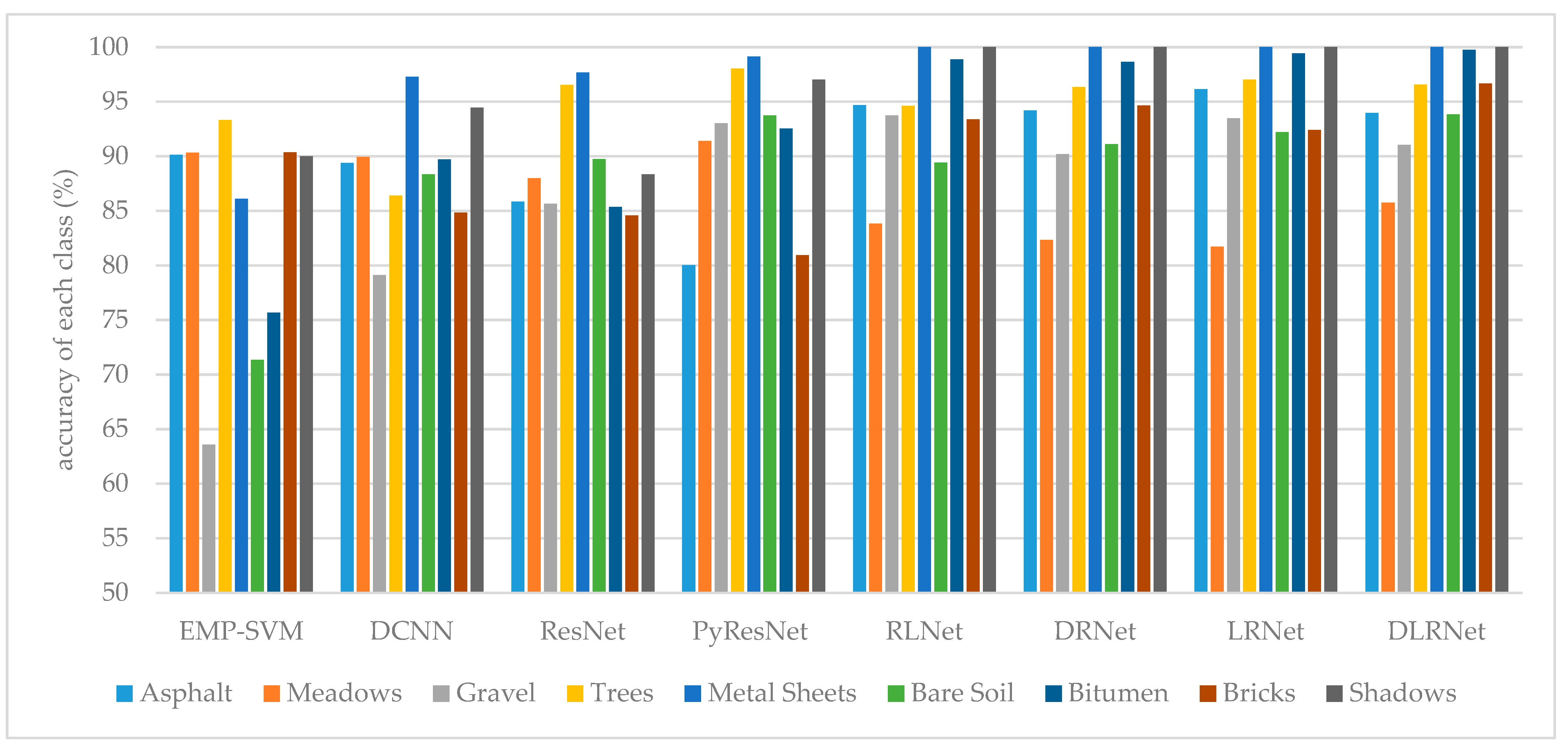
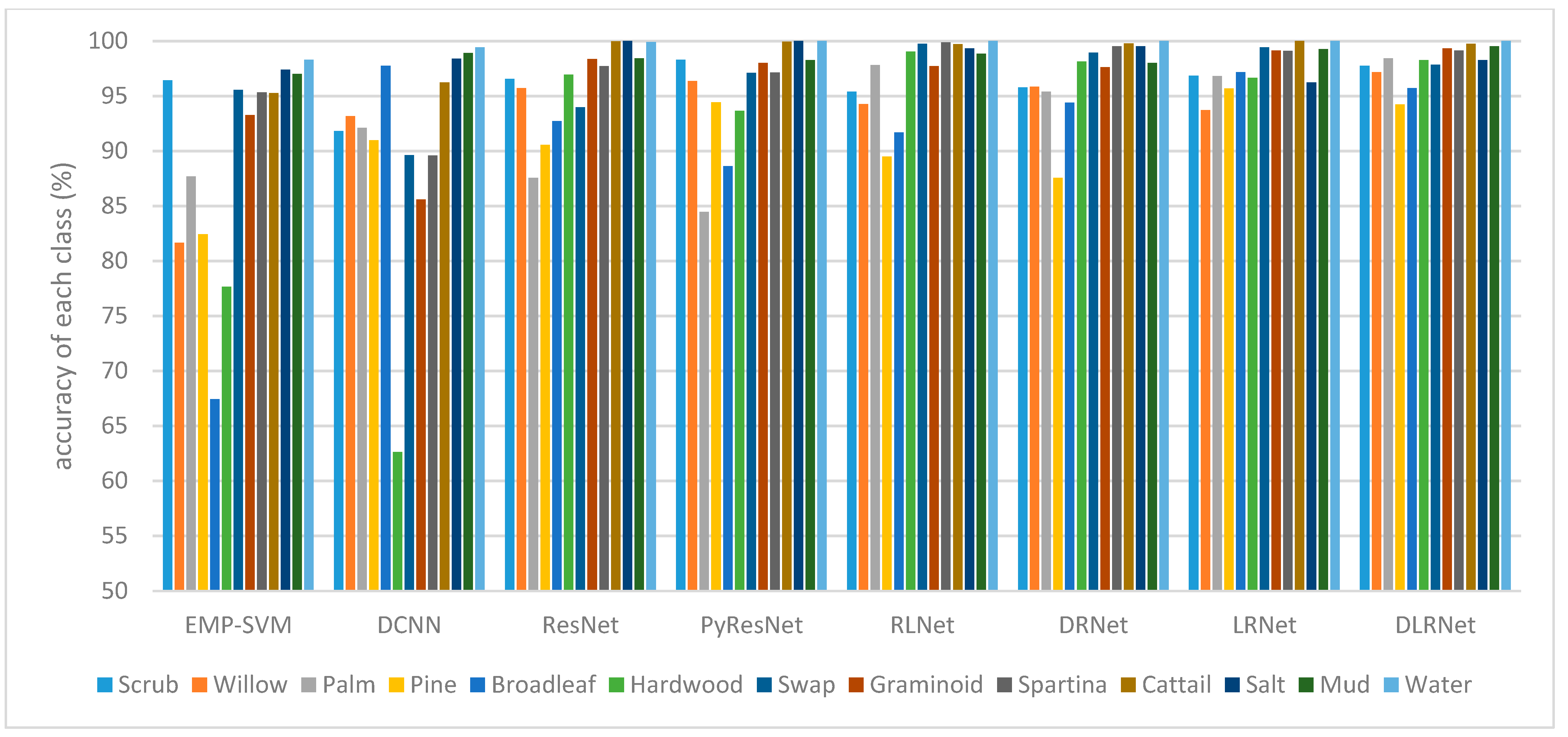
It can be seen from Table 2 that the highest OA on PaviaU dataset is 91.12%, which is an increase of 2.16%, 1.48%, 0.8%, 0.22%, 1.56%, 2.05% and 1.84%, respectively, compared with EMP-SVM, DCNN, ResNet, PyResNet, RLNet, DRNet and LRNet. It can be seen from Table 3 that the highest OA obtained by this classification model on the KSC dataset is 98.61%, which is an increase of 6.4%, 5.6%, 1.82%, 1.68%, 0.83%, 0.99% and 0.49%, respectively, compared with EMP-SVM, DCNN, ResNet, PyResNet, RLNet, DRNet, and LRNet, which fully proves the effectiveness of DLRNet model hyperspectral data classification with small samples. Figure 8 and Figure 9 show the classification results of different methods for each class on the PaviaU and KSC datasets, respectively.
The running time of the model is an important evaluation index of the deep learning classification model. Table 4 shows the calculation time of the eight network models. By comparing DLRNet and RLNet, it can be found that the training efficiency of the network model is improved, and it is reduced by 0.47 min and 0.49 min in the PaviaU dataset and KSC dataset, respectively, by introducing depthwise separable revolution and Leaky-ReLU, which proves the effectiveness of the method proposed in this paper. Although DLRNet consumes a large amount of time compared with EMP-SVM and DCNN, these traditional algorithms rely too much on the number of samples, which is not conducive to the classification of the real environment. Compared with the difficulty of obtaining labeled samples, the increase of time is acceptable.
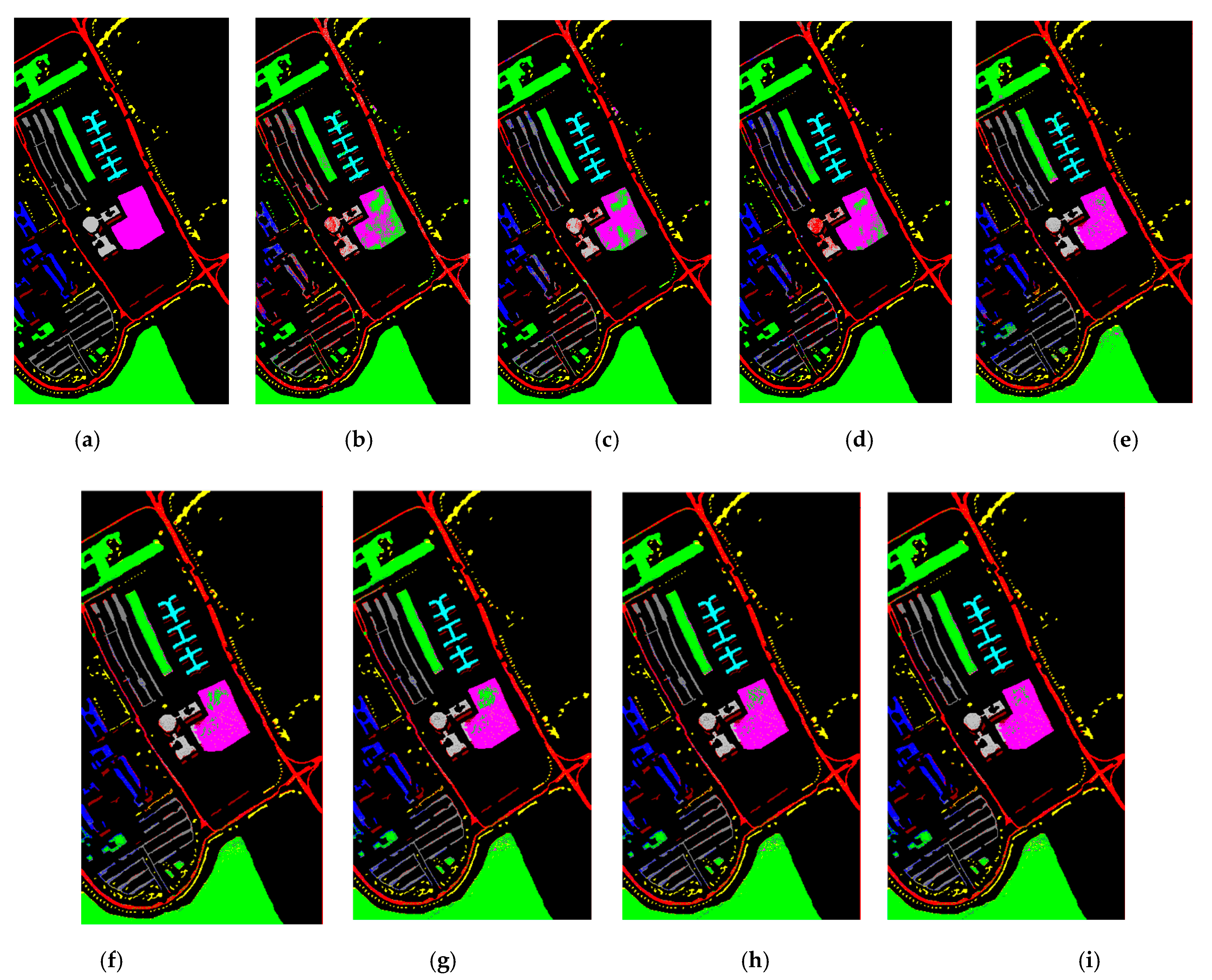
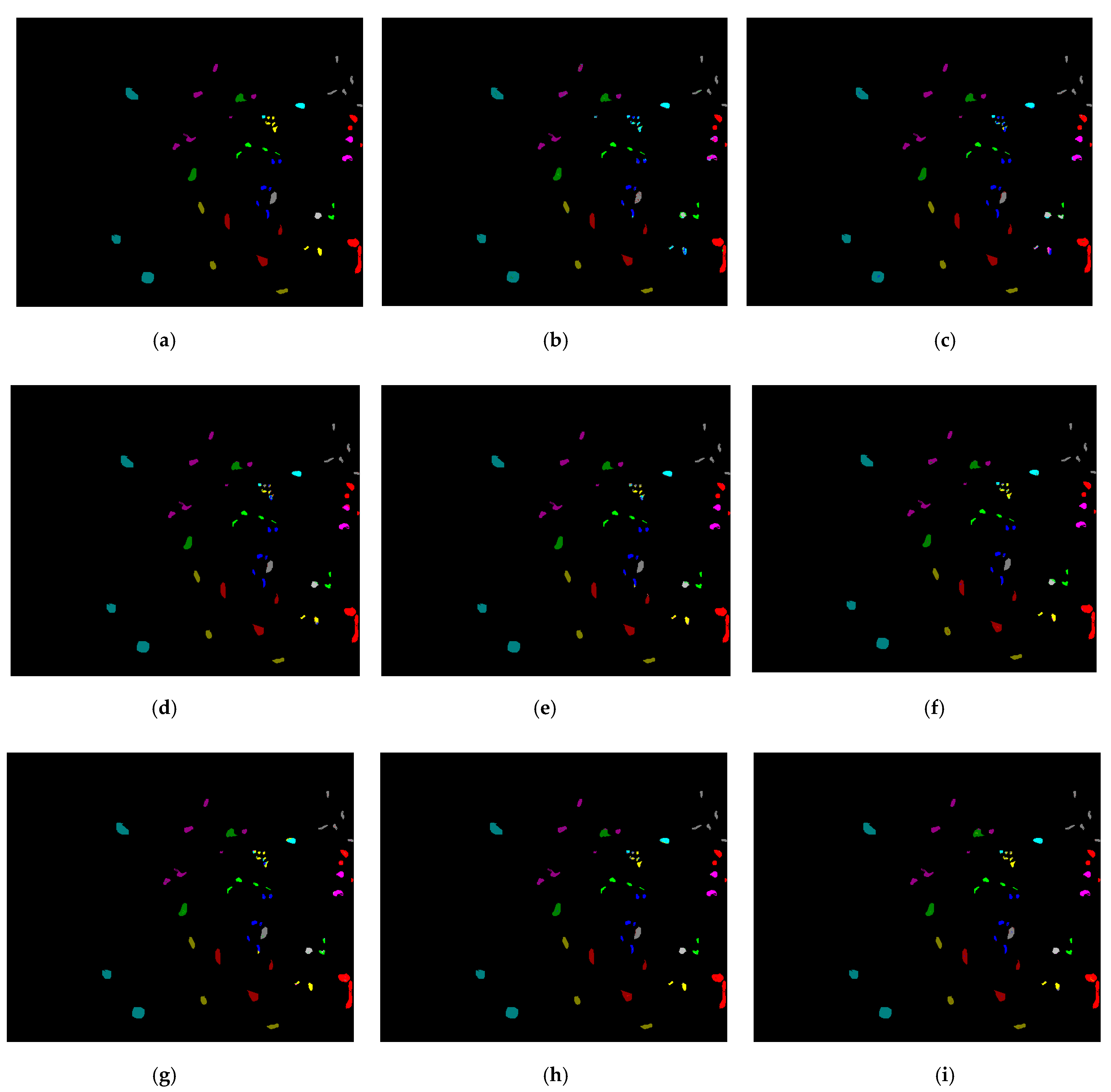
To subjectively evaluate the classification effects, Figure 10 and Figure 11 show the ground truth of two HSI data and the pseudo color maps of the classification results of each method, respectively. It can be seen that the classification results obtained by our method are closer to the distribution of real terrain, and the area of false classification is greatly reduced. Compared with seven other methods, the classification accuracy is greatly improved.
4. Discussion
4.1. The Selection of Small Sample Number
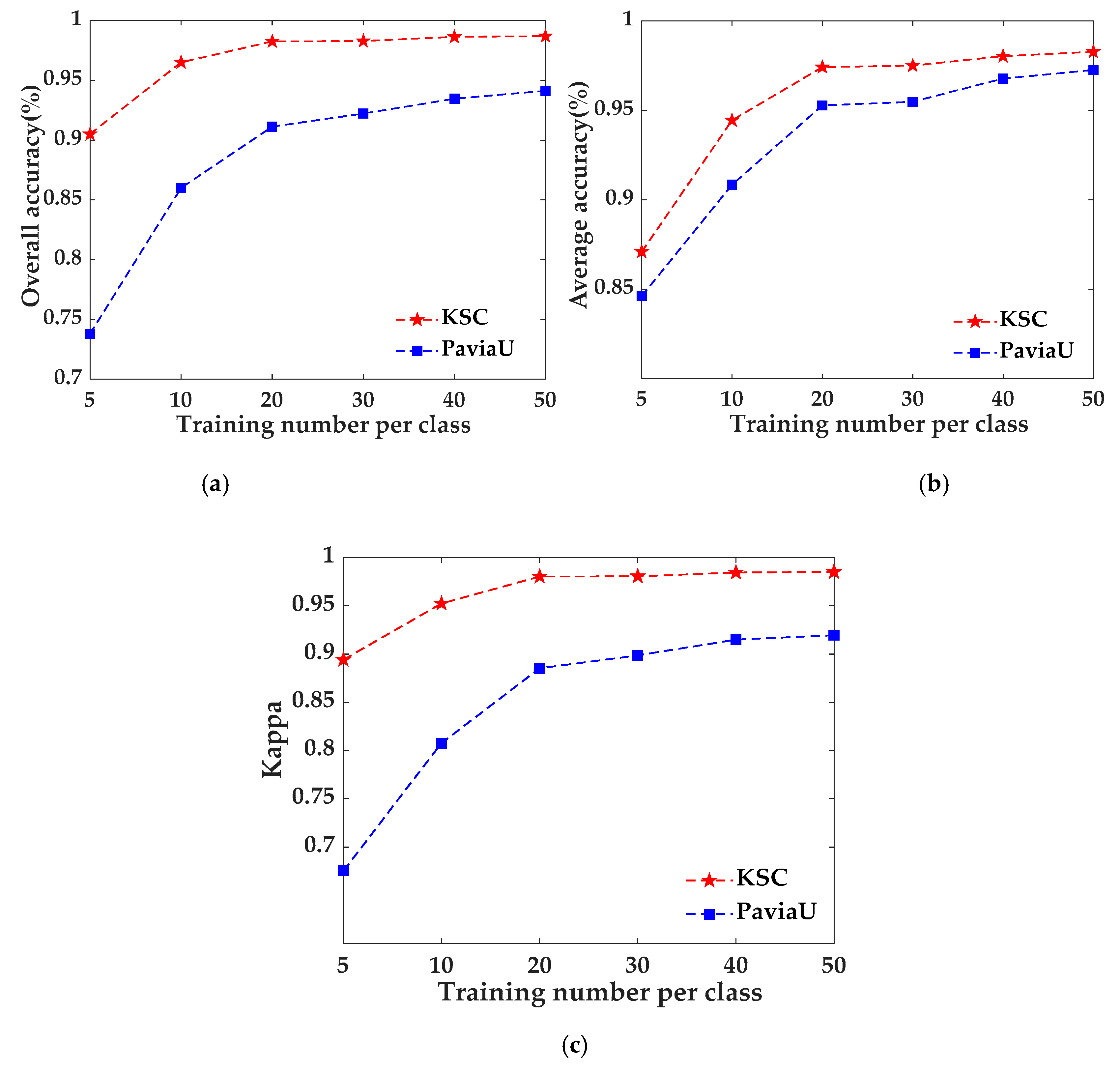
The number of small samples is defined as the number of samples of each class, which is selected as 5, 10, 20, 30 and 40. Comparing the five sample sizes, it can be found in Figure 12 that when the sample number of each class is 20, the growth of OA reaches its peak and is relatively slow after 20. Therefore, this paper sets the number of training samples of each class to 20.
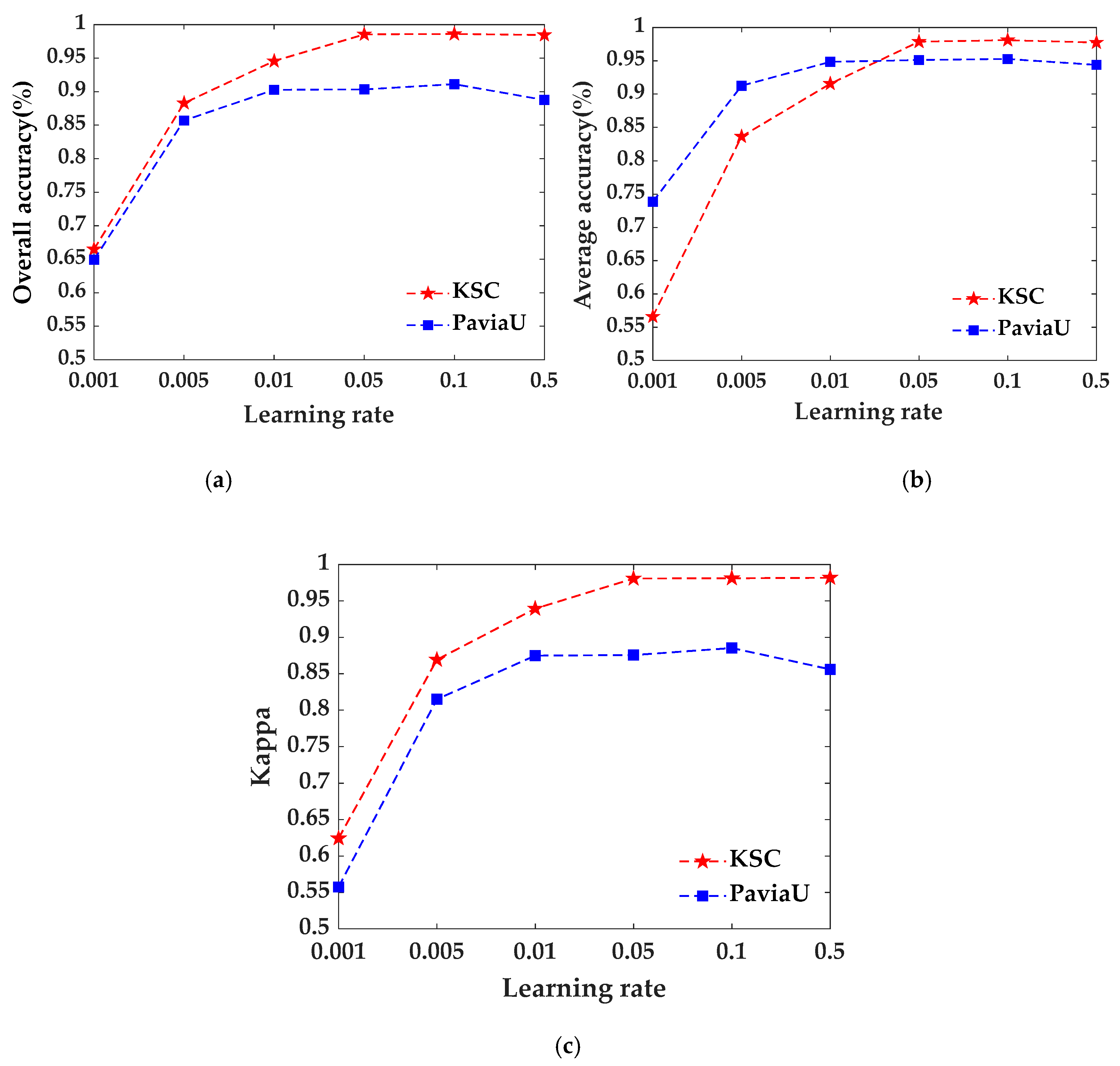
4.2. The Selection of Learning Rate
To better verify the influence of cosine annealing algorithm on the proposed model, this paper compares experimental results with different learning rates of 0.5, 0.1, 0.01, 0.05, 0.001 and 0.005. Figure 13 shows the values of OA, AA and Kappa corresponding to different learning rates on the two datasets. It can be found that although the learning rate can be changed automatically by using cosine degradation algorithm, the selected learning rate should not be too large. When the learning rate is 0.1, OA, AA and Kappa reach their optimum levels, and when the learning rate is 0.5, the values of OA, AA and Kappa are reduced. Therefore, this paper sets the learning rate as 0.1.
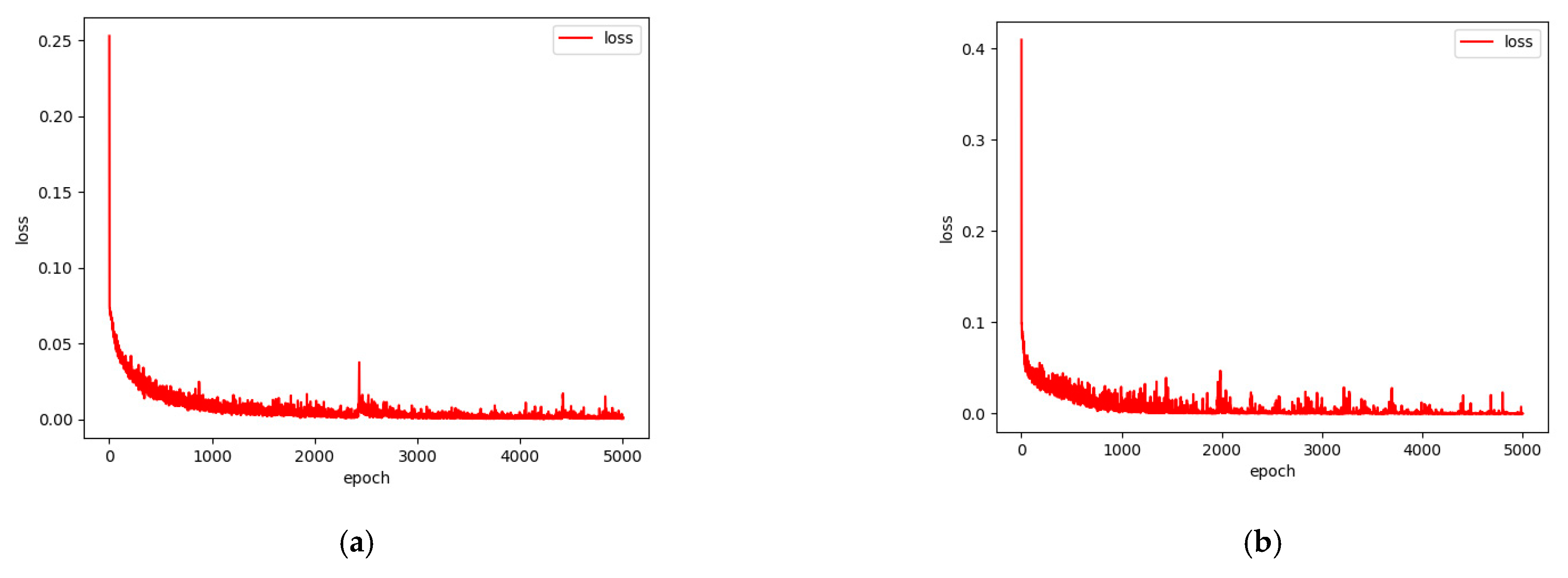
Figure 14 shows the loss of the network corresponding to the two datasets in the training phase. With the increase of the number of epochs, the loss continues to decrease. We can see that the corresponding networks on the two datasets basically reach the convergence state when the epoch is about 4000. Therefore, it is verified that the network model in this paper converges easily.
4.3. Comparison of Parameters between Different Classification Models
To better describe the reduced parameters of depthwise separable convolution, this paper compares it with the ordinary four-layer convolution neural network, as shown in Table 5. The convolution neural networks of the second and third layers are processed together after the depthwise separable convolution is introduced. As shown in Table 5, the sum parameter number of Conv-1 and Conv-2 is 8320 for CNN, while the number of DSConv-2 is 4288, meaning that the parameters of the depthwise separable convolution are reduced by 48.46% compared with the two-layer ordinary convolution. The parameters of the overall four-layer embedding model of the PaviaU and KSC models were reduced by 20% and 16.58%, respectively. Compared with ordinary convolution, depthwise separable convolution has fewer parameters and better performance.
5. Conclusions
In this paper, a hyperspectral image classification algorithm based on a depthwise separable relational network is proposed for small sample classification. The depthwise separable convolution is introduced into the deep embedding model to improve the training efficiency of the model. In addition, a learning rate adjustment strategy effectively reduces the time required to improve the classification performance of the model and improve the classification accuracy of the model. We have carried out experiments on two public HSI datasets, and compared DLRNet with other seven methods to verify the effectiveness of the proposed method. The experimental results show that our proposed method is more competitive. Its OA on the PaviaU dataset and the KSC dataset reaches 91.12% and 98.61%, respectively, which is better than other classical methods and ordinary relational network methods and implies that our proposed model could be a promising research direction for solving the limited training sample problem, especially in the context of HSI classification.
Author Contributions
Conceptualization, A.W. and H.W.; methodology, C.L.; software, C.L. and D.X.; validation, Y.Z. and M.L.; writing—review and editing, C.L. and A.W.; All authors have read and agreed to the published version of the manuscript.
Funding
This work was funded by the National Natural Science Foundation of China under Grant NSFC-61671190.
Institutional Review Board Statement
Not applicable.
Informed Consent Statement
Not applicable.
Data Availability Statement
The data are available at http://www.ehu.eus/ccwintco/index.php?title=Hyperspectral_Remote_Sensing_Scenes (accessed on 10 August 2021).
Acknowledgments
We thank for Kaiyuan Jiang and Lanfei Zhao for their valuable comments and discussion.
Conflicts of Interest
The authors declare no conflict of interest.
References
- Camps-Valls, G.; Tuia, D.; Bruzzone, L.; Benediktsson, J.A. Advances in hyperspectral image classification: Earth moni-toring with statistical learning methods. IEEE Signal Process. Mag. Jan. 2014, 31, 45–54. [Google Scholar] [CrossRef] [Green Version]
- Zhang, C.; Kovacs, J.M. The application of small unmanned aerial systems for precision agriculture: A review. Precis. Agric. 2012, 13, 693–712. [Google Scholar] [CrossRef]
- Atkinson, J.T.; Ismail, R.; Robertson, M.P. Mapping Bugweed (Solanum mauritianum) Infestations in Pinus patula Plantations Using Hyperspectral Imagery and Support Vector Machines. IEEE J. Sel. Top. Appl. Earth Obs. Remote Sens. 2013, 7, 17–28. [Google Scholar] [CrossRef]
- Bioucas-Dias, J.M.; Plaza, A.; Camps-Valls, G.; Scheunders, P.; Nasrabadi, N.; Chanussot, J. Hyperspectral Remote Sensing Data Analysis and Future Challenges. IEEE Geosci. Remote Sens. Mag. 2013, 1, 6–36. [Google Scholar] [CrossRef] [Green Version]
- Wang, Z.; Du, B.; Shi, Q.; Tu, W. Domain Adaptation with Discriminative Distribution and Manifold Embedding for Hy-perspectral Image Classification. IEEE Geosci. Remote Sens. Lett. 2019, 16, 1155–1159. [Google Scholar] [CrossRef]
- Melgani, F.; Bruzzone, L. Classification of hyperspectral remote sensing images with support vector machines. IEEE Trans. Geosci. Remote Sens. 2004, 42, 1778–1790. [Google Scholar] [CrossRef] [Green Version]
- Chen, Y.; Nasrabadi, N.M.; Tran, T.D. Hyperspectral Image Classification Using Dictionary-Based Sparse Representation. IEEE Trans. Geosci. Remote Sens. 2011, 49, 3973–3985. [Google Scholar] [CrossRef]
- Gislason, P.O.; Benediktsson, J.A.; Sveinsson, J.R. Random Forests for land cover classification. Pattern Recognit. Lett. 2006, 27, 294–300. [Google Scholar] [CrossRef]
- Bandos, T.V.; Bruzzone, L.; Camps-Valls, G. Classification of Hyperspectral Images with Regularized Linear Discriminant Analysis. IEEE Trans. Geosci. Remote Sens. 2009, 47, 862–873. [Google Scholar] [CrossRef]
- Bachmann, C.; Ainsworth, T.; Fusina, R. Exploiting manifold geometry in hyperspectral imagery. IEEE Trans. Geosci. Remote Sens. 2005, 43, 441–454. [Google Scholar] [CrossRef]
- Mianji, F.A.; Zhang, Y. Robust Hyperspectral Classification Using Relevance Vector Machine. IEEE Trans. Geosci. Remote Sens. 2011, 49, 2100–2112. [Google Scholar] [CrossRef]
- Huang, X.; Guan, X.; Benediktsson, J.A.; Zhang, L.; Li, J.; Plaza, A.; Mura, M.D. Multiple Morphological Profiles from Multicomponent-Base Images for Hyperspectral Image Classification. IEEE J. Sel. Top. Appl. Earth Obs. Remote Sens. 2014, 7, 4653–4669. [Google Scholar] [CrossRef]
- Gu, Y.; Liu, T.; Jia, X.; Benediktsson, J.A.; Chanussot, J. Nonlinear Multiple Kernel Learning with Multiple-Structure-Element Extended Morphological Profiles for Hyperspectral Image Classification. IEEE Trans. Geosci. Remote Sens. 2016, 54, 3235–3247. [Google Scholar] [CrossRef]
- Mura, M.D.; Benediktsson, J.A.; Waske, B.; Bruzzone, L. Morphological Attribute Profiles for the Analysis of Very High Resolution Images. IEEE Trans. Geosci. Remote Sens. 2010, 48, 3747–3762. [Google Scholar] [CrossRef]
- Chen, Y.; Lin, Z.; Zhao, X.; Wang, G.; Gu, Y. Deep Learning-Based Classification of Hyperspectral Data. IEEE J. Sel. Top. Appl. Earth Obs. Remote Sens. 2014, 7, 2094–2107. [Google Scholar] [CrossRef]
- He, X.; Chen, Y. Optimized Input for CNN-Based Hyperspectral Image Classification Using Spatial Transformer Network. IEEE Geosci. Remote Sens. Lett. 2019, 16, 1884–1888. [Google Scholar] [CrossRef]
- Guo, A.J.X.; Zhu, F. A CNN-Based Spatial Feature Fusion Algorithm for Hyperspectral Imagery Classification. IEEE Trans. Geosci. Remote Sens. 2019, 57, 7170–7181. [Google Scholar] [CrossRef] [Green Version]
- Chen, H.; Miao, F.; Shen, X. Hyperspectral Remote Sensing Image Classification with CNN Based on Quantum Genet-ic-Optimized Sparse Representation. IEEE Access 2020, 8, 99900–99909. [Google Scholar] [CrossRef]
- He, K.; Zhang, X.; Ren, S.; Sun, J. Deep Residual Learning for Image Recognition. arXiv 2015, arXiv:1512.03385. [Google Scholar]
- Paoletti, M.E.; Haut, J.M.; Fernandez-Beltran, R.; Plaza, J.; Plaza, A.J.; Pla, F. Deep Pyramidal Residual Networks for Spectral–Spatial Hyperspectral Image Classification. IEEE Trans. Geosci. Remote Sens. 2018, 57, 740–754. [Google Scholar] [CrossRef]
- Paoletti, M.E.; Haut, J.M.; Plaza, J.; Plaza, A. Neural Ordinary Differential Equations for Hyperspectral Image Classification. IEEE Trans. Geosci. Remote Sens. 2019, 58, 1718–1734. [Google Scholar] [CrossRef]
- Li, S.; Song, W.; Fang, L.; Chen, Y.; Ghamisi, P.; Benediktsson, J.A. Deep Learning for Hyperspectral Image Classification: An Overview. IEEE Trans. Geosci. Remote Sens. 2019, 57, 6690–6709. [Google Scholar] [CrossRef] [Green Version]
- He, X.; Chen, Y.; Ghamisi, P. Heterogeneous Transfer Learning for Hyperspectral Image Classification Based on Convo-lutional Neural Network. IEEE Trans. Geosci. Remote Sens. 2020, 58, 3246–3263. [Google Scholar] [CrossRef]
- Jiang, Y.; Li, Y.; Zhang, H. Hyperspectral Image Classification Based on 3-D Separable ResNet and Transfer Learning. IEEE Geosci. Remote Sens. Lett. 2019, 16, 1949–1953. [Google Scholar] [CrossRef]
- Deng, C.; Xue, Y.; Liu, X.; Li, C.; Tao, D. Active Transfer Learning Network: A Uni-fied Deep Joint Spectral–Spatial Feature Learning Model for Hyperspectral Image Classi-fication. IEEE Trans. Geosci. Remote Sens. 2019, 57, 1741–1754. [Google Scholar] [CrossRef] [Green Version]
- Zhong, C.; Zhang, J.; Wu, S.; Zhang, Y. Cross-Scene Deep Transfer Learning with Spectral Feature Adaptation for Hyper-spectral Image Classification. IEEE J. Sel. Top. Appl. Earth Obs. Remote Sens. 2020, 13, 2861–2873. [Google Scholar] [CrossRef]
- Chen, Y.; Wang, Y.; Gu, Y.; He, X.; Ghamisi, P.; Jia, X. Deep Learning Ensemble for Hyperspectral Image Classification. IEEE J. Sel. Top. Appl. Earth Obs. Remote Sens. 2019, 12, 1882–1897. [Google Scholar] [CrossRef]
- Zhang, C.; Yue, J.; Qin, Q. Global Prototypical Network for Few-Shot Hyperspectral Image Classification. IEEE J. Sel. Top. Appl. Earth Obs. Remote Sens. 2020, 13, 4748–4759. [Google Scholar] [CrossRef]
- Hoffer, E.; Ailon, N. Deep Metric Learning Using Triplet Network. In Proceedings of the International Workshop on Similarity-Based Pattern Recognition, Berlin, Germany, 12 October 2015; pp. 84–92. [Google Scholar] [CrossRef] [Green Version]
- Sung, F.; Yang, Y.; Zhang, L.; Xiang, T.; Torr, P.H.; Hospedales, T.M. Learning to Compare: Relation Network for Few-Shot Learning. In Proceedings of the IEEE Conference on Computer Vision and Pattern Recognition, Salt Lake City, UT, USA, 1 June 2018; pp. 1199–1208. [Google Scholar] [CrossRef] [Green Version]
- Deng, B.; Jia, S.; Shi, D. Deep Metric Learning-Based Feature Embedding for Hyperspectral Image Classification. IEEE Trans. Geosci. Remote Sens. 2019, 58, 1422–1435. [Google Scholar] [CrossRef]
- Ma, X.; Ji, S.; Wang, J.; Geng, J.; Wang, H. Hyperspectral Image Classification Based on Two-Phase Relation Learning Net-work. IEEE Trans. Geosci. Remote Sens. 2019, 57, 10398–10409. [Google Scholar] [CrossRef]
- Rao, M.; Tang, P.; Zhang, Z. Spatial–Spectral Relation Network for Hyperspectral Image Classification with Limited Training Samples. IEEE J. Sel. Top. Appl. Earth Obs. Remote Sens. 2019, 12, 5086–5100. [Google Scholar] [CrossRef]
- Lv, Q.; Feng, W.; Quan, Y.; Dauphin, G.; Gao, L.; Xing, M. Enhanced-Random-Feature-Subspace-Based Ensemble CNN for the Imbalanced Hyperspectral Image Classification. IEEE J. Sel. Top. Appl. Earth Obs. Remote Sens. 2021, 14, 3988–3999. [Google Scholar] [CrossRef]
- Gao, H.; Chen, Z.; Li, C. Sandwich Convolutional Neural Network for Hyperspectral Image Classification Using Spectral Feature Enhancement. IEEE J. Sel. Top. Appl. Earth Obs. Remote Sens. 2021, 14, 3006–3015. [Google Scholar] [CrossRef]
- Zhang, R.; Zhu, F.; Liu, J.; Liu, G. Depth-Wise Separable Convolutions and Multi-Level Pooling for an Efficient Spatial CNN-Based Steganalysis. IEEE Trans. Inf. Forensics Secur. 2019, 15, 1138–1150. [Google Scholar] [CrossRef]
- Si, Y.; Gong, D.; Guo, Y.; Zhu, X.; Huang, Q.; Evans, J.; He, S.; Sun, Y. An Advanced Spectral–Spatial Classifification Framework for Hyperspectral Imagery Based on DeepLab v3+. Appl. Sci. 2021, 11, 5703. [Google Scholar] [CrossRef]
Figure 1.
The overall framework of the proposed hyperspectral image classification model.

Figure 2.
The composition of labeled samples.

Figure 3.
Depthwise separable embedding model.

Figure 4.
The structure of depthwise separable convolution, where * is convolution operation.

Figure 5.
Comparison metric module.

Figure 6.
Pavia University dataset. (a) False color map; (b) ground truth map.

Figure 7.
KSC dataset. (a) False color map; (b) ground truth map.

Figure 8.
Classification results of different methods for each class on Pavia University dataset.

Figure 9.
Classification results of different methods for each class on the KSC dataset.

Figure 10.
Classification results of Pavia University dataset. (a) Ground truth; (b) EMP-SVM; (c) DCNN; (d) ResNet; (e) PyResNet; (f) RLNet; (g) DRNet; (h) LRNet; (i) DLRNet.
Figure 10.
Classification results of Pavia University dataset. (a) Ground truth; (b) EMP-SVM; (c) DCNN; (d) ResNet; (e) PyResNet; (f) RLNet; (g) DRNet; (h) LRNet; (i) DLRNet.

Figure 11.
Classification results of KSC dataset. (a) Ground truth; (b) EMP-SVM; (c) DCNN; (d) ResNet; (e) PyResNet; (f) RLNet; (g) DRNet; (h) LRNet; (i) DLRNet.
Figure 11.
Classification results of KSC dataset. (a) Ground truth; (b) EMP-SVM; (c) DCNN; (d) ResNet; (e) PyResNet; (f) RLNet; (g) DRNet; (h) LRNet; (i) DLRNet.

Figure 12.
The effect of training number per class on classification accuracy. (a) OA; (b) AA; (c) K.
Figure 12.
The effect of training number per class on classification accuracy. (a) OA; (b) AA; (c) K.

Figure 13.
The effect of learning rate on classification accuracy. (a) OA; (b) AA; (c) K.

Figure 14.
Loss function of two datasets. (a) KSC; (b) PaviaU.


Table 1.
Parameters setting of depthwise separable embedding model.
| Layer | Input | Output | BN | Leaky-ReLU |
|---|---|---|---|---|
| Conv1 | 5 × 5 × nBand | 5 × 5 × 64 | yes | yes |
| DWConv2 | 5 × 5 × 64 | 5 × 5 × 1 (group = 64) | yes | yes |
| PWConv3 | 5 × 5 × 64 | 5 × 5 × 64 (group = 1) | yes | yes |
| Conv4 | 5 × 5 × 64 | 5 × 5 × 64 | yes | yes |
Table 2.
Pavia University dataset classification results comparison.
| Classes | EMP-SVM | DCNN | ResNet | PyResNet | RLNet | DRNet | LRNet | DLRNet |
|---|---|---|---|---|---|---|---|---|
| Asphalt | 90.13 | 89.38 | 85.85 | 80.01 | 94.68 | 94.20 | 96.15 | 93.96 |
| Meadows | 90.32 | 89.92 | 87.98 | 91.39 | 83.83 | 82.31 | 81.70 | 85.74 |
| Gravel | 63.58 | 79.1 | 85.64 | 93.03 | 93.73 | 90.20 | 93.47 | 91.02 |
| Trees | 93.30 | 86.39 | 96.53 | 98.03 | 94.60 | 96.32 | 97.02 | 96.56 |
| Metal Sheets | 86.09 | 97.26 | 97.68 | 99.14 | 100 | 100 | 100 | 100 |
| Bare Soil | 71.35 | 88.35 | 89.72 | 93.72 | 89.41 | 91.10 | 92.22 | 93.82 |
| Bitumen | 75.66 | 89.69 | 85.34 | 92.53 | 98.87 | 98.64 | 99.41 | 99.74 |
| Bricks | 90.36 | 84.83 | 84.56 | 80.92 | 93.38 | 94.63 | 92.40 | 96.67 |
| Shadows | 90.01 | 94.44 | 88.34 | 97.01 | 100 | 100 | 100 | 100 |
| OA(%) | 88.96 | 89.64 | 90.32 | 90.90 | 89.56 | 89.07 | 89.28 | 91.12 |
| AA(%) | 83.42 | 88.82 | 89.07 | 91.75 | 94.28 | 94.16 | 94.70 | 95.28 |
| K × 100 | 85.24 | 89.23 | 89.24 | 87.76 | 86.52 | 85.98 | 86.25 | 88.53 |
Table 3.
KSC dataset classification results comparison.
| Classes | EMP-SVM | DCNN | ResNet | PyResNet | RLNet | DRNet | LRNet | DLRNet |
|---|---|---|---|---|---|---|---|---|
| Scrub | 96.42 | 91.82 | 96.56 | 98.29 | 95.39 | 95.77 | 96.83 | 97.76 |
| Willow | 81.66 | 93.18 | 95.71 | 96.37 | 94.25 | 95.86 | 93.72 | 97.17 |
| Palm | 87.69 | 92.09 | 87.56 | 84.47 | 97.80 | 95.39 | 96.82 | 98.41 |
| Pine | 82.43 | 90.99 | 90.56 | 94.44 | 89.49 | 87.55 | 95.68 | 94.24 |
| Broadleaf | 67.42 | 97.74 | 92.71 | 88.61 | 91.67 | 94.40 | 97.16 | 95.72 |
| Hardwood | 77.65 | 62.63 | 96.93 | 93.66 | 99.05 | 98.14 | 96.65 | 98.28 |
| Swap | 95.56 | 89.62 | 93.96 | 97.09 | 99.76 | 98.95 | 99.41 | 97.86 |
| Graminoid | 93.28 | 85.59 | 98.35 | 98.02 | 97.73 | 97.62 | 99.14 | 99.33 |
| Spartina | 95.32 | 89.58 | 97.73 | 97.14 | 99.88 | 99.51 | 99.10 | 99.14 |
| Cattail | 95.25 | 96.22 | 99.96 | 99.93 | 99.73 | 99.79 | 100 | 99.74 |
| Salt | 97.38 | 98.38 | 100 | 100 | 99.34 | 99.52 | 96.24 | 98.25 |
| Mud | 97.01 | 98.90 | 98.41 | 98.27 | 98.84 | 97.99 | 99.27 | 99.53 |
| Water | 98.31 | 99.41 | 99.92 | 100 | 100 | 100 | 100 | 100 |
| OA(%) | 92.21 | 93.01 | 96.79 | 96.93 | 97.78 | 97.62 | 98.12 | 98.61 |
| AA(%) | 89.65 | 91.25 | 96.03 | 95.87 | 97.15 | 96.96 | 97.69 | 98.11 |
| K × 100 | 91.32 | 92.21 | 96.42 | 96.58 | 95.48 | 97.35 | 97.90 | 98.45 |
Table 4.
Computation time comparison for two datasets.
| Time(min) | EMP-SVM | DCNN | ResNet | PyResNet | RLNet | DRNet | LRNet | DLRNet |
|---|---|---|---|---|---|---|---|---|
| PaviaU | 4.17 | 2.43 | 2.79 | 2.11 | 10.36 | 9.63 | 9.60 | 9.89 |
| KSC | 6.34 | 2.84 | 3.76 | 4.52 | 14.74 | 12.60 | 12.93 | 14.25 |
Table 5.
Parameter comparison of deep separable embedding model.
| Dataset | CNN | Parameter Number | DSCNN | Parameter Number |
|---|---|---|---|---|
| PaviaU | Conv-1 | 6656 | Conv-1 | 6656 |
| Conv-2 | 4160 | DSConv-2 | 4288 | |
| Conv-3 | 4160 | Conv-3 | 4160 | |
| Conv-4 | 4160 | |||
| KSC | Conv-1 | 11,328 | Conv-1 | 11,328 |
| Conv-2 | 4160 | DSConv-2 | 4288 | |
| Conv-3 | 4160 | Conv-3 | 4160 | |
| Conv-4 | 4160 |
Publisher’s Note: MDPI stays neutral with regard to jurisdictional claims in published maps and institutional affiliations. |
© 2021 by the authors. Licensee MDPI, Basel, Switzerland. This article is an open access article distributed under the terms and conditions of the Creative Commons Attribution (CC BY) license (https://creativecommons.org/licenses/by/4.0/).
Share and Cite
MDPI and ACS Style
Wang, A.; Liu, C.; Xue, D.; Wu, H.; Zhang, Y.; Liu, M. Depthwise Separable Relation Network for Small Sample Hyperspectral Image Classification. Symmetry 2021, 13, 1673. https://doi.org/10.3390/sym13091673
AMA Style
Wang A, Liu C, Xue D, Wu H, Zhang Y, Liu M. Depthwise Separable Relation Network for Small Sample Hyperspectral Image Classification. Symmetry. 2021; 13(9):1673. https://doi.org/10.3390/sym13091673
Chicago/Turabian StyleWang, Aili, Chengyang Liu, Dong Xue, Haibin Wu, Yuxiao Zhang, and Meihong Liu. 2021. "Depthwise Separable Relation Network for Small Sample Hyperspectral Image Classification" Symmetry 13, no. 9: 1673. https://doi.org/10.3390/sym13091673
Note that from the first issue of 2016, this journal uses article numbers instead of page numbers. See further details here.