
A Lightweight Dual-Branch Swin Transformer for Remote Sensing Scene Classification


1
Key Laboratory of Optoelectronic Technology and Systems of the Education Ministry of China, Chongqing University, Chongqing 400044, China
2
Shandong Non-Metallic Materials Institute, Linyi 250031, China
3
School of Intelligent Technology and Engineering, Chongqing University of Science and Technology, Chongqing 401331, China
*
Author to whom correspondence should be addressed.
Remote Sens. 2023, 15(11), 2865; https://doi.org/10.3390/rs15112865
Submission received: 17 April 2023
/
Revised: 25 May 2023
/
Accepted: 27 May 2023
/
Published: 31 May 2023
(This article belongs to the Special Issue Recent Progress on Remote Sensing Change Detection and Application Driven by AI)
Abstract
:The main challenge of scene classification is to understand the semantic context information of high-resolution remote sensing images. Although vision transformer (ViT)-based methods have been explored to boost the long-range dependencies of high-resolution remote sensing images, the connectivity between neighboring windows is still limited. Meanwhile, ViT-based methods commonly contain a large number of parameters, resulting in a huge computational consumption. In this paper, a novel lightweight dual-branch swin transformer (LDBST) method for remote sensing scene classification is proposed, and the discriminative ability of scene features is increased through combining a ViT branch and convolutional neural network (CNN) branch. First, based on the hierarchical swin transformer model, LDBST divides the input features of each stage into two parts, which are then separately fed into the two branches. For the ViT branch, a dual multilayer perceptron structure with a depthwise convolutional layer, termed Conv-MLP, is integrated into the branch to boost the connections with neighboring windows. Then, a simple-structured CNN branch with maximum pooling preserves the strong features of the scene feature map. Specifically, the CNN branch lightens the LDBST, by avoiding complex multi-head attention and multilayer perceptron computations. To obtain better feature representation, LDBST was pretrained on the large-scale remote scene classification images of the MLRSN and RSD46-WHU datasets. These two pretrained weights were fine-tuned on target scene classification datasets. The experimental results showed that the proposed LDBST method was more effective than some other advanced remote sensing scene classification methods.
1. Introduction
With the massive amount of remote sensing data acquired through advanced satellite systems, many image interpretation challenges have arisen in the past few decades [1]. Among them, efficiently mining the information in high-resolution remote sensing (HRRS) images is a cutting-edge issue, which can increase the value of some applications, such as instance segmentation [2], image retrieval [3], target detection [4], and change detection [5]. Based on HRRS images, the classification of scenes is a hot topic in the remote sensing community and aims to build a connection between the image and the functional area of the scene [6].
Traditional scene classification methods can be classified into two categories: low-level and middle-level feature based methods [7]. However, these methods mainly focus on handcrafted features (e.g., spectral, texture, and structural features) and their encoded features [8,9], thus ignoring the deep semantic information in HRRS images. In recent years, many deep learning-based methods have been proposed, to meet the challenge of remote sensing scene classification. Deep learning-based methods have gained extensive attention due to their ability to leverage both low-level textural features and high-level semantic information in images, while also being skillfully integrated with other advanced theoretical methodologies. Compared to traditional methods of scene classification, the methods based on deep learning techniques have distinct advantages in extracting relevant local and global features from images in large-scale datasets. These techniques can be broadly categorized into transfer learning-based methods, convolutional neural network (CNN)-based methods, and vision transformer (ViT)-based methods.
To some extent, deep learning-based remote sensing scene classification is a technique developed from natural image classification. Therefore, exploring the transfer of prior knowledge directly from natural images to HRRS images is an important way to quickly build a high-performance scene classification method. There have been several attempts to use transfer learning models pretrained on ImageNet to remote scene classification [10,11,12]. Sun et al. [10] proposed a gated bidirectional network (GBNet) that can remove interference information and aggregate interdependent information between different CNN layers for remote sensing scene classification. Bazi et al. [11] introduced a simple and effective fine-tuning method to reduce the loss of the image feature gradient using auxiliary classification loss. Wang et al. [12] proposed an adaptive transfer model from generic knowledge, to automatically determine which knowledge should be transferred to the remote sensing scene classification model. However, due to the great difference between remote sensing images and natural images, models pretrained on natural images have difficulties describing HRRS scenes [13].
Convolutional neural networks (CNNs) have been considered for combination with other advanced techniques to improve scene discrimination ability. Ref. [14] designed an improved bilinear pooling method, to build a compact model with higher discriminative power but lower dimensionality. Wang et al. [15] proposed an enhanced feature pyramid network for remote sensing scene classification, which applied multi-level and multi-scale features, for their complementary advantages and to introduce multi-level feature fusion modules. Xu et al. [16] proposed a deep feature aggregation framework for remote sensing scene classification, which utilized pretrained CNNs as feature extractors and integrated graph convolutions to aggregate multi-level features. Wang et al. [17] designed an adaptive high-dimensional feature channel dimensionality reduction method for the inherent clutter and small objects in HRRS images, and introduced an multilevel feature fusion module for efficient feature fusion. Recently, many scholars have focused on the theory of combining CNNs with attention mechanisms. Shen et al. [18] developed a dual-model deep feature fusion method that utilizes a spatial attention mechanism to filter low-level features and fuse local features with high-level features in a global–local cascaded network, addressing the drawbacks of neglecting the combination of global and local features in current single-CNN models. In [19], the scholars discussed merging general semantic feature information with clustered semantic feature information by rearranging the weights of the corresponding information. Cao et al. [20] proposed a spatial-level and channel-level weighted fusion multilayer feature map for CNN models using a self-attentive mechanism, where the aggregated features are fed into a support vector machine (SVM) for classification. Zhang et al. [21] proposed a method that integrates a multiscale module and a channel position attention module, which guides the network to select and concentrate on the most relevant regions, thereby improving the performance of remote sensing scene classification. Wang et al. [22] introduced a TMGMA method, which leverages a multi-scale attention module guided by a triplet metric, to enhance task-specific salient features, while avoiding the confusion stemming from relying solely on either an attention mechanism or metric learning. In [23,24], an attention mechanism was proven to be an effective method for exploiting the shallow and intermediate features of CNNs. Although CNN-based methods have notably boosted classification accuracy by modeling local features, the long-range dependencies in HRRS images are ignored [25].
With the tremendous success of the transformer model in the field of natural language processing (NLP), scholars have focused on exploring the application of transformer on natural image classification. Dosovitskiy et al. [26] pioneered vision transformer, which demonstrated the outstanding performance of transformer for natural image classification. A swin transformer [27] employed a multi-stage hierarchical architecture for natural image classification, to compute attention within a local window. Based on ViT, a number of different models have been investigated for scene classification, to mine the features of HRRS images. In [28], scholars explored the use of a data enhancement strategy to improve the transfer learning performance of a ViT model. Zhang et al. [29] proposed a new bottleneck based on multi-head self-attention (MHSA), which improved the performance of the ViT-based scene classification method by making full use of image embedding. Sha et al. [30] proposed a new multi-instance visual converter (MITformer) to solve the problem of the ViT ignoring key local features. MITformer combined a ViT and classic multiple instance learning (MIL) formula to highlight key image patches, and explored the positive contribution of an attention-based multilayer perceptron (MLP) and semantic consistency loss function to the scene. Bi et al. [31] proposed a method based on a ViT model combined with supervised contrast learning, to fully leverage the advantages of both and further improve the accuracy of scene classification.
Recently, combining CNNs and a ViT to develop methods that simultaneously mine local features and long-range dependencies in HRRS images has become a trend in remote sensing communities. Deng et al. [13] proposed a high-performance joint framework containing ViT streams and CNN streams, and established a joint loss function to increase intraclass aggregation, to mine semantic features in HRRS images. Zhao et al. [32] introduced a local and long-range collaborative framework (L2RCF) with a dual-stream structure, to extract local and remote features. L2RCF designed a cross-feature calibration (CFC) module and a new joint loss function, to improve the representation of fused features. Referring to the aforementioned analysis, enhancing the performance of ViT-based methods in scene classification has become a mainstream research direction. Nevertheless, the current ViT-based approaches tend to solely address issues by compensating for ViT’s limitations or by merging the benefits of CNNs and a ViT. Compared to the shared weights employed in CNNs, which serve to decrease the parameter count and computational complexity of the model, a ViT utilizes a fully connected layer alongside a multi-head self-attention mechanism at many positions. The multi-head self-attention mechanism effectively establishes extensive interdependencies between different positions, thus allowing for more accurate capturing of global information. However, in a multi-head self-attention mechanism, attention weights need to be calculated between queries, keys, and values. For each query, it is necessary to calculate the similarity between it and all keys, resulting in increased computational complexity. Furthermore, the fully connected layer necessitates computation of feature vectors for each position with all other feature vectors across all positions, rendering the computational workload substantially greater. Consequently, developing an efficient and lightweight model carries crucial significance for remote sensing scene classification.
To solve the above-mentioned issues, a lightweight dual-branch swin transformer (LDBST) is proposed for remote sensing scene classification, which combines the advantages of vision transformers and CNNs. The main contributions of this paper are summarized below:
(1) In the dual branches of the LDBST model, the CNNs branch with max pooling not only preserves the original feature maps’ strong features but also lightens the LDBST through avoiding complex multi-head attention and MLP computation;
(2) The ViT branch integrated with the Conv-MLP is designed to enhance the long-range dependencies of local features, though boosting the connectivity between neighboring windows;
(3) The performance of the LDBST model pretrained on large-scale remote sensing datasets was validated experimentally on the AID, UC-Merced, and NWPU-RESISC45 datasets. Extensive experimental results demonstrated that LDBST exhibited consistent superiority over CNNs pretrained on ImageNet.
2. Proposed LDBST Method
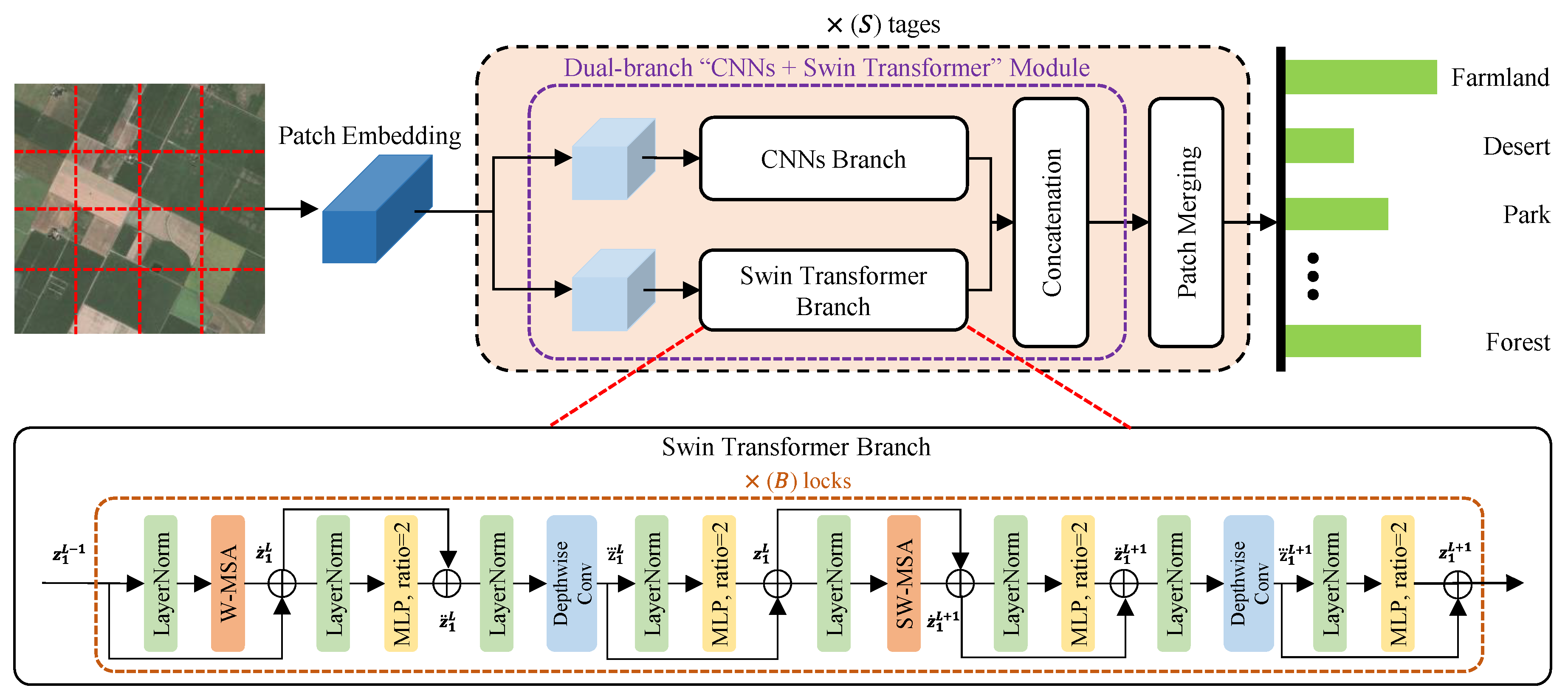
In this section, we will present a comprehensive theoretical explanation of the proposed LDBST architecture and its modules, starting with an overview of the overall network structure, followed by the proposed Dual-branch “CNNs + Swin Transformer” Module.
2.1. Overall Architecture of LDBST
The LDBST model is proposed as a novel lightweight scene classifier, for effectively obtaining semantic context information in HRRS images, and the framework of LDBST is provided in Figure 1. In our LDBST structure, the hierarchical ViT method (Swin-Tiny [27]) is used as the baseline for the LDBST method to explore long-range dependencies in HRRS images. Then, Conv-MLP [33] is integrated into each stage of the LDBST, which enhances the model’s ability to mine long-range dependencies in HRRS images, by strengthening the ViT neighboring window connections. Finally, and most importantly, a dual-branch structure called “CNNs + Swin Transformers” is designed, to split each stage feature in the original Swin-Tiny into two branches, which not only integrates the advantages of a CNN branch for local information and a ViT branch for global information, but also achieves a lightweight model by avoiding the computation of a portion of the fully connected layers and the multi-headed attention mechanism in ViT.
In the LDBST method, a hierarchical vision transformer is constructed using four cascaded stages. The four stages consist of 2, 2, 6, and 2 stacks of swin transformer blocks, respectively. Furthermore, a patch merging method based on linear layers is used to downsample feature maps between each stage, except the last stage.
Given an HRRS image , where H represents the image height, W denotes image width, and C indicates the number of image channels. LDBST first masks a window on the input x of the convolution layer to downsample the input HRRS image to the first stage, and it obtains a set of patches . Then, each patch in P is tokenized using linear embedding. In addition, relative position embeddings are added to these tokens, to represent the positional information. Finally, the embedding vector sequence is fed into the four cascaded stages of the LDBST, and the output dimensions downsampled at each stage are , , , and . Specially, we set n to 4 and C to 96.
2.2. Dual-Branch “CNNs + Swin Transformer” Module
For simplicity, assume that the input for a certain stage of the hierarchical LDBST method is , the dual-branch structure of LDBST splits it into a part and part by a convolutional layer, and the number of channels of the two features is set to be half of . The calculating process can be expressed as follows:
For , the window partitioning approach is adopted to compute the output of layer in the transformer encoder. First, to enhance the capability of the ViT branch in capturing long-range dependency information, additional multilayer perceptrons (MLP) are incorporated into the transformer encoder. Simultaneously, due to the potential drawbacks of increased MLP layers in the ViT branch, which has a limitation on the spatial interaction information, we introduce a depthwise convolution between two MLP blocks, to strengthen the connectivity among neighboring windows, drawing inspiration from Conv-MLP. The calculating process can be defined as
where represents the window-based multi-head self-attention, is the LayerNorm, denotes the multilayer perceptron, indicates depthwise convolution, and T denotes the transpose matrix. is added between two MLPs, which is a convolution layer with the same channel as the two channels of the MLPs, thereby increasing the neighbor window connections.
Then, the shifted window partitioning approach is adopted to compute the output of the layer in the transformer encoder, and the corresponding output of the swin transformer branch is formed by
where denotes the shifted window-based multi-head self-attention. All MLP extension layers in the ViT branches are set to 2, to reduce the number of parameters. Although Formulas (2) and (3) contain many complex computational processes in the ViT branch, the initial input of Formulas (2) and (3) is only half the size of the original input feature of each stage of the LDBST. This means that the proposed dual-branch structure not only enables the model to obtain good feature representation, but also achieves a lightweight model by avoiding certain complex calculations.
Next, for the output of Formula (1), the CNN branch first takes a 3 × 3 convolution layer to extract features, then max pooling is adopted to retain strong features and accelerate the model convergence, finally obtaining the result . Thus, can be calculated using
Finally, the output of the dual-branch “CNNs + Swin Transformer” module is obtained by stacking and in the channel dimension, and this can be formulated as
In summary, the dual-branch module first divides the input feature into two parts and from the channel dimension, then the part is input to the ViT branch of the integrated Conv_MLP, to enhance the connections among neighboring windows and improve the model’s ability to understand global information. To lighten the model and strengthen the ability to understand global information, a convolution layer and a max pooling layer are applied to the part. Since the part only applies a simple convolutional layer and a max pooling layer, this avoids complex multi-head self-attention and MLP computation. Therefore, the computation and parameter number of the LDBST method are significantly reduced when comparing to the baseline Swin-Tiny method.
3. Experiments
3.1. Dataset Description
(1) Aerial Image DataSet (AID DataSet) [34]: The AID dataset contains 30 semantic categories and a total of 10,000 images, and was extracted from Google Earth by Wuhan University. The images are fixed at 600 × 600 pixels, with resolutions ranging from 0.5 to 8 m. The number of images per category varies from 220 to 420.
(2) UC-Merced Land Use DataSet [35]: The UC-Merced Land Use dataset was developed by the University of California, Merced, and contains 21 different land use categories. The dataset contains 2100 color remote sensing images with 256 × 256 pixels, and each category contains 100 images with a resolution of 0.3 m.
(3) NWPU-RESISC45 DataSet [36]: The NWPU-RESISC45 dataset is a scene classification dataset that exhibits rich image diversity and variations. It comprises 31,500 images that are classified into 45 semantic categories. Each class includes 700 images of fixed size (256 × 256 pixels), with a spatial resolution ranging from about 0.2 to 30 m.
(4) RSD46-WHU Dataset [37]: The RSD46-WHU dataset is a public dataset developed by researchers from the School of Remote Sensing Information Engineering, Wuhan University, China, for remote sensing scene classification. The main characteristics of this dataset are being multi-source, high-resolution, large-scale, and highly diverse. The RSD46-WHU dataset contains a total of 117,000 images with a resolution of 0.5 to 2 m, and these images are divided into 46 categories, each with a resolution of 256 × 256 pixels. In the RSD46-WHU Dataset, the number of images per category varies from 500 to 3000.
(5) MLRSN Dataset [38]: The MLRSN dataset consists of 109,161 high-resolution images collected globally by China University of Geosciences. It is divided into 46 categories, with the number sample images ranging from 1500 to 3000 for each category. In addition, the MLRSN dataset provides a wide range of resolutions, from 0.1 m to 10 m. Each image is consistently sized at 256 × 256 pixels, enabling coverage of scenes at different resolutions.
Table 1 shows the specifics of the datasets. The AID, UC-Merced, and NWPU-RESISC45 datasets mentioned above are currently the most widely used datasets for validating model performance. Table 1 indicates that both the MLRSN and RSD46-WHU datasets have a large array of scene categories, with 46 categories each, and a total of 109,161 and 117,000 images, respectively. Meanwhile, the RSD46-WHU dataset and MLRSN dataset are approximately 11-times larger than the AID dataset, approximately 52-times larger than the UC-Merced dataset, and approximately 3.5-times larger than the NWPU-RESISC45 dataset. Therefore, we decided to use the MLRSN and RSD46-WHU datasets as source domains and the AID, UC-Merced, and NWPU-RESISC45 datasets as target domains to explore the transfer learning performance of the LDBST pretrained on these two large-scale remote sensing datasets.
3.2. Experimental Setup
In this paper, the LDBST method was implemented using the Pytorch deep learning framework, and trained on the Ubuntu 20.04 operating system. In addition, all experiments were carried out on a computer equipped with an AMD Ryzen 7 3700X CPU, 16GB RAM, and an NVIDIA GeForce RTX 3060 12GB GPU. We adopted the LDBST method with settings from Swin-Tiny [27]. Specially, the AdamW optimizer was adopted as a cosine decay learning rate scheduler, with an initial learning rate of 0.0005 and a weight decay of 0.05. The data augmentation in [27] was adopted in the LDBST to improve the accuracy. To make full use of the GPU memory, the batch size of the training stage was configured to 100 and the size of the input image was adjusted to 224 × 224 pixels. To gain reliable results, all experiments were repeated five times.
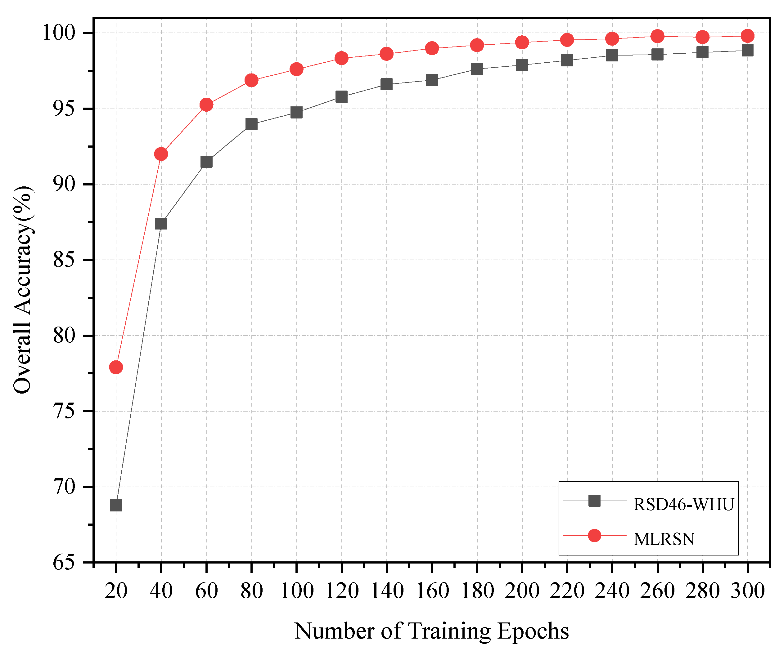
Considering models pretrained on natural image archives, such as ImageNet, have less prior knowledge of aerial scenes [39], we first trained the LDBST model from scratch for 300 epochs using all images in the MLRSN [38] and RSD46-WHU [37] datasets. Based on the data presented in Figure 2, it can be observed that the validation accuracy of the LDBST method was nearly perfect for both datasets. This can be attributed to our utilization of all images as a training set, which also demonstrated that LDBST has an excellent learning ability. Then, two pretrained weights with remote sensing prior information of LDBST were then fine-tuned on the three most commonly used scene classification datasets, i.e., AID [34], UC-Merced [35], and NWPU-RESISC45 [36], for 300 epochs. To ensure a fair comparison of our proposed LDBST method with the existing methods, we adopted the same training set proportions as those used in prior research when dividing the AID, UC-Merced, and NWPU-RESISC45 datasets. Specifically, the AID dataset was partitioned with a 20% and 50% training ratio, the UC-Merced dataset was split with a 50% and an 80% training ratio, and the NWPU-RESISC45 dataset was divided with a 10% and a 20% training ratio.
As shown in Table 2, to comprehensively evaluate the performance of the proposed LDBST method, the transfer learning accuracy of the LDBST method on the AID, UC-Merced, and NWPU-RESISC45 datasets is given. Moreover, the accuracies of two classic networks (e.g., VGG16 and ResNet50) trained with the above-mentioned LDBST hyperparameters is also provided, to verify the effectiveness of the training method. Due to the size of the above HRRS datasets being different, we used different training ratios for each dataset, as seen in Table 2, to understand the adaptability of the LDBST model to different data volumes. Among the three methods in Table 2, although the VGG16 and ResNet50 had been pretrained on two large-scale remote sensing datasets, since these two methods only rely on CNNs to extract local information, their transfer learning performance on the three most commonly used remote sensing datasets was limited when compared with the LDBST under the same training hyperparameter conditions. This was because the LDBST combines a CNN branch to mine local information and a ViT branch to mine long-range dependency information, which improves its performance. According to Table 2, the LDBST method achieved the best classification performance on the NWPU-RESISC45 dataset and UC-Merced dataset when the LDBST method was pretrained using the MLRSN dataset. On the one hand, the LDBST method pretrained using the MLRSN dataset outperformed the LDBST method pretrained using the RSD46-WHU dataset by 0.09% on the UC-Merced dataset (50% training ratio). On the other hand, the LDBST method pretrained using the MLRSN dataset outperformed the LDBST method pretrained using the RSD46-WHU dataset by 3.1% and 0.85%, respectively, on the NWPU-RESISC45 dataset (with training ratios of 10% and 20%). However, when performing transfer learning on the AID dataset, the pretrained model of the LDBST on the MLRSN dataset exhibited a lower transfer performance compared to that on the RSD46-WHU dataset. To be specific, when the training ratio was 20% and 50%, the precision pretrained on the MLRSN dataset was 0.86% and 0.22% lower than that for the RSD46-WHU dataset, respectively. Overall, LDBST achieved satisfactory accuracies on the three most commonly used public datasets after being pretrained on the MLRSN and RSD46-WHU datasets and then transferred. This is because the images in RSD46-WHU are similar in features to those in AID, thus the LDBST pretrained on RSD46-WHU achieved the highest accuracy on the AID dataset. However, MLRSN’s spatial resolution distribution is wider than that of RSD46-WHU, implying that LDBST pretrained on MLRSN may be better transferred to the NWPU-RESISC45 and UC-Merced datasets.
3.3. Comparison with Some State-of-the-Art Methods on the AID Dataset
Table 3 shows an accuracy comparison of the proposed LDBST method with other advanced methods on the AID dataset. We chose to pretrain the LDBST model on the RSD46-WHU dataset as the knowledge transfer benchmark, and then transferred it to the AID dataset. According to Table 3, it is evident that the proposed LDBST method achieved the best accuracy with training ratios of 20% and 50%. In the methods based on transfer learning, T-CNN showed the adaptability of knowledge transfer, having the highest accuracy compared with VGG_VD16+SAFF and EfficientNet-B3-aux methods. In contrast, the proposed LDBST method outperformed the T-CNN by leveraging knowledge from large-scale remote sensing scene classification datasets, which are more reliable than the general image prior knowledge used by T-CNN. According to Table 3, the methods that integrated CNNs with other advanced technologies also achieved good performance in the field of scene classification, such as ACGLNet, CSDS, MSA-Network, EFPN-DSE-TDFF, ACR-MLFF, and other methods. Nevertheless, when compared to the ViT-based methods (e.g., Swin-Tiny and V16_21K), their performance lagged behind. This is because the ViT-based methods use a self-attention mechanism to capture long-range dependencies between different positions in the input sequence. This allows these models to process global information in the image more effectively compared to the aforementioned methods. For a fair comparison, we also compared the performance of the proposed LDBST method with other ViT-based methods. Although the LDBST method had no significant accuracy improvement (maximum 0.21%) compared with the ViT-based V16_21K method, the phenomenon causing this problem was that the LDBST method obtained a superior lightweight performance by reducing the computational effort of the baseline model Swin-T, and thus had less performance advantages in data fitting when compared to the heavyweight V16_21K method with a much greater computational effort. In addition, the LDBST method had a maximum accuracy improvement of 0.24% and 0.22% compared to the Swin-T baseline method at training ratios of 20% and 50%, respectively.
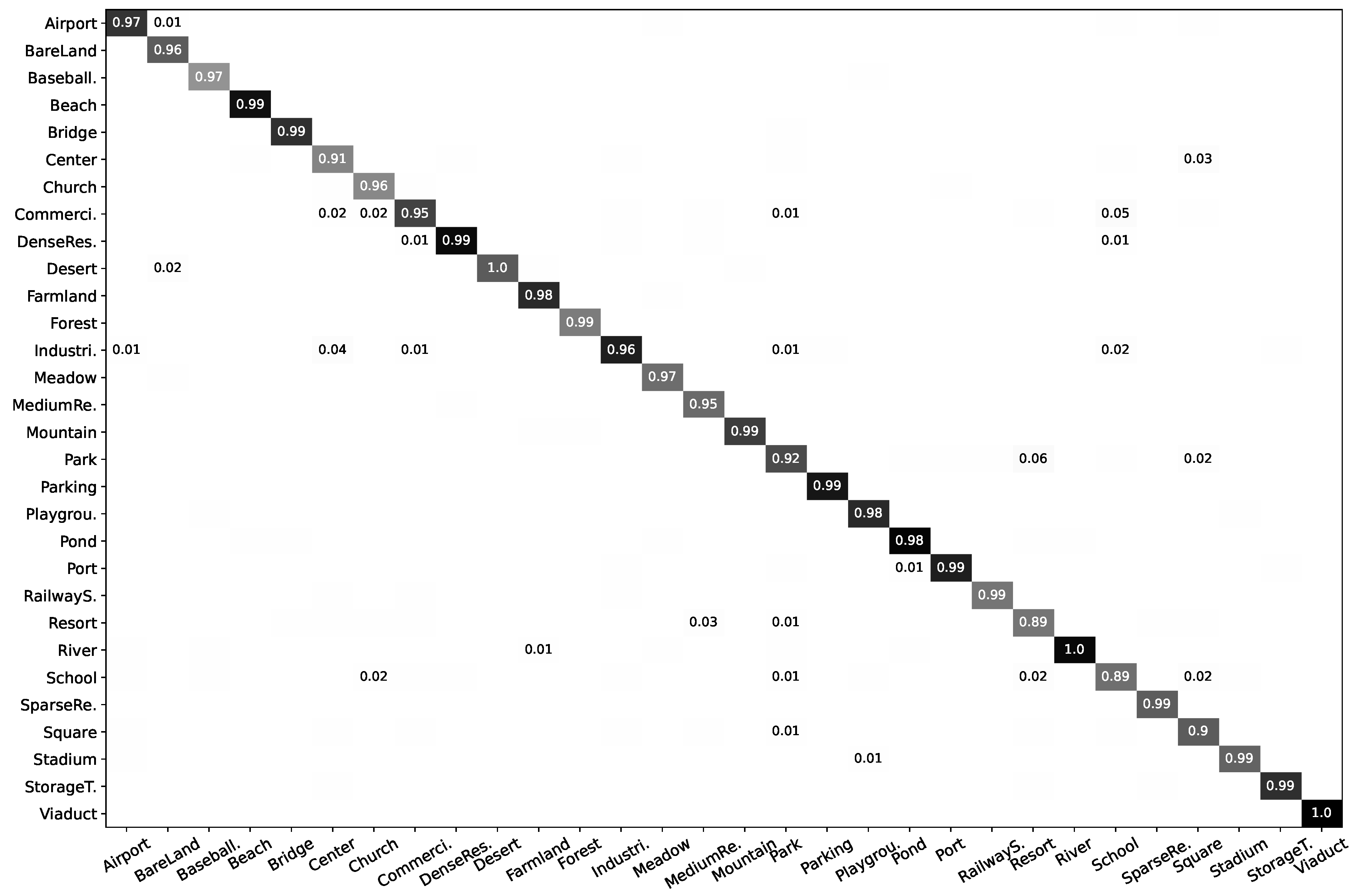
In this paper, we show a confusion matrix of the LDBST method on each dataset. We specify the true labels and predicted labels of the LDBST method as the horizontal and vertical coordinates of the confusion matrix, respectively. For each true label category, the accuracy of the LDBST classification for any category in the dataset is presented as a percentage in the confusion matrix.
The confusion matrix presented in Figure 3 depicts the performance of the LDBST method when trained on the AID dataset with a 50% training ratio. The LDBST method achieved an excellent performance on the AID dataset, where the correct recognition rate exceeded 90% for almost all scenes. Nonetheless, the accuracy for School and Resort was only 89%. The reason for this was that School and Commercial, as well as Resort and Park, share numerous common features, making it challenging for the model to differentiate between them. It was satisfying that LDBST achieved a 100% correct recognition rate for all instances of Desert, River, and Viaduct, which indicates that the LDBST method has a strong scene discrimination capability and robustness.
3.4. Comparison with Some State-of-the-Art Methods on the UC-Merced Dataset
Table 4 shows the experimental results of the LDBST method pretrained on the MLRSN dataset and transferred to the UC-Merced dataset with training rates of 50% and 80%. Specifically, the LDBST method achieved up to 99.14% and 99.76% on the UC-Merced dataset with a training ratio of 50% and 80%, respectively. Among all the methods based on transfer learning, although the T-CNN method achieved the highest accuracy on the UC-Merced dataset, the T-CNN method only achieved a highest accuracy of 99.44% when facing the challenge of the UC-Merced dataset (80% of the training ratio), which was behind the highest accuracy of 99.65% achieved by the CSDS method. However, the proposed LDBST method based on ViT maintained a comprehensive leading advantage compared to both the T-CNN and CSDS methods, achieving the highest accuracies of 99.14% and 99.76% with the two different training ratios, respectively. The proposed lightweight LDBST method had a maximum accuracy improvement of 0.53% compared to the heavyweight V16_21K method at a training ratio of 50%, while the LDBST method had a maximum accuracy improvement of 1.33% and 0.95% compared to the Swin-T baseline method at training ratios of 50% and 80%, respectively. Based on the above analysis, it can be concluded that the LDBST method achieved significant breakthroughs, by combining the advantages of a CNN and enhancing the connection of neighboring windows.
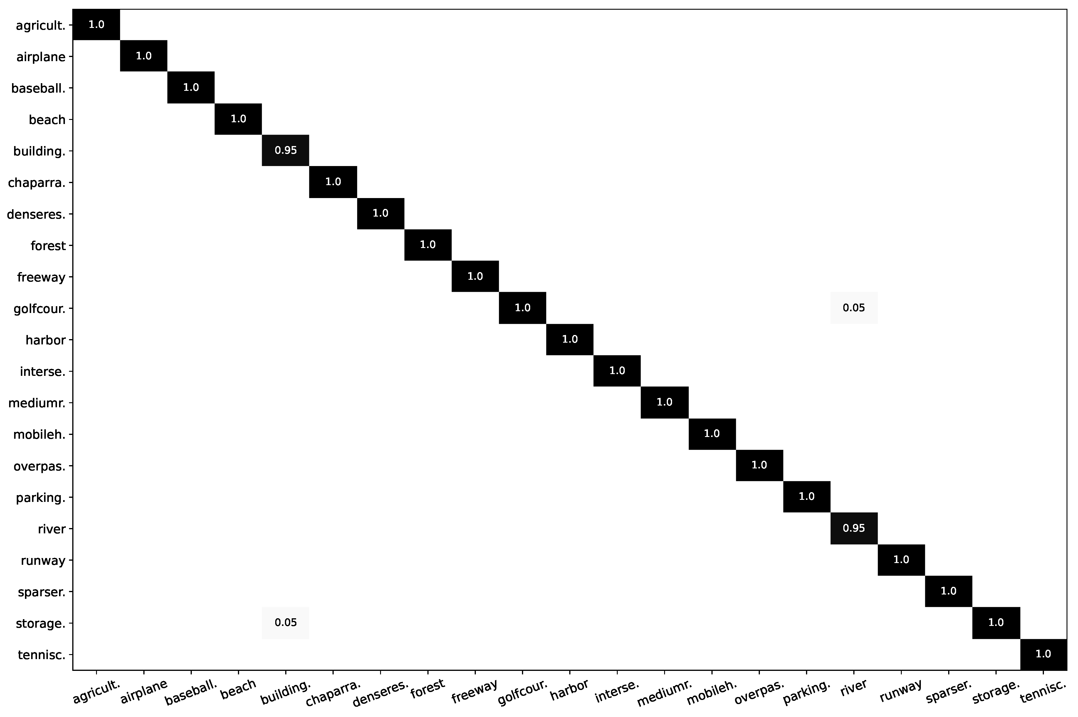
Figure 4 shows the confusion matrix of the LDBST method for the UC-Merced dataset, with a training ratio of 80%. The LDBST method exhibited excellent performance and could accurately and comprehensively identify almost all scenarios in the UC-Merced dataset. It is worth noting that the LDBST method only achieved a maximum classification accuracy of 95% for the scenario building and scenario river. This was because, on the one hand, some storagetanks scenes contain building information; on the other hand, golfcourse scenes and river scenes often contain a lot of green plant information, leading to the network having difficulty distinguishing between the two.
3.5. Comparison with Some State-of-the-Art Methods on the NWPU-RESISC45 Dataset
It can be seen that our proposed LDBST method achieved the best classification performance with both training ratios on the NWPU-RESISC45 dataset, see Table 5. We selected the LDBST model pretrained on the MLRSN dataset as our benchmark for knowledge transfer, and subsequently applied it to the NWPU-RESISC45 dataset.
According to Table 1, the NWPU-RESISC45 dataset was the most challenging of the three target domain datasets, with the number of scenes it contains reaching 46. Moreover, the instances of the NWPU-RESISC45 dataset are nearly 3-times and nearly 14-times larger than that of the AID dataset and UC-Merced dataset, respectively. However, when faced with the challenge of the NWPU-RESISC45 dataset, the performance of the LDBST method still stood out compared to the other state-of-the-art methods. It is worth noting that the MLFCNet50 method benefited from combining general semantic feature information with clustering semantic feature information, achieving the best accuracy among all methods, except for the ViT-based methods. However, the V16_21K method based on ViT had a 0.74% higher accuracy than the MLFCNet50 method under a training ratio of 10%. In comparison with V16_21K, our method improved on it by 1.34%, which demonstrates that our method can effectively improve the scene classification accuracy of remote sensing images.
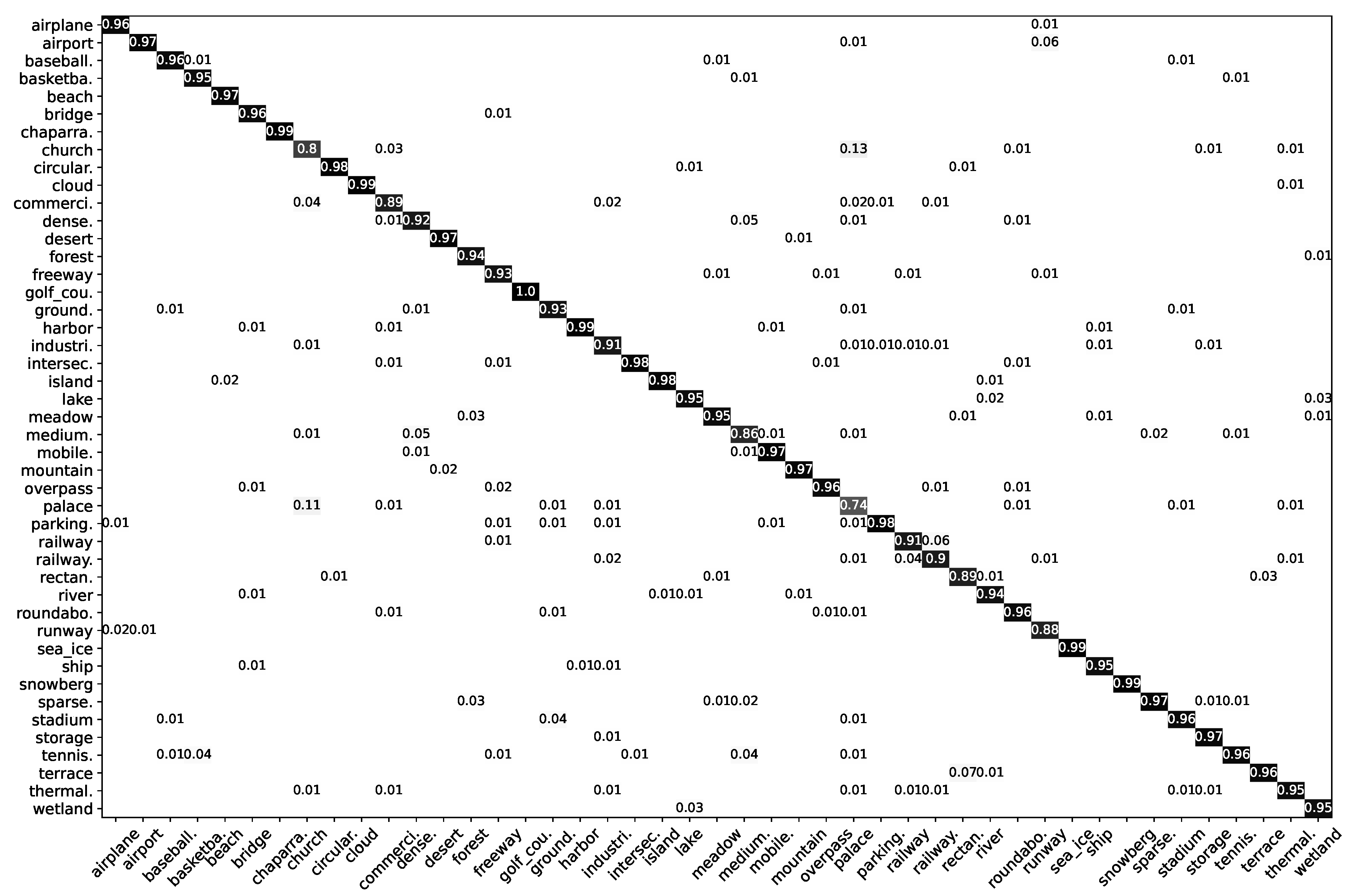
Shown in Figure 5 is a confusion matrix of the LDBST method when the training ratio was 20% on the NWPU-RESISC45 dataset. Due to the strong scene discrimination ability of LDBST, 38 out of 45 scenes in the NWPU-RESISC45 dataset achieved a more than 90% classification accuracy, and 30 out of 45 scenes achieved a more than 95% classification accuracy. However, the accuracies of the scenarios Palace and Church were only 74% and 80%, which greatly affected the overall classification accuracy. The reason for this was that the structure of the Palace is similar to the Church, and there are few internal differences between them.
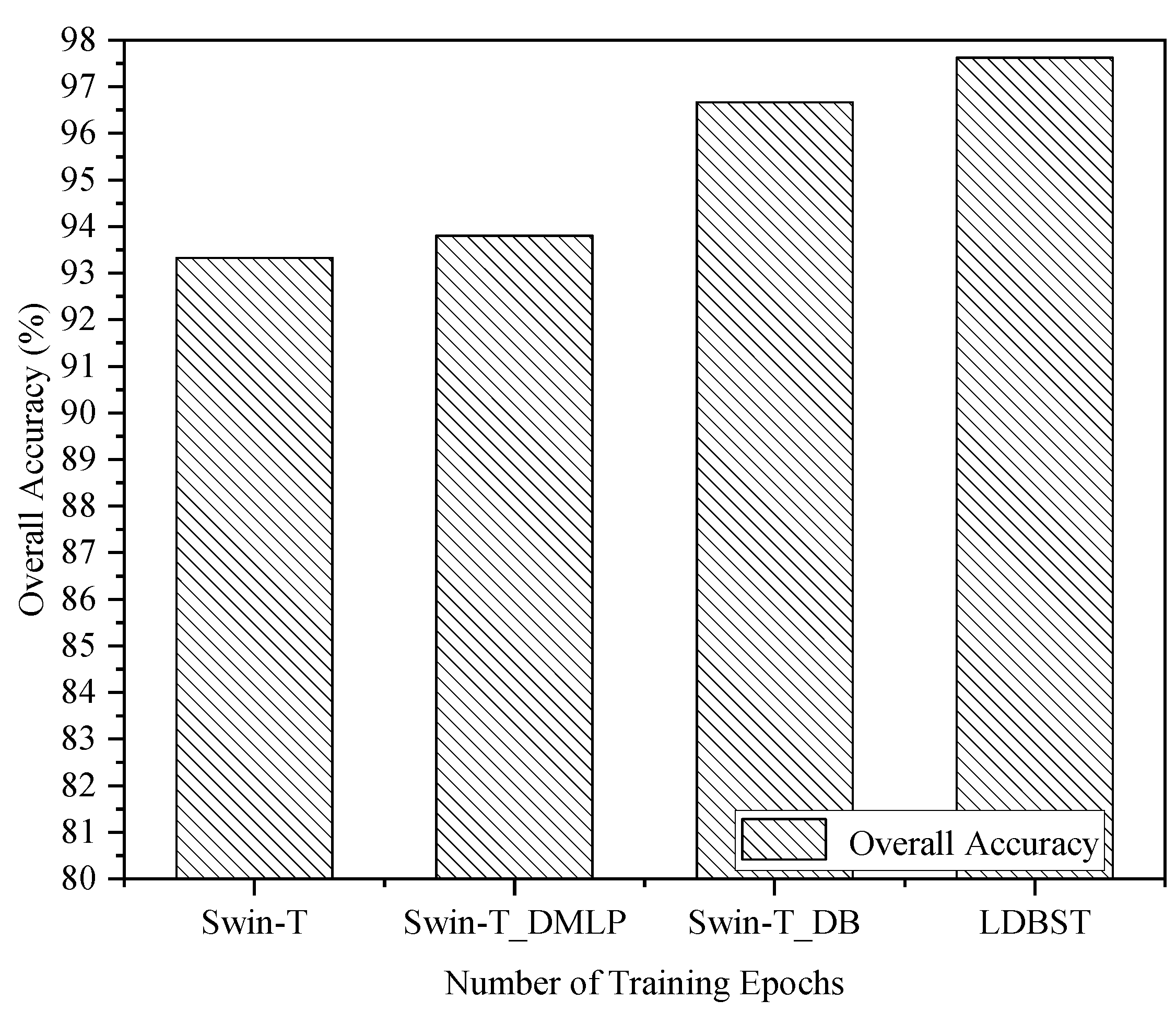
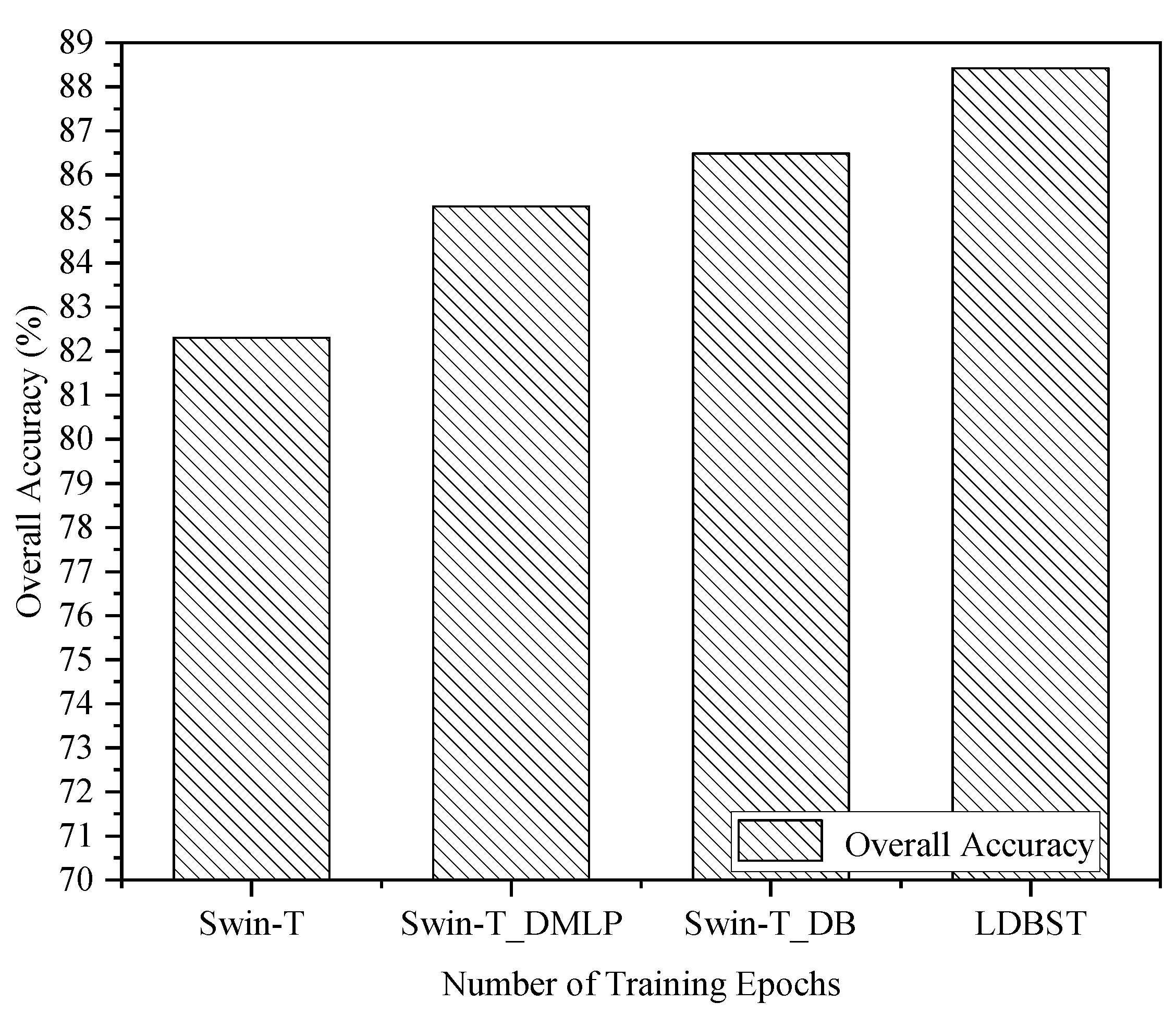
3.6. Ablation Study and Analysis
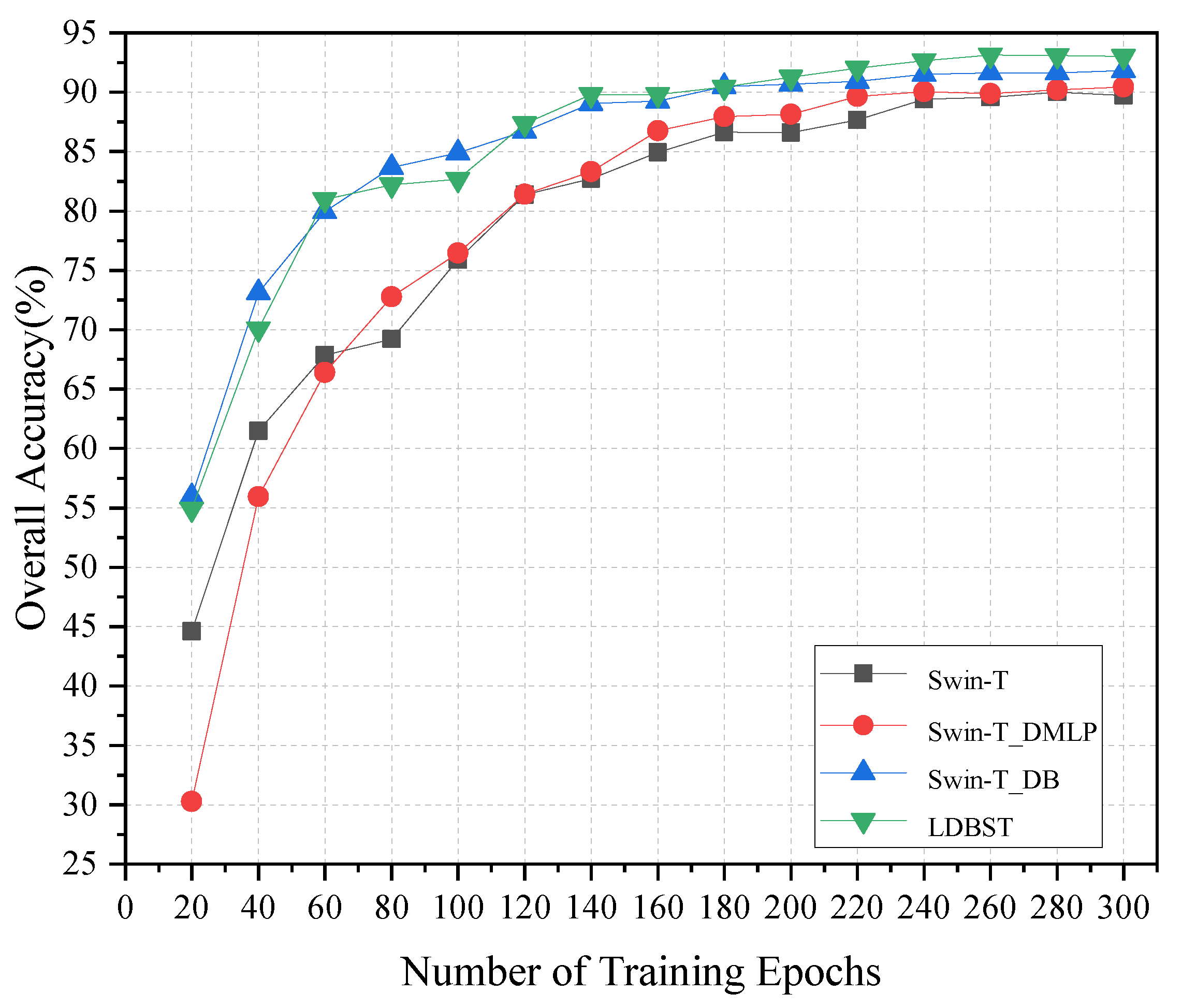
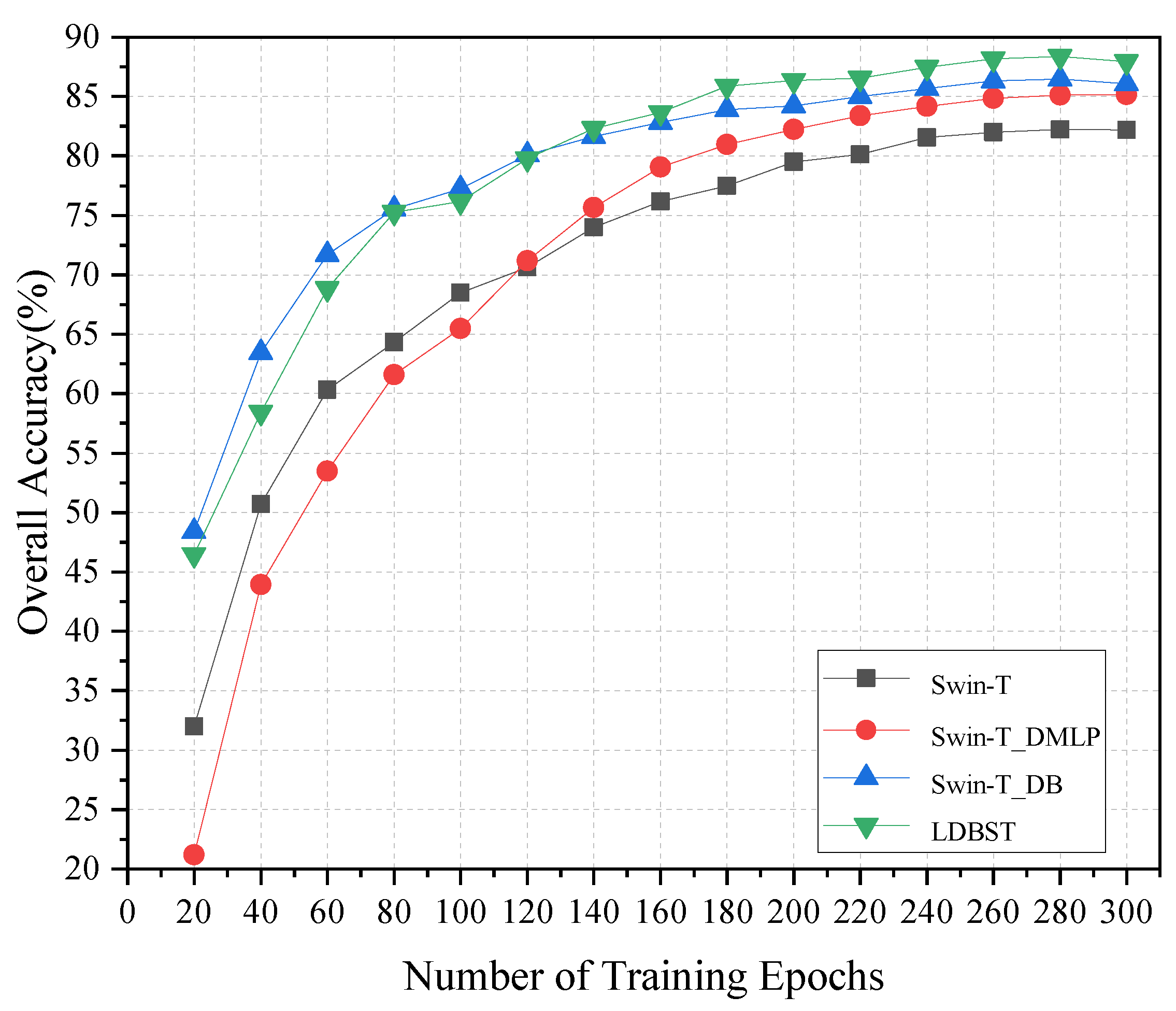
In this paper, some ablation experiments are carried out to further validate the effectiveness of the LDBST method. All experimental models were trained from scratch for a fair comparison, and the AID, UC-Merced, and NWPU-RESISC45 dataset training ratios were set to 50%, 80%, and 20%, respectively. In Figure 6, we present the training accuracy curves for the four models Swin-T, Swin-DMLP, Swin-DB, and LDBST on the AID validation set. The accuracy of each model exhibited a rapid improvement during the first 140 epochs, followed by a slower improvement between epochs 140 and 260, before ultimately converging smoothly between epochs 260 and 300. In addition, in Figure 7 the training curves of the four models on the NWPU-RESISC45 dataset are also presented. The accuracy of each model exhibited a rapid improvement during the first 180 epochs, followed by a slower improvement between epochs 140 and 260, and finally a smooth convergence between epochs 180 and 260.
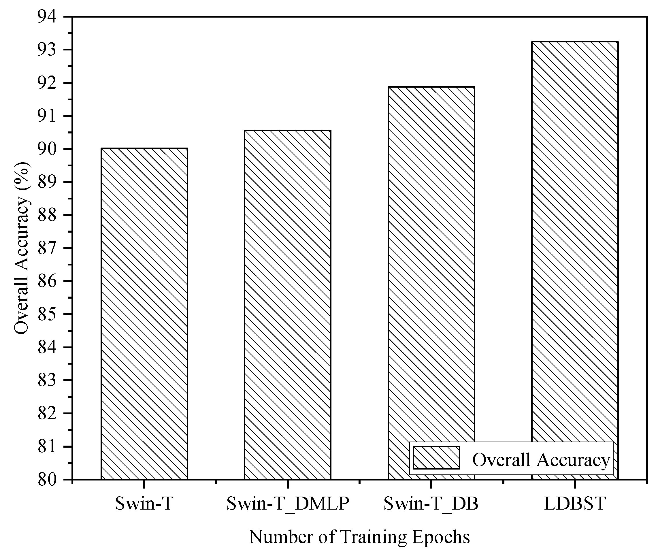
Ablation studies were validated on the AID, UC-Merced, and NWPU-RESISC45 datasets to further reveal the performance contribution of each part of the LDBST, and the results are reported in Figure 8, Figure 9 and Figure 10. Compared with the baseline Swin-T, both Swin-T_DMLP and Swin-T_DB showed a positive performance impact on the three datasets. This is because Swin-T_DMLP improved the ability of scene identification through strengthening the connections of neighboring window using Conv-MLP, and Swin-T_DB improved the ability of scene identification by combining the benefits of ViT and CNNs. Specifically, Swin-T_DMLP improved the accuracies of Swin-T on the AID, UC-Merced, and NWPU-RESISC45 datasets by 0.54%, 0.48%, and 2.97%, respectively. Moreover, compared to Swin-T, Swin-T_DB improved the accuracies for the AID, UC-Merced, and NWPU-RESISC45 datasets by 1.86%, 3.34%, and 4.18%, respectively. When compared with the baseline, the LDBST method, after integrating Conv-MLP and a dual-branch structure, obtained better results, with overall accuracies of 3.22%, 4.29%, and 6.11% higher than the baseline on the AID, UC-Merced, and NWPU-RESISC45 datasets.
3.7. Model Weight Analysis
In order to demonstrate the advantages of LDBST in terms of its light weight, more evidence is given in Table 6. We analyzed the proposed methods using multiple metrics (Parameters, GFLOPs, and Size) at the same input image resolution (224 × 224). According to Table 6, compared with the other state-of-the-art methods (VGG16, Inception V3, ResNet34, and Swin-Tiny), the proposed LDBST method had obvious weight advantages in multiple metrics with the same input size. Especially for the Parameters and Size metrics, LDBST was lower by 66.8% and 66.4% compared with the baseline method Swin-Tiny. This is because the LDBST method adopts a dual-branch structure to split the features in the channel dimension, and only half of the features are used to compute the complex multi-head self-attention and MLP, and the other half of the features are used for a simple convolution layer and a max pooling layer computation.
Table 7 provides a comparison of the inference speed (frames per second, FPS) of the baseline and proposed methods. The improved Swin-T_DB method with dual-branch structure had an inference speed 45% faster than Swin-T. Due to the integration of the Conv-MLP structure in the Swin-T_DMLP method, its inference speed was 19% slower than that of the Swin-T method, but the LDBST method combined with the Conv-MLP and dual-branch structure had an inference speed that was 14.5% faster than that of the Swin-T.
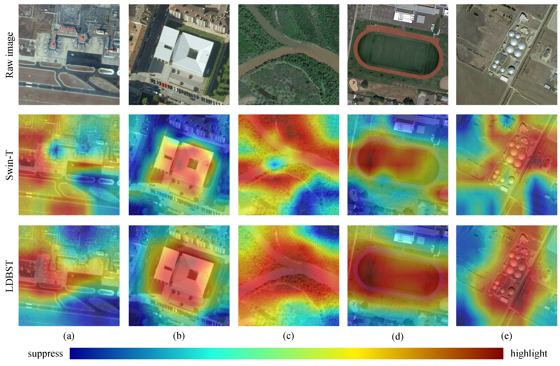
3.8. Visualization Experiment
While deep learning methods have demonstrated superior performance compared to machine learning methods in remote sensing scene classification, one limitation of deep learning is its “feature black box” characteristic. This means that the intermediate processes of the network cannot be intuitively explained. In order to intuitively demonstrate the advantages of LDBST from the perspective of human vision, we used Grad-ACM [43] to interpret the LDBST method in depth network vision, based on gradient localization. Grad-ACM displays the positioning of key area information in an image by generating a het map.
As shown in Figure 11, we display the het maps of the LDBST method and the Swin-T (baseline) method on five sets of images, with data samples from the categories Airport, Center, River, Playground, and Storage Tanks of the AID dataset. In Figure 11, the first line is the original images, the second line is the het maps of the Swin-T method, and the third line is the het maps of the LDBST method. A redder location in the het map indicates that the network is more focused, while a bluer location indicates that the network is less focused. It is obvious that in the column (a) experiments, the Swin-T method did not mainly focus on the aircraft in the airport images, and its focus area was relatively scattered. However, LDBST was able to focus on both the runway and aircraft parts of the airport images. In the column (b) experiments, while both methods focused on the central area of the image, it is evident that the LDBST method concentrated on more reasonable areas and also included the auxiliary information area of the road surface around the building. The column (c) experiment depicted a Y-shaped river, and the LDBST method gave greater emphasis to the middle part of the scene compared to the Swin-T method. During the experiments conducted in columns (d) and (e), the Swin-T method displayed inadequate attention to the focus areas of both image columns. Furthermore, the LDBST method exhibited a more targeted focus than the Swin-T method, and it provided comprehensive coverage of the focus areas for both image columns. Capturing long-range dependencies between features in an image is necessary for global understanding of a visual scene [44]. In the experiments in columns (b) and (d), the LDBST method combined the strong sensitivity advantage of CNNs for local features and the advantage of ViT in capturing long-range dependencies, resulting in the model’s accurate attention to the key regions in the context scenarios of center and playground having a larger span advantage in spatial scale compared to the Swin-Tiny method.
4. Conclusions
In this paper, a novel lightweight dual-branch swin transformer network (LDBST) integrating a CNN and ViT is proposed for remote scene classification. The dual-branch LDBST, not only improves the scene discrimination ability, but also reduces the computation complexity. First, the LDBST improved the performance by integrating Conv-MLP to enhance the connections between the neighboring windows of the ViT branch. Then, to obtain better feature representation, LDBST was pretrained on the remote scene classification images of the MLRSN and RSD46-WHU datasets. The two pretrained weights were transferred on the target remote sensing scene classification datasets. Compared with existing ViT-based methods, LDBST had a huge weight advantage. Finally, the experimental results revealed that the proposed LDBST method outperformed some state-of-the-art pretrained Imagenet methods on the UC-Merced, AID, and NWPU-RESISC45 datasets.
In the future, given the success of the dual-branch structure proposed in this paper for creating high-performance and lightweight scene classification methods, we aim to examine the potential of this dual-branch structure in object detection of HRRS images and to develop sophisticated, real-time models for advanced industrial applications.
Author Contributions
Conceptualization, F.Z.; methodology, F.Z.; software, F.Z.; validation, F.Z.; formal analysis, S.L.; investigation, S.L.; resources, W.Z. and H.H.; data curation, S.L.; writing—original draft preparation, F.Z.; writing—review and editing, W.Z. and H.H.; visualization, S.L.; supervision, H.H.; project administration, H.H.; funding acquisition, W.Z. and H.H. All authors have read and agreed to the published version of the manuscript.
Funding
This research was supported in part by the Natural Science Foundation of Chongqing under Grant cstc2019jcyj-msxmX0080, the National Natural Science Foundation of China under Grant 42071302, the Science and Technology Research Program of Chongqing Municipal Education Commission under Grant KJZD-K202001501 and KJCX2020051, and Cooperation project between Chongqing Municipal undergraduate universities and institutes affiliated to the Chinese Academy of Sciences under Grant HZ2021015.
Institutional Review Board Statement
Not applicable.
Informed Consent Statement
Not applicable.
Data Availability Statement
The data generated and analyzed during this study are available from the corresponding author by request.
Conflicts of Interest
The authors declare no conflict of interest.
References
- Zhang, F.; Du, B.; Zhang, L. Saliency-guided unsupervised feature learning for scene classification. IEEE Trans. Geosci. Remote Sens. 2014, 53, 2175–2184. [Google Scholar] [CrossRef]
- Fan, Z.; Yu, J.-G.; Liang, Z.; Ou, J.; Gao, C.; Xia, G.-S.; Li, Y. FGN: Fully guided network for few-shot instance segmentation. In Proceedings of the IEEE/CVF Conference on Computer Vision and Pattern Recognition (CVPR), Virtual, 14–19 June 2020; pp. 9172–9181. [Google Scholar]
- Ye, F.; Xiao, H.; Zhao, X.; Dong, M.; Luo, W.; Min, W. Remote sensing image retrieval using convolutional neural network features and weighted distance. IEEE Geosci. Remote Sens. Lett. 2018, 15, 1535–1539. [Google Scholar] [CrossRef]
- Cheng, G.; Yao, Y.; Li, S.; Li, K.; Xie, X.; Wang, J.; Yao, X.; Han, J. Dual-Aligned Oriented Detector. IEEE Trans. Geosci. Remote Sens. 2022, 60, 1–11. [Google Scholar] [CrossRef]
- Wu, C.; Du, B.; Zhang, L. Fully convolutional change detection framework with generative adversarial network for unsupervised, weakly supervised and regional supervised change detection. arXiv 2022, arXiv:2201.06030. [Google Scholar] [CrossRef]
- Lv, P.; Wu, W.; Zhong, Y.; Du, F.; Zhang, L. Scvit: A spatial-channel feature preserving vision transformer for remote sensing image scene classification. IEEE Trans. Geosci. Remote Sens. 2022, 60, 1–12. [Google Scholar] [CrossRef]
- Bi, Q.; Qin, K.; Li, Z.; Zhang, H.; Xu, K.; Xia, G.-S. A multiple-instance densely-connected ConvNet for aerial scene classification. IEEETrans. Image Process. 2020, 29, 4911–4926. [Google Scholar] [CrossRef]
- Zhong, Y.; Zhu, Q.; Zhang, L. Scene classification based on the multifeature fusion probabilistic topic model for high spatial resolution remote sensing imagery. IEEE Trans. Geosci. Remote Sens. 2015, 53, 6207–6222. [Google Scholar] [CrossRef]
- Huang, L.; Chen, C.; Li, W.; Du, Q. Remote sensing image scene classification using multi-scale completed local binary patterns and fisher vectors. Remote Sens. 2016, 8, 483. [Google Scholar] [CrossRef]
- Sun, H.; Li, S.; Zheng, X.; Lu, X. Remote sensing scene classification by gated bidirectional network. IEEE Trans. Geosci. Remote Sens. 2019, 58, 82–96. [Google Scholar] [CrossRef]
- Bazi, Y.; Al Rahhal, M.M.; Alhichri, H.; Alajlan, N. Simple yet effective fine-tuning of deep CNNs using an auxiliary classification loss for remote sensing scene classification. Remote Sens. 2019, 11, 2908. [Google Scholar] [CrossRef]
- Wang, W.; Chen, Y.; Ghamisi, P. Transferring cnn with adaptive learning for remote sensing scene classification. IEEE Trans. Geosci. Remote Sens. 2022, 60, 1–18. [Google Scholar] [CrossRef]
- Deng, P.; Xu, K.; Huang, H. When CNNs meet vision transformer: A joint framework for remote sensing scene classification. IEEE Geosci.Remote Sens. Lett. 2021, 19, 1–5. [Google Scholar] [CrossRef]
- Li, E.; Samat, A.; Du, P.; Liu, W.; Hu, J. Improved bilinear CNN model for remote sensing scene classification. IEEE Geosci. Remote Sens. Lett. 2020, 19, 1–5. [Google Scholar] [CrossRef]
- Wang, X.; Wang, S.; Ning, C.; Zhou, H. Enhanced Feature Pyramid Network with Deep Semantic Embedding for Remote Sensing Scene Classification. IEEE Trans. Geosci. Remote Sens. 2021, 59, 7918–7932. [Google Scholar] [CrossRef]
- Xu, K.; Huang, H.; Deng, P.; Li, Y. Deep feature aggregation framework driven by graph convolutional network for scene classification in remote sensing. IEEE Trans. Neural Netw. Learn. Syst. 2021, 33, 5751–5765. [Google Scholar] [CrossRef] [PubMed]
- Wang, X.; Duan, L.; Shi, A.; Zhou, H. Multilevel feature fusion networks with adaptive channel dimensionality reduction for remote sensing scene classification. IEEE Geosci. Remote Sens. Lett. 2022, 19, 1–5. [Google Scholar] [CrossRef]
- Shen, J.; Yu, T.; Yang, H.; Wang, R.; Wang, Q. An attention cascade global–local network for remote sensing scene classification. Remote Sens. 2022, 14, 2042. [Google Scholar] [CrossRef]
- Wang, D.; Zhang, C.; Han, M. Mlfc-net: A multi-level feature combination attention model for remote sensing scene classification. Comput. Geosci. 2022, 160, 105042. [Google Scholar] [CrossRef]
- Cao, R.; Fang, L.; Lu, T.; He, N. Self-attention-based deep feature fusion for remote sensing scene classification. IEEE Geosci. Remote Sens. Lett. 2020, 18, 43–47. [Google Scholar] [CrossRef]
- Zhang, G.; Xu, W.; Zhao, W.; Huang, C.; Yk, E.N.; Chen, Y.; Su, J. A Multiscale Attention Network for Remote Sensing Scene Images Classification. IEEE J. Sel. Top. Appl. Earth Observ. Remote Sens. 2021, 14, 9530–9545. [Google Scholar] [CrossRef]
- Wang, H.; Gao, K.; Min, L.; Mao, Y.; Zhang, X.; Wang, J.; Hu, Z.; Liu, Y. Triplet-metric-guided multi-scale attention for remote sensing image scene classification with a convolutional neural network. Remote Sens. 2022, 14, 2794. [Google Scholar] [CrossRef]
- Wang, X.; Duan, L.; Ning, C.; Zhou, H. Relation-Attention Networks for Remote Sensing Scene Classification. IEEE J. Sel. Top. Appl. Earth Observ. Remote Sens. 2021, 15, 422–439. [Google Scholar] [CrossRef]
- Wang, X.; Yuan, L.; Xu, H.; Wen, X. CSDS: End-to-End Aerial Scenes Classification with Depthwise Separable Convolution and an Attention Mechanism. IEEE J. Sel. Top. Appl. Earth Observ. Remote Sens. 2021, 14, 10484–10499. [Google Scholar] [CrossRef]
- Guo, J.; Han, K.; Wu, H.; Tang, Y.; Chen, X.; Wang, Y.; Xu, C. Cmt: Convolutional neural networks meet vision transformers. In Proceedings of the IEEE/CVF Conference on Computer Vision and Pattern Recognition (CVPR), New Orleans, LA, USA, 19–24 June 2022; pp. 12175–12185. [Google Scholar]
- Dosovitskiy, A.; Beyer, L.; Kolesnikov, A.; Weissenborn, D.; Zhai, X.; Unterthiner, T.; Dehghani, M.; Minderer, M.; Heigold, G.; Gelly, S.; et al. An image is worth 16x16 words: Transformers for image recognition at scale. In Proceedings of the International Conference on Learning Representations (ICLR), Virtual, 3–7 May 2021. [Google Scholar]
- Liu, Z.; Lin, Y.; Cao, Y.; Hu, H.; Wei, Y.; Zhang, Z.; Lin, S.; Guo, B. Swin transformer: Hierarchical vision transformer using shifted windows. In Proceedings of the International Conference on Computer Vision (ICCV), Montreal, BC, Canada, 11–17 October 2021; pp. 10012–10022. [Google Scholar]
- Bazi, Y.; Bashmal, L.; Rahhal, M.M.A.; Dayil, R.A.; Ajlan, N.A. Vision transformers for remote sensing image classification. Remote Sens. 2021, 13, 516. [Google Scholar] [CrossRef]
- Zhang, J.; Zhao, H.; Li, J. TRS: Transformers for Remote Sensing Scene Classification. Remote Sens. 2021, 13, 4143. [Google Scholar] [CrossRef]
- Sha, Z.; Li, J. Mitformer: A multiinstance vision transformer for remote sensing scene classification. IEEE Geosci. Remote Sens. Lett. 2022, 19, 1–5. [Google Scholar] [CrossRef]
- Bi, M.; Wang, M.; Li, Z.; Hong, D. Vision transformer with contrastive learning for remote sensing image scene classification. IEEE J. Sel. Top. Appl. Earth Observ. Remote Sens. 2023, 16, 738–749. [Google Scholar] [CrossRef]
- Zhao, M.; Meng, Q.; Zhang, L.; Hu, X.; Bruzzone, L. Local and long-range collaborative learning for remote sensing scene classification. IEEE Trans. Geosci. Remote Sens. 2023, 61, 1–15. [Google Scholar] [CrossRef]
- Li, J.; Hassani, A.; Walton, S.; Shi, H. ConvMLP: Hierarchical convolutional mlps for vision. arXiv 2021, arXiv:2109.04454. [Google Scholar]
- Xia, G.-S.; Hu, J.; Hu, F.; Shi, B.; Bai, X.; Zhong, Y.; Zhang, L.; Lu, X. AID: A benchmark data set for performance evaluation of aerial scene classification. IEEE Trans. Geosci. Remote Sens. 2017, 55, 3965–3981. [Google Scholar] [CrossRef]
- Yang, Y.; Newsam, S. Bag-of-visual-words and spatial extensions for land-use classification. In Proceedings of the 18th SIGSPATIAL International Conference on Advances in Geographic Information Systems, San Jose, CA, USA, 2–5 November 2010; pp. 270–279. [Google Scholar]
- Cheng, G.; Han, J.; Lu, X. Remote sensing image scene classification: Benchmark and state of the art. Proc. IEEE 2017, 105, 1865–1883. [Google Scholar] [CrossRef]
- Long, Y.; Gong, Y.; Xiao, Z.; Liu, Q. Accurate object localization in remote sensing images based on convolutional neural networks. IEEE Trans. Geosci. Remote Sens. 2017, 55, 2486–2498. [Google Scholar] [CrossRef]
- Qi, X.; Zhu, P.; Wang, Y.; Zhang, L.; Peng, J.; Wu, M.; Chen, J.; Zhao, X.; Zang, N.; Mathiopoulos, P.T. MLRSNet: A multi-label high spatial resolution remote sensing dataset for semantic scene understanding. ISPRS J. Photogramm. Remote Sens. 2020, 169, 337–350. [Google Scholar] [CrossRef]
- Long, Y.; Xia, G.-S.; Zhang, L.; Cheng, G.; Li, D. Aerial Scene Parsing: From Tile-level Scene Classification to Pixel-wise Semantic Labeling. arXiv 2022, arXiv:2201.01953. [Google Scholar]
- He, K.; Zhang, X.; Ren, S.; Sun, J. Deep residual learning for image recognition. In Proceedings of the IEEE Conference on Computer Vision and Pattern Recognition (CVPR), Las Vegas, NV, USA, 27–30 June 2016; pp. 770–778. [Google Scholar]
- Simonyan, K.; Zisserman, A. Very deep convolutional networks for large-scale image recognition. In Proceedings of the International Conference on Learning Representations (ICLR), San Diego, CA, USA, 7–9 May 2015. [Google Scholar]
- Szegedy, C.; Vanhoucke, V.; Ioffe, S.; Shlens, J.; Wojna, Z. Rethinking the inception architecture for computer vision. In Proceedings of the IEEE Conference on Computer Vision and Pattern Recognition (CVPR), Las Vegas, NV, USA, 27–30 June 2016; pp. 2818–2826. [Google Scholar]
- Selvaraju, R.R.; Cogswell, M.; Das, A.; Vedantam, R.; Parikh, D.; Batra, D. Grad-cam: Visual explanations from deep networks via gradient-based localization. In Proceedings of the International Conference on Computer Vision (ICCV), Venice, Italy, 22–29 October 2017; pp. 618–626. [Google Scholar]
- Cao, Y.; Xu, J.; Lin, S.; Wei, F.; Hu, H. Gcnet: Non-local networks meet squeeze-excitation networks and beyond. In Proceedings of the International Conference on Computer Vision (ICCV), Seoul, Republic of Korea, 27 October–2 November 2019. [Google Scholar]
Figure 1.
Framework of the proposed LDBST method. LDBST consists of S cascading stages, where the “swin transformer branch” is repeated B times before a concatenation is utilized to express the stage S. More specifically, we set S to 4, and B in each stage is set to 2, 2, 6, and 2, respectively.
Figure 1.
Framework of the proposed LDBST method. LDBST consists of S cascading stages, where the “swin transformer branch” is repeated B times before a concatenation is utilized to express the stage S. More specifically, we set S to 4, and B in each stage is set to 2, 2, 6, and 2, respectively.

Figure 2.
The training curves of LDBST for all images in the RSD46-WHU and MLRSN datasets.

Figure 3.
Confusion matrix of AID dataset using the proposed LDBST method at a training rate of 50%. It is worth noting that the values in the confusion matrix have been rounded to show two decimal places, thus smaller values are ignored.
Figure 3.
Confusion matrix of AID dataset using the proposed LDBST method at a training rate of 50%. It is worth noting that the values in the confusion matrix have been rounded to show two decimal places, thus smaller values are ignored.

Figure 4.
Confusion matrix of UC-Merced dataset using the proposed LDBST method at a training rate of 80%.
Figure 4.
Confusion matrix of UC-Merced dataset using the proposed LDBST method at a training rate of 80%.

Figure 5.
Confusion matrix of the NWPU-RESISC45 dataset using the proposed LDBST method at a training rate of 20%.
Figure 5.
Confusion matrix of the NWPU-RESISC45 dataset using the proposed LDBST method at a training rate of 20%.

Figure 6.
Ablation experiment training curve of the AID dataset.

Figure 7.
Ablation experiment training curve for the NWPU-RESISC45 Dataset.

Figure 8.
Ablation study on the AID Dataset.

Figure 9.
Ablation study on the UC-Merced Dataset.

Figure 10.
Ablation study on the NWPU-RESISC45 Dataset.

Figure 11.
Heat map of five scenarios in the AID dataset presented using the Grad-ACM technique. (a) Airport. (b) Center. (c) River. (d) Playground. (e) Storage Tanks.
Figure 11.
Heat map of five scenarios in the AID dataset presented using the Grad-ACM technique. (a) Airport. (b) Center. (c) River. (d) Playground. (e) Storage Tanks.


Table 1.
Details of the datasets.
| Dataset | Categories | Images per Cat. | Instances | Image Size | Resolution (m) |
|---|---|---|---|---|---|
| AID | 30 | 220–420 | 10,000 | 600 × 600 | 0.5–8 |
| UC-Merced | 21 | 100 | 2100 | 256 × 256 | 0.3 |
| NWPU-RESISC45 | 45 | 700 | 31,500 | 256 × 256 | 0.2–30 |
| RSD46-WHU | 46 | 500–3000 | 117,000 | 256 × 256 | 0.5–2 |
| MLRSN | 46 | 1500–3000 | 109,161 | 256 × 256 | 0.1–10 |
Table 2.
Performance comparison of the proposed method on different pretrained datasets.
| Pretrained Dataset | Method | AID (20%) | AID (50%) | UC-Merced (50%) | UC-Merced (80%) | NWPU-RESISC45 (10%) | NWPU-RESISC45 (20%) |
|---|---|---|---|---|---|---|---|
| MLRSN | ResNet50 [40] | 73.95 ± 0.17 | 80.32 ± 0.36 | 86.19 ± 0.29 | 93.57 ± 0.24 | 67.46 ± 0.15 | 73.54 ± 0.17 |
| VGG16 [41] | 77.60 ± 0.11 | 82.30 ± 0.26 | 87.43 ± 0.10 | 94.52 ± 0.23 | 73.42 ± 0.10 | 77.90 ± 0.14 | |
| RSD46-WHU | ResNet50 [40] | 74.35 ± 0.11 | 80.12 ± 0.26 | 87.14 ± 0.28 | 94.76 ± 0.24 | 65.65 ± 0.12 | 72.03 ± 0.12 |
| VGG16 [41] | 74.42 ± 0.22 | 80.17 ± 0.18 | 90.86 ± 0.19 | 96.67 ± 0.28 | 72.11 ± 0.14 | 77.10 ± 0.13 | |
Table 3.
Overall classification accuracy (%) comparison with the AID dataset.
| Method | 20% Training Ratio | 50% Training Ratio |
|---|---|---|
| Fine-tuning VGG16 [10] | 89.49 ± 0.34 | 93.60 ± 0.64 |
| GBNet [10] | 90.16 ± 0.24 | 93.72 ± 0.34 |
| VGG_VD16+SAFF [20] | 90.25 ± 0.29 | 93.83 ± 0.28 |
| DFAGCN [16] | - | 94.88 ± 0.22 |
| RANet [23] | 92.71 ± 0.14 | 95.31 ± 0.37 |
| ACR-MLFF [17] | 92.73 ± 0.12 | 95.06 ± 0.33 |
| GoogLeNet-aux [11] | 93.25 ± 0.33 | 95.54 ± 0.12 |
| MSA-Network [21] | 93.53 ± 0.21 | 96.01 ± 0.43 |
| EFPN-DSE-TDFF [15] | 94.02 ± 0.21 | 94.50 ± 0.30 |
| EfficientNet-B0-aux [11] | 93.69 ± 0.11 | 96.17 ± 0.16 |
| EfficientNet-B3-aux [11] | 94.19 ± 0.15 | 96.56 ± 0.14 |
| CSDS [24] | 94.29 ± 0.35 | 96.70 ± 0.14 |
| ACGLNet [18] | 94.44 ± 0.09 | 96.10 ± 0.10 |
| T-CNN [12] | 94.55 ± 0.27 | 96.72 ± 0.23 |
| Swin-Tiny [27] | 94.80 ± 0.15 | 96.70 ± 0.12 |
| V16_21K[224 × 224] [28] | 94.97 ± 0.01 | - |
Table 4.
Overall classification accuracy (%) comparison with the UC-Merced dataset.
| Method | 50% Training Ratio | 80% Training Ratio |
|---|---|---|
| GBNet [10] | 95.71 ± 0.19 | 96.90 ± 0.23 |
| VGG_VD16+SAFF [20] | - | 97.02 ± 0.78 |
| DFAGCN [16] | - | 98.48 ± 0.42 |
| EFPN-DSE-TDFF [15] | 96.19 ± 0.13 | 99.14 ± 0.22 |
| Fine-tuning VGG16 [10] | 96.57 ± 0.38 | 97.14 ± 0.48 |
| RANet [23] | 97.80 ± 0.19 | 99.27 ± 0.24 |
| MSA-Network [21] | 97.80 ± 0.33 | 98.96 ± 0.21 |
| GoogLeNet-aux [11] | 97.90 ± 0.34 | 99.00 ± 0.46 |
| T-CNN [12] | - | 99.33 ± 0.11 |
| ACR-MLFF [17] | 97.99 ± 0.26 | 99.37 ± 0.15 |
| MLFCNet50 [19] | 98.06 ± 0.41 | 99.37 ± 0.22 |
| ACGLNet [18] | 98.14 ± 0.25 | 99.46 ± 0.12 |
| EfficientNet-B0-aux [11] | 98.01 ± 0.45 | 99.04 ± 0.33 |
| EfficientNet-B3-aux [11] | 98.22 ± 0.49 | 99.09 ± 0.17 |
| CSDS [24] | 98.48 ± 0.21 | 99.52 ± 0.13 |
| Swin-Tiny [27] | 97.52 ± 0.29 | 98.57 ± 0.24 |
| V16_21K[224 × 224] [28] | 98.14 ± 0.47 | - |
Table 5.
Overall classification accuracy (%) comparison with the NWPU-RESISC45 dataset.
| Method | 10% Training Ratio | 20% Training Ratio |
|---|---|---|
| VGG_VD16+SAFF [20] | 84.38 ± 0.19 | 87.86 ± 0.14 |
| DFAGCN [16] | - | 89.29 ± 0.28 |
| GoogLeNet-aux [11] | 89.22 ± 0.25 | 91.63 ± 0.11 |
| ACR-MLFF [17] | 90.01 ± 0.33 | 92.45 ± 0.20 |
| EfficientNet-B0-aux [11] | 89.96 ± 0.27 | 92.89 ± 0.16 |
| EfficientNet-B3-aux [11] | 91.08 ± 0.14 | 93.81 ± 0.07 |
| T-CNN [12] | 90.25 ± 0.14 | 93.05 ± 0.12 |
| MSA-Network [21] | 90.38 ± 0.17 | 93.52 ± 0.21 |
| CSDS [24] | 91.64 ± 0.16 | 93.59 ± 0.21 |
| MLFCNet50 [19] | 91.66 ± 0.30 | 94.32 ± 0.04 |
| Swin-Tiny [27] | 89.54 ± 0.14 | 92.64 ± 0.07 |
| V16_21K[224 × 224] [28] | 92.60 ± 0.10 | - |
Table 6.
Comparison of the parameters, GFLOPs, and size with other models.
| Method | Image Size | Params (M) | GFLOPs | Size (MB) |
|---|---|---|---|---|
| VGG16 [41] | 224 × 224 | 138.4 | 15.5 | 528.0 |
| Inception V3 [42] | 224 × 224 | 23.8 | 2.9 | 104.0 |
| ResNet34 [40] | 224 × 224 | 21.8 | 3.7 | 83.3 |
| Swin-Tiny [27] | 224 × 224 | 28.0 | 4.5 | 114.3 |
Table 7.
The inference speed of the proposed methods.
| Swin-T | Swin-T_DMLP | Swin-T_DB | LDBST | |
|---|---|---|---|---|
| FPS | 427 | 346 | 619 | 489 |
Disclaimer/Publisher’s Note: The statements, opinions and data contained in all publications are solely those of the individual author(s) and contributor(s) and not of MDPI and/or the editor(s). MDPI and/or the editor(s) disclaim responsibility for any injury to people or property resulting from any ideas, methods, instructions or products referred to in the content. |
© 2023 by the authors. Licensee MDPI, Basel, Switzerland. This article is an open access article distributed under the terms and conditions of the Creative Commons Attribution (CC BY) license (https://creativecommons.org/licenses/by/4.0/).
Share and Cite
MDPI and ACS Style
Zheng, F.; Lin, S.; Zhou, W.; Huang, H. A Lightweight Dual-Branch Swin Transformer for Remote Sensing Scene Classification. Remote Sens. 2023, 15, 2865. https://doi.org/10.3390/rs15112865
AMA Style
Zheng F, Lin S, Zhou W, Huang H. A Lightweight Dual-Branch Swin Transformer for Remote Sensing Scene Classification. Remote Sensing. 2023; 15(11):2865. https://doi.org/10.3390/rs15112865
Chicago/Turabian StyleZheng, Fujian, Shuai Lin, Wei Zhou, and Hong Huang. 2023. "A Lightweight Dual-Branch Swin Transformer for Remote Sensing Scene Classification" Remote Sensing 15, no. 11: 2865. https://doi.org/10.3390/rs15112865
Note that from the first issue of 2016, this journal uses article numbers instead of page numbers. See further details here.