Advancing High-Resolution Land Cover Mapping in Colombia: The Importance of a Locally Appropriate Legend

Fagua, J. Camilo; Rodríguez-Buriticá, Susana; Jantz, Patrick

doi:10.3390/rs15102522

Open AccessArticle

Advancing High-Resolution Land Cover Mapping in Colombia: The Importance of a Locally Appropriate Legend

by

J. Camilo Fagua

^1,2,*

,

Susana Rodríguez-Buriticá

³

and

Patrick Jantz

⁴

¹

Grupo de Biodiversidad, Biotecnología y Conservación de Ecosistemas, Departamento de Biología, Facultad de Ciencias, Universidad Nacional de Colombia—Sede Bogotá, Bogota D.C. 111321, Colombia

²

Centro de Excelencia en Computación Científica, Universidad Nacional de Colombia—Sede Bogotá, Bogotá D.C. 111321, Colombia

³

Spatial Ecology Group, Biodiversity Sciences Program, Alexander von Humboldt Institute for Research on Biological Resources, Bogota D.C. 110311, Colombia

⁴

Global Earth Observation & Dynamics of Ecosystems Lab (GEODE), School of Informatics, Computing, and Cyber Systems (SICCS), Northern Arizona University, Flagstaff, AZ 85123, USA

^*

Author to whom correspondence should be addressed.

Remote Sens. 2023, 15(10), 2522; https://doi.org/10.3390/rs15102522

Submission received: 24 February 2023 / Revised: 23 March 2023 / Accepted: 29 March 2023 / Published: 11 May 2023

(This article belongs to the Special Issue Advances in Mapping Land Cover and Land Use Based on Remotely Sensed Data)

Download

Browse Figures

Versions Notes

Abstract

:

Improving the remote sensing frameworks related to land cover mapping is necessary to make informed policy, development, planning, and natural resource management decisions. These efforts are especially important in tropical countries where technical capacity is limited. Land cover legend specification is a critical first step when mapping land cover, with consequences for its subsequent use and interpretation of results. We integrated the temporal metrics of SAR (Synthetic Aperture Radar) and multispectral data (Sentinel-1 and Sentienel-2) with visual pixel classifications and field surveys using five machine learning algorithms that apply different statistical methods to assess the prediction and mapping of two different land cover legends at a high spatial resolution (10 m) in a tropical region with seasonal flooding. The evaluated legends were CORINE (Coordination of Information on the Environment) and ECOSO, a legend that we defined based on the ecological and socio-economic conditions of the study area. Compared with previous studies, we obtained high accuracies for land cover modeling (kappa = 0.82) and land cover mapping (kappa = 0.76) when using ECOSO. We also found that the CORINE legend generated lower accuracies than the ECOSO legend (kappa = 0.79 for land cover modeling and kappa = 0.61 for the land cover mapping). Although CORINE was developed for European environments, it is the official land cover legend of Colombia, a South American country with tropical ecosystems not found in Europe. Therefore, some of the CORINE classes have ambiguous definitions for the study area, explaining the lower accuracy of its modeling and mapping. We used free and open-access data and software in this research; thus, our methods can be applied in other tropical regions.

Keywords:

land cover; spatial modeling; Random Forest; wetlands; CORINE; Sentinel-1; Sentienel-2

1. Introduction

Land cover changes continuously transform the Earth from local to global scales [1,2,3]. Land cover changes also are the cause and consequence of climatic change, biodiversity loss, hydrologic alteration, soil degradation, and loss of ecosystem services [4,5,6]. Thus, developing accurate methods for land cover mapping is crucial to generate detailed information to monitor and mitigate the current environmental crisis as well as to implement international agreements addressing sustainable development goals [7,8]. Earth observations from satellite-based sensors provide accurate and consistent data for mapping and monitoring land cover in large areas [9,10,11]. Consequently, land cover mapping via satellite has been a central topic in remote sensing for decades [12,13].

The reliability of representing biophysical conditions using a thematic land-cover legend affects the accuracy of land-cover mapping [8,14,15]. Thematic legends are developed by a variety of organizations and for specific objectives, sometimes generating discrepancies among them [8,16]. Some assessments have shown differences in accuracies among land cover maps with different legends when common areas are evaluated, even after legend harmonization [15,17,18]. Additional issues can emerge when thematic legends are developed for specific environments and then transferred to new environments [16], such as the case of the CORINE (Coordination of Information on the Environment) land cover legend [19,20]. CORINE was developed for environmental purposes in Europe based on their climatic, geological, and socioeconomic conditions [21]. Some scholars have criticized the Mediterranean bias of the CORINE nomenclature [22,23] and its errors at local scales, and have identified challenges for its use in detailed landscape analysis [23,24]. Despite these issues in European environments, CORINE has been transferred to Colombia, a South American country with tropical conditions, and has been used as the official land cover legend of this country since 2010 [25].

Mapping areas with mixed land cover is a well-studied problem in land cover and land use change research [26]. In tropical environments, areas where wetlands, forests, and other land cover classes converge are especially difficult to map due to seasonal water-level changes in wetlands and because of the lack of standardized criteria by which wetlands should be identified [27,28,29]. Forests and wetlands are under increasing threat due to land-use changes in many tropical countries in South America [30,31,32]. In particular, deforestation and the draining of wetlands have increased in Colombia following the peace agreement in 2016 between the FARC, the largest guerrilla group in the country, and the national government [33,34]. The loss of these ecosystems has been alarmingly high in recent years, even within national parks [35,36]. Thus, land cover legends that accurately describe such ecosystems are a necessary first step in efforts to map their extent and change over time.

Some cloud platforms now offer open access to massive and systematic satellite remote sensing data [37], potentially allowing the development of more accurate and advanced methodologies for land cover detection and mapping. The estimation of multi-temporal metrics is one of these methodologies [38,39,40] where time series data of multispectral imagery (e.g., MODIS, Landsat, Sentinel-2) have helped to overcome the inter-annual or seasonal inconsistencies produced by atmospheric contamination (e.g., clouds, shadows, and water vapor) [7,39,41]. Once high-quality stacks of imagery are obtained, temporal metrics [32,38,42,43,44] or time series statistics (change detection algorithms such as CCDC—Continuous Change Detection and Classification [45], LandTrendr [46], VCT—Vegetation Change Tracker [47], DTW—Dynamic Time Warping [48], and BFAST—Breaks For Additive Seasonal and Trend [49]) of individual bands and spectral indices can be used as predictors to capture the phenological characteristics that increase the accuracy of the land cover mapping [7,30,40,50] or the spatial modeling of land cover attributes [51,52,53].

The integration of multispectral and SAR (Synthetic Aperture Radar) imagery is another of the methodologies facilitated by cloud platforms to improve land cover mapping [54,55,56]. Multispectral and SAR metrics together detect more regions of the electromagnetic spectrum, offering a larger set of predictors related to phenological and structural components which can improve the accuracy of land cover maps [7,52,57]. For instance, the integration of Sentinel-2 (multispectral) and Sentinel-1 (SAR) has allowed important progress in land cover detection due to the higher spatial, spectral, radiometric, and temporal resolutions of these Sentinel data compared with previously launched multispectral and SAR instruments [7,54,55,56,58].

Calibration and validation techniques also are essential components of the methodological framework for mapping land cover. Sample data (i.e., calibration data or training data) are required to apply machine learning algorithms, which are among the best-performing methods for developing maps, while external validation data are used to assess the final accuracy of the land cover maps [59,60,61]. Methodological independence between the sample and validation data can mitigate inflated map accuracy statistics [62,63]. Sample data based on visual classifications of high-resolution optical imagery (e.g., WorldView, Ikonos, QuickBird, and GeoEye) can be obtained from open cloud platforms, allowing researchers to acquire the abundant sample data required for the calibrations of learning algorithms [40,60,64,65]. Imagery spatial resolution is another key component of the methodological framework for land cover mapping because it influences the detail level of land-cover classes and thus the accuracy of the resulting maps [66]. Coarser spatial resolutions tend to mix different land cover classes in individual pixels (mixed pixels), reducing the accuracy of the classifications [67]. Detailed spatial resolutions conversely reduce the prevalence of mixed pixels by decreasing the inclusion of fractional areas of land cover classes within pixels in the landscape [68].

Here, our main objective is to compare land cover prediction and mapping from a regional legend developed for temperate and Mediterranean environments to a legend developed specifically for the study area, a tropical environment. Additional objectives are to integrate high spatial resolution (10 m), multitemporal, multispectral, and SAR data to improve the prediction and mapping of land cover in a seasonally flooded tropical region where wetlands, forests, and other land cover converge. We developed land cover maps using a set of sample data agreeing with two legends: (1) the CORINE legend adapted to Colombia [25] and (2) a second legend, ECOSO, that we defined using the ECOlogical and SOcioeconomic conditions of the study area. We hypothesized that these legends should show different accuracies for resulting land cover maps due to their differences in representing the biophysical conditions of the study area. We also hypothesized that the temporal metrics (seasonal and annual) of multispectral and SAR data together should increase the sensitivity of machine learning algorithms to discriminate land covers and thus the accuracy of the resulting land cover maps. We used free and open-access data and software; therefore, our methods can be readily adopted in other tropical regions.

2. Materials and Methods

2.1. Study Area

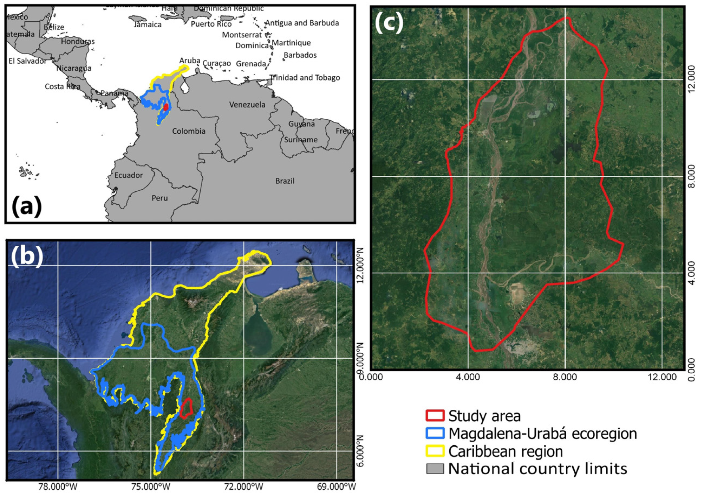
Our analysis was focused on a tropical seasonally flooded area that is part of the Magdalena-Urabá Moist forests [69]. The study area is also included in the Caribbean region, one of the five primary natural regions of the country identified by the Colombian environmental authorities [70] (Figure 1). Annual rainfall ranges from 2095 mm to 3119 mm throughout the study area. The rainy season is bimodal, with maximum rainfall from April to May and September to October; January and February are the driest months of the year [71]. The Magdalena River, the most important river in Colombia in terms of transportation, crosses the study area from south to north, forming seasonal wetlands where the water level changes through rainy and dry months. Land cover changes generated by human influence, such as deforestation and the draining of wetlands, have generated mosaics of native forests, wetlands, and land cover of anthropic origin in the study area.

2.2. Response Variables and Sample Data

We used two sets of land cover legends as categorical response variables. (1) The first land cover legend was the CORINE second level, which is formed by ten classes (Table 1). In Colombia, CORINE is structured in five hierarchical levels where the first two levels are the most general and present the same land cover classes of Europe [25]. After assessing field observations and high spatial resolution imagery, we found that the land cover classes of the CORINE second level adjust better to represent the biophysical conditions of the study area than the other CORINE levels. (2) We also developed a second legend, termed ECOSO, tailored to the ECOlogical and SOcioeconomic conditions of the study area. The ECOSO legend consists of eight classes representing the three main natural covers of the study area, moist forest, wetlands, and areas dominated by natural herbs and shrubs. We represented the primary agricultural activities in the study area with two classes: palm plantations and grassland, the latter of which is used for cattle grazing. We divided palm plantations into young and mature classes because the field surveys of some animal taxa (insects, birds, and mammals) have shown differences in diversity and composition when these two palm plantation ages are sampled. The definitions of each land cover of ECOSO are presented in Table 1.

To obtain the sample data, the study area was divided into square sample areas of 10 m × 10 m that match the Sentinel imagery pixel size. We then visually identified and selected the square sample areas with 100% of any of the land cover classes of the two legends for the year 2020, using the Google Satellite Plugin of QGIS 3.4 Madeira. As with other GIS applications (e.g., Google Earth and the Basemap of ArcGIS), the Madeira Plugin grants the visualization of high spatial resolution imagery (e.g., WorldView, Ikonos, QuickBird, and GeoEye) to experienced analysts who later select ideal areas of each land cover [40,64,65]. We randomly selected 49,500 of these square sample areas as sample data, using a spatial filter of 20 m² to reduce spatial autocorrelation effects. We used a sample size of 49,500 because it was the sample size where classification algorithms started to achieve confident landcover classification (see land cover modeling section).

2.3. Predictor Variables

We built mosaics of temporal mean metrics using the pixel values of all imagery of Sentinel-1 (SAR data) and Sentinel-2 (multispectral data) available between 1 January 2020 and 31 December 2020 in the Google Earth Engine [37]. These mosaics were used as predictor variables and were built for the backscatter coefficients, bands, and indices of Table 2. These mosaics also were built for three different periods: (1) The annual mean using all imagery of 2020, (2) the dry-season mean using the imagery of the two driest months of 2020, and (3) the rainy-season mean using the imagery of the five rainiest months of the year.

To create the Sentinel-1 mosaics, we used the product Sentinel-1 SAR GRD (C-band Synthetic Aperture Radar Ground Range Detected) of Google Earth Engine-GEE [77]. This product provides calibrated and ortho-corrected Sentinel-1 data. We also applied an angular-based radiometric slope correction to this product [78], using the correction model used for vegetation covers and the ALOS Global Digital Surface Model (AW3D30) to estimate surface slope. To create the Sentinel-2 mosaics, we used the products Sentinel-2 MSI (Multispectral Instrument-Level-2A) [79] and Sentinel-2—Cloud Probability of GEE [80]. Sentinel-2 MSI provides the corrected BOA (Bottom Of Atmosphere) reflectance of the Sentinel-2 images. Sentinel-2—Cloud Probability provides information to mask pixels with a high probability of cloud using the LightGBM library. We combined these two Sentinel-2 products following Braaten (2022) for masking clouds and cloud shadows [81]. Clouds were identified from the Sentinel-2—Cloud Probability dataset and shadows are defined by a cloud projection intersection with low-reflectance near-infrared (NIR) pixels.

We also used two geomorphological auxiliary predictors generated from the ALOS Global Digital Surface Model (AW3D30), topographic slope and topographic position index (TPI) [82]. This type of geomorphological data is useful in assisting the mapping of wetlands because the landforms constrain the wetland distribution [27]. The topographic slope was defined as the degree of inclination between the surface normal and a horizontal plane. TPI is an index of terrain classification where the altitude of each pixel is evaluated against its neighborhood pixels. If a pixel is higher than its surroundings, the TPI will be positive, for instance on ridges and hilltops; TPI will be negative for low-lying pixels, such as those corresponding to valleys where wetlands are more common [27,83]. After evaluating the effects of the predictors on the land cover mapping, we excluded the TPI of the final modeling because the TPI did not affect the prediction of the land cover (see the section on land cover mapping).

2.4. Land Cover Discrimination by Temporal Mean Metrics

We selected 400 sample data per land cover of the CORINE and the ECOSO legend to perform one-way ANOVAS for evaluating the land cover classifications generated by the three temporal mean metrics (annual, dry-season, and rainy-season periods) of each SAR and multispectral datum. Significant differences would show that the backscatter coefficients, bands, or spectral indices behave differently depending on the period, providing support that metrics could be used as predictor variables to help to discriminate between land covers.

2.5. Land Cover Modeling

We modeled the land covers identified in the sample data as response variables and used their corresponding values of the three temporal mean metrics of Sentinel (Sentinel-1 and Sentinel-2) and the auxiliary data as predictor variables. This procedure was performed for both legends. We assessed five learning algorithms that apply to different statistical methods to predict the response variable: (1) Bootstrap aggregating trees or Bagging (BAG), (2) Random Forest (RF), (3) Linear support vector machine (SVM_L), (4) Radial support vector machine (SVM_R), and (5) Multivariate Adaptive Regression Splines (MARS). We tuned the parameters of the learning algorithms to achieve the most accurate predicted models following Boehmke and Greenwell (2019) [84]. We performed the learning algorithms in different sample sizes from 1500 to 49,500 (1500, 3000, 4500, …, and 49,500 data samples) using the R Package ‘caret’ [85]. We used the Overall Accuracy (OA) and Cohen’s kappa coefficient (kappa) estimated in five-cross validations (CV) to measure the accuracy of the models.

To compare the effect of the three types of temporal mean metrics (annual, dry-season, and rainy-season metrics) and the three types of remote sensing data (Sentinel-1, Sentinel-1, and geomorphological auxiliary) on the accuracy of the land cover classifications, we calculated the predictors’ importance for the learning algorithms at a sample size of 49,500 sample data using the R package caret [85]. This package applies the methods of each learning algorithm to estimate predictor importance and scales the maximum importance to the value of 100, allowing the comparison of the importance among different algorithms. For BAG and RF classifications, the prediction accuracy of the out-of-bag portion of the data is recorded for each tree. Then, the same is repeated after permuting each predictor variable. The difference between the two accuracies is then averaged over all trees and normalized by the standard error [85,86]. For MARS, a backward elimination feature selection routine that looks at reductions in the generalized cross-validation estimate of error is performed. The function tracks the changes in model statistics for each predictor and accumulates the reduction in the statistic when each predictor’s feature is added to the model. This total reduction is used as the variable importance measure [87]. SVM_L and SVM_R lack a reliable methodology to estimate the importance of the predictors.

2.6. Land Cover Mapping

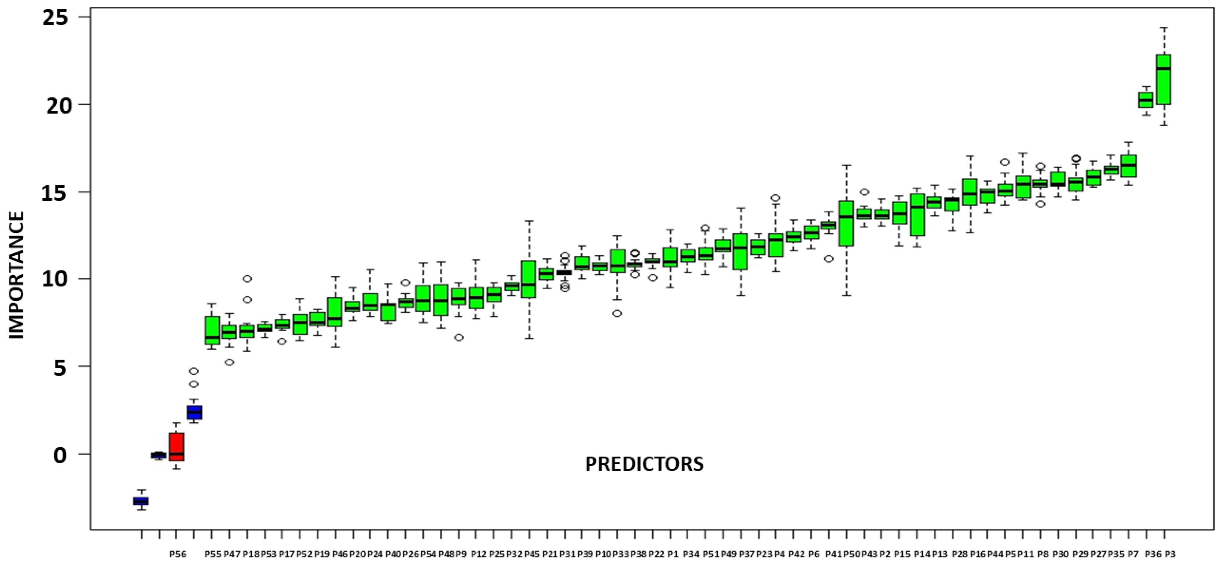
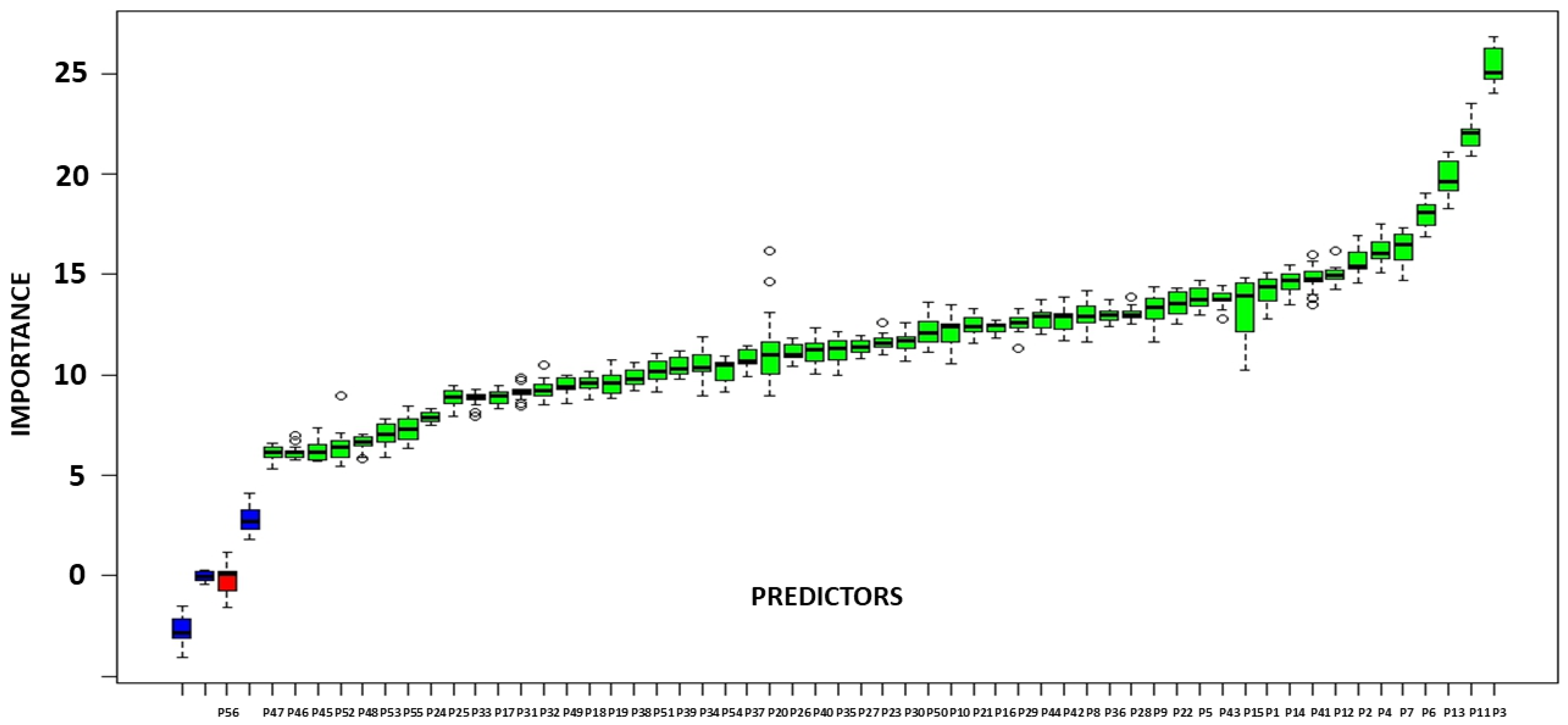
We generated land cover maps for the CORINE and ECOSO legends using the learning algorithm that produced the highest accuracy measures using the previous modeling of the sample data. Before the creation of these maps, we performed a Boruta analysis [88] to identify the importance of the predictors on the land cover modeling and eliminate possible predictors with no importance. The Boruta algorithm compares predictor importance with shadow predictors (predictor copies generated by random permutations of their own values) in numerous classifications, 100 in our case. Predictors with a significantly larger or smaller importance than shadow predictors are declared as important or unimportant for the modeling. The result of the Boruta analyses showed that all the predictors, except TPI, presented significant effects on the modeling of the land cover for the ECOSO and CORINE legends (Figure A1 and Figure A2). Therefore, the final modeling excluded TPI.

We then measured map accuracies by estimations of OA and kappa, using the predicted land covers of the maps against the validation data obtained from 2131 field surveys. We also estimated sensitivity (the proportion of testing data of a land cover correctly classified or true positive rate), specificity (the proportion of testing data of a land cover incorrectly classified as another land cover or true negative rate), and F1 score (the harmonic-mean of precision and recall for the minority positive class) to evaluate the accuracy of the classifications per land cover. These accuracy metrics were estimated for the CORINE and ECOSO legends by partitioning the sample data into training (70%) and testing (30%) sets.

3. Results

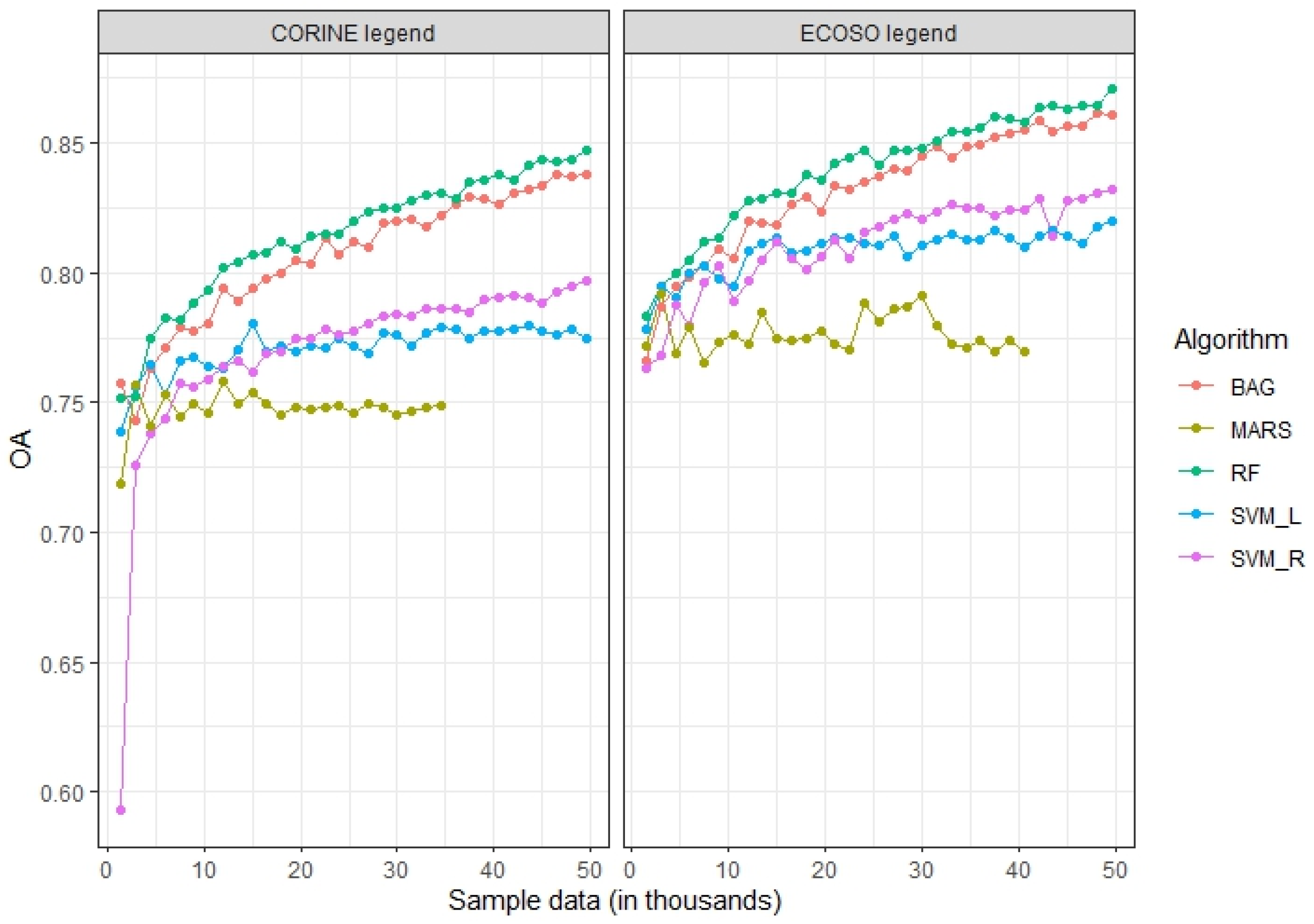
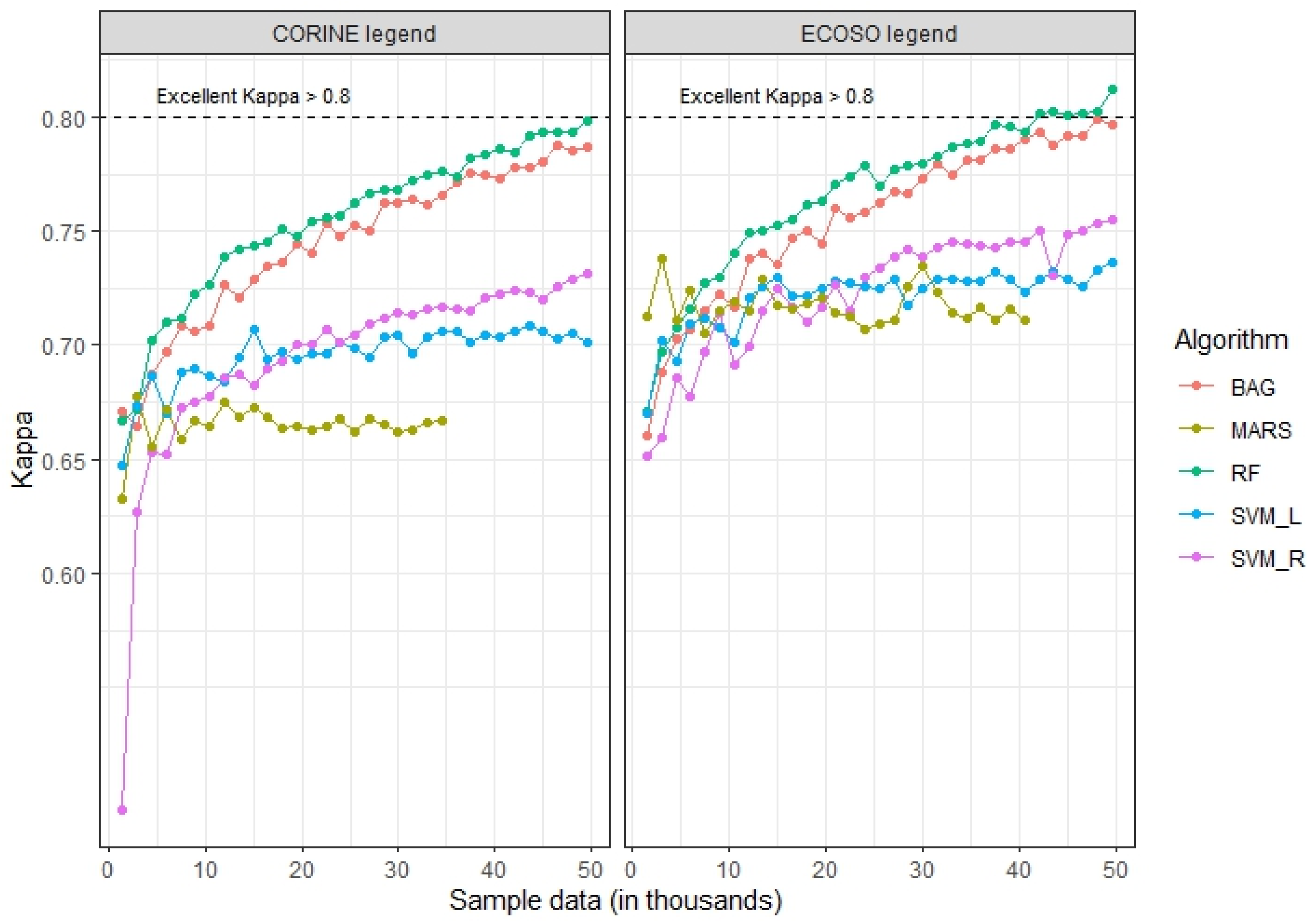
Five-cross validations showed that the learning algorithms used in the land cover modeling produced more accurate classifications when the land covers of the ECOSO legend were used as response variables compared with the CORINE legend for the different sample sizes evaluated (Paired T-Tests values: For OA; T > 10.02 and p-value < 0.001. For kappa; T > 7.1 and p-value < 0.001) (Figure 2 and Figure 3).

Most temporal means of the multispectral and SAR data showed significant differences in the same land cover when annual, dry-season, and rainy-season periods were compared for the ECOSO legend and CORINE legend (Table A1 and Table A2). The backscatter coefficients VV, VH, and VV—VH of Sentinel-1 and most bands and indices of Sentinel-2 were different within each land cover (p-value < 0.04; F = 3.06), excepting land cover corresponding to infrastructure and water bodies of the ECOSO legend. This also occurred within land cover corresponding to open areas with little or no vegetation, urban zones, and water bodies of the CORINE legend. The VV/VH backscatter ratio and the blue and green bands tended to present the lowest variations within each land cover.

The RF algorithm generated the most accurate models across the different sample sizes for both land cover legends, the ECOSO (paired T-test values: For OA; T > 11.82 and p-value < 0.001. For kappa; T > 6.22 and p-value < 0.001) and CORINE (paired T-test values: For OA; T > 10.72 and p-value < 0.001. For kappa; T > 10.62 and p-value < 0.001). We also found that only the RF algorithm generated excellent classifications (kappa > 0.8) for the land cover of the ECOSO legend when the sample size was over 42,000. No algorithms generated classifications with kappa > 0.8 for the CORINE legend (Figure 2 and Figure 3).

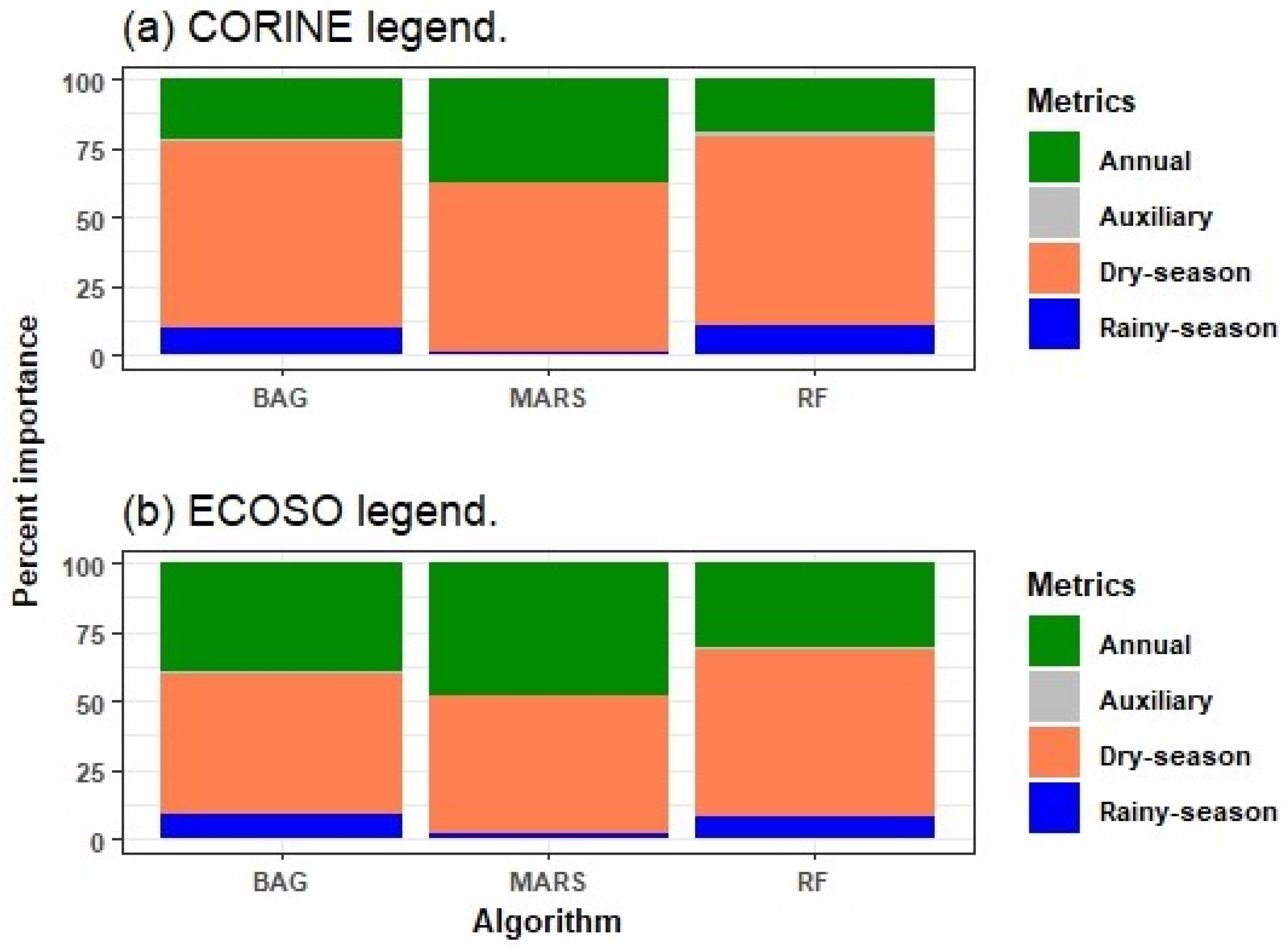
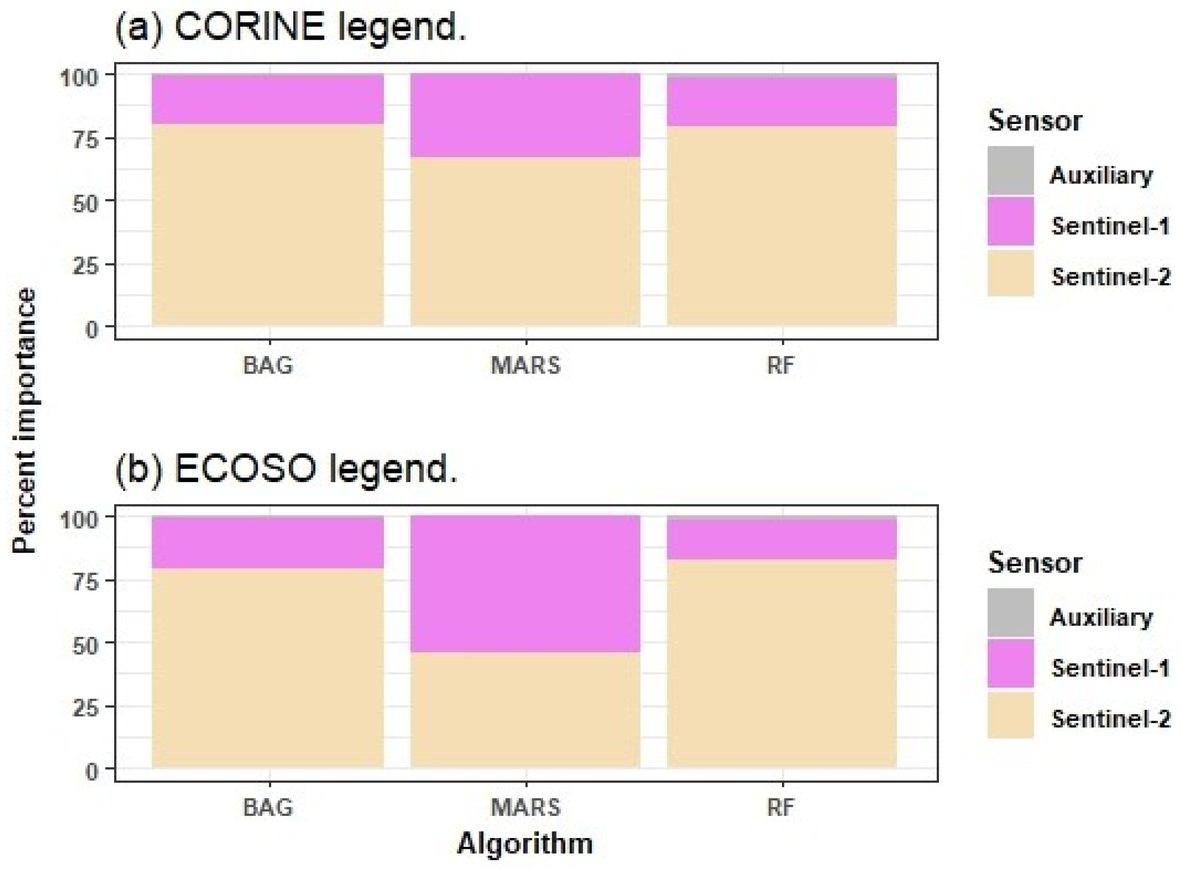
The predictor importance generated by the three types of temporal metrics varied for the ECOSO (X² = 10.38, df = 3, p-value = 0.01) and the CORINE (X² = 9.97, df = 3, p-value = 0.01) legends in the classifications generated by the BAG, RF, and MARS algorithms. Dry-season metrics presented the highest importance (~65%) compared with the annual (~37%) and rainy-season (~7.6%) metrics for both legends (ECOSO: Z > 2.03, p-value < 0.03; CORINE: Z > 2.15, p-value < 0.03) (Figure 4). In addition, the three types of remote sensing data showed different predictor importance for the ECOSO (X² = 6.48, df = 2, p-value = 0.03) and CORINE (X² = 7.2, df = 2, p-value = 0.02) legends in the three learning algorithms evaluated. Metrics generated by Sentinel-2 presented the highest importance (~75.1%) compared with the metrics generated by Sentinel-1 (~23.9%) and the geomorphological auxiliary metrics (~1%) for the ECOSO legends (Z > 2.53; p-value < 0.03) and CORINE (Z > 2.68; p-value < 0.01) legends (Z > 2.53; p-value < 0.03) (Figure 5).

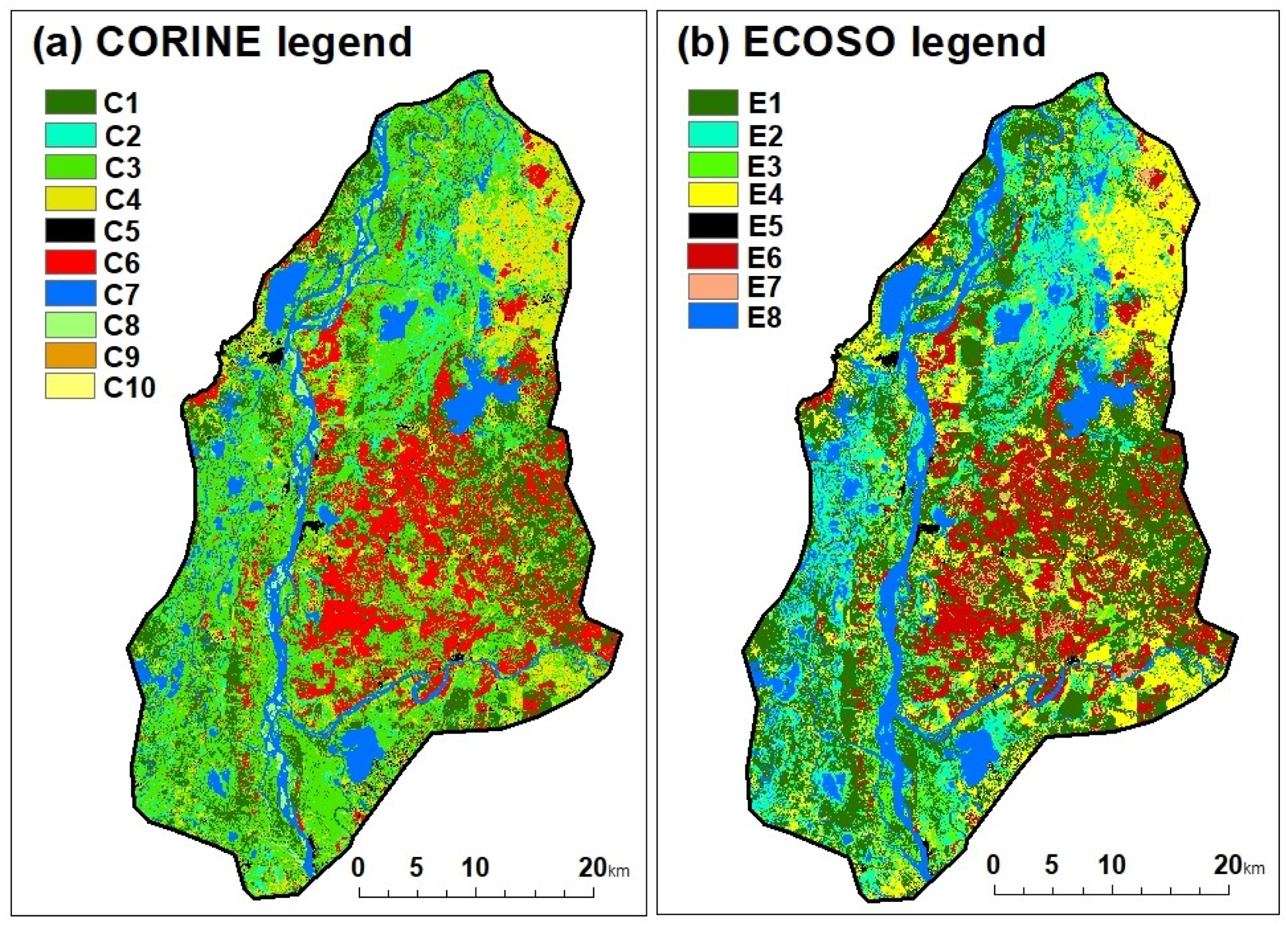
The map for the ECOSO legend obtained higher accuracy than the map for the CORINE legend when the OA (0.81 for the ECOSO Legend and 0.73 for the CORINE legend) and kappa (0.75 for the ECOSO legend and 0.61 for the CORINE legend) were estimated using the validation data obtained from surveys in the field (Figure 6). Herbaceous, grassland, and/or shrub vegetation for the CORINE legend and herbaceous, wetland, and shrubland for the ECOSO legend produced the lowest sensitivity values (0.60 < sensitivity < 0.66), indicating that these land cover classes are the most difficult to map. All land cover of both legends generated high values of specificity (>0.95), that is, the proportion of testing data of land cover incorrectly classified as a land cover was low in general terms. Moreover, the F1 scores were relatively low for heterogeneous agricultural areas (0.53) of the CORINE legend and herbaceous vegetation and shrubland (0.59) of the ECOSO legend (Table A3 and Table A4).

4. Discussion

By integrating dry-season, rainy-season, and annual metrics of SAR and multispectral data with visual pixel classifications and field surveys, we obtained high accuracies for land cover modeling (kappa < 0.82) and land cover mapping (kappa < 0.76) in a tropical region with seasonal flooding at a detailed spatial resolution (10 m). We used free and open-access data and software; therefore, our methods can be adopted in other regions to construct land cover maps. We highlight that our classification analyses were based on large sample data (Big data) that were performed in a high-performance computing cluster. This could be a limitation for the development of this type of analysis; however, desktop computers can perform classifications with enough data sizes to produce land cover maps with sufficiently high accuracy.

Previous studies on the land cover modeling of tropical regions have obtained lower accuracies at coarser spatial resolutions when annual metrics are used [14,89,90], demonstrating that the inclusion of more temporal metrics can increase the accuracy of land cover mapping. On the other hand, findings using the reflectance and backscatter values of individual SAR and multispectral images as well as smaller sample sizes of the sample data set (sample data < 200) showed higher accuracies for the land cover mapping of the tropical regions of Colombia (kappa > 0.86) [56]. Theoretically, temporal metrics should increase the resulting accuracies of the land cover modeling and land cover mapping due to the inclusion of the phenological characteristics of the vegetation [40,51,53]. Although differences in the terrain’s physical conditions and the landcover legends make it difficult to compare the resulting accuracies of different land cover mapping efforts, it is possible that a spatial bias or dependence between sample and validation data inflates map accuracies when only one image and low sample sizes are used [62,63]. To clarify this type of discrepancy, it is necessary to consistently evaluate the use of temporal metrics estimated from temporal stacks of imagery against the reflectance and textural metrics estimated from individual images.

The dry-season metrics estimated of SAR and multispectral data had higher importance in the land cover classifications than the rainy-season metrics. Some classes of the ECOSO and CORINE legends were built based on vegetation characteristics, and the dry season is a period of water stress for some of these vegetation types. Grassland, shrubland, and herbaceous vegetation are highly exposed to water limitations during the dry season, which significantly reduces their greenness and changes their structure (loss of leaves), while the forest and wetland vegetation are less exposed to such limitations and thus can maintain a relatively higher greenness and a higher leaf density. These phenological variations would maximize the spectral differences during the dry season among land cover types. On the other hand, during the rainy season, all vegetation types have less moisture limitation and higher photosynthesis levels and leaf density; consequently, their SAR and multispectral signatures may present similarities. These spectral similarities make it difficult to discriminate land cover classes when classification algorithms and remote sensing data are used in tropical environments [30,91,92]. Interestingly, the dry-season metrics estimated of SAR and multispectral data also had a higher importance in the land cover classifications than the annual metrics. Although annual metrics capture the spectral differences of the dry season, increasing land cover discrimination, annual metrics also capture the spectral similarities of the rainy season that reduce discrimination. This spectral ambiguity may explain why annual metrics were comparatively superior to rainy-season metrics but inferior to dry-season metrics for land cover classification.

Using the same reference dataset (sample data and predictor variables), we found that the land cover modeling and mapping for the ECOSO legend was more accurate than for the CORINE legend. The ECOSO legend included only land cover that represented the conditions of the study area while the CORINE legend contained a higher number of classes that are not well adapted to the study area, explaining its lower modeling and mapping accuracy. Some CORINE classes, such as heterogeneous agricultural areas and temporary crops, have ambiguous definitions for the study area and thus were difficult to discriminate by the learning algorithms, reducing the accuracy of the modeling and mapping. The ambiguous definition of some land cover is an issue frequently mentioned by technicians who build maps by the visual interpretation of high spatial resolution images when the CORINE legend is used in Colombia. We were able to detect the same issue in the land cover modeling of CORINE using learning algorithms.

We found lower differences in accuracy between the ECOSO and the CORINE legend for the land cover modeling (~2% for OA and ~1 for kappa values) than for the land cover mapping (8% for OA and 14 for kappa values). Previous authors have criticized the bias of land cover maps when accuracies are estimated only with partitions of the sample data (e.g., cross validations or data partitions) as we did with the accuracies of land cover modeling. These authors suggest that the non-independence of the data for estimating accuracies inflates OA and kappa due to variations of the prevalence generated by the high spatial correlation of sample data and human bias in imagery interpretation [63,93]. For those reasons, field confirmations of land cover maps prepared by accuracy estimations using surveys are essential to estimate more realistic OA and kappa values, as we did with the accuracies of the land cover mapping. The substantially lower OA and kappa for the land cover mapping of the CORINE compared to the ECOSO legend showed that the Random Forest modeling actually produced an inferior representation of the CORINE land cover.

The least accurately mapped land cover in both legends were the areas corresponding to herbaceous and shrub vegetation (C3 of the CORINE and L3 of the ECOSO legend in Table 1). Previous work has also encountered this issue from tropical to temporal environments [14,15,94,95]; these authors suggest that the performance classification of herbaceous and shrubland is relatively poor because their phenological changes produce greater intra-annual complexity and spectral variability than the other classes. We initially expected the classification of the wetland areas to be relatively poor due to their seasonal water-level changes that produce changes in their coverage areas during the same year. However, compared to previous works in other tropical regions [27,96], the wetland classifications for both legends (C2 of CORINE and L2 of the ECOSO legend in Table 1) presented higher accuracies. We demonstrated that the inclusion of seasonal predictors of SAR and multispectral data (dry-season, rainy-season, and annual metrics) and the topographic auxiliary predictor (topographic slope) reduced the errors of wetland classification; the former predictors involved the seasonal dynamic of the wetlands while the latter predictor discarded places where topography limits the wetland distribution.

After evaluating five learning algorithms with different statistical approaches to predict a response variable, we found that Random Forest was the best algorithm for our land cover modeling. Other works have also shown the better performance of Random Forest relative to other learning algorithms to predict land covers [97,98]. Although Random Forest requires some parameter tuning and predictor selection, the algorithm is relatively simple to use and is less affected by outliers, nonparametric data, and predictor correlation than other learning algorithms. Recently, deep learning algorithms (e.g., convolutional neural networks and deep learning networks) have shown competitive or superior accuracies to Random Forest for the modeling of land cover [99,100,101]; however, deep learning algorithms currently lack standardized methodologies to estimate the predictor importance which complicates inference related to the predictors.

The metrics generated by Sentinel-2 presented a higher importance for land cover modeling than the metrics generated by Sentinel-1 and the geomorphological auxiliary metrics in both evaluated land cover legends. A large number of Sentinel-2 predictors (42) compared with the Sentinel-1 (12) and geomorphological (1) predictors produced a higher general importance of Sentinel-2. However, the comparative importance of Sentinel-1 is not low (~23.9%), confirming that the integration of SAR (Sentinel-1) and multispectral (Sentinel-2) data is a suitable remote sensing strategy to improve land cover classifications. We also found that three Sentinel-1 predictors for the CORINE legend and one Sentinel-1 predictor for the ECOSO legend were among the most important ten predictors for the land cover classification of each legend, demonstrating the positive effect of this sensor in both land cover classifications.

5. Conclusions

We demonstrated that it is possible to improve land cover modeling by integrating the temporal metrics of SAR and multispectral data with visual pixel classifications and field surveys. The use of dry-season, rainy-season, and annual metrics of Sentinel-1 and Sentinel-2 captured the phenological and structural variation of the vegetation that comprises land cover, increasing land cover discrimination by typical learning algorithms used for modeling and mapping. We showed that these learning algorithms produced high accuracies for modeling and mapping when land cover legends were developed using the ecological and socioeconomic conditions of the study area. Conversely, accuracy estimations are lower when these learning algorithms model land cover legends developed for different contexts, as in the case of the CORINE legend adapted to Colombia. These results suggest the need to build an official land cover legend for Colombia using information on the environmental conditions of the country. Our results also confirm the importance of the independence between the sample and validation data to avoid inflating the accuracy estimation of the land cover maps. Future advances in remote sensing data and statistical methods are expected to increase the accuracy of the land cover maps generated by supervised classifications. However, the reliability of land cover legends in describing the characteristics of the regions and countries in which they are used will be a fundamental step to increasing these accuracies. For this reason, in countries such as Colombia, where the official legend has been transferred from other countries or regions, it is necessary to start thinking about the design of a national legend that brings together the country’s own regional variation and facilitates future planning.

Author Contributions

Conceptualization, J.C.F. and S.R.-B.; Methodology, J.C.F., S.R.-B. and P.J.; Formal analysis, J.C.F.; Investigation, J.C.F., S.R.-B. and P.J.; Resources, J.C.F. and S.R.-B.; Writing—review and editing, J.C.F., S.R.-B. and P.J. All authors have read and agreed to the published version of the manuscript.

Funding

This research was funded by the Agencia Nacional de hidrocarburos de Colombia and the Humboldt Institute, grant number 21-117-2020. Support for J.C.F. was provided by Universidad Nacional de Colombia—Sede Bogotá; Proyecto HERMES 58648 and Proyecto HERMES 52625. Support for P.J. was provided by NASA grants 80NSSC19K0186 and 80NSCC18K0338.

Data Availability Statement

Land cover maps that support the findings of this study will be openly available at the following URL/DOI: (https://doi.org/10.5281/zenodo.7799931).

Acknowledgments

We acknowledge Instituto Humboldt, Departamento de Biología of Universidad Nacional de Colombia (Sede Bogota D.C), and School of Informatics, Computing, and Cyber Systems of Northern Arizona University for providing technical support and data. This work is one of the requirements for the forgiveness of the COLCIENCIAS-loan 529-2011 for J.C.F.

Conflicts of Interest

The authors declare no conflict of interest.

Appendix A

Figure A1. Importance of predictors in the Random Forest classification for the land covers of the CORINE legend. Predictors with significant importance (green boxes), predictors with no significant importance (red boxes), and the maximum, minimum, and average of the shadow predictors (blue boxes). P1 (annual VV), P2 (annual VH), P3 (annual VH/VV), P4 (annual VH-VV), P5 (dry VV), P6 (dry VH), P7 (dry VH/VV), P8 (dry VH-VV), P9 (rainy VV), P10 (rainy VH), P11 (rainy VH/VV), P12 (rainy VH-VV), P13 (annual blue), P14 (annual green), P15 (annual red), P16 (annual red edge 1), P17 (annual red edge 2), P18 (annual red edge 3), P19 (annual near infrared), P20 (annual red edge 4), P21 (annual short wave infrared 1), P22 (annual short wave infrared 2), P23 (annual NDVI), P24 (annual EVI), P25 (annual SAVI), P26 (annual RNDVI), P27 (dry blue), P28 (gry green), P29 (dry red), P30 (dry red edge 1), P31 (dry red edge 2), P32 (dry red edge 3), P33 (dry near infrared), P34 (dry red edge 4), P35 (dry short wave infrared 1), P36 (dry short wave infrared 2), P37 (dry NDVI), P38 (dry EVI), P39 (dry SAVI), P40 (dry RNDVI), P41 (rainy blue), P42 (rainy green), P43 (rainy red), P44 (rainy red edge 1), P45 (rainy red edge 2), P46 (rainy red edge 3), P47 (rainy near infrared), P48 (rainy red edge 4), P49 (rainy short wave infrared 1), P50 (rainy short wave infrared 2), P51 (rainy NDVI), P52 (rainy EVI), P53 (rainy SAVI), P54 (rainy RNDVI), P55 (slope), and P56 (TPI).

Appendix B

Figure A2. Importance of predictors in the Random Forest classification for the land covers of the ECOSO legend. Predictors with significant importance (green boxes), predictors with no significant importance (red boxes), and the maximum, minimum, and average of the shadow predictors (blue boxes). P1 (annual VV), P2 (annual VH), P3 (annual VH/VV), P4 (annual VH-VV), P5 (dry VV), P6 (dry VH), P7 (dry VH/VV), P8 (dry VH-VV), P9 (rainy VV), P10 (rainy VH), P11 (rainy VH/VV), P12 (rainy VH-VV), P13 (annual blue), P14 (annual green), P15 (annual red), P16 (annual red edge 1), P17 (annual red edge 2), P18 (annual red edge 3), P19 (annual near infrared), P20 (annual red edge 4), P21 (annual short wave infrared 1), P22 (annual short wave infrared 2), P23 (annual NDVI), P24 (annual EVI),P25 (annual SAVI), P26 (annual RNDVI), P27 (dry blue), P28 (dry green), P29 (dry red), P30 (dry red edge 1), P31 (dry red edge 2), P32 (dry red edge 3), P33 (dry near infrared), P34 (dry red edge 4), P35 (dry short wave infrared 1), P36 (dry short wave infrared 2), P37 (dry NDVI), P38 (dry EVI), P39 (dry SAVI), P40 (dry RNDVI), P41 (rainy blue), P42 (rainy green), P43 (rainy red), P44 (rainy red edge 1), P45 (rainy red edge 2), P46 (rainy red edge 3), P47 (rainy near infrared), P48 (rainy red edge 4), P49 (rainy short wave infrared 1), P50 (rainy short wave infrared 2), P51 (rainy NDVI), P52 (rainy EVI), P53 (rainy SAVI), P54 (rainy RNDVI), P55 (slope), and P56 (TPI).

Appendix C

Table A1. Summary of one-way ANOVAS to compare the temporal mean values of the multispectral and SAR data per land cover of the ECOSO legend for three periods of 2020: (1) Annual mean using all imagery of 2020; (2) dry season mean using the imagery of the two driest months of 2020; and (3) rain season mean using the imagery of the five rainiest months of the year. We found significant differences among these three periods that show that the temporal means per band, multispectral index, and backscatter coefficient behave differently during the evaluated periods. These differences demonstrate that the temporal mean value calculated for each of these periods can be used as a variable to discriminate land covers in the study area. The first letter and second letter in the SAR data (H or V) refer to the transmit and return signals; H stands for horizontal and V for vertical polarizations. Significant p values range; p < 0.001 (***), p < 0.01 (**), and p < 0.05 (*).

Satellite (Data Type)	Band, Index Name, or Backscatter Coefficient	Land Cover Class	F-Value	p-Value	Significance
	VV	Tropical moist forest	6	0.002568297	**
		Grassland	62	3.67405E-26	***
		Herbaceous and shrubland	23	1.57724E-10	***
		Infrastructure	0	0.631883799
		Mature palm plantations	72	3.08908E-30	**
		Water	3	0.031589942	*
		Wetland	11	1.76326E-05	***
		Young palm plantations	90	3.55004E-37	***
	VH	Tropical moist forest	6	0.002387089	**
		Grassland	84	4.77421E-35	***
		Herbaceous and shrubland	26	1.27439E-11	***
		Infrastructure	1	0.343709726
		Mature palm plantations	139	5.1437E-55	***
		Water	7	0.000870292	***
		Wetland	3	0.053333071	*
		Young palm plantations	101	3.48339E-41	***
	VVmVH	Tropical moist forest	5	0.008475596	**
		Grassland	47	3.22066E-20	***
		Herbaceous and shrubland	18	2.72475E-08	***
		Infrastructure	0	0.680842298
		Mature palm plantations	42	1.51053E-18	***
		Shrubland	8	0.000320566	***
		Water	2	0.090936068
		Wetland	14	1.33331E-06	***
		Young palm plantations	62	1.71158E-26	***
	VHdVV	Tropical moist forest	1	0.297645719
		Grassland	0	0.645580222
		Herbaceous and shrubland	0	0.846826805
		Infrastructure	0	0.977296257
		Mature palm plantations	9	0.000140432	***
		Water	0	0.760810131
		Wetland	11	2.46617E-05	***
		Young palm plantations	3	0.040476133	*
	BLUE	Tropical moist forest	2	0.153644537
		Grassland	5	0.00609176	*
		Herbaceous and shrubland	2	0.12682676
		Infrastructure	5	0.004748278	*
		Mature palm plantations	42	3.40328E-18	***
		Water	7	0.001516881	*
		Wetland	11	2.93761E-05	***
		Young palm plantations	29	4.75329E-13	***
	GREEN	Tropical moist forest	3	0.053247018	*
		Grassland	2	0.132665756
		Herbaceous and shrubland	2	0.207288516
		Infrastructure	7	0.001213031	**
		Mature palm plantations	4	0.017734227	*
		Water	1	0.225658337
		Wetland	6	0.003982018	**
		Young palm plantations	2	0.115107982
	RED	Tropical moist forest	5	0.010667312	*
		Grassland	17	5.21408E-08	***
		Herbaceous and shrubland	6	0.002036325	*
		Infrastructure	3	0.046986096	*
		Mature palm plantations	56	6.96644E-24	***
		Water	4	0.012729719	*
		Wetland	23	2.33559E-10	***
		Young palm plantations	44	2.82816E-19	***
	RED_E_1	Tropical moist forest	11	1.62602E-05	***
		Grassland	2	0.216948004
		Herbaceous and shrubland	3	0.033364352	*
		Infrastructure	10	6.81317E-05	***
		Mature palm plantations	3	0.038285219	*
		Water	8	0.00024883	***
		Wetland	11	1.72503E-05	***
		Young palm plantations	2	0.164089184
	RED_E_2	Tropical moist forest	110	1.25924E-44	***
		Grassland	113	7.53722E-46	***
		Herbaceous and shrubland	38	8.18867E-17	***
		Infrastructure	18	1.79485E-08	***
		Mature palm plantations	410	2.3864E-136	***
		Water	4	0.020459247	*
		Wetland	14	6.56859E-07	***
		Young palm plantations	341	6.1106E-118	***
	RED_E_3	Tropical moist forest	114	6.74092E-46	***
		Grassland	113	1.40749E-45	***
		Herbaceous and shrubland	37	2.16841E-16	***
		Infrastructure	18	2.92979E-08	***
		Mature palm plantations	423	1.76E-139	***
		Water	4	0.016013878	*
		Wetland	16	1.78503E-07	***
		Young palm plantations	333	8.7789E-116	***
	NIR	Tropical moist forest	65	1.81645E-27	***
		Grassland	63	1.16778E-26	***
		Herbaceous and shrubland	21	9.85588E-10	***
		Infrastructure	9	0.000172513	***
		Mature palm plantations	291	1.5266E-103	***
		Water	3	0.056042942	*
		Wetland	10	5.68407E-05	***
		Young palm plantations	236	5.56687E-87	***
	RED_E_4	Tropical moist forest	95	4.88148E-39	***
		Grassland	77	2.82783E-32	***
		Herbaceous and shrubland	29	4.25091E-13	***
		Infrastructure	15	2.53381E-07	***
		Mature palm plantations	388	1.926E-130	***
		Water	3	0.059911938	*
		Wetland	11	1.26172E-05	***
		Young palm plantations	291	1.5251E-103	***
SWIR_1	Tropical moist forest	13	3.99272E-06	***
	Grassland	38	1.44193E-16	***
	Herbaceous and shrubland	6	0.002912467	**
	Infrastructure	10	5.48921E-05	***
	Mature palm plantations	8	0.000514043	**
	Water	3	0.043625139	*
	Wetland	30	2.57828E-13	***
	Young palm plantations	13	3.20698E-06	***
SWIR_2	Tropical moist forest	2	0.187005907
	Grassland	42	1.53557E-18	***
	Herbaceous and shrubland	8	0.000266878	***
	Infrastructure	6	0.00235001	**
	Mature palm plantations	7	0.001428365	**
	Water	8	0.000312134	**
	Wetland	37	3.01375E-16	***
	Young palm plantations	26	6.6958E-12	***
EVI	Tropical moist forest	50	1.03023E-21	***
	Grassland	58	1.03682E-24	***
	Herbaceous and shrubland	17	3.80441E-08	***
	Infrastructure	2	0.207651799
	Mature palm plantations	276	2.9126E-99	***
	Water	1	0.449498764
	Wetland	11	2.70347E-05	***
	Young palm plantations	186	4.50887E-71	***
SAVI	Tropical moist sorest	41	4.27621E-18	***
	Grassland	45	1.15582E-19	***
	Herbaceous and shrubland	14	7.42276E-07	***
	Infrastructure	1	0.384579741
	Mature palm plantations	260	2.23105E-94	***
	Water	0	0.739025492
	Wetland	8	0.000341478	**
	Young palm plantations	175	2.39727E-67	***
RNDVI	Tropical moist forest	5	0.009506599	**
	Grassland	32	4.23285E-14	***
	Herbaceous and shrubland	11	1.7484E-05	***
	Infrastructure	6	0.003625327	**
	Mature palm plantations	3	0.034660805	*
	Water	3	0.043060708	*
	Wetland	13	2.06961E-06	***
	Young palm plantations	6	0.00176677	**
NDVI	Tropical moist forest	14	7.66839E-07	***
	Grassland	25	2.5465E-11	***
	Herbaceous and shrubland	8	0.000231118	**
	Infrastructure	0	0.858098151
	Mature palm plantations	142	6.91379E-56	***
	Water	1	0.493770717
	Wetland	3	0.046984903	*
	Young palm plantations	92	8.82396E-38	***

Appendix D. (Long Table, It Was Added after References)

Table A2. Summary of one-way ANOVAS to compare the temporal mean values of the multispectral and SAR data per land cover of the CORINE legend for three periods of 2020: (1) Annual mean using all imagery of 2020; (2) Dry season mean using the imagery of the two driest months of 2020; and (3) Rain season mean using the imagery of the five rainiest months of the year. We found significant differences among these three periods that show that the temporal means per band, multispectral index, and backscatter coefficient behave differently during the evaluated periods. These differences demonstrate that each temporal mean value calculated for these periods can be used as a variable to discriminate land covers in the study area. The first letter and second letter in the SAR data (H or V) refer to the transmit and return signals; H stand for horizontal and V for vertical polarizations. Significant p values range; p < 0.001 (***), p < 0.01 (**), and p < 0.05 (*).

Satellite (Data Type)	Band, Index Name, or Backscatter Coefficient	Land Cover Class	F-Value	p-Value	Significance
Sentinel-1 (SAR)	VV	Urban areas	3.8	0.022657	*
		Temporary crops	77.9	1.57E-32	***
		Permanent crops	34.5	2.61E-15	***
		Grassland	33.0	1.1E-14	***
		Heterogeneous agricultural areas	149.5	1.1E-58	***
		Forest	9.8	5.93E-05	***
		Areas with herbaceous and/or shrub vegetation	7.0	0.000905	***
		Open areas with little or no vegetation	1.7	0.182592
		Continental humid areas	41.8	2.82E-18	***
		Water	1.9	0.151496
	VH	Urban areas	2.5	0.080392
		Temporary crops	157.8	1.55E-61	***
		Permanent crops	62.9	1.08E-26	***
		Grassland	51.8	2.66E-22	***
		Heterogeneous agricultural areas	386.7	2.9E-130	***
		Forest	8.3	0.000261	***
		Areas with herbaceous and/or shrub vegetation	7.4	0.000615	***
		Open areas with little or no vegetation	22.7	2.11E-10	***
		Continental humid areas	9.5	8E-05	***
		Water	4.3	0.014194	**
	VVmVH	Urban areas	3.8	0.023579	*
		Temporary crops	57.3	1.77E-24	***
		Permanent crops	19.3	5.67E-09	***
		Grassland	23.2	1.26E-10	***
		Heterogeneous agricultural areas	71.5	4.72E-30	***
		Forest	8.6	0.000187	***
		Areas with herbaceous and/or shrub vegetation	5.7	0.003311	*
		Open areas with little or no vegetation	0.0	0.98551
		Continental humid areas	50.6	7.73E-22	***
		Water	1.3	0.279511
	VHdVV	Urban areas	2.9	0.058313
		Temporary crops	0.4	0.694037
		Permanent crops	3.4	0.032289	*
		Grassland	3.2	0.041195	*
		Heterogeneous agricultural areas	6.8	0.001139	*
		Forest	2.5	0.07944
		Areas with herbaceous and/or shrub vegetation	1.5	0.221896
		Open areas with little or no vegetation	188.8	5.28E-72	***
		Continental humid areas	15.3	2.66E-07	***
		Water	0.7	0.514729
Sentinel-2 (Multispectral)	BLUE	Urban areas	1.0	0.352686
		Temporary crops	1.0	0.351463
		Permanent crops	21.2	9.04E-10	***
		Grassland	10.9	2.06E-05	***
		Heterogeneous agricultural areas	4.0	0.018951	*
		Forest	10.1	4.43E-05	***
		Areas with herbaceous and/or shrub vegetation	1.5	0.232523
		Open areas with little or no vegetation	281.4	7E-101	***
		Continental humid areas	24.2	5.18E-11	***
		Water	14.8	4.53E-07	***
	GREEN	Urban areas	1.1	0.323845
		Temporary crops	4.0	0.018853	*
		Permanent crops	1.1	0.342954
		Grassland	3.3	0.036229	*
		Heterogeneous agricultural areas	43.3	6.89E-19	***
		Forest	0.3	0.722477
		Areas with herbaceous and/or shrub vegetation	2.2	0.110736
		Open areas with little or no vegetation	278.3	5.7E-100	***
		Continental humid areas	6.7	0.001316	*
		Water	14.8	4.31E-07	***
	RED	Urban areas	0.2	0.855469
		Temporary crops	6.3	0.001832	**
		Permanent crops	17.2	4.15E-08	***
		Grassland	34.5	2.75E-15	***
		Heterogeneous agricultural areas	19.8	3.45E-09	***
		Forest	12.1	6.19E-06	***
		Areas with herbaceous and/or shrub vegetation	5.2	0.005423	*
		Open areas with little or no vegetation	213.5	5.11E-80	***
		Continental humid areas	73.6	7.3E-31	***
		Water	36.6	3.91E-16	***
	RED_E_1	Urban areas	0.6	0.568254
		Temporary crops	8.8	0.000166	***
		Permanent crops	13.9	1.07E-06	***
		Grassland	5.0	0.006749	*
		Heterogeneous agricultural areas	50.8	6.9E-22	***
		Forest	5.0	0.006819	*
		Areas with herbaceous and/or shrub vegetation	6.1	0.002329	*
		Open areas with little or no vegetation	204.9	3.01E-77	***
		Continental humid areas	16.7	7.11E-08	***
		Water	55.4	9.94E-24	***
	RED_E_2	Urban areas	28.0	2.16E-12	***
		Temporary crops	238.3	7.46E-88	***
		Permanent crops	166.7	1.38E-64	***
		Grassland	135.6	8.32E-54	***
		Heterogeneous agricultural areas	166.1	2.22E-64	***
		Forest	66.2	5.19E-28	***
		Areas with herbaceous and/or shrub vegetation	24.3	4.69E-11	***
		Open areas with little or no vegetation	33.0	1.16E-14	***
		Continental humid areas	34.0	4.49E-15	***
		Water	8.9	0.00014	*
	RED_E_3	Urban areas	23.3	1.7E-10	***
		Temporary crops	285.3	4.7E-102	***
		Permanent crops	143.5	1.36E-56	***
		Grassland	137.9	1.25E-54	***
		Heterogeneous agricultural areas	189.4	3.55E-72	***
		Forest	75.5	1.34E-31	***
		Areas with herbaceous and/or shrub vegetation	24.6	3.42E-11	***
		Open areas with little or no vegetation	21.5	6.91E-10	***
		Continental humid areas	40.7	7.86E-18	***
		Water	7.6	0.000514	**
	NIR	Urban areas	6.1	0.00236595	*
		Temporary crops	211.6	2.0775E-79	***
		Permanent crops	70.3	1.348E-29	***
		Grassland	74.0	4.8769E-31	***
Heterogeneous agricultural areas		107.5	1.1997E-43	***
Forest		46.1	4.9883E-20	***
Areas with herbaceous and/or shrub vegetation		14.6	5.2772E-07	***
Open areas with little or no vegetation		23.9	6.8998E-11	***
Continental humid areas		22.2	3.4788E-10	***
Water		5.4	0.00482082	*
RED_E_4	Urban areas	14.0	1.13E-06	***
	Temporary crops	283.1	2.1E-101	***
	Permanent crops	120.8	1.62E-48	***
	Grassland	101.1	2.77E-41	***
	Heterogeneous agricultural areas	147.3	6.28E-58	***
	Forest	63.1	8.5E-27	***
	Areas with herbaceous and/or shrub vegetation	17.6	2.98E-08	***
	Open areas with little or no vegetation	24.0	6.21E-11	***
	Continental humid areas	25.0	2.29E-11	***
	Water	5.8	0.003018	*
SWIR_1	Urban areas	15.2	3.47E-07	***
	Temporary crops	4.0	0.017824	*
	Permanent crops	13.7	1.27E-06	***
	Grassland	46.3	4.21E-20	***
	Heterogeneous agricultural areas	4.6	0.01007	*
	Forest	7.7	0.000479	**
	Areas with herbaceous and/or shrub vegetation	7.0	0.000932	**
	Open areas with little or no vegetation	253.7	1.41E-92	***
	Continental humid areas	32.4	1.94E-14	***
	Water	0.2	0.822389
SWIR_2	Urban areas	12.9	3.21E-06	***
	Temporary crops	4.9	0.007743	*
	Permanent crops	3.4	0.032219	*
	Grassland	60.9	6.76E-26	***
	Heterogeneous agricultural areas	16.9	5.65E-08	***
	Forest	1.7	0.182995
	Areas with herbaceous and/or shrub vegetation	8.0	0.000366	*
	Open areas with little or no vegetation	384.5	1.1E-129	***
	Continental humid areas	50.8	6.87E-22	***
	Water	0.6	0.568736
EVI	Urban areas	1.4	0.236922
	Temporary crops	122.9	2.92E-49	***
	Permanent crops	56.1	4.96E-24	***
	Grassland	81.5	6.47E-34	***
	Heterogeneous agricultural areas	99.1	1.51E-40	***
	Forest	39.0	3.9E-17	***
	Areas with herbaceous and/or shrub vegetation	10.5	2.97E-05	***
	Open areas with little or no vegetation	1.4	0.241734
	Continental humid areas	39.2	3.24E-17	***
	Water	0.1	0.877852
SAVI	Urban areas	0.9	0.400928
	Temporary crops	95.4	3.73E-39	***
	Permanent crops	55.1	1.3E-23	***
	Grassland	66.6	3.65E-28	***
	Heterogeneous agricultural areas	70.6	1.02E-29	***
	Forest	35.1	1.53E-15	***
	Areas with herbaceous and/or shrub vegetation	7.3	0.000692	**
	Open areas with little or no vegetation	1.1	0.347356
	Continental humid areas	28.3	9.89E-13	***
	Water	0.1	0.914428
	Urban areas	0.9	0.400928
RNDVI	Urban areas	3.6	0.027078146	*
	Temporary crops	2.2	0.108978781
	Permanent crops	17.3	4.06165E-08	***
	Grassland	17.9	2.11557E-08	***
	Heterogeneous agricultural areas	2.1	0.118146032
	Forest	6.7	0.001281665	**
	Areas with herbaceous and/or shrub vegetation	10.8	2.19194E-05	***
	Open areas with little or no vegetation	8.4	0.000228264	*
	Continental humid areas	8.7	0.000170631	**
	Water	5.8	0.003089327	**
NDVI	Urban areas	0.5	0.579018
	Temporary crops	30.7	1.03E-13	***
	Permanent crops	31.2	6.18E-14	***
	Grassland	40.5	9.95E-18	***
	Heterogeneous agricultural areas	31.5	4.58E-14	***
	Forest	11.4	1.27E-05	***
	Areas with herbaceous and/or shrub vegetation	1.7	0.191762
	Open areas with little or no vegetation	0.4	0.692677
	Continental humid areas	15.4	2.47E-07	***
	Water	1.1	0.335542

Appendix E

Table A3. Estimates of sensitivity (true positive rate) and specificity (true negative rate) for the CORINE landcover legend. Sensitivity and specificity were estimated by performing data partitions of the 49,500 sample data (training 70% and testing 30%).

Land Cover	Sensitivity	Specificity	F1 Score	Prevalence
Forest (C1)	0.72	0.96	0.68	0.09
Continental humid areas(C2)	0.74	0.97	0.60	0.04
Areas with herbaceous and/or shrub vegetation (C3)	0.62	0.95	0.69	0.22
Grassland (C4)	0.66	0.97	0.61	0.05
Urban areas (C5)	0.90	1.00	0.87	0.02
Permanent crops (C6)	0.83	0.98	0.82	0.09
Water (C7)	0.95	0.98	0.96	0.43
Temporary crops (C8)	0.93	1.00	0.71	0.00
Heterogeneous agricultural areas (C9)	0.82	1.00	0.53	0.00
Open areas with little or no vegetation (C10)	0.88	0.98	0.84	0.07

Appendix F

Table A4. Estimates of sensitivity (true positive rate) and specificity (true negative rate) for the ECOSO land cover legend. Sensitivity and specificity were estimated by performing data partitions of the 49,500 sample data (training 70% and testing 30%).

Land Cover	Sensitivity	Specificity	F1 Score	Prevalence
Tropical moist forest (L1):	0.75	0.97	0.78	0.15
Wetland (L2):	0.66	0.97	0.70	0.12
Herbaceous and shrubland (L3):	0.60	0.95	0.59	0.09
Grassland (L4):	0.72	0.98	0.66	0.05
Infrastructure (L5):	1.00	1.00	0.78	0.01
Mature palm plantations (L6):	0.83	0.98	0.78	0.05
Young palm plantations (L7):	0.77	0.99	0.71	0.03
Water (L8):	0.97	0.97	0.97	0.51

References

Winkler, K.; Fuchs, R.; Rounsevell, M.; Herold, M. Global land use changes are four times greater than previously estimated. Nat. Commun. 2021, 12, 2501. [Google Scholar] [CrossRef] [PubMed]
Rudel, T.K.; Coomes, O.T.; Moran, E.; Achard, F.; Angelsen, A.; Xu, J.C.; Lambin, E. Forest transitions: Towards a global understanding of land use change. Glob. Environ. Chang. Policy Dimens. 2005, 15, 23–31. [Google Scholar] [CrossRef]
Turner, B.L.; Lambin, E.F.; Reenberg, A. The emergence of land change science for global environmental change and sustainability. Proc. Natl. Acad. Sci. USA 2007, 104, 20666–20671. [Google Scholar] [CrossRef]
Song, X.P.; Hansen, M.C.; Stehman, S.V.; Potapov, P.V.; Tyukavina, A.; Vermote, E.F.; Townshend, J.R. Global land change from 1982 to 2016. Nature 2018, 560, 639. [Google Scholar] [CrossRef] [PubMed]
Friedlingstein, P.; Jones, M.W.; O’Sullivan, M.; Andrew, R.M.; Bakker, D.C.E.; Hauck, J.; Le Quéré, C.; Peters, G.P.; Peters, W.; Pongratz, J.; et al. Global Carbon Budget 2021. Earth Syst. Sci. Data Discuss. 2021, 2021, 1–191. [Google Scholar] [CrossRef]
Powers, R.P.; Jetz, W. Global habitat loss and extinction risk of terrestrial vertebrates under future land-use-change scenarios. Nat. Clim. Chang. 2019, 9, 323–329. [Google Scholar] [CrossRef]
Venter, Z.S.; Sydenham, M.A.K. Continental-Scale Land Cover Mapping at 10 m Resolution Over Europe (ELC10). Remote Sens. 2021, 13, 2301. [Google Scholar] [CrossRef]
Tulbure, M.G.; Hostert, P.; Kuemmerle, T.; Broich, M. Regional matters: On the usefulness of regional land-cover datasets in times of global change. Remote Sens. Ecol. Conserv. 2022, 8, 272–283. [Google Scholar] [CrossRef]
Cihlar, J. Land cover mapping of large areas from satellites: Status and research priorities. Int. J. Remote Sens. 2000, 21, 1093–1114. [Google Scholar] [CrossRef]
Congalton, R.G.; Gu, J.; Yadav, K.; Thenkabail, P.S.; Ozdogan, M. Global land cover mapping: A review and uncertainty analysis. Remote Sens. 2014, 6, 12070–12093. [Google Scholar] [CrossRef]
Vancutsem, C.; Achard, F.; Pekel, J.F.; Vieilledent, G.; Carboni, S.; Simonetti, D.; Gallego, J.; Aragão, L.E.O.C.; Nasi, R. Long-term (1990–2019) monitoring of forest cover changes in the humid tropics. Sci. Adv. 2022, 7, eabe1603. [Google Scholar] [CrossRef]
NASA. Land-Cover and Land-Use Change (LCLUC) Program. Available online: https://lcluc.umd.edu/ (accessed on 23 February 2023).
ESA. Land Cover Project. Available online: https://climate.esa.int/en/projects/land-cover/ (accessed on 23 February 2023).
Buchhorn, M.; Lesiv, M.; Tsendbazar, N.-E.; Herold, M.; Bertels, L.; Smets, B. Copernicus Global Land Cover Layers—Collection 2. Remote Sens. 2020, 12, 1044. [Google Scholar] [CrossRef]
Tsendbazar, N.E.; de Bruin, S.; Mora, B.; Schouten, L.; Herold, M. Comparative assessment of thematic accuracy of GLC maps for specific applications using existing reference data. Int. J. Appl. Earth Obs. Geoinf. 2016, 44, 124–135. [Google Scholar] [CrossRef]
Mushtaq, F.; Henry, M.; O’Brien, C.D.; Di Gregorio, A.; Jalal, R.; Latham, J.; Muchoney, D.; Hill, C.T.; Mosca, N.; Tefera, M.G.; et al. An International Library for Land Cover Legends: The Land Cover Legend Registry. Land 2022, 11, 1083. [Google Scholar] [CrossRef]
Tsendbazar, N.E.; de Bruin, S.; Herold, M. Assessing global land cover reference datasets for different user communities. ISPRS J. Photogramm. Remote Sens. 2015, 103, 93–114. [Google Scholar] [CrossRef]
Herold, M.; Mayaux, P.; Woodcock, C.E.; Baccini, A.; Schmullius, C. Some challenges in global land cover mapping: An assessment of agreement and accuracy in existing 1 km datasets. Remote Sens. Environ. 2008, 112, 2538–2556. [Google Scholar] [CrossRef]
ESA. CORINE land cover. Available online: https://land.copernicus.eu/pan-european/corine-land-cover (accessed on 23 February 2023).
Büttner, G. CORINE land cover and land cover change products. In Land Use and Land Cover Mapping in Europe; Manakos, I., Braun, M., Eds.; Springer: Dordrecht, The Netherlands, 2014; ISBN 978-94-007-7969-3. [Google Scholar]
Bielecka, E.; Jenerowicz, A. Intellectual Structure of CORINE Land Cover Research Applications in Web of Science: A Europe-Wide Review. Remote Sens. 2019, 11, 2017. [Google Scholar] [CrossRef]
Cruickshank, M.M.; Tomlinson, R.W. Application of CORINE Land Cover Methodology to the U.K.-Some Issues Raised from Northern Ireland. Glob. Ecol. Biogeogr. Lett. 1996, 5, 235–248. [Google Scholar] [CrossRef]
Diaz-Pacheco, J.; Gutiérrez, J. Exploring the limitations of CORINE Land Cover for monitoring urban land-use dynamics in metropolitan areas. J. Land Use Sci. 2014, 9, 243–259. [Google Scholar] [CrossRef]
Di Sabatino, A.; Coscieme, L.; Vignini, P.; Cicolani, B. Scale and ecological dependence of ecosystem services evaluation: Spatial extension and economic value of freshwater ecosystems in Italy. Ecol. Indic. 2013, 32, 259–263. [Google Scholar] [CrossRef]
IDEAM. Leyenda Nacional de Coberturas de la Tierra. Metodología CORINE Land Cover Adaptada para Colombia Escala 1:100.000; IDEAM: Bogotá D.C., Colombia, 2010; ISBN 978-958-806729-2. [Google Scholar]
Foody, G.M. Approaches for the production and evaluation of fuzzy land cover classifications from remotely-sensed data. Int. J. Remote Sens. 1996, 17, 1317–1340. [Google Scholar] [CrossRef]
Gumbricht, T.; Roman-Cuesta, R.M.; Verchot, L.; Herold, M.; Wittmann, F.; Householder, E.; Herold, N.; Murdiyarso, D. An expert system model for mapping tropical wetlands and peatlands reveals South America as the largest contributor. Glob. Chang. Biol. 2017, 23, 3581–3599. [Google Scholar] [CrossRef]
Doyle, C.; Beach, T.; Luzzadder-Beach, S. Tropical Forest and Wetland Losses and the Role of Protected Areas in Northwestern Belize, Revealed from Landsat and Machine Learning. Remote Sens. 2021, 13, 379. [Google Scholar] [CrossRef]
Mizuochi, H.; Nishiyama, C.; Ridwansyah, I.; Nasahara, K.N. Monitoring of an Indonesian Tropical Wetland by Machine Learning-Based Data Fusion of Passive and Active Microwave Sensors. Remote Sens. 2018, 10, 1235. [Google Scholar] [CrossRef]
Hansen, M.C.; Potapov, P.V.; Moore, R.; Hancher, M.; Turubanova, S.A.; Tyukavina, A.; Thau, D.; Stehman, S.V.; Goetz, S.J.; Loveland, T.R.; et al. High-Resolution Global Maps of 21st-Century Forest Cover Change. Science 2013, 342, 850–853. [Google Scholar] [CrossRef]
Jiang, Y.; Wang, G.; Liu, W.; Erfanian, A.; Peng, Q.; Fu, R. Modeled Response of South American Climate to Three Decades of Deforestation. J. Clim. 2021, 34, 2189–2203. [Google Scholar] [CrossRef]
Hansen, M.C.; Potapov, P.V.; Pickens, A.H.; Tyukavina, A.; Hernandez-Serna, A.; Zalles, V.; Turubanova, S.; Kommareddy, I.; Stehman, S.V.; Song, X.-P.; et al. Global land use extent and dispersion within natural land cover using Landsat data. Environ. Res. Lett. 2022, 17, 34050. [Google Scholar] [CrossRef]
Salazar, A.; Salazar, J.F.; Sánchez-Pacheco, S.J.; Sanchez, A.; Lasso, E.; Villegas, J.C.; Arias, P.A.; Poveda, G.; Rendón, Á.M.; Uribe, M.R.; et al. Undermining Colombia’s peace and environment. Science 2021, 373, 289 LP–290 LP. [Google Scholar]
Murillo-Sandoval, P.J.; Gjerdseth, E.; Correa-Ayram, C.; Wrathall, D.; Van Den Hoek, J.; Dávalos, L.M.; Kennedy, R. No peace for the forest: Rapid, widespread land changes in the Andes-Amazon region following the Colombian civil war. Glob. Environ. Chang. 2021, 69, 102283. [Google Scholar] [CrossRef]
Armenteras, D.; Schneider, L.; Davalos, L.M. Fires in protected areas reveal unforeseen costs of Colombian peace. Nat. Ecol. Evol. 2019, 3, 20–23. [Google Scholar] [CrossRef] [PubMed]
Clerici, N.; Armenteras, D.; Kareiva, P.; Botero, R.; Ramírez-Delgado, J.P.; Forero-Medina, G.; Ochoa, J.; Pedraza, C.; Schneider, L.; Lora, C.; et al. Deforestation in Colombian protected areas increased during post-conflict periods. Sci. Rep. 2020, 10, 4971. [Google Scholar] [CrossRef]
Gorelick, N.; Hancher, M.; Dixon, M.; Ilyushchenko, S.; Thau, D.; Moore, R. Google Earth Engine: Planetary-scale geospatial analysis for everyone. Remote Sens. Environ. 2017, 202, 18–27. [Google Scholar] [CrossRef]
Potapov, P.; Tyukavina, A.; Turubanova, S.; Talero, Y.; Hernandez-Serna, A.; Hansen, M.C.; Saah, D.; Tenneson, K.; Poortinga, A.; Aekakkararungroj, A.; et al. Annual continuous fields of woody vegetation structure in the Lower Mekong region from 2000-2017 Landsat time-series. Remote Sens. Environ. 2019, 232, 111278. [Google Scholar] [CrossRef]
Potapov, P.; Hansen, M.C.; Kommareddy, I.; Kommareddy, A.; Turubanova, S.; Pickens, A.; Adusei, B.; Tyukavina, A.; Ying, Q. Landsat Analysis Ready Data for Global Land Cover and Land Cover Change Mapping. Remote Sens. 2020, 12, 426. [Google Scholar] [CrossRef]
Fagua, J.C.; Ramsey, R.D. Geospatial modeling of land cover change in the Chocó-Darien global ecoregion of South America; One of most biodiverse and rainy areas in the world. PLoS ONE 2019, 14, e0211324. [Google Scholar] [CrossRef] [PubMed]
Didan, K. MYD13Q1 MODIS/Aqua Vegetation Indices 16-Day L3 Global 250m SIN Grid V006 [Data Set]. Available online: https://doi.org/10.5067/MODIS/MYD13Q1.006 (accessed on 23 February 2023). [CrossRef]
Xian, G.; Homer, C.; Rigge, M.; Shi, H.; Meyer, D. Characterization of shrubland ecosystem components as continuous fields in the northwest United States. Remote Sens. Environ. 2015, 168, 286–300. [Google Scholar] [CrossRef]
Homer, C.; Dewitz, J.; Yang, L.; Jin, S.; Danielson, P.; Xian, G.; Coulston, J.; Herold, N.; Wickham, J.; Megown, K. Completion of the 2011 National Land Cover Database for the Conterminous United States—Representing a Decade of Land Cover Change Information. Photogramm. Eng. Remote Sens. 2015, 81, 345–354. [Google Scholar]
Potapov, P.; Hansen, M.C.; Pickens, A.; Hernandez-Serna, A.; Tyukavina, A.; Turubanova, S.; Zalles, V.; Li, X.; Khan, A.; Stolle, F.; et al. The Global 2000-2020 Land Cover and Land Use Change Dataset Derived From the Landsat Archive: First Results. Front. Remote Sens. 2022, 3, 856903. [Google Scholar] [CrossRef]
Zhu, Z.; Woodcock, C.E. Continuous change detection and classification of land cover using all available Landsat data. Remote Sens. Environ. 2014, 144, 152–171. [Google Scholar] [CrossRef]
Kennedy, R.E.; Yang, Z.; Cohen, W.B. Detecting trends in forest disturbance and recovery using yearly Landsat time series: 1. LandTrendr—Temporal segmentation algorithms. Remote Sens. Environ. 2010, 114, 2897–2910. [Google Scholar] [CrossRef]
Huang, C.; Goward, S.N.; Masek, J.G.; Thomas, N.; Zhu, Z.; Vogelmann, J.E. An automated approach for reconstructing recent forest disturbance history using dense Landsat time series stacks. Remote Sens. Environ. 2010, 114, 183–198. [Google Scholar] [CrossRef]
Maus, V.; Câmara, G.; Cartaxo, R.; Sanchez, A.; Ramos, F.M.; Queiroz, G.R. A Time-Weighted Dynamic Time Warping Method for Land-Use and Land-Cover Mapping. IEEE J. Sel. Top. Appl. Earth Obs. Remote Sens. 2016, 9, 3729–3739. [Google Scholar] [CrossRef]
Verbesselt, J.; Hyndman, R.; Newnham, G.; Culvenor, D. Detecting trend and seasonal changes in satellite image time series. Remote Sens. Environ. 2010, 114, 106–115. [Google Scholar] [CrossRef]
Arevalo, P.; Olofsson, P.; Woodcock, C.E. Continuous monitoring of land change activities and post-disturbance dynamics from Landsat time series: A test methodology for REDD plus reporting. Remote Sens. Environ. 2020, 238, 111051. [Google Scholar] [CrossRef]
Potapov, P.; Li, X.; Hernandez-Serna, A.; Tyukavina, A.; Hansen, M.C.; Kommareddy, A.; Pickens, A.; Turubanova, S.; Tang, H.; Silva, C.E.; et al. Mapping global forest canopy height through integration of GEDI and Landsat data. Remote Sens. Environ. 2020, 253, 112165. [Google Scholar] [CrossRef]
Fagua, J.C.; Jantz, P.; Burns, P.; Massey, R.; Buitrago, J.Y.; Saatchi, S.; Hakkenberg, C.; Goetz, S.J. Mapping tree diversity in the tropical forest region of Chocó-Colombia. Environ. Res. Lett. 2021, 16, 54024. [Google Scholar] [CrossRef]
Lang, N.; Jetz, W.; Schindler, K.; Wegner, J.D. A high-resolution canopy height model of the Earth 2022. arXiv 2022, arXiv:2204.08322. [Google Scholar]
Prasad, P.; Loveson, V.J.; Chandra, P.; Kotha, M. Evaluation and comparison of the earth observing sensors in land cover/land use studies using machine learning algorithms. Ecol. Inform. 2022, 68, 101522. [Google Scholar] [CrossRef]
De Luca, G.; Silva, J.M.N.; Di Fazio, S.; Modica, G. Integrated use of Sentinel-1 and Sentinel-2 data and open-source machine learning algorithms for land cover mapping in a Mediterranean region. Eur. J. Remote Sens. 2022, 55, 52–70. [Google Scholar] [CrossRef]
Clerici, N.; Valbuena Calderón, C.A.; Posada, J.M. Fusion of Sentinel-1A and Sentinel-2A data for land cover mapping: A case study in the lower Magdalena region, Colombia. J. Maps 2017, 13, 718–726. [Google Scholar] [CrossRef]
Fagua, J.C.; Jantz, P.; Rodriguez-Buritica, S.; Laura, D.; Goetz, S.J. Integrating LiDAR, Multispectral and SAR Data to Estimate and Map Canopy Height in Tropical Forests. Remote Sens. 2019, 11, 20. [Google Scholar] [CrossRef]
Kacic, P.; Hirner, A.; Da Ponte, E. Fusing Sentinel-1 and -2 to Model GEDI-Derived Vegetation Structure Characteristics in GEE for the Paraguayan Chaco. Remote Sens. 2021, 13, 5105. [Google Scholar] [CrossRef]
Foody, G.M.; Arora, M.K. An evaluation of some factors affecting the accuracy of classification by an artificial neural network. Int. J. Remote Sens. 1997, 18, 799–810. [Google Scholar] [CrossRef]
Hermosilla, T.; Wulder, M.A.; White, J.C.; Coops, N.C. Land cover classification in an era of big and open data: Optimizing localized implementation and training data selection to improve mapping outcomes. Remote Sens. Environ. 2022, 268, 112780. [Google Scholar] [CrossRef]
Foody, G.M.; Pal, M.; Rocchini, D.; Garzon-Lopez, C.X.; Bastin, L. The Sensitivity of Mapping Methods to Reference Data Quality: Training Supervised Image Classifications with Imperfect Reference Data. ISPRS Int. J. Geo-Information 2016, 5, 199. [Google Scholar] [CrossRef]
Hastie, T.; Tibshirani, R.; Friedman, J. The Elements of Statistical Learning: Data Mining, Inference, and Prediction, 2nd ed.; Bickel, P., Diggle, P., Fienberg, S., Gather, U., Olkin, I., Zeger, S., Eds.; Springer Science+Business Media: New York, NY, USA, 2017. [Google Scholar]
Olofsson, P.; Foody, G.M.; Herold, M.; Stehman, S.V.; Woodcock, C.E.; Wulder, M.A. Good practices for estimating area and assessing accuracy of land change. Remote Sens. Environ. 2014, 148, 42–57. [Google Scholar] [CrossRef]
Copass, C.; Antonova, N.; Kennedy, R. Comparison of Office and Field Techniques for Validating Landscape Change Classification in Pacific Northwest National Parks. Remote Sens. 2019, 11, 3. [Google Scholar] [CrossRef]
Lu, N.; Hernandez, A.J.; Ramsey, R.D. Land cover dynamics monitoring with Landsat data in Kunming, China: A cost-effective sampling and modelling scheme using Google Earth imagery and random forests. Geocarto Int. 2015, 30, 186–201. [Google Scholar] [CrossRef]
Toure, S.I.; Stow, D.A.; Shih, H.; Weeks, J.; Lopez-Carr, D. Land cover and land use change analysis using multi-spatial resolution data and object-based image analysis. Remote Sens. Environ. 2018, 210, 259–268. [Google Scholar] [CrossRef]
Ling, F.; Li, X.D.; Du, Y.; Xiao, F. Super-Resolution Land Cover Mapping with Spatial-Temporal Dependence by Integrating a Former Fine Resolution Map. IEEE J. Sel. Top. Appl. Earth Obs. Remote Sens. 2014, 7, 1816–1825. [Google Scholar] [CrossRef]
Momeni, R.; Aplin, P.; Boyd, D.S. Mapping Complex Urban Land Cover from Spaceborne Imagery: The Influence of Spatial Resolution, Spectral Band Set and Classification Approach. Remote Sens. 2016, 8, 88. [Google Scholar] [CrossRef]
Olson, D.M.; Dinerstein, E.; Wikramanayake, E.D.; Burgess, N.D.; Powell, G.V.N.; Underwood, E.C.; D’Amico, J.A.; Itoua, I.; Strand, H.E.; Morrison, J.C.; et al. Terrestrial ecoregions of the worlds: A new map of life on Earth. Bioscience 2001, 51, 933–938. [Google Scholar] [CrossRef]
IAvH. Informe del Estado del Ambiente y de los Recursos Naturales Renovables; Casallas, I.M., del Guardiola, L.P., Moreno, Y.A., Eds.; IDEAM: Bogota D.C., Colombia, 2016; ISBN 978-958-8067-87-2. [Google Scholar]
IDEAM. Marco nacional de Servicios Climáticos. Available online: http://www.ideam.gov.co/web/tiempo-y-clima/marco-nacional-de-servicios-climaticos (accessed on 23 February 2023).
Etter, A.; McAlpine, C.; Possingham, H. Historical Patterns and Drivers of Landscape Change in Colombia Since 1500: A Regionalized Spatial Approach. Ann. Assoc. Am. Geogr. 2008, 98, 2–23. [Google Scholar] [CrossRef]
Primack, R.B.; Corlett, R.T. Tropical Rain Forests: An Ecological and Biogeographical Comparison; Blackwell Publishing: Oxford, UK, 2009; ISBN 978-1-4051-4109-3. [Google Scholar]
One Earth Magdalena-Urabá Moist Forests. Available online: https://www.oneearth.org/ecoregions/magdalena-uraba-moist-forests/ (accessed on 23 February 2023).
García, Y.; Rangel, O.; Rodríguez, P. Cambios en la vegetación y el clima durante los últimos 200 años en ciénagas del sur del departamento del cesar. In Complejo Cenagoso Zapatosa y Ciénaga del sur del Cesar; Rangel, O., Ed.; Universidad Nacional de Colombia: Bogota D.C., Colombia, 2012; pp. 133–163. ISBN 9787587615067. [Google Scholar]
Fedepalma|Federación Nacional de Cultivadores de Palma de Aceite CID Palmero. Available online: http://cidpalmero.fedepalma.org/recursos-internet (accessed on 23 February 2023).
ESA. Sentinel-1 SAR GRD: C-Band Synthetic Aperture Radar Ground Range Detected, Log Scaling. Available online: https://developers.google.com/earth-engine/datasets/catalog/COPERNICUS_S1_GRD (accessed on 23 February 2023).
Vollrath, A.; Mullissa, A.; Reiche, J. Angular-Based Radiometric Slope Correction for Sentinel-1 on Google Earth Engine. Remote Sens. 2020, 12, 1867. [Google Scholar] [CrossRef]
ESA. Sentinel-2 MSI: MultiSpectral Instrument, Level-2A. Available online: https://developers.google.com/earth-engine/datasets/catalog/COPERNICUS_S2_SR (accessed on 23 February 2023).
ESA. Sentinel-2: Cloud Probability. Available online: https://developers.google.com/earth-engine/datasets/catalog/COPERNICUS_S2_CLOUD_PROBABILITY (accessed on 23 February 2023).
Braaten, J. Sentinel-2 Cloud Masking with s2cloudless. Available online: https://developers.google.com/earth-engine/tutorials/community/sentinel-2-s2cloudless (accessed on 23 February 2023).
Jenness, J. Topographic Position Index (TPI) v. 1.2. Available online: http://www.jennessent.com/downloads/tpi_documentation_online.pdf (accessed on 23 February 2023).
Čučković, Z. Terrain Position Index for QGIS. Available online: https://landscapearchaeology.org/2019/tpi/ (accessed on 23 February 2023).
Boehmke, B.; Greenwell, B.M. Hands-On Machine Learning with R; CRC Press: Boca Raton, FL, USA, 2019. [Google Scholar]
Kuhn, M.; Wing, J.; Weston, S.; Williams, A.; Keefer, C.; Engelhardt, A.; Cooper, T.; Mayer, Z.; Kenkel, B.; Benesty, M.; et al. Package ‘caret’: Classification and Regression Training. Available online: https://github.com/topepo/caret/ (accessed on 23 February 2023).
Liaw, A. Package ‘randomForest’: Breiman and Cutler’s Random Forests for Classification and Regression; Berkeley, CA, USA. 2018. Available online: https://cran.r-project.org/web/packages/randomForest/index.html (accessed on 23 February 2023).
Milborrow, S.; Tibshirani, R. Package ‘earth’: Multivariate Adaptive Regression Splines; 2019. Available online: https://cran.r-project.org/web/packages/earth/index.html (accessed on 23 February 2023).
Kursa, M.B.; Rudnicki, W.R. Feature Selection with the Boruta Package. J. Stat. Softw. 2010, 36, 1–13. [Google Scholar] [CrossRef]
Tsendbazar, N.-E.; Herold, M.; de Bruin, S.; Lesiv, M.; Fritz, S.; Van De Kerchove, R.; Buchhorn, M.; Duerauer, M.; Szantoi, Z.; Pekel, J.-F. Developing and applying a multi-purpose land cover validation dataset for Africa. Remote Sens. Environ. 2018, 219, 298–309. [Google Scholar] [CrossRef]
Xu, Y.; Yu, L.; Feng, D.; Peng, D.; Li, C.; Huang, X.; Lu, H.; Gong, P. Comparisons of three recent moderate resolution African land cover datasets: CGLS-LC100, ESA-S2-LC20, and FROM-GLC-Africa30. Int. J. Remote Sens. 2019, 40, 6185–6202. [Google Scholar] [CrossRef]
Fagua, J.C.; Ramsey, R.D. Comparing the accuracy of MODIS data products for vegetation detection between two environmentally dissimilar ecoregions: The Chocó-Darien of South America and the Great Basin of North America. GISci. Remote Sens. 2019, 56, 1046–1064. [Google Scholar] [CrossRef]
Helmer, E.H.; Ruzycki, T.S.; Benner, J.; Voggesser, S.M.; Scobie, B.P.; Park, C.; Fanning, D.W.; Ramnarine, S. Detailed maps of tropical forest types are within reach: Forest tree communities for Trinidad and Tobago mapped with multiseason Landsat and multiseason fine-resolution imagery. For. Ecol. Manag. 2012, 279, 147–166. [Google Scholar] [CrossRef]
Foody, G.M. Explaining the unsuitability of the kappa coefficient in the assessment and comparison of the accuracy of thematic maps obtained by image classification. Remote Sens. Environ. 2020, 239, 111630. [Google Scholar] [CrossRef]
Zhang, X.; Liu, L.; Chen, X.; Xie, S.; Gao, Y. Fine Land-Cover Mapping in China Using Landsat Datacube and an Operational SPECLib-Based Approach. Remote Sens. 2019, 11, 1056. [Google Scholar] [CrossRef]
Ghulam, A.; Ghulam, O.; Maimaitijiang, M.; Freeman, K.; Porton, I.; Maimaitiyiming, M. Remote Sensing Based Spatial Statistics to Document Tropical Rainforest Transition Pathways. Remote Sens. 2015, 7, 6257–6279. [Google Scholar] [CrossRef]
Wang, H.; Hu, Y.; Feng, Z. Fusion and Analysis of Land Use/Cover Datasets Based on Bayesian-Fuzzy Probability Prediction: A Case Study of the Indochina Peninsula. Remote Sens. 2022, 14, 5786. [Google Scholar] [CrossRef]
Talukdar, S.; Singha, P.; Mahato, S.; Shahfahad; Pal, S.; Liou, Y.-A.; Rahman, A. Land-Use Land-Cover Classification by Machine Learning Classifiers for Satellite Observations—A Review. Remote Sens. 2020, 12, 1135. [Google Scholar] [CrossRef]
Alabi, T.R.; Adewopo, J.; Duke, O.P.; Kumar, P.L. Banana Mapping in Heterogenous Smallholder Farming Systems Using High-Resolution Remote Sensing Imagery and Machine Learning Models with Implications for Banana Bunchy Top Disease Surveillance. Remote Sens. 2022, 14, 5206. [Google Scholar] [CrossRef]
Liu, T.; Abd-Elrahman, A.; Morton, J.; Wilhelm, V.L. Comparing fully convolutional networks, random forest, support vector machine, and patch-based deep convolutional neural networks for object-based wetland mapping using images from small unmanned aircraft system. GISCIENCE Remote Sens. 2018, 55, 243–264. [Google Scholar] [CrossRef]
Mazzia, V.; Khaliq, A.; Chiaberge, M. Improvement in Land Cover and Crop Classification based on Temporal Features Learning from Sentinel-2 Data Using Recurrent-Convolutional Neural Network (R-CNN). Appl. Sci. 2020, 10, 238. [Google Scholar] [CrossRef]
Boston, T.; Van Dijk, A.; Larraondo, P.R.; Thackway, R. Comparing CNNs and Random Forests for Landsat Image Segmentation Trained on a Large Proxy Land Cover Dataset. Remote Sens. 2022, 14, 3396. [Google Scholar] [CrossRef]

Figure 1. Study area. (a) Location of the study area in South America. (b) Location of the study area in the Magdalena-Urabá ecoregion of the global map of terrestrial ecoregions [69] and in the Caribbean region of Colombia [70]; the grid is shown in decimal geographic degrees. (c) A detailed scale of the study area. Magdalena River is observed crossing the study area from south to north. The grid is shown in meters.

Figure 2. The Overall Accuracy (OA) of CORINE legend and ECOSO legend land cover modeling using different sample data sizes and five learning algorithms: Bootstrap aggregating trees or Bagging (BAG), Random Forest (RF), Linear support vector machine (SVM_L), Radial support vector machine (SVM_R), and Multivariate Adaptive Regression Splines (MARS).

Figure 3. Cohen’s kappa coefficient (kappa) generated by CORINE legend and ESOCO legend land cover modeling using different sample data sizes and five learning algorithms: Bootstrap aggregating trees or Bagging (BAG), Random Forest (RF), Linear support vector machine (SVM_L), Radial support vector machine (SVM_R), and Multivariate Adaptive Regression Splines (MARS).

Figure 4. Comparison of the predictor importance for the land cover modeling generated by three types of temporal metrics (annual, dry-season, and rainy-season mean metrics estimated from Sentinel-1 and Sentinel-2 data) and topographic auxiliary data. Three learning algorithms were used for the predictor importance estimates: Bootstrap aggregating trees or Bagging (BAG), Random Forest (RF), and Multivariate Adaptive Regression Splines (MARS).

Figure 5. Comparison of the predictor importance for the land cover modeling generated by three types of remote sensing data: the SAR data of Sentinel-1, the multispectral data of Sentinel-2, and topographic auxiliary data. Three learning algorithms were used for the predictor importance estimates: Bootstrap aggregating trees or Bagging (BAG), Random Forest (RF), and Multivariate Adaptive Regression Splines (MARS).

Figure 6. Land cover maps. (a) Map for the CORINE legend: Forest—C1, Continental humid areas—C2, Areas with herbaceous and/or shrub vegetation—C3, Grassland—C4, Urban areas—C5, Permanent crops—C6, Water—C7, Temporary crops—C8, Heterogeneous agricultural areas—C9, and Open areas with little or no vegetation—C10. (b) Map for the ECOSO legend: Tropical moist Forest—E1, Wetland—E2, Herbaceous and shrubland—E3, Grassland—E4, Infrastructure—E5, Mature palm plantations—E6, Young palm plantations—E7, and Water—E8.

Table 1. Summary of the thematic land cover legends modeled in this study. (1) CORINE second level and (2) ECOSO legend. Land cover codes are in parentheses after the land cover names. Each ECOSO class is matched to the CORINE class with which it has the greatest correspondence.

CORINE LEGEND	ECOSO LEGEND
Forest (C1): Areas occupied by forests and woodlands with a vegetation pattern composed of native or exotic coniferous and/or broad-leaved trees.	Tropical moist Forest (E1): Evergreen vegetation dominated by trees that reach over 30 m in height. These forests are the primary natural non-flooding vegetation cover type of the study area [72,73,74,75].
Continental humid areas (C2): Areas flooded or liable to flooding during a great part of the year by fresh, brackish, or standing water with specific vegetation coverage made of low shrub, semi-ligneous, or herbaceous species.	Wetlands (E2): Swamps and shallow lakes where water saturates the soil to generate a particular type of evergreen vegetation that varies from shrubs to trees. These areas are located along rivers, and their water levels vary during the year according to rainfall [74,75].
Areas with herbaceous and/or shrub vegetation (C3): Areas covered by natural grassland, moors, sclerophyllous vegetation, and transitional woodland/shrub.	Herbaceous and Shrubland (E3): Areas dominated by natural herbaceous vegetation and shrubs. Introduced forbs can be present [75].
Grassland (C4): Dense grass cover dominated by graminaceae not under a rotation system. Mainly for grazing, but the folder may be harvested mechanically. Includes areas with hedges.	Grassland (E4): Introduced grass species that are used primarily for cattle grazing [75].
Urban areas (C5): Any urban surface.	Infrastructure (E5): Human infrastructures, such as urban areas, buildings, concrete, and others.
Permanent crops (C6): All surfaces occupied by permanent crops, not under a rotation system.	Mature palm plantations (E6): plantations of African palm (Elaeis Guineensis Jacq). These cultivated areas are relatively stable vegetation because palm requires three years to mature and produce oil and its useful life is about 25 years, at which point individuals are replanted with younger palms [76].
	Young palm plantations (E7): First three years of a new plantation of African palm [76].
Water (C7): Bodies of continental water.	Water (E8): Bodies of continental water.
Temporary crops (C8): All surfaces occupied by crops in rotation systems.
Heterogeneous agricultural areas (C9): Areas covered by annual crops associated with permanent crops and complex cultivation. Land principally occupied by agriculture, with significant areas of natural vegetation or Agro-forestry areas.
Open Areas with little or no vegetation (C10): Areas covered by beaches, bare rock, sparsely vegetated areas, burnt areas, glaciers, and perpetual snow.

Table 2. Summary of the multispectral and SAR data used to build the temporal mean (mean-X) mosaics. The first letter and second letter in the SAR data (H or V) refer to the transmit and return signals, where H stands for horizontal and V for vertical polarization.

Satellite (Data Type)	Band, Index Name, or Backscatter Coefficient	Wavelength or Definition
Sentinel-1 (SAR)	VV of C band	5.6 cm (5.405 GHz)
	VH of C band	5.6 cm (5.405 GHz)
	VH/VV of C band	5.6 cm (5.405 GHz)
	VV-VH of C band	5.6 cm (5.405 GHz)
Sentinel-2 (Multispectral)	Blue	492.1–496.6 nm
	Green	559–560 nm
	Red	664.5–665 nm
	Red edge 1	703.8–703.9 nm
	Red edge 2	739.1–740.2 nm
	Red edge 3	779.7–782.5 nm
	Near Infrared—NIR	835.1–833 nm
	Red edge 4	864–864.8 nm
	Short wave infrared 1—SWIR1	−1610.4–1613.7 nm
	Short wave infrared 2—SWIR2	2185.7–2202.4 nm
	NDVI—Normalized Difference Vegetation Index	(NIR − Red)/(NIR + Red)
	EVI—Enhanced Vegetation Index	G * (NIR − Red)/(NIR + C1 * RED − C2 * Blue + L)
	SAVI—Soil Adjusted Vegetation Index	(1 + L) * (NIR − Red)/NIR + Red + L)
	RNDVI—Red edge Vegetation Index	(NIR − Red Edge 2)/(NIR + Red Edge 2)

Disclaimer/Publisher’s Note: The statements, opinions and data contained in all publications are solely those of the individual author(s) and contributor(s) and not of MDPI and/or the editor(s). MDPI and/or the editor(s) disclaim responsibility for any injury to people or property resulting from any ideas, methods, instructions or products referred to in the content.

© 2023 by the authors. Licensee MDPI, Basel, Switzerland. This article is an open access article distributed under the terms and conditions of the Creative Commons Attribution (CC BY) license (https://creativecommons.org/licenses/by/4.0/).

Share and Cite

MDPI and ACS Style

Fagua, J.C.; Rodríguez-Buriticá, S.; Jantz, P. Advancing High-Resolution Land Cover Mapping in Colombia: The Importance of a Locally Appropriate Legend. Remote Sens. 2023, 15, 2522. https://doi.org/10.3390/rs15102522

AMA Style

Fagua JC, Rodríguez-Buriticá S, Jantz P. Advancing High-Resolution Land Cover Mapping in Colombia: The Importance of a Locally Appropriate Legend. Remote Sensing. 2023; 15(10):2522. https://doi.org/10.3390/rs15102522

Chicago/Turabian Style

Fagua, J. Camilo, Susana Rodríguez-Buriticá, and Patrick Jantz. 2023. "Advancing High-Resolution Land Cover Mapping in Colombia: The Importance of a Locally Appropriate Legend" Remote Sensing 15, no. 10: 2522. https://doi.org/10.3390/rs15102522

Note that from the first issue of 2016, this journal uses article numbers instead of page numbers. See further details here.

Article Menu

Advancing High-Resolution Land Cover Mapping in Colombia: The Importance of a Locally Appropriate Legend

Abstract

1. Introduction

2. Materials and Methods

2.1. Study Area

2.2. Response Variables and Sample Data

2.3. Predictor Variables

2.4. Land Cover Discrimination by Temporal Mean Metrics

2.5. Land Cover Modeling

2.6. Land Cover Mapping

3. Results

4. Discussion

5. Conclusions

Author Contributions

Funding

Data Availability Statement

Acknowledgments

Conflicts of Interest

Appendix A

Appendix B

Appendix C

Appendix D. (Long Table, It Was Added after References)

Appendix E

Appendix F

References

Share and Cite

Article Metrics

Article Access Statistics

Further Information

Guidelines

MDPI Initiatives

Follow MDPI