Landsat Analysis Ready Data for Global Land Cover and Land Cover Change Mapping

Abstract

The multi-decadal Landsat data record is a unique tool for global land cover and land use change analysis. However, the large volume of the Landsat image archive and inconsistent coverage of clear-sky observations hamper land cover monitoring at large geographic extent. Here, we present a consistently processed and temporally aggregated Landsat Analysis Ready Data produced by the Global Land Analysis and Discovery team at the University of Maryland (GLAD ARD) suitable for national to global empirical land cover mapping and change detection. The GLAD ARD represent a 16-day time-series of tiled Landsat normalized surface reflectance from 1997 to present, updated annually, and designed for land cover monitoring at global to local scales. A set of tools for multi-temporal data processing and characterization using machine learning provided with GLAD ARD serves as an end-to-end solution for Landsat-based natural resource assessment and monitoring. The GLAD ARD data and tools have been implemented at the national, regional, and global extent for water, forest, and crop mapping. The GLAD ARD data and tools are available at the GLAD website for free access.

1. Introduction

The joint National Aeronautics and Space Administration (NASA) and the United States Geological Survey (USGS) Landsat program, which started in the early 1970s, provides the longest continuous global archive of the satellite earth observation data. Since the launch of Landsat 4 (1982), satellite data have been collected at the same spatial resolution (30m per pixel) and with similar spectral bands, enabling a multi-decadal analysis of land cover and land use. All Landsat data have been provided at no cost to users since 2008 [1]. Globally consistent Collection 1 data processing [2] includes geometric and radiometric correction and observation quality assessment. The free and open data policy and consistent imagery format promoted the use of Landsat data and increased the variety of data applications [3]. Given the “time machine” capabilities of the Landsat archive, it is extensively used for land cover and land use change assessment [4,5]. In recent decades, development of high-performance computing and machine learning algorithms has allowed scaling up image characterization and change detection approaches to global extent [6,7,8,9].

The methods for globally consistent, multi-temporal land cover characterization and change detection were developed in the late 1990s–early 2000s using the low spatial resolution data from Advanced Very High Resolution Radiometer (AVHRR) and Moderate Resolution Imaging Spectroradiometer (MODIS) [10,11,12]. The MODIS Land Science Team developed an extensive suite of global land cover, vegetation structure and biophysical products that relied on consistently processed imagery [13]. The MODIS data processing chain followed the framework set up by NASA’s Earth Observing System Data and Information System (EOSDIS) for earth observation instruments [14]. MODIS images are consistently processed from source instrument data (Level 0) to geometrically and radiometrically calibrated radiance (Level 1) and geophysical variables, such as surface reflectance and temperature (Level 2). To ensure spatial and temporal consistency of the data inputs for multi-temporal analysis, the data are further aggregated in time (into daily, 8- and 16-day composites), and in space (using a global pixel grid and tile system) to the processing Level 3. Level 3 is the most popular data format for regional and global land cover mapping and change detection applications as it allows data analysis without the need for extensive pre-processing. Such a format is considered Analysis Ready Data (ARD) as defined by the Committee on Earth Observation Satellites (CEOS): “satellite data that have been processed to a minimum set of requirements and organized into a form that allows immediate analysis with a minimum of additional user effort and interoperability both through time and with other datasets” (http://ceos.org/ard/).

Landsat imagery is available globally as Level 1 data (geometrically corrected data processed to sensor units) from the USGS Earth Resources Observation and Science Center (USGS EROS). The Level 2 (surface reflectance) data are available on request. The lack of Landsat Level 3 products requires users to develop and implement custom solutions for spatial and temporal data aggregation. Several initiatives are aimed to create a consistent ARD data products from the Landsat data archive, including Web-enabled Landsat Data (WELD) [15], USGS Landsat ARD [16], and FORCE ARD [17]. However, all of the cited products are available either at a limited geographic extent, limited time intervals, or provided as tools, not as datasets. There are no globally consistent ARD data for multi-decadal land cover and land use change analysis.

The Global Land Analysis and Discovery (GLAD) team at the University of Maryland has developed and implemented an automated Landsat data processing system that generates globally consistent analysis ready data (GLAD ARD) as inputs for land cover and land use mapping and change analysis. The data processing algorithms were developed by Hansen et al. [18] and Potapov et al. [19,20] and have been tested at the global extent for forest [6], water [21] and non-vegetated surfaces mapping [22]. The GLAD ARD data were implemented as inputs for regional vegetation structure mapping [19] and crop type detection [23]. The GLAD ARD represents 16-day time-series of globally consistent, tiled Landsat normalized surface reflectance from 1997 to present, updated annually, and suitable for operational land cover change applications. The data are provided free of charge and are available through a dedicated application programming interface (API) at https://glad.umd.edu/ard/home. In addition to the ARD dataset, the GLAD team has developed and provided to users a set of tools for time-series data processing, analysis and machine-learning characterization. Together, the global GLAD ARD dataset and ARD analysis and characterization tools provide an end-to-end solution for national and regional users for no-cost Landsat-based natural resource assessment and monitoring. Here, we present the GLAD ARD methodology and provide a comprehensive description of the dataset properties.

2. The GLAD ARD Methodology

2.1. Landsat Image Processing

2.1.1. Image Selection

We employ the archive of Landsat TM, ETM+, and OLI/TIRS data collected from the year 1997 to present available from the USGS EROS Data Center (https://earthexplorer.usgs.gov/). The Landsat Collection 1 Level 1 data are organized into three categories (tiers): Tier 1, Tier 2, and Real-Time [2]. Only Tier 1 data meet the highest geometric and radiometric standards, hence only those data are employed for ARD processing. We downloaded Tier 1 Landsat imagery for the 8352 World Reference System-2 (WRS) scenes which are located within ice-free land area. Small islands (where no Tier 1 data exist) and the high Arctic and Antarctic regions are excluded from ARD processing.

The purpose of the ARD is to map land cover and land use during the growing season, hence images affected by seasonal snow cover are excluded from processing. The seasonal snow cover was analyzed using the MODIS/Terra Snow Cover Monthly L3 Global product (https://nsidc.org/data/MOD10CM/versions/6) and Landsat imagery. We excluded all 16-day intervals (see Section 2.1.4) that feature seasonal snow cover. The snow-free window duration (Figure 1A) ranges from 47 days (three 16-day intervals) in the Arctic to the entire year (51% of all selected WRS path/rows).

Almost 3 million images (2,984,860) from 1 January 1997, to 31 October 2019, were selected and processed to create the global ARD. The annual image count (Figure 2) reflects the number of operational instruments, data acquisition strategy, and Landsat TM sensor issues precluding correct image processing in the years 2001 and 2002 (see Section 2.1.3). Globally, dry tropical and subtropical regions feature the highest frequency of observations (Figure 1B). Humid tropics (where permanent cloud cover hampers image geolocation) and high latitude regions (where snow-free season is short) feature low frequency of selected observations.

The Tier 1 data delivered as precision and terrain corrected products (L1TP) with image-to-image registration Root Mean Square Error (RMSE) of or below 12 meters [2]. Such high geolocation quality is suitable for time-series analysis without further adjustments.

2.1.2. Conversion to Radiometric Quantity

Due to the differences in spectral band configuration between Landsat sensors, only spectral bands with matching wavelengths between TM, ETM+, and OLI/TIRS sensors are processed (

Table 1. Landsat spectral bands used for ARD processing and corresponding MODIS spectral bands.

Band Name	Wavelength, nm
	Landsat 5 TM	Landsat 7 ETM+	Landsat 8 OLI/TIRS	MODIS
Blue	450–520	441–514	452–512	459–479
Green	520–600	519–601	533–590	545–565
Red	630–690	631–692	636–673	620–670
Near-Infrared (NIR)	760–900	772–898	851–879	841–876
Shortwave Infrared 1 (SWIR1)	1,550–1,750	1,547–1,749	1,566–1,651	1,628–1,652
Shortwave Infrared 2 (SWIR2)	2,080–2,350	2,064–2,345	2,107–2,294	2,105–2,155
Thermal	10,410–12,500	10,310–12,360	10,600–11,190	10,780–11,280

). For the thermal infrared data, we use the high-gain mode thermal band (band 62) of the ETM+ sensor and 10.6–11.19 μm thermal band (band 10) of the TIRS sensor.

Landsat Collection 1 data contain radiation measurements for reflective visible/infrared bands in the form of scaled reflectance (OLI) or radiance (TM/ETM+) recorded as integer digital numbers (DNs) [2]. We convert the data into top-of-atmosphere (TOA) reflectance, scaled consistently across all Landsat sensors. Spectral reflectance (value range from zero to one) is scaled from 1 to 40,000 and recorded as a 16-bit unsigned integer value.

For the TM and ETM+ data, we use the TOA conversion methods and coefficients from [24], see Equation (1). For the ETM+ sensor, two sets of gain and bias factors are implemented corresponding to high or low gain data quantization settings [24]. The correct coefficients are selected by checking the per-band “GAIN” metadata parameter. In rare cases, the gain setting changed within the recorded scene, which is indicated by the “GAIN_CHANGE” metadata parameter. For such scenes, we process only the northern portion of the image and erase data for the rest of the image.

ρ = (π × d² × (G × DN + B))/(ESUN × sin (sunelev × π/180)) × 40,000

(1)

ρ—scaled TOA reflectance; π—pi constant; d—Earth-Sun distance; G—gain factor; DN—original digital number; B—bias factor; ESUN—mean exoatmospheric solar irradiance; sunelev—solar elevation angle. Parameters d, G, B, and ESUN are taken from [24]. Parameter sunelev comes from the image metadata.

The OLI data are provided as TOA reflectance without solar zenith correction. We apply Equation (2) to perform the correction for the incoming solar radiation angle.

ρ = (0.0002 × DN + 0.1)/(sin (sunelev × π/180)) × 40,000

(2)

ρ—scaled TOA reflectance; π—pi constant; DN—original digital number; sunelev—solar elevation angle from the image metadata.

The thermal band is converted into brightness temperature and recorded in Kelvin × 100 to preserve measurement precision (Equation (3)).

T_B = K2/log(K1/(G × DN + B) + 1) × 100

(3)

T_B—scaled brightness temperature; K1 and K2—calibration coefficients; G—gain factor; DN—original digital number; B—bias factor. Parameters G, B, K1, and K2 are taken from [24] for TM/ETM+ sensors and from the image metadata for the TIRS sensor.

2.1.3. Observation Quality Assessment

The per-pixel observation quality assessment is used to highlight observations with a high probability of atmospheric contamination by clouds, haze, or cloud shadows. In addition, observation quality assessment performs generic snow/ice and water mapping. Observation quality assessment is based on the aggregation of the Landsat quality assessment band and GLAD quality assessment model output.

The Landsat Collection 1 data include a Quality Assessment (QA) band based on the globally consistent CFMask cloud and cloud shadow detection algorithm [25,26]. The QA band contains the cirrus cloud (Landsat 8 only), clouds, cloud shadow, snow/ice, and radiometric saturation flags [27].

The GLAD observation quality assessment model developed by our team represents a set of regionally adapted decision tree ensembles [28] to map the likelihood of a pixel to represent cloud, cloud shadow, heavy haze, and, for clear-sky observations, water or snow/ice. The decision tree models were developed for global Landsat processing [6] and later improved at the regional level [19,29]. To improve the cloud and cloud shadow mapping, the models are created separately for TM, ETM+, and OLI sensors. Each region (Africa, Australia, South and Central America, South and Southeast Asia, boreal and temperate Eurasia and North America) has a separate set of sensor-specific models. To build each set of models, we used from 100 to 200 Landsat image scenes which were classified into land, water, clouds, cloud shadows, snow/ice, and haze by experts. Each model was derived from the training data and applied to a random set of images within the corresponding region. We iterated the model by adding new training data until the model performance was considered optimal. The GLAD observation quality assessment models are applied to each image individually. The input data include Landsat reflective and thermal bands, band ratios, 3 × 3 focal means of each band and ratio, and topography variables that include elevation, slope, and aspect derived from the Shuttle Radar Topography Mission Digital Elevation Model (SRTM DEM) from 60° North to 60° South and ASTER Global Digital Elevation Model (GDEM) in polar regions. The model outputs represent likelihoods of assigning a pixel to the cloud, shadow, haze, snow/ice, and water classes.

A comparison of the GLAD and CFMask cloud and cloud shadow detection results in Southeast Asia (

Table 2. Cloud and shadow detection agreement between CFMask and GLAD observation quality masks, evaluated using 200 randomly selected Landsat 8 and 7 images in Southeast Asia. The table shows the percent of pixels within the final, aggregated, cloud and cloud shadow mask that are: (i) detected by both algorithms, (ii) detected only by the GLAD algorithm, and (iii) detected only by the CFmask algorithm.

	Detected by Both Algorithms	Detected Only by the GLAD Algorithm	Detected Only by the CFMask Algorithm
Clouds	85.9	10.1	3.9
Cloud shadows	41.8	26.0	32.3

) suggests the importance of the model results aggregation. The algorithms have a high agreement for cloud detection; however, they provide complementary information for mapping cloud shadows. Since our primary goal was to reduce the presence of clouds and shadows in the time-series data, we decided to merge the CFMask product with the GLAD algorithm output. From the CFMask product, we use high-probability clouds, shadows, and snow/ice flags. From the GLAD model outputs, we assign categories based on the likelihoods of thematic classes. This way, cloud, shadow, haze, water, snow/ice, and land masks are created for each Landsat image.

The masks were subsequently aggregated into an integral observation Quality Flag (QF) that highlights cloud/shadow contaminated observations, separates topographic shadows from likely cloud shadows, and specifies the proximity to clouds and cloud shadows. To derive QF, we implement buffering around cloud and shadow pixels, calculate the distance to clouds (along cloud shadow projection), and calculate areas affected by topographic shadows using the DEM and sun position. The list of criteria for output QFs is presented in

Table 3. Per-pixel observation quality flag (QF).

QF	Observation Quality	QF Assignment Criteria
0	No Data
1	Land	Clear-sky land observation.
2	Water	Clear-sky water observation.
3	Cloud	Cloud detected.
4	Cloud shadow	Shadow detected. The pixels located within the projection of a detected cloud. Cloud projection defined using solar elevation and azimuth and limited to 9 km distance from the cloud.
5	Topographic shadow	Shadow detected. The pixel located outside cloud projections and within estimated topographic shadow (estimated using DEM and solar elevation and azimuth).
6	Snow/Ice	Snow or ice detected.
7	Haze	Dense semi-transparent clouds/fog detected.
8	Cloud proximity	Aggregation (OR) of two rules: (i) 1-pixel buffer around detected clouds. (ii) Above-zero cloud likelihood (estimated by GLAD cloud detection model) within 3-pixel buffer around detected clouds.
9	Shadow proximity	Shadow likelihood (estimated by GLAD shadow detection model) above 10% for pixels either (i) located within the projection of a detected cloud; OR (ii) within 3 pixels of a detected cloud or cloud shadow.
10	Other shadows	Shadow detected. The pixel located outside the projection of a detected cloud and outside of estimated topographic shadow.
11	Additional cloud proximity over land	Clear-sky land pixels located closer than 7 pixels of detected clouds
12	Additional cloud proximity over water	Clear-sky water pixels located closer than 7 pixels of detected clouds
14	Additional shadow proximity over land	Clear-sky land pixels located closer than 7 pixels of detected cloud shadows
15	Same as code 1. Land	Codes 15-17 are identical to codes 1, 11 and 14 except for the presence of water in a given 16-day composite. These codes indicate that water was detected in this 16-day interval, but was not used for compositing, because a land observation was also present within the same 16 days. Such conditions may occur within intermittent water bodies, wetlands, rice paddies, etc. These codes are created to facilitate the analysis of water dynamics.
16	Same as code 11. Additional cloud proximity over land
17	Same as code 14. Additional shadow proximity over land

(values 1–14).

For the Landsat 5 TM sensor, we applied an additional observation quality check to remove sensor errors. Specifically, we excluded observations which have incorrect (usually, abnormally low) radiance measurements for selected bands. We assigned a “no data” flag to all pixels that have DN values for visible and NIR bands below 7 (empirically derived threshold). For Landsat 5 data from the years 2001 and 2002, when most of the sensor anomalies were detected, an image was removed from ARD processing if it contained more than 10,000 of such pixels.

2.1.4. Reflectance Normalization

Reflectance normalization is a required step that allows extrapolation of the image characterization models in time and space by ensuring spectral similarity of the same land-cover types. Normalization addresses several factors that affect surface reflectance measurement from space, including scattering and attenuation of radiation passing through the atmosphere, and surface anisotropy. We implemented a relative normalization procedure [18,19,20] that is not computationally intensive and does not require synchronously collected or historical data on atmospheric properties [30] and land-cover specific anisotropy correction factors [31]. The normalized surface reflectance is not equal to surface reflectance derived using atmospheric transfer models and a solution for the Bidirectional Reflectance Distribution Function (BRDF). The GLAD ARD data was designed for land cover and land cover change mapping and should not be used as a source dataset for the analysis of surface reflectance properties. The Landsat image normalization consists of four steps: production of the normalization target dataset; selection of pseudo-invariant objects; model parametrization; and model application.

(1) Normalization target

We derived the target surface reflectance data from twelve years (2000–2011) of MODIS/Terra imagery. The MODIS 16-day surface reflectance data [32] for selected spectral bands (see Table 1) were collected from the MOD44C product with a spatial resolution of 250m/pixel [33]. The MODIS time-series analysis to produce a normalization target included three steps. First, we filtered out all observations with atmospheric contamination and a high off-nadir angle using ancillary data included in the MOD44C product. Second, we calculated the Normalized Difference Vegetation Index (NDVI) for each observation and ranked all observation dates by the corresponding NDVI value. Third, we calculated the average spectral reflectance for all observations with NDVI above the 75th percentile. The resulting growing season average spectral reflectance was re-scaled to match the Landsat TOA reflectance data (to the range from 1 to 40,000) and resampled to the Landsat spatial resolution. We did not use the MODIS Nadir BRDF-Adjusted Reflectance (NBAR) product as a normalization target for two reasons. First, the NBAR data are only available at 500 m/pixel spatial resolution. Second, no high quality NBAR products were available when the GLAD ARD system was developed, and we decided to keep the MOD44C-based normalization target for product consistency.

(2) Pseudo-Invariant Objects

The mask of pseudo-invariant objects is derived automatically and used to calibrate the per-scene surface reflectance normalization model. The mask includes clear-sky land observations (pixels) that represent the same land cover type and phenology stage in the Landsat image and MODIS normalization target composite. Water and snow/ice observations are excluded from the mask due to different properties of surface anisotropy. To select the pseudo-invariant pixels, we first exclude all observations except clear-sky land using the scene QF. Second, we calculate the absolute difference between Landsat and MODIS spectral reflectance for red and shortwave infrared bands. Only pixels with differences below 0.1 reflectance value for both spectral bands qualify for the pseudo-invariant mask. Bright objects (with red band reflectance above 0.5) are excluded from the mask. To avoid reflectance normalization artifacts due to insufficient calibration data, Landsat images with less than 10,000 pseudo-invariant pixels are discarded from the processing chain.

(3) Model Parametrization

To parametrize the reflectance normalization model, we calculate the bias between Landsat TOA reflectance and MODIS surface reflectance for each spectral band within the mask of pseudo-invariant objects. We collect per-band median bias for each 10 km interval of distance from the Landsat ground track. The set of median values is used to parametrize a per-band linear regression model using least squares fitting method. For each image and each spectral band, we derive gain (G) and bias (B) coefficients to predict the reflectance bias as a function of the distance from the ground track (Equation (4)). For Landsat scenes with a small land fraction (less than 1/16 of the image), we calculate a mean reflectance bias (coefficient G set to 0). Such conditions are usually found in coastal regions. For the brightness temperature band, we calculate a single mean bias value for all pseudo-invariant target pixels within the image.

Δρ = G × d + B

(4)

Δρ—reflectance bias; G—gain factor; d—distance from the Landsat ground track; B—bias factor.

Figure 3 illustrates the reflectance normalization model calibration for a Landsat scene in the Brazilian Amazon. Spectral reflectance correction using the bias adjustment is similar to the dark-object subtraction method [22]. By using MODIS spectral data, we ensure automatic model applicability for various geographic regions and land cover types. Reflectance bias modeling from the distance to ground track (related to the off-nadir angle) allows us to implement both bias-adjustment and surface anisotropy correction as a single, computationally simple, step.

Average global calibration parameters presented in

Table 4. Average global coefficients and their standard deviations (SD) for surface reflectance normalization model. The model predicts spectral reflectance bias (scaled unitless, ρ × 40,000) as a function of distance from the ground track (meters) within the Landsat scene.

Landsat Spectral Band	Coefficient G (Gain)		Coefficient B (Bias)
	Mean	SD	Mean	SD
Blue	0.002	0.003	2849	615
Green	0.002	0.003	1075	513
Red	0.002	0.003	675	674
NIR	0.003	0.005	415	1022
SWIR1	0.003	0.005	−652	937
SWIR2	0.002	0.005	−677	1187

illustrate the general properties of spectral reflectance correction during the normalization process. The bias coefficient (B) is the highest for the visible bands which are most affected by Rayleigh scattering, hence Landsat TOA reflectance is higher compared to MODIS surface reflectance. The bias coefficient decreases with wavelength increase and is negative for shortwave bands affected by radiation attenuation. The gain coefficient (G) has a small positive value, which reflects the generic features of land surface anisotropy that affects observations from a narrow field of view, AM overpass satellite system, such as Landsat. The gain and bias coefficients have pronounced geographic variation (Figure 4). The bias coefficient, especially for visible bands, has high average values in moist climates and low values in dry climates, especially over deserts. The surface anisotropy correction mostly affects observations over tall vegetation, such as tropical and temperate forests.

(4) Model Application

After the gain and bias coefficients are derived for each spectral band, we apply the resulting models to the entire Landsat image. The normalized surface reflectance is calculated per-pixel using Equation (5). To apply the model, we use the raster layer of distances from the ground track (in meters) that is calculated for each WRS from the Landsat orbital parameters.

ρ^NORM = ρ^TOA − (G × d + B)

(5)

ρ^NORM—normalized surface reflectance; ρ^TOA—TOA reflectance; G—gain factor; d—distance from the Landsat ground track; B—bias factor.

GLAD ARD normalized surface reflectance is highly correlated to the MODIS surface reflectance data used for normalization model parametrization (Figure 5). To illustrate the GLAD ARD product properties, we compared the normalized surface reflectance of red, NIR, and SWIR (1.6 μm) spectral bands with MODIS Nadir Bidirectional Reflectance Distribution Function (BRDF)-Adjusted Reflectance (NBAR) data (MCD43A4). The MODIS NBAR data are collected daily from Terra and Aqua MODIS imagery at 500 m spatial resolution (https://lpdaac.usgs.gov/products/mcd43a4v006/). The MODIS data were resampled to the Landsat spatial resolution. For comparison, we have randomly selected 2,000 points within the conterminous United States. For each point, we extracted Landsat ARD spectral data and corresponding 16-day clear-sky averages of daily MCD43A4 product for June-August 2018. In total, we collected data for 6,099 samples that contain clear-sky land observations for both Landsat and MODIS. Spectral reflectance for a visible (red) and SWIR bands of Landsat and MODIS shows a close relationship (Figure 6A,C). NIR band comparison reveal differences between Landsat and MODIS data, with the ARD product consistently underestimating surface reflectance compared to MODIS (Figure 6B). The mean spectral reflectance difference between Landsat ARD and MODIS NBAR data is −0.006 for the red band (95% Confidence Interval ±0.0008), −0.043 for NIR band (CI ±0.0012), and −0.020 for SWIR band (CI ±0.0012). The differences between MODIS-based and Landsat-based surface reflectance measurements are partially due to the different spatial resolution of the datasets. We suggest that the strong correspondence between MODIS NBAR and normalized Landsat surface reflectance at a large geographic extent confirms the utility of the GLAD ARD product for land cover classification. However, the data users should be aware of the difference between MODIS NBAR and GLAD ARD surface reflectance products that may preclude applications that rely on the precise estimation of surface reflectance.

2.2. Temporal Integration and Tiling

The final step of the GLAD ARD processing is a temporal aggregation of individual Landsat images into 16-day composites. The compositing interval was selected corresponding to the Landsat orbital cycle and the MODIS Level 3 data products [34]. The use of a 16-day interval reduces the requirements for data download, storage, and processing compared to daily data aggregation used by the USGS ARD [16] with negligible reduction of usable data, especially outside the USA. The ranges of dates for each interval (

Table 5. Start and end days of the year (DOY) for the GLAD ARD 16-day composite intervals.

Interval ID	DOY Start	DOY End
1	1	16
2	17	32
3	33	48
4	49	64
5	65	80
6	81	96
7	97	112
8	113	128
9	129	144
10	145	160
11	161	176
12	177	192
13	193	208
14	209	224
15	225	240
16	241	256
17	257	272
18	273	288
19	289	304
20	305	320
21	321	336
22	337	352
23	353	365 (366)

) correspond to the MODIS 16-day dataset [33]. The last interval consists of 13 days (14 days for a leap year). Using a compositing system that is tied to the calendar year simplifies annual data processing and seasonal reflectance comparison.

The 16-day composites are stored in geographic coordinates and organized in the form of 1 × 1 degree tiles (see Section 3). To create a 16-day composite, we first select all images within the date range that overlap a selected 1 × 1 degree tile. All selected images are projected to geographic coordinates using the nearest neighbor resampling method to preserve reflectance values. If more than one image overlaps the composite area, we analyze the QF layers of these images. For each pixel with overlapping images, we select the best observations following this sequence of QF (best to worst): 1-14-11-2-12-6-5-10-9-8-7-4-3 (see QF codes in Table 3). The observation with the best QF is selected. If several observations with the same QF are selected, the per-band mean reflectance value is retained in the composite. The output composite includes six reflective bands, a brightness temperature and a QF band. The QF band value is preserved from the image and modified for values 1, 11, and 14 to record the presence of water in the time-series (see Table 3, QF values 15–17). Effectively, the output 16-day composites represent observation(s) with the highest quality. This does not mean, however, that 16-day data represent a spatially complete clear-sky coverage. No-data gaps are retained in the composites (marked with QF equal zero), and cloud/shadow contaminated observations are retained if no clear-sky observations are available within the corresponding time interval.

3. GLAD ARD Structure

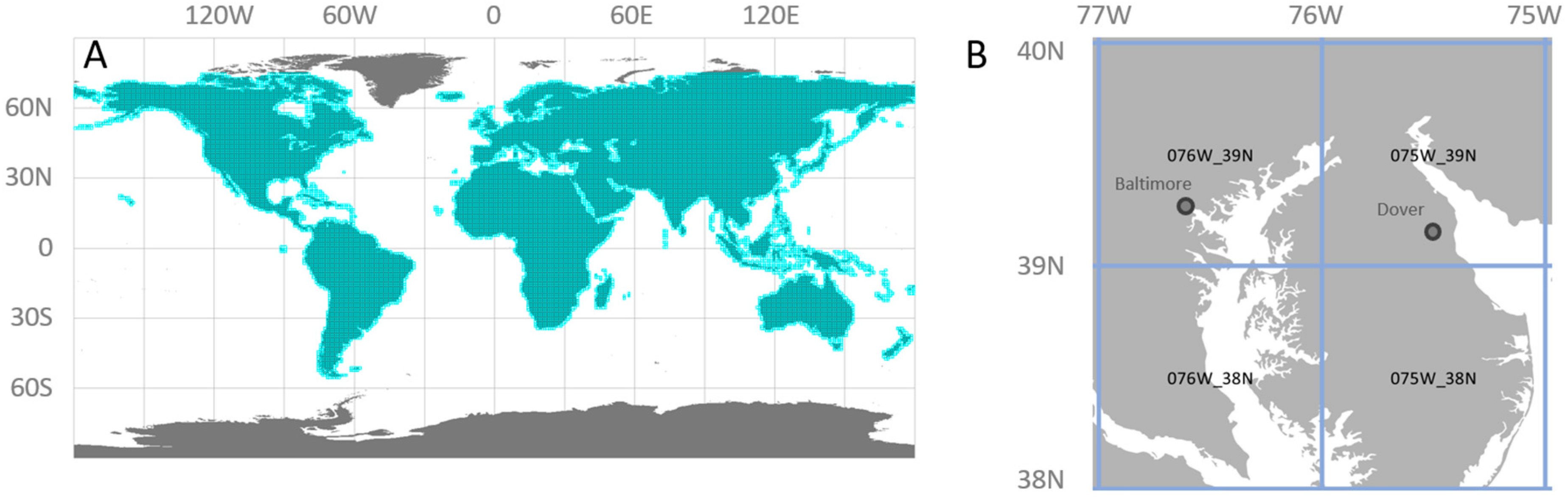
3.1. Global Tile System

The GLAD ARD tile system was developed to simplify global data handling. The geographic coordinates using the World Geodetic System (WGS84) were selected as the most universal way of sharing global data. The coordinate system is defined by EPSG Geodetic Parameter Dataset as EPSG:4326 (https://spatialreference.org/ref/epsg/wgs-84/), or using PROJ standard (http://proj.org) as +proj=longlat +ellps=WGS84 +datum=WGS84 +no_defs. The nearest neighbor resampling may be used to re-project the geographic data into the original Universal Transverse Mercator (UTM) Landsat pixel grid without distortion, assuming that the output UTM zone is the same as for the source Collection 1 Landsat imagery.

The spatial resolution of the ARD dataset is 0.00025 degree per pixel, which corresponds to 27.83 m per pixel on the Equator. The pixel size is a compromise between the need to preserve the original Landsat data pixel size (30 m/pixel) and to avoid using a repeating decimal number for pixel size (which may cause problems with georeference precision).

The ARD product is stored in 1 × 1 geographic degrees tiles. The tile format facilitates data handling and the parallelization of data processing. The exact 1 × 1 degree tile format, however, is not optimal for contextual analysis when neighboring pixels are located on different tiles. We implemented a partial solution to this issue by creating a tile system with a 2-pixel overlap. The actual ARD tile size is 4004 × 4004 pixels, an extent of 1.0005 by 1.0005 degrees. The 2-pixel buffer allows implementing contextual analyses using 3 × 3 and 5 × 5 kernels without the need to read data from multiple tiles at a time.

Tile names are derived from the tile center, and refer to the integer value of degrees. E.g., the name of a tile with center 17.5E and 52.5N is 017E_52N. The ARD product is only generated for tiles that include ice-free land area and where Landsat Tier 1 data exist (Figure 7). The tile names are used for folder structure only. The tile system can be downloaded from https://glad.umd.edu/ard/home in ESRI Shapefile format.

3.2. 16-Day Composite Data

Each data granule contains observations collected during a single 16-day interval. There are 23 intervals per year (see Table 5 for interval dates). Each interval has a unique numeric identification, starting from the first interval of the year 1980. This identification is used as a file name, while the tile name is used to identify data folders (Section 3.1). Equation (6) shows how to obtain the interval identification number for a selected year and season.

ID = (Year − 1980) × 23 + Interval

(6)

ID—interval identification number (file name), Year—selected year (1980 and later), Interval—selected annual 16-day interval (1–23).

The 16-day data for a tile are stored as 8-band, 16-bit unsigned, LZW-compressed GeoTIFF files. The list of image bands is provided in

Table 6. 16-day composite image layers.

Image Band	Image Data	Units, Data Format
1	Blue band	Normalized surface reflectance scaled to the range from 1 to 40,000, UInt16
2	Green band
3	Red band
4	NIR band
5	SWIR1 band
6	SWIR2 band
7	Normalized brightness temperature	K × 100, UInt16
8	Observation quality flag (QF)	QF code, UInt16

(see Table 1 for Landsat band abbreviations and wavelengths). The image band 8 consists of an observation quality flag (QF) that reflects the quality of observation used to create the composite. The QF (Table 3) is inherited from the Landsat image which is selected for the 16-day composite. QF values 1, 2 and 15 indicate clear-sky observations. QF values 11–14 and 16–17 are considered clear-sky data with an indication of cloud/shadow proximity. QF values 5 and 6 indicate seasonal data quality issues (topographic shadows and snow cover). These observations may be removed from data processing if the number of clear-sky observations is sufficient. QF values 3, 4, and 7–10 are considered contaminated by clouds and shadows and are usually excluded from data processing.

4. Multi-Temporal Metrics

Despite the global radiometric consistency of the 16-day GLAD ARD product, direct application of this dataset as input to a land cover characterization model is hampered by the irregular frequency of clear-sky observation. The availability of clear-sky observations is a function of the Landsat orbital constellation, data acquisition strategy, and cloud cover. As a result, annual 16-day time-series for the same area may have dramatically different numbers of clear-sky observations between seasons and years [19]. While 16-day time-series data contain sufficient information to identify land cover types and land cover dynamics (Figure 8), the inconsistency of observation frequency may not allow calibration of a regional mapping model using solely ARD as source data.

The multi-temporal metrics method is a time-series data transformation that improves spatial and temporal consistency, simplifies phenological analysis, and facilitates land cover mapping and change detection at large geographic extents. The metrics approach helps to overcome the inconsistency of clear-sky data availability that is typical for sensors with low observation frequency, such as Landsat. The metrics method was developed in the mid-1980s to extract phenological features from the AVHRR-based NDVI time-series [35,36]. At the same time, the idea of using vegetation index time-series to extract spectral reflectance corresponding to a certain phenological stage was proposed by Holben [37]. Later, both approaches were merged by researchers from the Laboratory for Global Remote Sensing Studies at the University of Maryland [38]. In their work, metrics were calculated by extracting spectral information for specific phenological stages defined by the NDVI annual dynamics. The multi-temporal metrics were widely used for forest monitoring at continental and global scales using MODIS [39] and Landsat data [6,19,20,40].

ARD-based multi-temporal metrics represent a set of statistics extracted from a 16-day observation time-series. The metric types and statistical algorithms may vary depending on the mapping objective. Here, we present algorithms for the two most common objectives: annual land cover mapping and detection of land cover changes between two consecutive years. To benefit these objectives, we use GLAD ARD data to create two independent sets of multi-temporal metrics: annual phenological metrics and annual change detection metrics. The metric processing tools and supervised classification tools that allow metrics characterization are available at https://glad.umd.edu/ard/home.

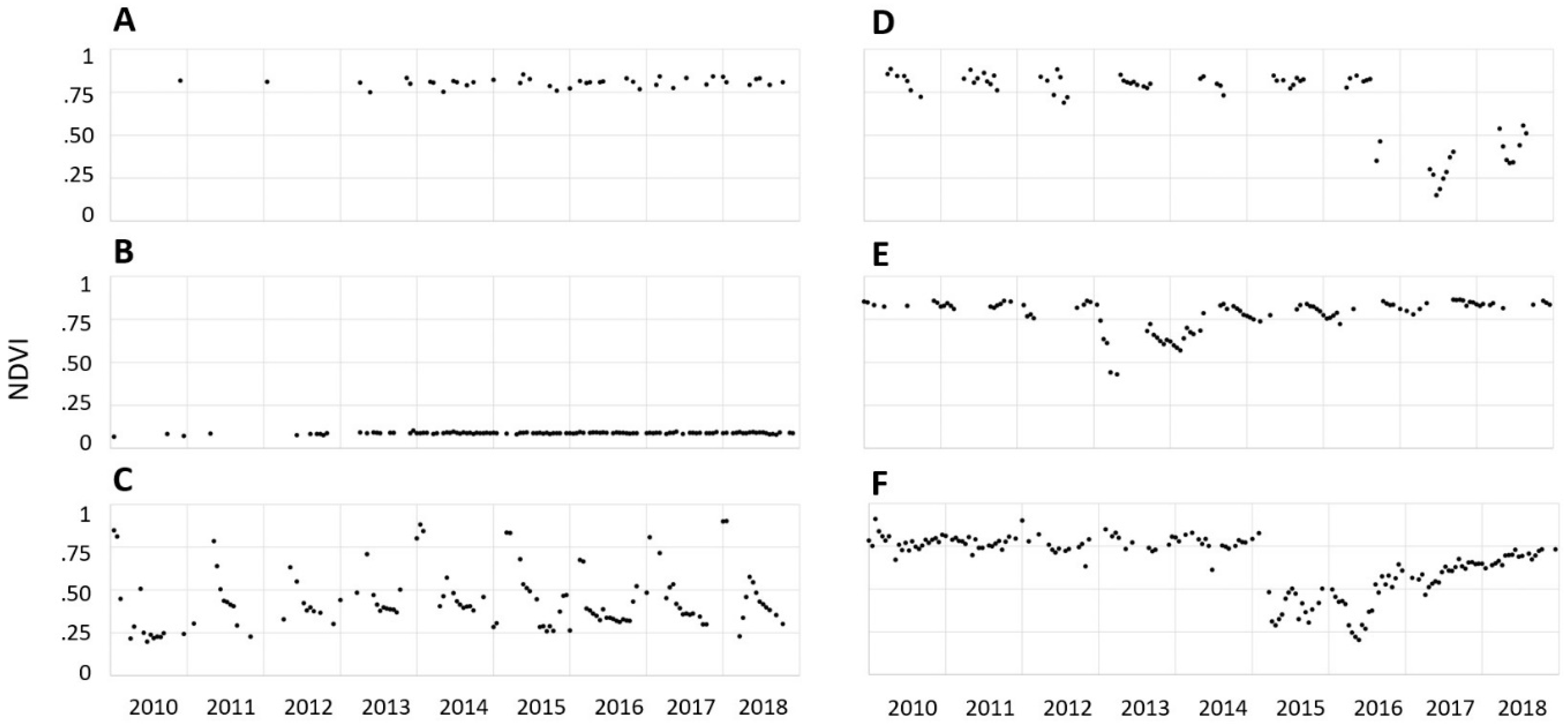
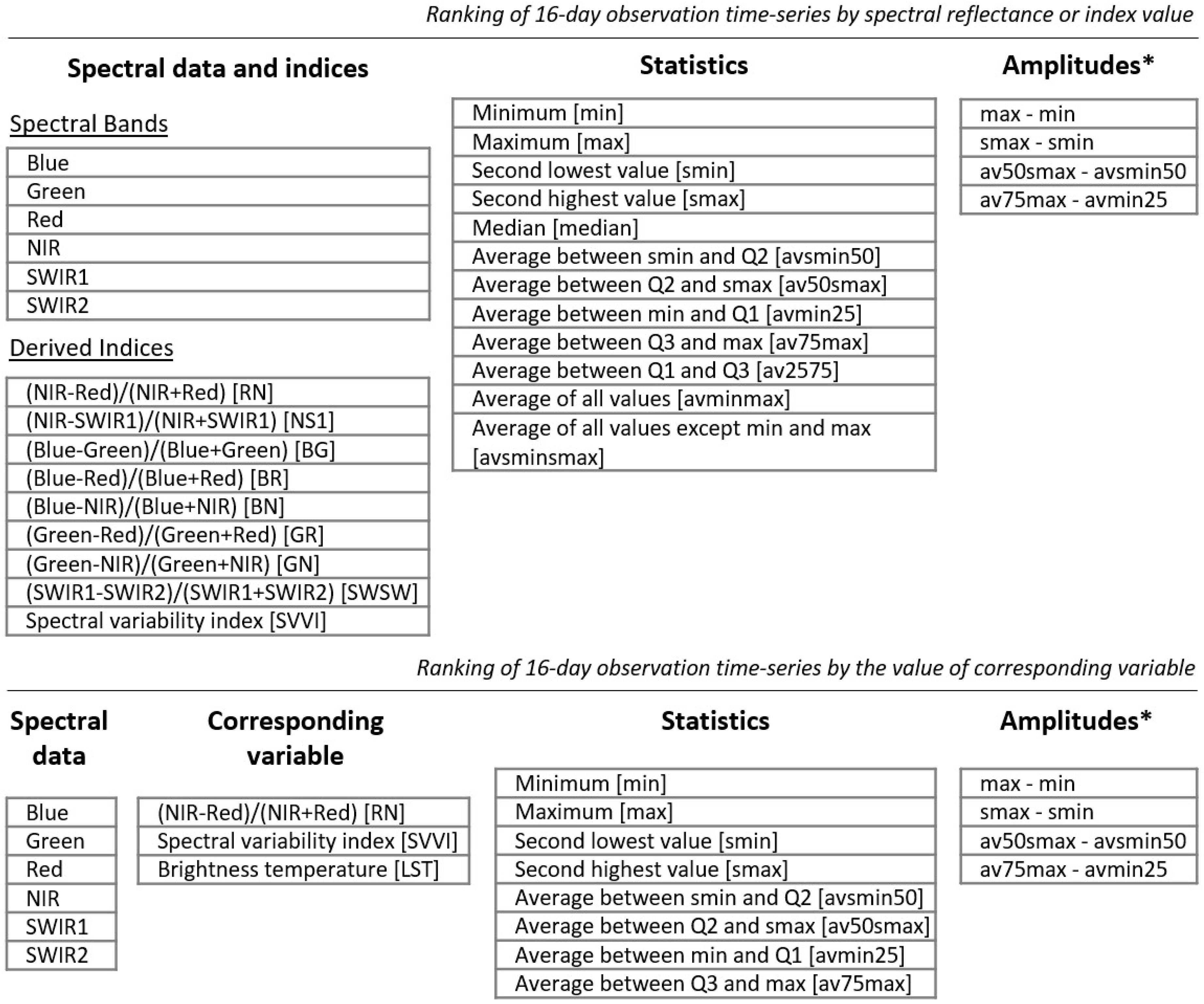
4.1. Annual Phenological Metrics

The annual phenological metrics serve as source data for land cover, land use, and vegetation structure mapping models. Metrics represent a set of statistics extracted from the normalized surface reflectance time-series within a corresponding calendar year (January 1–December 31). However, limited and inconsistent data availability in regions with a short snow-free season or frequent cloud cover may preclude consistent phenology characterization by annual observation time-series. To fill long gaps in observation time-series we use the data from the three previous years. Optionally, the gap-filling algorithm can be disabled to create metrics solely from data collected during the corresponding year. The process of phenological metrics processing includes two stages: (1) selecting clear-sky observations and filling gaps in the observation time-series; and (2) extracting reflectance distribution statistics from the time-series of selected observations.

First, we compile a gap-filled time-series of annual observations with the lowest atmospheric contamination (Figure 9). The per-pixel criterion for 16-day data selection is defined based on the distribution of QFs within the four years of data. If clear-sky land or water observations are present in the time-series data, only those are used for subsequent analysis. If no such observations are found, the software changes the observation quality threshold for data inclusion, first allowing observations with proximity to clouds and shadows, and then allowing all available observations. To create an annual gap-filled observation time-series for metric extraction, we first analyze the duration of the gaps between existing 16-day clear-sky observations of the corresponding year (Year i). If a gap exceeds two months (four 16-day intervals), we search for the clear-sky observations in the previous years within the gap date range, starting with Year i-1 and until the Year i-3. When clear-sky observations are found, they are added to the gap-filled time-series data, and the gap analysis is performed again until all gaps longer than two months are filled or no available data are found within the four-year interval.

After compilation of the annual gap-filled observation time-series, we compute selected normalized band ratios, or indices, for each selected observation using Equation (7). A spectral variability vegetation index (SVVI, [41]) is also calculated using the standard deviation of spectral reflectance values for each pixel (Equation (8)).

NR^AB = (ρ^A − ρ^B)/(ρ^A + ρ^B) × 10,000 + 10,000

(7)

NR^AB—Normalized ratio between bands A and B; ρ^A, ρ^B—normalized surface reflectance of bands A and B.

SVVI = σ (ρ^Blue, ρ^Green, ρ^Red, ρ^NIR, ρ^SWIR1, ρ^SWIR2) − σ(ρ^NIR, ρS^WIR1, ρ^SWIR2) + 10,000

(8)

SVVI—Spectral variability vegetation index; σ—standard deviation; ρ^Blue, etc.—normalized surface reflectance.

Multi-temporal metrics are generated from the time-series using two observation date ranking approaches (Figure 10). First, we rank all observations by each spectral band reflectance or index value individually. From obtained ranks, we select the highest/lowest, second to the highest/lowest, and median reflectance values. Also, we calculate averages for all observations between selected ranks (see Figure 10 for the list of average values). Second, we rank observation dates by corresponding values of (i) NDVI, (ii) SVVI, and (iii) brightness temperature. From these observation date ranks, we extract values corresponding to the highest/lowest, and second to highest/lowest ranks for each of the reflective bands, and calculate average reflectance values between selected ranks. In addition to spectral metrics, the software produces a set of auxiliary layers including the number of clear-sky 16-day composites, observation quality, and water presence per pixel.

The metrics are stored as single-band 16-bit unsigned GeoTIFF files using the same tile system as the ARD (see Section 3.1). The metrics set for each tile is stored in a separate folder. The metric naming convention is the following (see Figure 10 for bands, indices and statistics names):

YYYY_B_S_C.tif

YYYY—Corresponding year.

B—Spectral band or index.

S—Statistic extracted from the observation time-series.

C—Corresponding band or index used for observation ranking (only for metrics extracted from ranks defined by a corresponding value).

Example:

2018_blue_max_RN.tif—The metric represents the value of the normalized surface reflectance of the Landsat blue band for the 16-day interval that has the highest red/NIR normalized ratio (also known as NDVI) value during the year 2018.

Not all of the metrics are recorded to disk. Specifically, the amplitude metrics are calculated in memory during the classification procedure. To include spatial context to image classification, the focal mean for each of the metric using 3 × 3 kernel is calculated during the classification routine.

The large number of multi-temporal metrics (816 metrics in the phenological metrics set described above) is warranted by the large variety of land cover classes that may be mapped using these data. Different metrics and their combination highlight specific features of the surface reflectance and land surface phenology that are required for mapping different land cover types. The simple interquartile reflectance average (average of all values between 1st and 3rd quartiles, each spectral band ranked independently by its value) may serve as a generic clear-sky image composite for a specific year (Figure 11A). If the observations are ranked by the corresponding NDVI value, and the average is calculated from the top ranks, the composite will represent surface reflectance during the peak of the growing season (Figure 11B). Metrics extracted from the NDVI and brightness temperature ranks are required for agriculture mapping [23,42,43]. The spectral reflectance amplitudes highlight the land surface phenology and simplify identification of evergreen trees, permanent water features, and crop rotation characterization (Figure 11C). Using normalized ratios and their phenology facilitates mapping of different land cover types and simplifies visual assessment (Figure 11D).

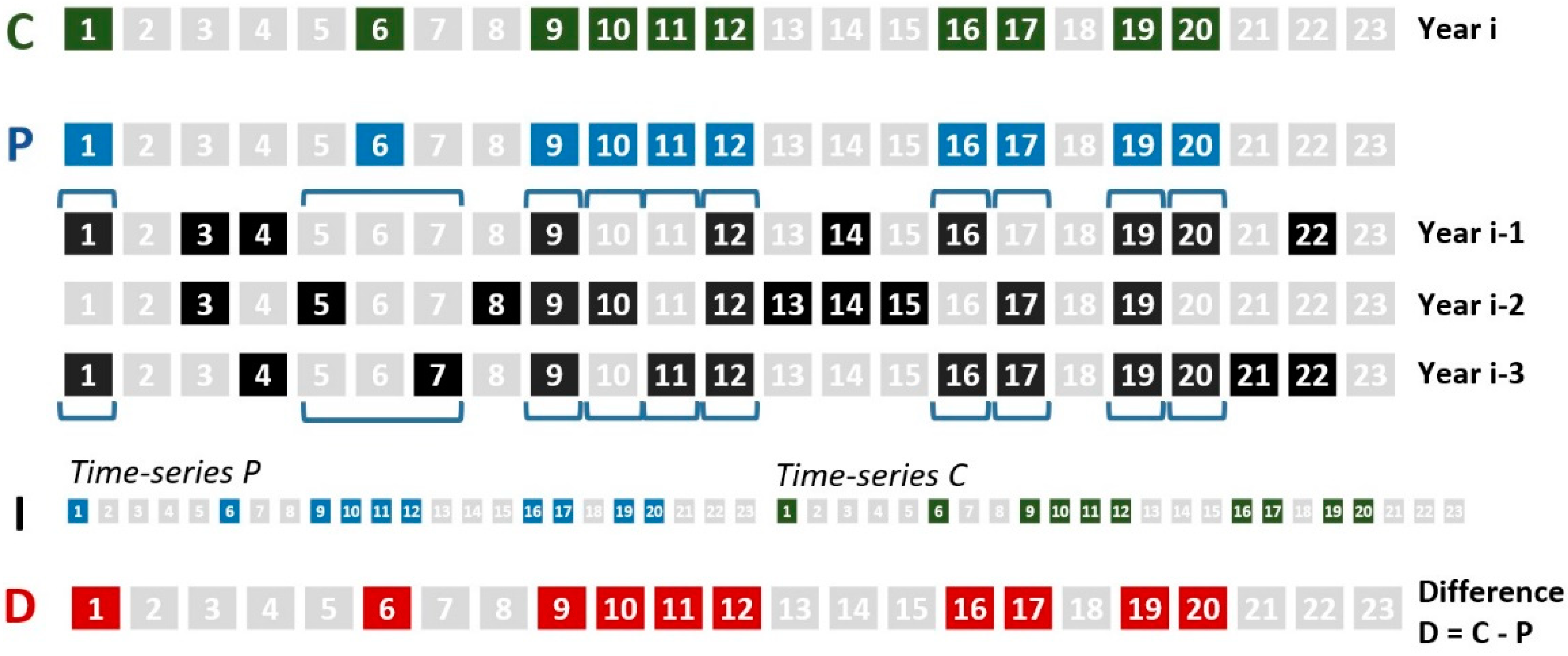
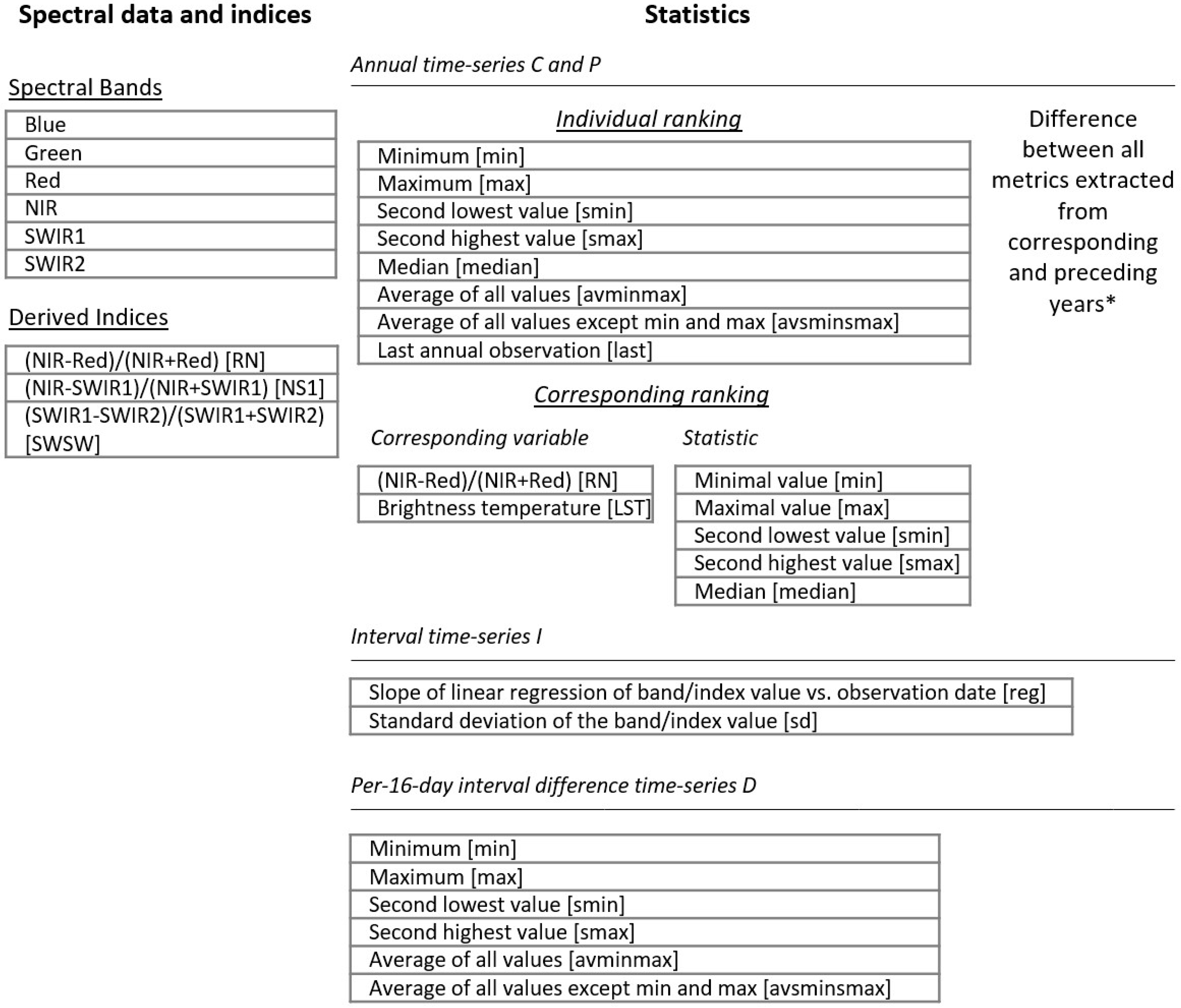
4.2. Annual Change Detection Metrics

The annual change detection metrics are designed to facilitate land cover change mapping between the corresponding and previous years while reducing false change detections due to reflectance fluctuations and inconsistent clear-sky observations availability. Change detection metrics describes the surface reflectance within the corresponding and preceding years, spectral reflectance differences between these years, and surface reflectance trend within the time-series. The process of change detection metrics construction includes three stages: (1) selecting clear-sky observations; (2) constructing data time-series, and (3) extracting reflectance and reflectance change distribution statistics from the time-series.

To build a set of change detection metrics, we utilize four years of data (one corresponding and three preceding), and select observations with the best available quality. The metric set can be generated with less than four years of data, but at least two consecutive years of data are required. Only observations with the lowest atmospheric contamination are used for metrics extraction. The per-pixel criterion for 16-day data selection is defined automatically based on the distribution of observation quality flags within the four years of data, similar to the phenological metrics algorithm. All other observations are discarded from further processing.

To facilitate extraction of the change detection data, we construct four different data time-series (time-series C, P, I, and D, see Figure 12). Time-series C comprised from the clear-sky observations of the corresponding year (Year i). To create a historical baseline for change detection (time-series P), we collect an average reflectance from the three preceding years (Year i-1–Year i-3) only for those 16-day intervals that have clear-sky observations in the time-series C. If no observations are found for a certain 16-day interval in historic data, we use clear-sky data from the closest observation before/after the missing 16-day composite interval. For each observation of time-series C and P, in addition to normalized reflectance, we calculate normalized ratios from selected bands (Equation (7)). Time-series P and C are further aggregated into a single, 46-interval, time-series to calculate trend analysis metrics (time-series I). Finally, the per-16-day interval difference for all spectral band and index values between time-series P and C comprise the time-series D.

To extract statistics, we use three different approaches (Figure 13):

• For the time-series C and P, we extract two independent sets of metrics that reflect annual phenology. Observations in each time-series are ranked by (a) spectral band or index value, and (b) corresponding NDVI and brightness temperature values. Similar to phenological metrics, we record selected ranks and average between ranks for each spectral variable.
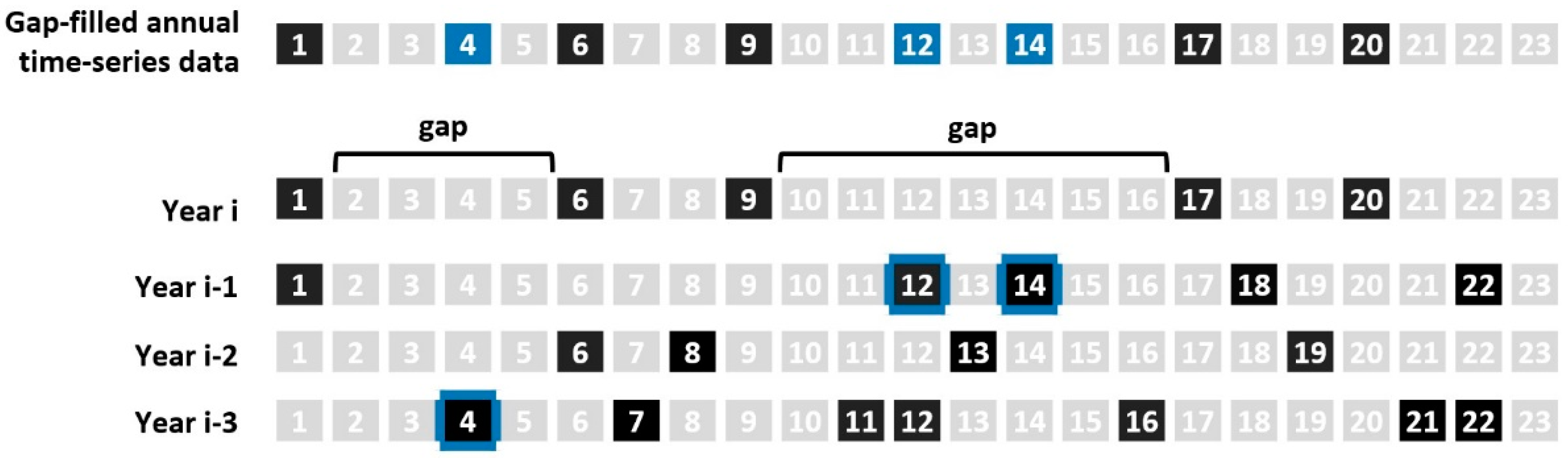
• The time-series I is used to analyze unidirectional trend of spectral reflectance within a two-years interval. We use least squares method to fit linear regression model that predicts spectral reflectance or index value from the observation date (date range is from 1 to 46) for clear-sky observations. We record the slope of linear regression as a metric value. In addition, we calculate and record standard deviation of spectral variable within the time-series I.
• The time-series D consists of per-16-day interval spectral reflectance or index differences. We rank difference values, and extract a set of statistics (selected ranks and averages) from these ranking.

Similar to the phenological metrics, each metric is stored as a single-band 16-bit unsigned GeoTIFF file, and metrics are organized in folders named with corresponding tile names. The generic naming convention is the following:

YYYY_B_T_S_C.tif

Where:

YYYY—corresponding year.

B—Spectral band or index.

T—Time-series from which the statistics were extracted. Index [c] represents the corresponding year (time-series C), [p] stands for the preceding year (time-series P) and [dif] stands for a time-series of per-16-day interval differences (time-series D). Slope of linear regression and standard deviation metrics, which are calculated from the entire time-series, do not have this name section.

S—Extracted statistic.

C—Corresponding band or index used for ranking (only for metrics extracted from ranks defined by a corresponding value).

Example:

2018_blue_c_max_RN.tif—The metric represents the value of the normalized surface reflectance of the Landsat blue band for the 16-day interval that has the highest red/NIR normalized ratio (also known as NDVI) value during the year 2018.

The high variability of metrics allows using the generic change detection metric set for the wide spectrum of land cover monitoring applications. Annual metrics for the corresponding and preceding years (Figure 14A,B) are compared by calculating differences during change detection model parametrization to indicate land cover change. The inter-annual spectral reflectance difference can be visualized by combining the same statistics extracted from different years (Figure 14C). Metrics that represent the slope of linear regression, and statistics extracted from per-16-day differences (Figure 14D) provide important information on land cover change [19,20,29].

Annual change detection metrics serve the operational update of the global forest cover change product that is developed by the GLAD team for Global Forest Watch initiative (www.globalforestwatch.org). The data users should be aware that while using four years of data to create a change detection metrics set improves the classification quality, the metric set is sensitive to changes that happened not only between the corresponding and preceding years, but also between the corresponding year and the years i-2 and i-3. The “last annual observation” metric may be used to exclude changes that happened earlier. Alternatively, a change detection algorithm can be applied annually to eliminate redundant change detections.

5. Known Issues and Limitations

The GLAD team is constantly updating the ARD product to ensure data completeness and quality. Here, we list known issues that users should consider when using the product. Some of these issues will be addressed in future revisions of the GLAD ARD.

• The current version of the GLAD ARD product is not suitable for real-time land cover monitoring. The ARD product rely on Tier 1 data which currently features up to 26 days processing delay by USGS (https://www.usgs.gov/land-resources/nli/landsat/landsat-collection-1). A 16-day interval data are processed only after all daily data are available as Tier 1. Thus, the ARD update usually features a 1-month delay.
• Landsat 5 images for 2001–2002 were filtered for possible sensor artifacts during ARD processing. However, after examining images recently processed to Collection 1 standard we suggested that some of these artifacts were removed by the data provider. A re-processing of the year 2001 and 2002 ARD will be scheduled to include corrected L5 data.
• Images crossing the 180° meridian were not processed due to technical difficulties. This issue was not addressed yet due to low demand for the data in these regions. The images will be processed and the corresponding 16-day composites will be updated later.
• Due to low sun azimuth and similarity between snow cover and clouds during winter season in temperate and boreal climates, the GLAD Landsat ARD algorithm is not suitable for winter time image processing above 30N and below 45S Latitude. We are not processing images during times affected by seasonal snow cover so the resulting 16-day intervals have no data. Some of the images (and resulting 16-day composites) may still include snow-covered observations. We suggest further filtering such observations using the “snow/ice” observation quality flag or by removing certain 16-day intervals from data processing.
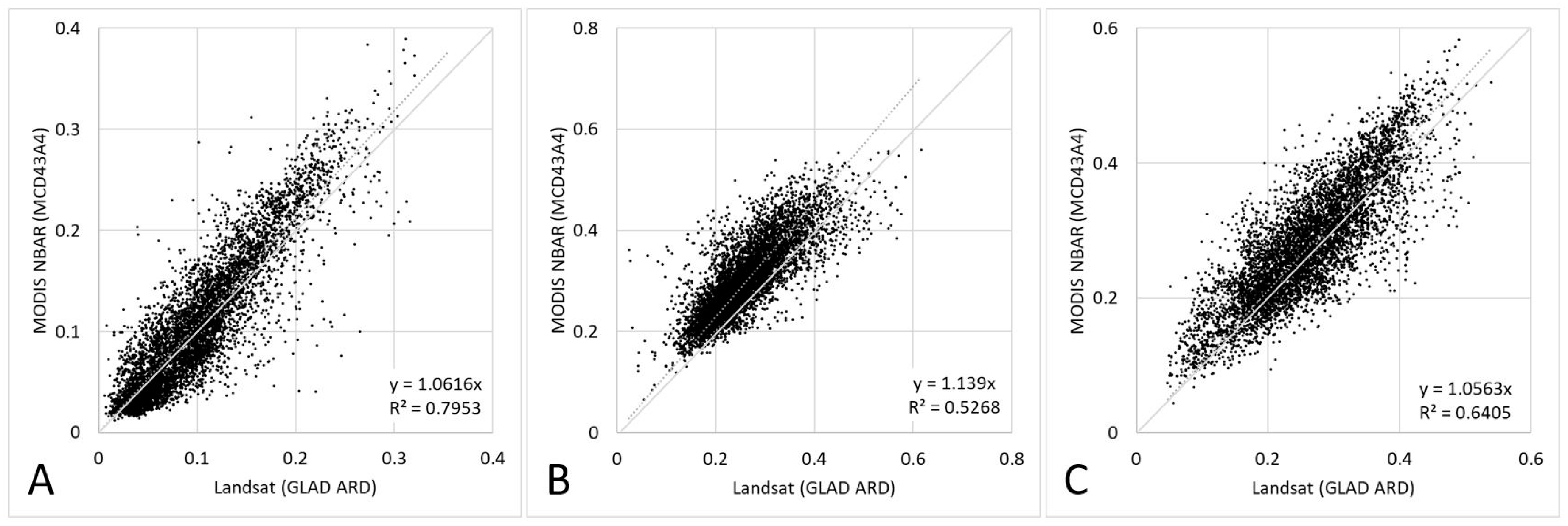
• The surface reflectance normalization is not equal to a physically-based atmospheric and surface anisotropy correction. While the comparison of ARD data with MODIS-based surface reflectance and successful ARD applications for global land cover mapping suggest that the product has sufficient quality for intended use, the ARD data may not be suitable for precise analysis of land surface reflectance.
• Users should be aware that the image normalization method is not designed to deal with specular reflectance and thus introduces bias over the water surfaces. We do not recommend using the ARD product for water quality assessment or any other hydrology applications beyond surface water extent mapping.

References

1. Woodcock, C.E.; Allen, R.; Anderson, M.; Belward, A.; Bindschadler, R.; Cohen, W.; Gao, F.; Goward, S.N.; Helder, D.; Helmer, E.; et al. Free Access to Landsat Imagery. Science 2008, 320, 1011a. [Google Scholar] [CrossRef] [PubMed]
2. USGS EROS. Landsat Collection 1 Level 1 Product Definition; USGS: Sioux Falls, SD, USA, 2017. [Google Scholar]
3. Wulder, M.A.; Masek, J.G.; Cohen, W.B.; Loveland, T.R.; Woodcock, C.E. Opening the archive: How free data has enabled the science and monitoring promise of Landsat. Remote. Sens. Environ. 2012, 122, 2–10. [Google Scholar] [CrossRef]
4. Wulder, M.A.; White, J.C.; Goward, S.N.; Masek, J.G.; Irons, J.R.; Herold, M.; Cohen, W.B.; Loveland, T.R.; Woodcock, C.E. Landsat continuity: Issues and opportunities for land cover monitoring. Remote. Sens. Environ. 2008, 112, 955–969. [Google Scholar] [CrossRef]
5. Hansen, M.C.; Loveland, T.R. A review of large area monitoring of land cover change using Landsat data. Remote. Sens. Environ. 2012, 122, 66–74. [Google Scholar] [CrossRef]
6. Hansen, M.C.; Potapov, P.V.; Moore, R.; Hancher, M.; Turubanova, S.A.; Tyukavina, A.; Thau, D.; Stehman, S.V.; Goetz, S.J.; Loveland, T.R.; et al. High-resolution global maps of 21st-century forest cover change. Science 2013, 342, 850–853. [Google Scholar] [CrossRef] [PubMed] [Green Version]
7. Pekel, J.-F.; Cottam, A.; Gorelick, N.; Belward, A.S. High-resolution mapping of global surface water and its long-term changes. Nature 2016, 540, 418–422. [Google Scholar] [CrossRef]
8. Gong, P.; Li, X.; Wang, J.; Bai, Y.; Chen, B.; Hu, T.; Liu, X.; Xu, B.; Yang, J.; Zhang, W.; et al. Annual maps of global artificial impervious area (GAIA) between 1985 and 2018. Remote. Sens. Environ. 2020, 236, 111510. [Google Scholar] [CrossRef]
9. Ying, Q.; Hansen, M.C.; Potapov, P.V.; Tyukavina, A.; Wang, L.; Stehman, S.V.; Moore, R.; Hancher, M. Global bare ground gain from 2000 to 2012 using Landsat imagery. Remote. Sens. Environ. 2017, 194, 161–176. [Google Scholar] [CrossRef] [Green Version]
10. DeFries, R.S.; Townshend, J.R.G. NDVI-derived land cover classifications at a global scale. Int. J. Remote. Sens. 1994, 15, 3567–3586. [Google Scholar] [CrossRef]
11. Loveland, T.R.; Belward, A.S. The IGBP-DIS global 1km land cover data set, DISCover: First results. Int. J. Remote. Sens. 1997, 18, 3289–3295. [Google Scholar] [CrossRef]
12. Hansen, M.C.; DeFries, R.S.; Townshend, J.R.G.; Carroll, M.; Dimiceli, C.; Sohlberg, R.A. Global Percent Tree Cover at a Spatial Resolution of 500 Meters: First Results of the MODIS Vegetation Continuous Fields Algorithm. Earth Interact. 2003, 7, 1–15. [Google Scholar] [CrossRef] [Green Version]
13. Justice, C.; Townshend, J.; Vermote, E.; Masuoka, E.; Wolfe, R.; Saleous, N.; Roy, D.; Morisette, J. An overview of MODIS Land data processing and product status. Remote. Sens. Environ. 2002, 83, 3–15. [Google Scholar] [CrossRef]
14. Price, R.D.; King, M.D.; Dalton, J.T.; Pedelty, K.S.; Ardanuy, P.E.; Hobish, M.K. Earth science data for all: EOS and the EOS data and information system. Photogramm. Eng. Remote Sens. 1994, 60, 277–285. [Google Scholar]
15. Roy, D.P.; Ju, J.; Kline, K.; Scaramuzza, P.L.; Kovalskyy, V.; Hansen, M.; Loveland, T.R.; Vermote, E.; Zhang, C. Web-enabled Landsat Data (WELD): Landsat ETM+ composited mosaics of the conterminous United States. Remote Sens. Environ. 2010, 114, 35–49. [Google Scholar] [CrossRef]
16. Dwyer, J.L.; Roy, D.P.; Sauer, B.; Jenkerson, C.B.; Zhang, H.K.; Lymburner, L. Analysis Ready Data: Enabling Analysis of the Landsat Archive. Remote Sens. 2018, 10, 1363. [Google Scholar]
17. Frantz, D. FORCE—Landsat + Sentinel-2 Analysis Ready Data and Beyond. Remote Sens. 2019, 11, 1124. [Google Scholar] [CrossRef] [Green Version]
18. Hansen, M.C.; Roy, D.P.; Lindquist, E.; Adusei, B.; Justice, C.O.; Altstatt, A. A method for integrating MODIS and Landsat data for systematic monitoring of forest cover and change in the Congo Basin. Remote. Sens. Environ. 2008, 112, 2495–2513. [Google Scholar] [CrossRef]
19. Potapov, P.; Tyukavina, A.; Turubanova, S.; Talero, Y.; Hernandez-Serna, A.; Hansen, M.; Saah, D.; Tenneson, K.; Poortinga, A.; Aekakkararungroj, A.; et al. Annual continuous fields of woody vegetation structure in the Lower Mekong region from 2000–2017 Landsat time-series. Remote. Sens. Environ. 2019, 232, 111278. [Google Scholar] [CrossRef]
20. Potapov, P.V.; Turubanova, S.A.; Hansen, M.C.; Adusei, B.; Broich, M.; Altstatt, A.; Mane, L.; Justice, C.O. Quantifying forest cover loss in Democratic Republic of the Congo, 2000–2010, with Landsat ETM+ data. Remote Sens. Environ. 2012, 122, 106–116. [Google Scholar] [CrossRef]
21. Pickens, A.H.; Hansen, M.; Hancher, M.; Potapov, P. Monitoring the dynamics of global surface water 1999–2017. In Proceedings of the AGU Fall Meeting, Washington, DC, USA, 9–14 December 2018. [Google Scholar]
22. Chavez, P.S. An improved dark-object subtraction technique for atmospheric scattering correction of multispectral data. Remote. Sens. Environ. 1988, 24, 459–479. [Google Scholar] [CrossRef]
23. Song, X.-P.; Potapov, P.V.; Krylov, A.; King, L.; Di Bella, C.M.; Hudson, A.; Khan, A.; Adusei, B.; Stehman, S.V.; Hansen, M.C. National-scale soybean mapping and area estimation in the United States using medium resolution satellite imagery and field survey. Remote. Sens. Environ. 2017, 190, 383–395. [Google Scholar] [CrossRef]
24. Chander, G.; Markham, B.L.; Helder, D.L. Summary of current radiometric calibration coefficients for Landsat MSS, TM, ETM+, and EO-1 ALI sensors. Remote Sens. Environ. 2009, 113, 893–903. [Google Scholar] [CrossRef]
25. Foga, S.; Scaramuzza, P.L.; Guo, S.; Zhu, Z.; Dilley, R.D.; Beckmann, T.; Schmidt, G.L.; Dwyer, J.L.; Hughes, M.J.; Laue, B. Cloud detection algorithm comparison and validation for operational Landsat data products. Remote. Sens. Environ. 2017, 194, 379–390. [Google Scholar] [CrossRef] [Green Version]
26. Zhu, Z.; Wang, S.; Woodcock, C.E. Improvement and expansion of the Fmask algorithm: cloud, cloud shadow, and snow detection for Landsats 4–7, 8, and Sentinel 2 images. Remote. Sens. Environ. 2015, 159, 269–277. [Google Scholar] [CrossRef]
27. Department of the Interior U.S. Geological Survey. Landsat 8 Data Users Handbook (LSDS-1574 Version 5.0); USGS: Sioux Falls, SD, USA, 2019.
28. Breiman, L.; Friedman, J.; Stone, C.J.; Olshen, R.A. Classification and Regression Trees; Taylor & Francis Group (CRC Press): Abingdon, UK, 1984. [Google Scholar]
29. Potapov, P.V.; Turubanova, S.A.; Tyukavina, A.; Krylov, A.M.; McCarty, J.L.; Radeloff, V.C.; Hansen, M.C. Eastern Europe’s forest cover dynamics from 1985 to 2012 quantified from the full Landsat archive. Remote Sens. Environ. 2015, 159, 28–43. [Google Scholar] [CrossRef]
30. Masek, J.; Vermote, E.; Saleous, N.; Wolfe, R.; Hall, F.; Huemmrich, K.; Gao, F.; Kutler, J.; Lim, T.-K. A Landsat Surface Reflectance Dataset for North America, 1990–2000. IEEE Geosci. Remote. Sens. Lett. 2006, 3, 68–72. [Google Scholar] [CrossRef]
31. Schaaf, C.B.; Gao, F.; Strahler, A.H.; Lucht, W.; Li, X.; Tsang, T.; Strugnell, N.C.; Zhang, X.; Jin, Y.; Muller, J.-P.; et al. First operational BRDF, albedo nadir reflectance products from MODIS. Remote. Sens. Environ. 2002, 83, 135–148. [Google Scholar] [CrossRef] [Green Version]
32. Vermote, E.F.; El Saleous, N.Z.; O Justice, C. Atmospheric correction of MODIS data in the visible to middle infrared: first results. Remote. Sens. Environ. 2002, 83, 97–111. [Google Scholar] [CrossRef]
33. Carroll, M.; Townshend, J.; Hansen, M.; Dimiceli, C.; Sohlberg, R.; Wurster, K. MODIS vegetative cover conversion and vegetation continuous fields. In Remote Sensing and Digital Image Processing; Springer: New York, NY, USA, 2011; Volume 11. [Google Scholar]
34. Huete, A.; Justice, C.; Van Leeuwen, W. MODIS vegetation index (MOD13). Algorithm Theor. Basis Doc. 1999, 3, 213. [Google Scholar]
35. Malingreau, J.-P. Global vegetation dynamics: satellite observations over Asia. Int. J. Remote. Sens. 1986, 7, 1121–1146. [Google Scholar] [CrossRef]
36. Badhwar, G. Classification of corn and soybeans using multitemporal thematic mapper data. Remote. Sens. Environ. 1984, 16, 175–181. [Google Scholar] [CrossRef]
37. Holben, B.N. Characteristics of maximum-value composite images from temporal AVHRR data. Int. J. Remote. Sens. 1986, 7, 1417–1434. [Google Scholar] [CrossRef]
38. DeFries, R.; Hansen, M.; Townshend, J. Global discrimination of land cover types from metrics derived from AVHRR pathfinder data. Remote. Sens. Environ. 1995, 54, 209–222. [Google Scholar] [CrossRef]
39. Hansen, M.C.; Stehman, S.V.; Potapov, P.V. Quantification of global gross forest cover loss. Proc. Natl. Acad. Sci. 2010, 107, 8650–8655. [Google Scholar] [CrossRef] [Green Version]
40. Potapov, P.; Siddiqui, B.N.; Iqbal, Z.; Aziz, T.; Zzaman, B.; Islam, A.; Pickens, A.; Talero, Y.; Tyukavina, A.; Turubanova, S.; et al. Comprehensive monitoring of Bangladesh tree cover inside and outside of forests, 2000–2014. Environ. Res. Lett. 2017, 12, 104015. [Google Scholar] [CrossRef]
41. Coulter, L.L.; Stow, D.A.; Tsai, Y.H.; Ibanez, N.; Shih, H.C.; Kerr, A.; Benza, M.; Weeks, J.R.; Mensah, F. Classification and assessment of land cover and land use change in southern Ghana using dense stacks of Landsat 7 ETM+ imagery. Remote Sens. Environ. 2016, 184, 396–409. [Google Scholar] [CrossRef]
42. King, L.; Adusei, B.; Stehman, S.V.; Potapov, P.V.; Song, X.-P.; Krylov, A.; Di Bella, C.; Loveland, T.R.; Johnson, D.M.; Hansen, M.C. A multi-resolution approach to national-scale cultivated area estimation of soybean. Remote. Sens. Environ. 2017, 195, 13–29. [Google Scholar] [CrossRef]
43. Khan, A.; Hansen, M.C.; Potapov, P.V.; Adusei, B.; Pickens, A.; Krylov, A.; Stehman, S.V. Evaluating Landsat and RapidEye Data for Winter Wheat Mapping and Area Estimation in Punjab, Pakistan. Remote. Sens. 2018, 10, 489. [Google Scholar] [CrossRef] [Green Version]
Figure 1. (A) Number of snow-free days used to select images for the ARD processing by WRS path/row. (B) Number of processed images 1997–2019 by WRS path/row.
Remotesensing 12 00426 g001
Figure 2. Total number of processed images per year and per Landsat sensor from January 1997 to October 2019.
Remotesensing 12 00426 g002
Figure 3. Example of calibration of the surface reflectance normalization model for the red spectral band of Landsat scene LC82240652019296LGN00. Median reflectance bias (scaled unitless, ρ × 40,000) was calculated between Landsat TOA reflectance and MODIS surface reflectance within the mask of pseudo-invariant objects for each of the 10,000 meters intervals of distance from the ground track. A linear regression model was used to model reflectance bias as a function of distance from the ground track. The model coefficients and R2 presented on the image.
Remotesensing 12 00426 g003
Figure 4. Geographic variation of the surface reflectance normalization coefficients. (A)—Red band coefficient B (bias). (B)—NIR band coefficient G (gain). Surface reflectance value is scaled unitless, ρ × 40,000.
Remotesensing 12 00426 g004
Figure 5. Global SWIR-NIR-Red composites of (A) MODIS surface reflectance used as a normalization target and (B) Landsat annual average normalized surface reflectance for the year 2018. The average reflectance is calculated from all clear-sky observations with band reflectance value between the 25th and 75th percentile. Observations affected by seasonal snow cover are excluded.
Remotesensing 12 00426 g005
Figure 6. Comparison of MODIS NBAR surface reflectance (MCD43A4 Version 6) and Landsat GLAD ARD normalized surface reflectance products for randomly selected clear-sky land observations for June–August 2018 within the conterminous United States (N = 6,099). Spectral bands: (A)—red, (B)—NIR, (C)—SWIR (1.6 μm).
Remotesensing 12 00426 g006
Figure 7. GLAD ARD tile system. (A)—global extent of processed data (tiles shown in blue), 1997–2019; (B)—example of tile extents and names. The tile system can be downloaded from https://glad.umd.edu/ard/home in ESRI Shapefile format.
Remotesensing 12 00426 g007
Figure 8. Examples of NDVI temporal profiles extracted from the 2010–2018 GLAD ARD clear-sky land observation time-series. Land cover types: (A)—Evergreen humid tropical forest, Democratic Republic of the Congo (Longitude: 25.63254, Latitude: 0.42928); (B)—Desert, Niger (11.37659, 18.22881); (C)—Rainfed agriculture, Brazil (−46.00316, −11.71092). Land cover change dynamics: (D)—Boreal forest harvesting, Canada (−80.50295, 47.79808); (E)—Shifting cultivation, Myanmar (95.52212, 26.13662); (F)—Pine plantation management, USA (−88.61679, 32.29155).
Remotesensing 12 00426 g008
Figure 9. Schematic representation of the gap-filling algorithm for phenological metrics. Year i stands for the corresponding year, and Years i-1–i-3 for preceding years. Black squares are clear-sky observations and gray squares are 16-day intervals with no data. The blue squares in the gap-filled time-series are clear-sky observations filled from the Years i-1–i-3 (highlighted by blue outlines) within the data gaps exceeding 2 months (four 16-day intervals).
Remotesensing 12 00426 g009
Figure 10. Phenological metric types and naming convention (metric names shown in square brackets). The first set of metrics represents statistics calculated from 16-day observation time-series ranked by the spectral reflectance or index value. The ranking performed independently for each spectral band or index. The second set of metrics represents statistics calculated from 16-day observation time-series ranked by the value of corresponding variable (NDVI, SVVI, and brightness temperature). Q1, Q2, and Q3 stand for 1st, 2nd, and 3rd quartiles. * Amplitudes are calculated in memory during classification model application and are not written to the disk.
Remotesensing 12 00426 g010
Figure 11. Example of image composites of different 2018 annual phenological metrics for Mekong Delta, Vietnam. (A) SWIR1-NIR-Red Q1-Q3 interquartile average reflectance composite, observations for each band ranked individually by their reflectance value; (B) NIR-SWIR1-SWIR2 Q3-max average reflectance composite, observations ranked by the NDVI value; (C) SWIR1-NIR-Red reflectance amplitude (difference between annual minimum and maximum) composite; (D) Red/NIR (NDVI)—Green/Red—NIR/SWIR2 second-to-maximum normalized ratios values, observations ranked individually by each ratio value.
Remotesensing 12 00426 g011
Figure 12. Schematic representation of the time-series data compilation for the change detection metrics. Green and black squares represent 16-day intervals with clear-sky observations, gray squares—16-day intervals with no clear-sky observations. C stands for the corresponding year time-series (Year i); P for preceding year time-series (average of Years i-1, i-2, and i-3, selected observations highlighted in blue). Time-series I is compiled from time-series P and C. D stands for difference between 16-day observations of C and P time-series (intervals with difference values highlighted in red).
Remotesensing 12 00426 g012
Figure 13. Change detection metric types and naming convention (abbreviations used for file names shown in square brackets). Annual statistics are collected independently for the corresponding and preceding years. Interval statistics are collected from a time-series of both years (46 observations). Per-16-day interval difference statistics are collected from the time-series of per-interval difference values. * Differences between metrics are calculated during the change detection model application and not written to disk.
Remotesensing 12 00426 g013
Figure 14. Composites of selected 2018 annual change detection metrics for Northern Laos (centered at 101.5950, 20.5473). (A)—SWIR1-NIR-Red Q1-Q3 interquartile average band reflectance composite for previous year (compiled from 2015–2017 data); (B)—SWIR1-NIR-Red Q1-Q3 interquartile average band reflectance composite for the year 2018; (C)—Interquartile average SWIR1 band reflectance difference between corresponding and previous years (red: corresponding year; blue, green—previous year); (D)—Composite of metrics based on per-16-day difference (red: maximum SWIR2 band difference; green and blue: average NIR/SWIR2 normalized ratio difference).
Remotesensing 12 00426 g014