
Peat Drainage Ditch Mapping from Aerial Imagery Using a Convolutional Neural Network


1
UK Centre for Ecology and Hydrology, Environment Centre Wales, Deiniol Road, Bangor LL57 2UW, UK
2
UK Centre for Ecology and Hydrology, Bush Estate, Penicuik EH26 0QB, UK
*
Author to whom correspondence should be addressed.
Remote Sens. 2023, 15(2), 499; https://doi.org/10.3390/rs15020499
Submission received: 21 November 2022
/
Revised: 6 January 2023
/
Accepted: 9 January 2023
/
Published: 14 January 2023
Abstract
:This study trialled a convolutional neural net (CNN)-based approach to mapping peat ditches from aerial imagery. Peat ditches were dug in the last century to improve peat moorland for agriculture and forestry at the expense of habitat health and carbon sequestration. Both the quantitative assessment of drained areas and restoration efforts to re-wet peatlands through ditch blocking would benefit from an automated method of mapping, as current efforts involve time-consuming field and desk-based efforts. The availability of LiDAR is still limited in many parts of the UK and beyond; hence, there is a need for an optical data-based approach. We employed a U-net-based CNN to segment peat ditches from aerial imagery. An accuracy of 79% was achieved on a field-based validation dataset indicating ditches were correctly segmented most of the time. The algorithm, when applied to an 802 area of the Flow Country, an area of national significance for carbon storage, mapped a total of 27,905 drainage ditch features. The CNN-based approach has the potential to be scaled up nationally with further training and could streamline the mapping aspects of restoration efforts considerably.
1. Introduction
Peatlands represent the most carbon-dense terrestrial ecosystems on the planet but have been heavily impacted by drainage for agriculture and forestry, making them major contributors to global anthropogenic CO emissions [1,2]. Reducing carbon emissions from peatlands is therefore an essential component of meeting environmental targets such as the Paris Climate Agreement. The most effective method of reducing emissions in almost all cases is through the rewetting and restoration of peatlands [3,4]. In the UK, peatlands account for over 10% of the land surface area and, despite considerable anthropogenic modification through drainage, are the largest terrestrial carbon store and provide a wide range of ecosystem functions [5,6]. Extensive drainage of the UK’s lowland fen peatlands for agriculture began in the 17th century, whereas the drainage of the more extensive blanket bogs of the uplands largely took place during the twentieth century. The cutting of ditches in the uplands, primarily intended to support extensive livestock grazing, grouse rearing, and plantation forestry, has caused long-term harm to these critical ecosystems [7]. Because the majority of drainage occurred on an informal basis, prior to the advent of digital record-keeping and geographic information systems, information on the extent and location of ditches is often very limited, which presents problems for the identification, management and restoration of impacted ecosystems. Mapping the location and extent of ditching is therefore an important component of peatland restoration, both to quantify affected areas (e.g., for national greenhouse gas emissions reporting) and to more efficiently target intervention. Mapping across large areas is time consuming (prohibitively so for the >2 million hectares of upland bog in the UK) and potentially subjective by field and/or desk-based methods [6]; hence, an automated method is needed, particularly with a view to data provision at regional and national scales. Remote sensing data and image processing techniques have much potential in this area, but automated methods for peat ditch mapping have so far been limited. Given the extent of ditching in the UK and the current drive to restore peatlands, with a target of 250,000 ha of restored peatland by 2030 in Scotland alone, understanding the potential of these techniques is an increasing priority.
Intact peatlands represent an important long-term carbon store as the rates of decomposition are lower than the uptake of carbon dioxide via photosynthesis due to the waterlogged nature of intact peat. However, in practice, many peatlands are now considered net emitters of carbon dioxide as drainage has lowered water tables and increased the oxidation of previously waterlogged peat, with over 1.5 million hectares of peatlands across the UK estimated to have been drained [8]. Water table depth has been shown to be a primary driver of the rate of greenhouse gas (GHG) fluxes from managed peatland systems [3], suggesting that measures to reverse the anthropogenic drainage of peatland systems could significantly reduce GHG emissions from peat oxidation and even return peatland systems to a state where the net GHG emissions are negative (i.e., emission of carbon dioxide and methane is lower than carbon dioxide uptake). Whilst the primary impact of peatland drainage is that it exacerbates the loss of carbon from the land to atmosphere, drainage can also affect carbon losses via the fluvial pathways that occur largely in the forms of dissolved and particulate organic carbon (DOC and POC, respectively). Emission factors have been developed for these waterborne fluxes to account for ‘off site’ emissions of CO that result from oxidation of DOC and POC that occurs downstream within the aquatic system [9]. In order to quantify the potential impact of peatland rewetting on national net zero targets, the current national peatland condition needs to be known. At present, there is no national-scale methodology for mapping peatland drainage [10], which is a major knowledge gap in our understanding of the potential for peatlands to contribute towards UK net zero targets. As current estimates of the potential contribution to GHG removal from peatlands in the UK are between 0 and 4.6 Mt CO by 2050 [11], uncertainties could be much reduced if the area of peat drained is quantified at a national scale. Remote sensing-based methods have the potential to contribute to reducing these uncertainties by providing a map of drained areas.
Peat ditches are relatively small-scale topographical features, necessitating the use of fine spatial resolution imagery to map them over large areas. Elevation-based data (typically LiDAR) are most suitable and can be used to map the presence of and change in topographical features where time series data are available [6]. Currently, the most accurate methods for mapping peat ditches are a combination of field-based surveying and manual digitisation from fine spatial resolution satellite, aerial imagery, or LiDAR [12,13]. This approach is exemplified by Carless et al. [12], where manual GIS-based methods were employed to delineate peat ditches in Dartmoor National Park, using a combination of LiDAR and multispectral data to visualise the drains as part of a study mapping peat-degradation features. Some attempts have been made at partial or complete automation of drainage ditch mapping in other contexts. Both Cazorzi et al. [14] and Bailly et al. [15] employ semi-automated methods to map anothopogenic drainage networks in agrarian landscapes using LiDAR. Connolly and Holden [16] used GeoEye satellite data and a semi-manual methodology to map peat ditches in Northern Ireland using commercial software (Feature Analyst). Rapinel et al. [17] applied an expert-driven rule base to LiDAR data to extract drainage ditches in a wetland in northeastern France. Roelens et al. [18] used a supervised machine learning-based approach to map drainage ditches in a small area of semi-urban wetland from a combination of LiDAR geometric and radiometric features. At present, fine spatial-resolution elevation data such as LiDAR are still not available for many areas of the UK and beyond. Furthermore, where LiDAR-based elevation data do exist, the point density is insufficient to delineate peat ditches, which are typically sub-metre in scale. Historic aerial imagery is more common; hence, there is a need to develop a method using optical data.
As optical data do not offer a direct representation of peat ditch morphometry, an image feature representation of peat ditches is required, typically involving a combination of planar edge features and colour. Classical image processing techniques, which typically use a combination of moving window filters, edge detectors, and expert-based decisions lack the flexibility to generalise over large varied feature sets and are not suitable [19,20]. Supervised machine learning (ML) is a better candidate, given the potential complexity of the feature space that defines peat-drains from optical data. However, ML techniques that operate on single data points still require hard-coded feature sets to cover both the shape and colour of the ditches and ultimately lack a global representation of the objects of interest. Convolutional Neural Nets (CNNs) combine hierarchical feature generation and learning into one algorithm and have emerged in the last decade as the cutting-edge approach for computer vision labelling tasks [21,22,23,24,25]. CNNs rely on rectilinear patches to learn a pattern corresponding to particular classes [26,27]. Essentially, the network learns a hierarchical feature representation of the image patch(es) through a process of down- (max-pooling) and then up-convolution (up-sampling) [21]. A multitude of CNN architectures have been developed over the past decade or so, first to label entire images, and then later adapted to per-pixel classification (usually termed semantic segmentation), where the class probabilities within the patch over a certain threshold correspond to membership.
Given that peat ditches are defined by both their colour and planar-shape from RGB imagery, a CNN should be well suited to mapping them, for its ability to encapsulate spatial and spectral information at multiple scales. CNNs have already shown promising results when applied to aerial imagery in the contexts of mapping land-cover, vegetation types, species, and landscape features [20,23,28]. Given their ability to learn task-specific features and efficacy in other contexts, we trial a CNN-based approach to mapping peat-drainage ditches. To this end we utilise a U-Net-based model [21], a widely used semantic segmentation architecture that is well suited to planar-view data.
To test the efficacy of a CNN-based ditch mapping approach, we chose the Flow Country of Northern Scotland, a nationally significant peatland in terms of carbon storage and the largest blanket bog in Europe [29]. Based on its unique natural characteristics, the Flow Country was nominated in 2020 by the UK Government for UNESCO World Heritage Status. However, the region has been subject to very extensive drainage of both areas remaining under blanket bog vegetation and large areas of conifer plantation developed during the late 20th century, which both threaten the long-term stability of the ecosystem. Whilst peatland subsidence has been assessed in the area using satellite-based interferometric techniques [30], we are not aware of outputs pertaining to ditching extent other than manual field/desk-based assessments. These data are essential if this and other vulnerable peatland regions, both in the UK and globally, are to be effectively conserved.
2. Materials and Methods
2.1. Study Site
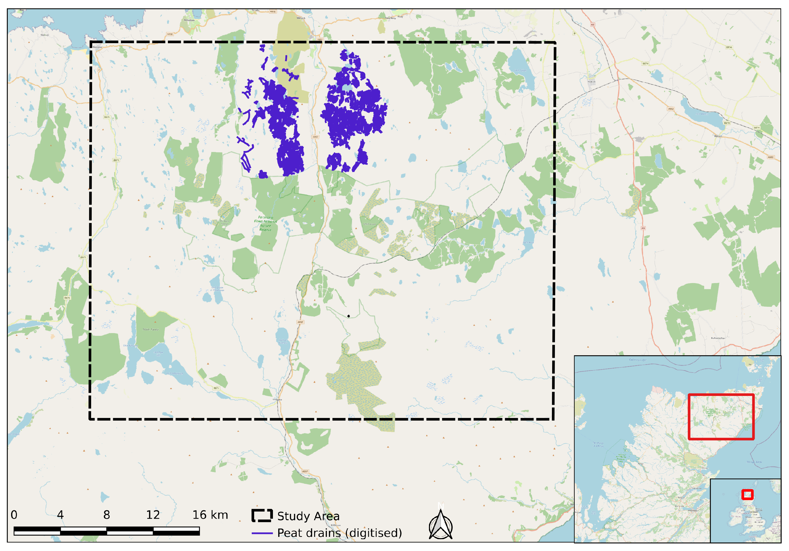
The subset of the Flow Country delimited for CNN-based mapping is displayed in Figure 1, with the manually mapped peat ditches in blue. The area of interest is centred on the settlements of Upper Bighouse and Dalhalvaig and is split by the A897 road from north to south. The area is known to be extensively ditched, with large areas of drained for afforestation in the 1980s and other areas of remaining blanket bog ditched with the intention of increasing grazing quality, primarily for deer. Intact peatland with little evidence of anthropogenic disturbance is also present. Ditching to the north of the study area has been manually mapped using a combination of aerial imagery and field-based validation (Figure 1) and made available for this investigation.
2.2. Aerial Imagery and Field Data
The aerial imagery was collected between 2011 and 2014 as part of the Next Perspectives consortium on behalf of the UK government. The imagery consists of RGB bands at a per-pixel X,Y resolution of 25 cm, a subset of which provides the backdrop in Figure 2.
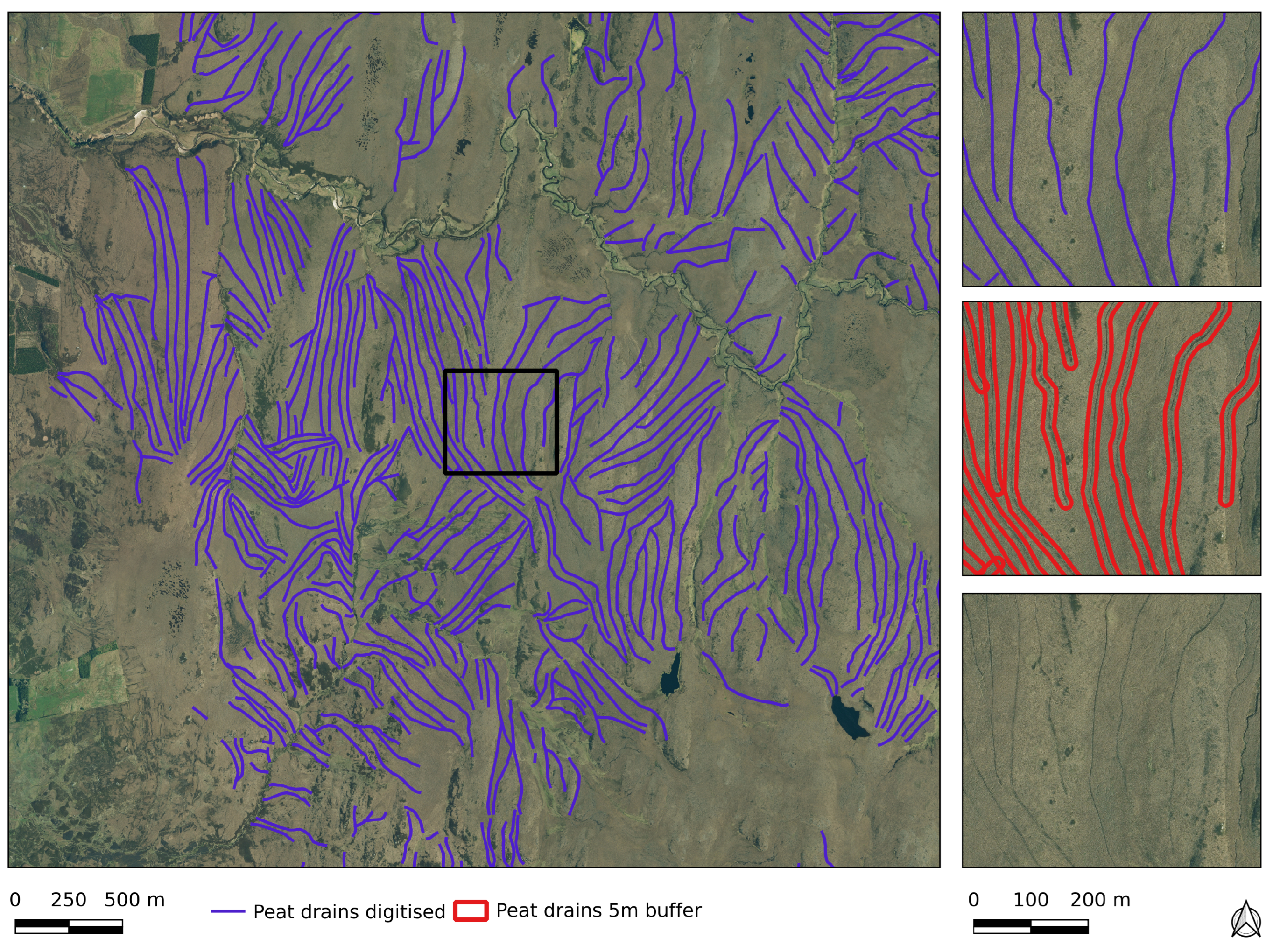
Peat ditches were mapped by NatureScot as part of the Peatland ACTION project (Figure 1) using a combination of aerial imagery and field-based validation, the output of which was a polyline GIS file (Figure 2). At this stage, the polylines had no representation of channel width and required a buffer to become a planar approximation of the peat ditch and banks. As the drainage ditch channel widths and accuracy of the field mapped polylines vary, a relatively wide buffer was required to ensure that each peat ditch channel was covered. Consequently the polylines were buffered by 5 m to produce a set of polygons in order to give each object a width and represent the pixel variation of each peat ditch. In this context, each drain ‘object’ consists of both the channel and vegetated banks. Polygons were then rasterised, producing a binary map of peat ditches at the pixel resolution of the underlying imagery. The expectation, therefore, is that the labelled output will approximate both banks and drainage channel.
2.3. Image Processing and CNNs
2.3.1. Pre-Processing and Training Augmentations
The binary training maps produced from the field data were subdivided into chips of 256 by 256 pixels, and only those containing the positive class pixels were retained. The data were then randomly split into training (60%), testing (20%), and validation (20%) sets for training and evaluation of the CNN algorithm’s performance. The training and testing sets were monitored in parallel to ensure that over-fitting did not occur, with the validation set used in the accuracy assessment. All pre- and post-processing was carried out using Geospatial-learn [31], itself principally reliant on the Scipy-stack, Scikit-learn, GDAL and Pytorch libraries [32,33,34,35].
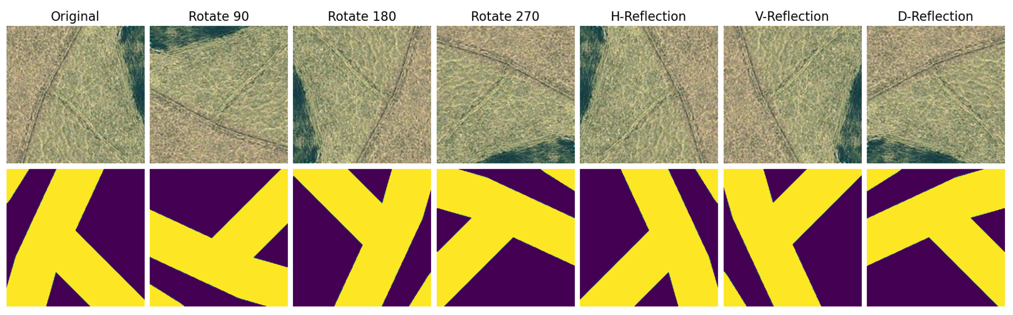
Data augmentation is widely used to expand limited training sets for CNNs and is utilised in this study. Augmentation involves the rotation, filtering, cropping, or warping of the existing training imagery to produce additional training examples. The augmentations were limited to non-destructive transformations as the planar view/perspective is not variable. Images and corresponding training masks were rotated/reflected through dihedral group permutations (Figure 3).
2.3.2. CNN Overview and Model Choice
As CNNs often require a considerable amount of training data to be provided from scratch, transfer learning is commonly used with limited training data, whereby a pre-trained network is fine tuned with a new set of training/classes. If the original pre-trained network has learned from a sufficiently large and varied image collection, it should act a surrogate for a generic image feature generator. This study employs the transfer learning approach and utilises the widely used Res-net encoder and U-net decoder architectures as implemented in Pytorch [35]. Res-net utilises skip connections to ensure the loss surface remains smooth/navigable, ensuring efficient training and accurate results despite a dense network structure [27].
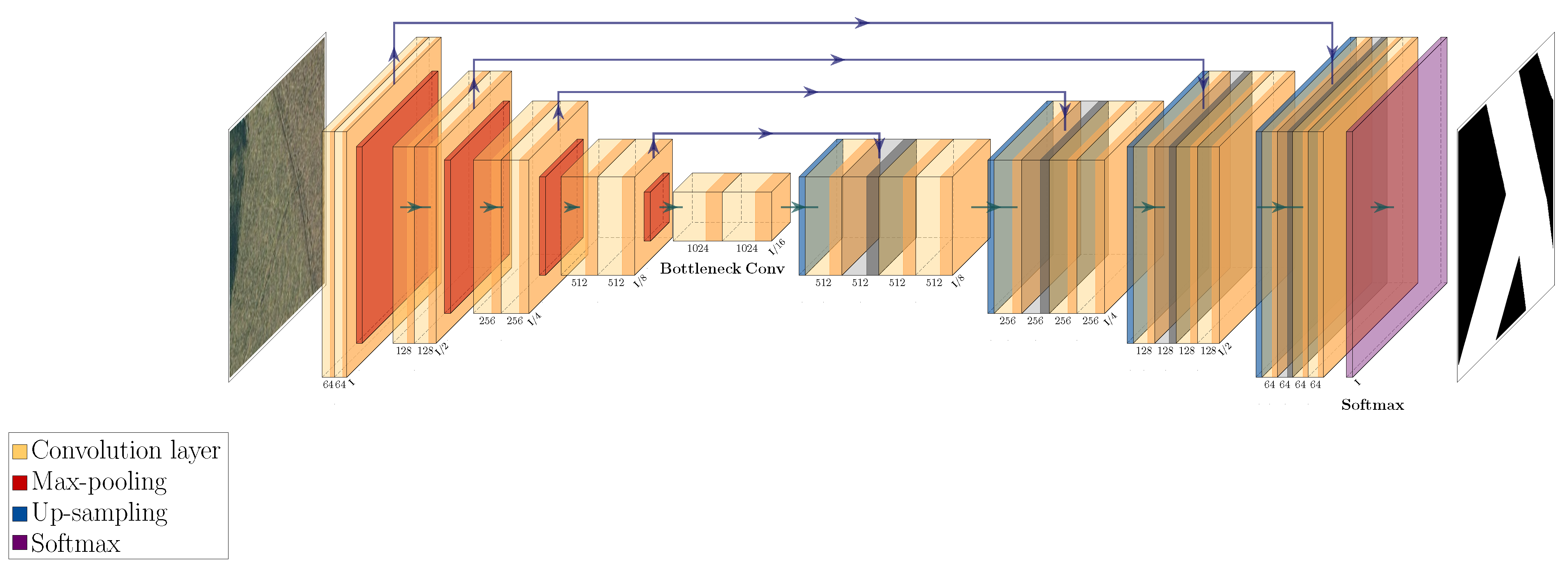
A schematic of the CNN used is displayed in Figure 4, where imagery is propagated through the network via a series of non-linear activation functions to produce a binary segmentation map.
The network connections are represented by the arrows linking the encoder and decoder segments. Each yellow panel in the schematic represents a convolutional layer, with the feature depth therein annotated at the foot of each, with the max-pooling/up-sampling fraction to the right of these. From left to right, an input image is ingested, and the encoder produces feature maps at each convolutional layer, of which the maximum response values are propagated to the next via a max-pooling operation (red panels). At each layer of the encoder, the max pooling operation extracts the maximum value within a sliding window in order to reduce the dimensions of the feature maps and thus the number of parameters the network has to learn. This process is analogous to changing the emphasis from the spatial aspects of the image, to the class identity with depth in the network. The reverse is then applied via up-convolutions (blue panels) to reconstruct from the deepest feature map, eventually resulting in a soft-max-based probability map (pink panel), from which a per-pixel mask is produced from a predefined threshold.
2.3.3. Accuracy Assessment
Segmentation accuracy was measured using the F score, which is the harmonic mean of precision and recall. Precision represents the percentage of all classified pixels that were classified correctly (true positives), the inverse of which is an error of commission. Recall represents the percentage of pixels correctly classified compared with the reference data, the inverse of which is an error of omission.
Where tp are true positives, fp are false positives, fn are false negatives.
3. Results
Accuracy
The model was trained for 30 epochs and achieved a training set accuracy of 0.9. When the model was tested on the validation data, an score of 0.79 was achieved (Table 1).
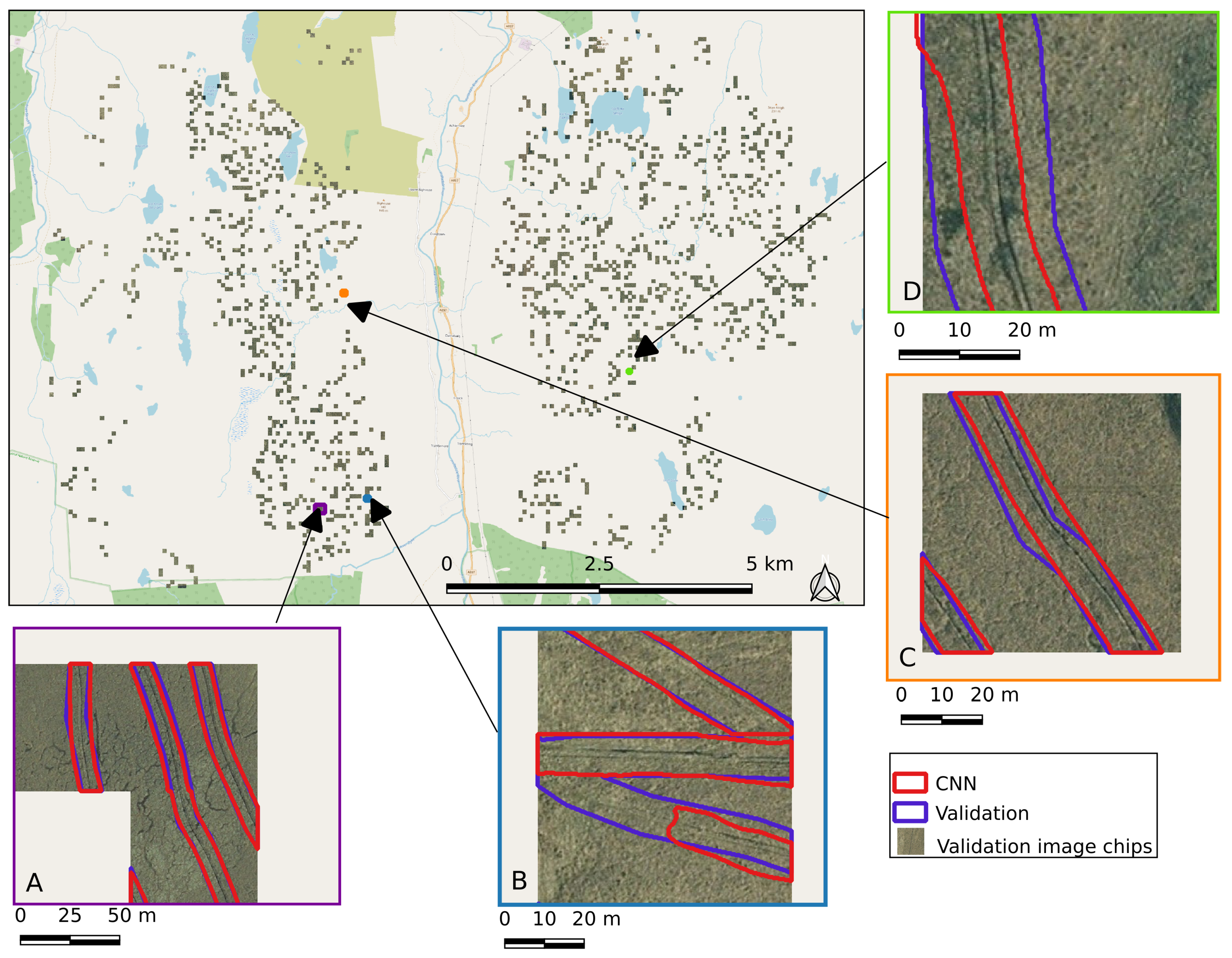
Validation results are displayed in Figure 5, with validation polygons in blue and CNN results in red.
Visual inspection of the validation results reveals well-approximated peat ditch banks and channels, with minor deviations from the validation data of both under- and over-segmentation (Figure 5). Errors of commission and omission are 0.13 and 0.27, respectively, indicating a greater tendency towards under-segmentation. A precision score of 0.87 or commission error of 0.13 indicates that most peat ditches were correctly segmented, with only occasional over-segmentation, such as minor deviations evident in each of the selected panels (Figure 5A–D). A recall score of 0.73 and an omission error of 0.27 indicate that most peat ditches were correctly segmented, with only occasional under-segmentation. Some instances of under-segmentation are evident with the omission of half a channel in Figure 5B and reduced channel bank in Figure 5D. The CNN results here often follow the channel more faithfully/evenly than the manually mapped reference (Figure 5A,C), so the recall score likely under-represents the mapping accuracy.
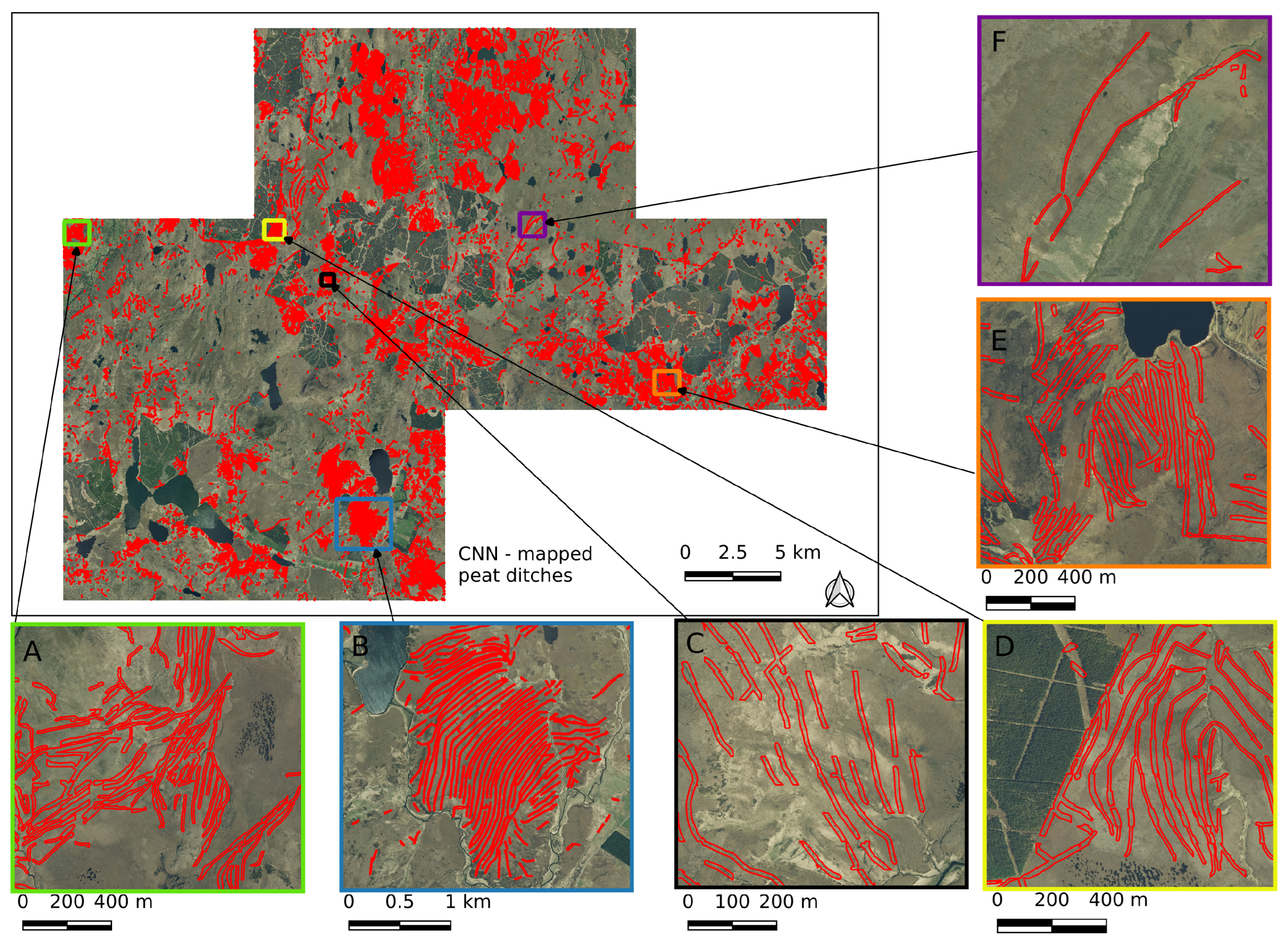
A total of 27,905 peat ditch features were mapped across the study area, the extent of which is depicted in Figure 6, with selected inset details.
Dense areas of peat drainage channels are evident throughout, examples of which are depicted in Figure 6 insets A–E, as well as more isolated examples (Figure 6 inset F). Field-based validation data were not available for the wider study area, although some comments can be made on what appear to be correct mapping and false positives. Drainage ditches were mapped not only in areas of blanket bog vegetation, but also along the margins of forest plantation (Figure 6D). In large part, natural water courses were omitted (i.e., they were not wrongly identified as ditches). Some other linear features such as dry stone walls and water logged tracks were erroneously mapped.
4. Discussion
4.1. Reference Data and Classification Accuracy
The adaptation of the polyline-based training data to an areal representation necessitated a qualitative judgement of the buffer width used to encapsulate each peat-drain. Whilst there are sensible limitations to the choice of width, a minimum is more difficult to estimate given the variation in channel width and the accuracy with which they were mapped. The width chosen was a compromise of both, which may have affected model results, as some portions of training and reference data did not follow the drainage channels accurately.
A U-net-based model was a logical choice given its biomedical origins, where imagery is fixed-perspective, and it is a well-used basis of other remote sensing studies [23] and benchmark dataset contests [37]. A custom built structure may have been a viable alternative, save for the relative lack of training samples.
The F1 score of 0.79 indicates that most ditches were segmented correctly when compared to the reference data. Some omissions resulted, as the channel line was barely visible in the imagery (Figure 5B), due to bank vegetation obscuring the channel, leading to a lack of strong image gradients likely required by the CNN. Whilst independently collected on a different project, the data used for training and validation at times fell short of delineating peat ditch channels faithfully, which affected the recall metric, with a tendency towards under-segmentation. Visual inspection suggests that in many cases, the CNN results actually followed the peat ditch channels more evenly than the reference data, with the implication that the recall score is in fact an under-representation of performance in many cases (Figure 5A,C). An encouraging aspect of this finding is that despite often imprecise training data, the CNN still performed well overall. This reinforces the need for an automated method, rather than field- or desk-based manual methods which are at greater risk of subjective assessment. Furthermore, for peat ditch blocking efforts, only the approximate location of the channels are required, so the results could be readily usable in an applied context with prior manual checking. Within the test set, some errors of commission were attributable to the limitations of the field-based verification data, though there were cases where the CNN-based segmentation was less faithful to the channel and banks (Figure 5D). In the wider study area, extensive areas of peat ditches were mapped successfully, whether chaotically distributed (Figure 6A), systematic (Figure 6B–D), or more isolated (Figure 6E). Drainage channels were also mapped in areas of active forest plantation and immediately adjacent to roads and railways, suggesting that differing background noise does not have a major effect on the CNN detections. Plantation-based detections were limited to the main water-filled drainage lines, whereas the dense, linear ditches between windrows in felled plantations were omitted. Erroneously mapped peat ditches in the wider area included objects such as water-logged vehicle tracks, stone walls, and some isolated areas of railway line provides some insight into the response patterns within the network. These are linear features, where a sharp change in image gradient occurs, likely features generated within the network encoder. CNN-mapping of drainage ditches as outlined in this study provides a robust measure of ditch presence and extent, but not condition. For example, it is not possible to differentiate whether a ditch partially infilled with vegetation still has active flow. The same applies to ditches mapped manually from aerial imagery. Consequently, further field validation will always be required to determine condition and restoration needs.
From an imagery interpretation perspective, the Flow Country is a relatively uniform landscape, making it an ideal test area for CNN-based ditch mapping. Other smaller and less remote blanket bogs, with more varied landscape features, may require more training; therefore a future objective is to test the method in other areas of the UK. The method would also benefit from testing on other peatland types, such as lowland raised bogs and fens, and from application to drainage-impacted peatland regions internationally.
4.2. Comparison with Other Studies
A number of studies, such as [12,19], make use of remotely sensed data in mapping peat land features but employ manual methods to extract them. Therefore, few studies are available to make a comparison with our results, particularly with the use of optical data. Connolly and Holden [16] is most similar from the perspective of input data but uses a semi-manual approach where the target areas are manually constrained, intermediate results are corrected, and peat ditches are of an exclusively uniform pattern. Given the level of manual intervention in [16], a direct comparison of accuracy with this study is of limited value. In non-peatland contexts, LiDAR-based studies used either a rule-based [14,17] or supervised machine learning approach [13,15,18] to extract drainage ditches. Each of these studies were conducted in relatively small, well-constrained, level agrarian landscapes. Where available, the addition of sub-metre-resolution LiDAR or photogrammetry-derived (e.g., UAV-derived) elevation data may serve to improve our results, but the collection of these data is at present sporadic or of insufficient resolution in the UK. The use of optical data from UAVs or sub-metre resolution satellite imagery are also future consideration for applying a CNN-based approach.
5. Conclusions
Information on the location and extent of drainage features on UK peatlands is surprisingly poor, representing a key evidence gap for national emissions inventory reporting [10] and a barrier to effective peatland conservation and restoration. Manual mapping of the areas involved is not feasible, and automated approaches to date have produced mixed results or been reliant on expensive, small-scale data such as high-resolution LiDAR. The results of our study suggest that ditches can be accurately mapped based on existing aerial imagery and a relatively small training set, offering a potentially scalable and affordable solution. If shown to be effective in other UK blanket bogs, this approach may also have potential for mapping other peatland types, both in the UK and internationally. Notably, the promising performance of the CNN method near conifer plantations suggest that it may be suitable for application to other forested peatland regions. For example, an estimated 7.7 million hectares of peat swamp forests in Indonesia and Malaysia have been drained for agriculture and forestry, mostly since 1990, with huge implications for global CO emissions and biodiversity [38]. Many areas are inaccessible, land-use change is rapid and ongoing, and ground-based mapping is sparse, so the capacity to detect the presence of ditches using an automated remote sensing approach would have high value. Given that drained and degraded peatlands are believed to be responsible for 4% of UK GHG emissions [10], and a similar proportion of global GHG emissions [39], this capacity is urgently needed if countries are to achieve their climate-change-mitigation goals.
Author Contributions
Conceptualization, C.R., J.L.W., A.P. and A.F.; methodology, C.R.; software, C.R.; validation, C.R.; formal analysis, C.R.; investigation, C.R.; resources, C.R.; data curation, C.R., J.L.W., A.P. and A.F.; writing—original draft preparation, C.R., J.L.W., A.P. and C.E.; writing—review and editing, C.R., J.L.W. and A.P.; visualization, C.R.; supervision, C.R., J.L.W. and A.P.; project administration, A.P.; funding acquisition, A.P. All authors have read and agreed to the published version of the manuscript.
Funding
This research was funded by the Natural Environment Research Council as part of the Land Ocean Carbon Transfer (LOCATE) project. UK Centre for Ecology and Hydrology grant number NEC05686.
Data Availability Statement
The results of this study are available on request.
Acknowledgments
The authors would like to thank NatureScot for the use of ditch mapping data collected in the Flow Country as part of the PEATLAND ACTION project. A.F. and J.L.W. would like to thank Thom Kirwan-Evans for their time investigating the feasibility of a machine learning approach for peat ditch detection.
Conflicts of Interest
The authors declare no conflict of interest.
Abbreviations
The following abbreviations are used in this manuscript:
| GHG | Greenhouse gas |
| DOC | Dissolved Organic Carbon |
| POC | Particulate Organic Carbon |
| LiDAR | Light Detection and Ranging |
| ML | Machine Learning |
| CNN | Convolutional Neural Net |
References
- Leifeld, J.; Wüst-Galley, C.; Page, S. Intact and managed peatland soils as a source and sink of GHGs from 1850 to 2100. Nat. Clim. Chang. 2019, 9, 945–947. [Google Scholar] [CrossRef]
- Joosten, H.; Sirin, A.; Couwenberg, J.; Laine, J.; Smith, P. The role of peatlands in climate regulation. In Peatland Restoration and Ecosystem Services: Science, Policy and Practice; Bonn, A., Allott, T., Evans, M., Joosten, H., Stoneman, R., Eds.; Ecological Reviews; Cambridge University Press: Cambridge, UK, 2016; pp. 63–76. [Google Scholar] [CrossRef]
- Evans, C.D.; Peacock, M.; Baird, A.J.; Artz, R.R.; Burden, A.; Callaghan, N.; Chapman, P.J.; Cooper, H.M.; Coyle, M.; Craig, E.; et al. Overriding water table control on managed peatland greenhouse gas emissions. Nature 2021, 593, 548–552. [Google Scholar] [CrossRef] [PubMed]
- Sirin, A.; Medvedeva, M.; Korotkov, V.; Itkin, V.; Minayeva, T.; Ilyasov, D.; Suvorov, G.; Joosten, H. Addressing peatland rewetting in Russian federation climate reporting. Land 2021, 10, 1200. [Google Scholar] [CrossRef]
- Bain, C.G.; Bonn, A.; Stoneman, R.; Chapman, S.; Coupar, A.; Evans, M.; Gearey, B.; Howat, M.; Joosten, H.; Keenleyside, C.; et al. IUCN UK Commission of Inquiry on Peatlands; IUCN UK Peatland Programme: Edinburgh, UK, 2011. [Google Scholar]
- Artz, R.; Evans, C.; Crosher, I.; Hancock, M.; Scott-Campbell, M.; Pilkington, M.; Jones, P.; Chandler, D.; McBride, A.S.; Ross, K.F.C.; et al. Commission of Inquiry on Peatlands: The State of UK Peatlands—An Update; Technical Report September; James Hutton Institute: Aberdeen, UK, 2019. [Google Scholar]
- Williamson, J.; Rowe, E.; Reed, D.; Ruffin, L.; Jones, P.; Dolan, R.; Buckingham, H.; Jones, P.; Astbury, S.; Evans, C.D. Historical peat loss explains limited short-term response of drained blanket bogs to rewetting. J. Environ. Manag. 2017, 188, 278–286. [Google Scholar] [CrossRef] [Green Version]
- Parry, L.E.; Holden, J.; Chapman, P.J. Restoration of blanket peatlands. J. Environ. Manag. 2014, 133, 193–205. [Google Scholar] [CrossRef] [Green Version]
- Evans, C.D.; Renou-Wilson, F.; Strack, M. The role of waterborne carbon in the greenhouse gas balance of drained and re-wetted peatlands. Aquat. Sci. 2016, 78, 573–590. [Google Scholar] [CrossRef] [Green Version]
- Evans, C.; Artz, R.; Moxley, J.; Smyth, M.A.; Taylor, E.; Archer, N.; Burden, A.; Williamson, J.; Donnelly, D.; Thomson, A.; et al. Implementation of an Emissions Inventory for UK Peatlands; Technical Report 1; UK Centre for Ecology and Hydrology: Lancaster, UK, 2017. [Google Scholar]
- UK Centre for Ecology and Hydrology; Element Energy. Greenhouse Gas Removal Methods and Their Potential UK Deployment; Technical Report October; UK Centre for Ecology and Hydrology Element Energy: Lancaster, UK, 2021. [Google Scholar]
- Carless, D.; Luscombe, D.J.; Gatis, N.; Anderson, K.; Brazier, R.E. Mapping landscape-scale peatland degradation using airborne lidar and multispectral data. Landsc. Ecol. 2019, 34, 1329–1345. [Google Scholar] [CrossRef] [Green Version]
- Bryn, A.; Dramstad, W.; Fjellstad, W. Mapping and density analyses of drainage ditches in Iceland. In Proceedings of the Mapping and Monitoring of Nordic Vegetation and landscapes, Hverageroi, Iceland, 16–18 September 2009; Norsk Institutt for Skog og Landskap: Steinkjer, Norway, 2010; pp. 43–45. [Google Scholar]
- Cazorzi, F.; Fontana, G.D.; Luca, A.D.; Sofia, G.; Tarolli, P. Drainage network detection and assessment of network storage capacity in agrarian landscape. Hydrol. Process. 2013, 27, 541–553. [Google Scholar] [CrossRef]
- Bailly, J.S.; Lagacherie, P.; Millier, C.; Puech, C.; Kosuth, P. Agrarian landscapes linear features detection from LiDAR: Application to artificial drainage networks. Int. J. Remote Sens. 2008, 29, 3489–3508. [Google Scholar] [CrossRef]
- Connolly, J.; Holden, N.M. Detecting peatland drains with Object Based Image Analysis and Geoeye-1 imagery. Carbon Balance Manag. 2017, 12, 7. [Google Scholar] [CrossRef] [Green Version]
- Rapinel, S.; Hubert-Moy, L.; Clément, B.; Nabucet, J.; Cudennec, C. Ditch network extraction and hydrogeomorphological characterization using LiDAR-derived DTM in wetlands. Hydrol. Res. 2015, 46, 276–290. [Google Scholar] [CrossRef]
- Roelens, J.; Höfle, B.; Dondeyne, S.; Van Orshoven, J.; Diels, J. Drainage ditch extraction from airborne LiDAR point clouds. ISPRS J. Photogramm. Remote Sens. 2018, 146, 409–420. [Google Scholar] [CrossRef]
- Artz, R.R.E.; Donaldson-Selby, G.; Poggio, L.; Donnelly, D.; Aitkenhead, M. Comparison of Remote Sensing Approaches for Detection of Peatland Drainage in Scotland; Technical Report; The James Hutton Institute: Aberdeen, UK, 2017. [Google Scholar]
- Waldner, F.; Diakogiannis, F.I. Deep learning on edge: Extracting field boundaries from satellite images with a convolutional neural network. Remote Sens. Environ. 2020, 245, 111741. [Google Scholar] [CrossRef]
- Ronneberger, O.; Fischer, P.; Brox, T. U-Net: Convolutional Networks for Biomedical Image Segmentation. In Proceedings of the 18th International Conference on Medical Image Computing and Computer-Assisted Intervention, Munich, Germany, 5–9 October 2015; pp. 234–241. [Google Scholar] [CrossRef] [Green Version]
- Falk, T.; Mai, D.; Bensch, R.; Çiçek, Ö.; Abdulkadir, A.; Marrakchi, Y.; Böhm, A.; Deubner, J.; Jäckel, Z.; Seiwald, K.; et al. U-Net: Deep learning for cell counting, detection, and morphometry. Nat. Methods 2019, 16, 67–70. [Google Scholar] [CrossRef] [PubMed]
- Kattenborn, T.; Eichel, J.; Fassnacht, F.E. Convolutional Neural Networks enable efficient, accurate and fine-grained segmentation of plant species and communities from high-resolution UAV imagery. Sci. Rep. 2019, 9, 17656. [Google Scholar] [CrossRef] [Green Version]
- Chen, L.C.; Papandreou, G.; Kokkinos, I.; Murphy, K.; Yuille, A.L. DeepLab: Semantic Image Segmentation with Deep Convolutional Nets, Atrous Convolution, and Fully Connected CRFs. IEEE Trans. Pattern Anal. Mach. Intell. 2018, 40, 834–848. [Google Scholar] [CrossRef] [Green Version]
- Krizhevsky, A.; Sutskever, I.; Hinton, G.E. ImageNet Classification with Deep Convolutional Neural Networks. In Proceedings of the Advances in Neural Information Processing Systems, Lake Tahoe, NV, USA, 3–6 December 2012; Pereira, F., Burges, C.J.C., Bottou, L., Weinberger, K.Q., Eds.; Curran Associates, Inc.: Red Hook, NY, USA, 2012; Volume 25. [Google Scholar]
- He, K.; Gkioxari, G.; Dollar, P.; Girshick, R. Mask R-CNN. In Proceedings of the IEEE International Conference on Computer Vision, Venice, Italy, 22–29 October 2017; pp. 2980–2988. [Google Scholar] [CrossRef]
- He, K.; Zhang, X.; Ren, S.; Sun, J. Deep residual learning for image recognition. In Proceedings of the IEEE Computer Society Conference on Computer Vision and Pattern Recognition, Las Vegas, NV, USA, 27–30 June 2016; pp. 770–778. [Google Scholar] [CrossRef]
- Zhang, C.; Atkinson, P.M.; George, C.; Wen, Z.; Diazgranados, M.; Gerard, F. Identifying and mapping individual plants in a highly diverse high-elevation ecosystem using UAV imagery and deep learning. ISPRS J. Photogramm. Remote Sens. 2020, 169, 280–291. [Google Scholar] [CrossRef]
- Lindsay, R.; Charman, D.J.; Everingham, F.; Reilly, R.M.O.; Palmer, M.A.; Rowell, T.A.; Stroud, D.A.; Ratcliffe, D.A.; Oswald, P.H.; O’Reilly, R.M.; et al. The Flow Country—The peatlands of Caithness and Sutherland; Technical Report; Joint Nature Conservation Committee: Peterborough, UK, 1988. [Google Scholar]
- Alshammari, L.; Large, D.J.; Boyd, D.S.; Sowter, A.; Anderson, R.; Andersen, R.; Marsh, S. Long-term peatland condition assessment via surface motion monitoring using the ISBAS DInSAR technique over the Flow Country, Scotland. Remote Sens. 2018, 10, 1103. [Google Scholar] [CrossRef] [Green Version]
- Robb, C. Geospatial-Learn; Zenodo: Geneve, Switzerland, 2017. [Google Scholar] [CrossRef]
- Virtanen, P.; Gommers, R.; Oliphant, T.E.; Haberland, M.; Reddy, T.; Cournapeau, D.; Burovski, E.; Peterson, P.; Weckesser, W.; Bright, J.; et al. SciPy 1.0: Fundamental Algorithms for Scientific Computing in Python. Nat. Methods 2020, 17, 261–272. [Google Scholar] [CrossRef] [Green Version]
- Pedregosa, F.; Varoquaux, G.; Gramfort, A.; Michel, V.; Thirion, B.; Grisel, O.; Blondel, M.; Louppe, G.; Prettenhofer, P.; Weiss, R.; et al. Scikit-learn: Machine Learning in Python. J. Mach. Learn. Res. 2012, 12, 2825–2830. [Google Scholar] [CrossRef]
- GDAL OGR Contributors. {GDAL/OGR} Geospatial Data Abstraction Software Library; Open Source Geospatial Foundation: Beaverton, OR, USA, 2020. [Google Scholar]
- Paszke, A.; Gross, S.; Massa, F.; Lerer, A.; Bradbury, J.; Chanan, G.; Killeen, T.; Lin, Z.; Gimelshein, N.; Antiga, L.; et al. PyTorch: An Imperative Style, High-Performance Deep Learning Library. In Advances in Neural Information Processing Systems 32; Wallach, H., Larochelle, H., Beygelzimer, A., d’Alché-Buc, F., Fox, E., Garnett, R., Eds.; Curran Associates, Inc.: Red Hook, NY, USA, 2019; pp. 8024–8035. [Google Scholar]
- Buslaev, A.; Parinov, A.; Khvedchenya, E.; Iglovikov, V.I.; Kalinin, A.A. Albumentations: Fast and flexible image augmentations. Information 2020, 11, 125. [Google Scholar] [CrossRef] [Green Version]
- Maggiori, E.; Tarabalka, Y.; Charpiat, G.; Alliez, P. Can Semantic Labeling Methods Generalize to Any City? The Inria Aerial Image Labeling Benchmark. In Proceedings of the IEEE International Geoscience and Remote Sensing Symposium (IGARSS), Fort Worth, TX, USA, 23–28 July 2017. [Google Scholar]
- Wijedasa, L.S.; Sloan, S.; Page, S.E.; Clements, G.R.; Lupascu, M.; Evans, T.A. Carbon emissions from South-East Asian peatlands will increase despite emission-reduction schemes. Glob. Chang. Biol. 2018, 24, 4598–4613. [Google Scholar] [CrossRef] [PubMed]
- Smith, P.; Clark, H.; Dong, H.; Elsiddig, E.A.; Haberl, H.; Harper, R.; House, J.; Jafari, M.; Masera, O.; Mbow, C.; et al. Agriculture, Forestry and Other Land Use (AFOLU). In Mitigation of Climate Change. Contribution of Working Group III to the Fifth Assessment Report of the Intergovernmental Panel on Climate Change; Edenhofer, O., Pichs-Madruga, R., Sokona, Y., Farahani, E., Kadner, S., Seyboth, K., Adler, A., Baum, I., Brunner, S., Eickemeier, P., et al., Eds.; Cambridge University Press: Cambridge, UK, 2014; pp. 811–922. [Google Scholar] [CrossRef]
Figure 1.
The study area in local, regional and national contexts, with manually mapped peat ditches in blue. Basemap layers are provided by Open Street Map using the HCMGIS (v.22.9.9) QGIS plugin.
Figure 1.
The study area in local, regional and national contexts, with manually mapped peat ditches in blue. Basemap layers are provided by Open Street Map using the HCMGIS (v.22.9.9) QGIS plugin.

Figure 2.
Subsection of the training data with insets from top to bottom consisting of digitised polylines (blue) and 5 m buffered polygons (red) and the underlying images with peat ditches visible.
Figure 2.
Subsection of the training data with insets from top to bottom consisting of digitised polylines (blue) and 5 m buffered polygons (red) and the underlying images with peat ditches visible.

Figure 3.
A sample of dehidral augmentations employed on each training chip, with imagery (top) and corresponding masks (bottom).
Figure 3.
A sample of dehidral augmentations employed on each training chip, with imagery (top) and corresponding masks (bottom).

Figure 4.
Schematic of the CNN architecture, with the input image (see Figure 3), encoder, bottleneck, decoder and binary output from left to right. Yellow panels represent the feature layers, red the max pooling operations, and blue the up-convolutions.
Figure 4.
Schematic of the CNN architecture, with the input image (see Figure 3), encoder, bottleneck, decoder and binary output from left to right. Yellow panels represent the feature layers, red the max pooling operations, and blue the up-convolutions.

Figure 5.
Validation results, with the spatial distribution of validation data held separate from the training and test sets displayed in the main map panel, with selected examples insets labelled (A–D). Validation polygons are blue and CNN polygons are red.
Figure 5.
Validation results, with the spatial distribution of validation data held separate from the training and test sets displayed in the main map panel, with selected examples insets labelled (A–D). Validation polygons are blue and CNN polygons are red.

Figure 6.
CNN-based mapping results with colour-coded detail insets.


Table 1.
Precision, recall, and scores.
| Stage | Precision | Recall | F |
|---|---|---|---|
| Validation | 0.87 | 0.73 | 0.79 |
Disclaimer/Publisher’s Note: The statements, opinions and data contained in all publications are solely those of the individual author(s) and contributor(s) and not of MDPI and/or the editor(s). MDPI and/or the editor(s) disclaim responsibility for any injury to people or property resulting from any ideas, methods, instructions or products referred to in the content. |
© 2023 by the authors. Licensee MDPI, Basel, Switzerland. This article is an open access article distributed under the terms and conditions of the Creative Commons Attribution (CC BY) license (https://creativecommons.org/licenses/by/4.0/).
Share and Cite
MDPI and ACS Style
Robb, C.; Pickard, A.; Williamson, J.L.; Fitch, A.; Evans, C. Peat Drainage Ditch Mapping from Aerial Imagery Using a Convolutional Neural Network. Remote Sens. 2023, 15, 499. https://doi.org/10.3390/rs15020499
AMA Style
Robb C, Pickard A, Williamson JL, Fitch A, Evans C. Peat Drainage Ditch Mapping from Aerial Imagery Using a Convolutional Neural Network. Remote Sensing. 2023; 15(2):499. https://doi.org/10.3390/rs15020499
Chicago/Turabian StyleRobb, Ciaran, Amy Pickard, Jennifer L. Williamson, Alice Fitch, and Chris Evans. 2023. "Peat Drainage Ditch Mapping from Aerial Imagery Using a Convolutional Neural Network" Remote Sensing 15, no. 2: 499. https://doi.org/10.3390/rs15020499
Note that from the first issue of 2016, this journal uses article numbers instead of page numbers. See further details here.