Short-Term Ecogeomorphic Evolution of a Fluvial Delta from Hindcasting Intertidal Marsh-Top Elevations (HIME)


1
Princeton Hydro, Ringoes, NJ 08551, USA
2
School of the Environment, Washington State University, Vancouver, WA 98686, USA
3
Department of Geological Sciences, The University of Texas at Austin, Austin, TX 78712–1722, USA
*
Author to whom correspondence should be addressed.
Remote Sens. 2020, 12(9), 1517; https://doi.org/10.3390/rs12091517
Submission received: 16 March 2020
/
Revised: 21 April 2020
/
Accepted: 29 April 2020
/
Published: 9 May 2020
(This article belongs to the Special Issue Remote Sensing of Estuarine, Lagoon and Delta Environments)
Abstract
:Understanding how delta islands grow and change at contemporary, interannual timescales remains a key scientific goal and societal need, but the high-resolution, high frequency morphodynamic data that would be most useful for this are as yet logistically prohibitive. The recorded water levels needed for relative elevation analysis are also often lacking. This paper presents a new approach for hindcasting intertidal marsh-top elevations (HIME) to resolve ecogeomorphic change, even in a young, rapidly changing fluvial delta setting, at sub-decadal temporal resolution and at the spatial resolution of widely available optical remote sensing imagery (e.g., 30 m Landsat). The HIME method first calculates: (i) the probability of land exposure in a set of historical imagery from a user-defined discrete timespan (e.g., months or years); (ii) the probability of water level non-exceedance from water level records, which need not be complete nor coincident with the imagery; and (iii) the systematic variation in local mean water level with distance along the primary hydraulic gradient. The HIME method then combines these inputs to estimate a marsh-top elevation map for each historical timespan of interest. The method was developed, validated, applied, and results analyzed to investigate time-lapse evolution of the Wax Lake Delta in Louisiana, USA, every three years, over two decades (1993–2013). The hindcast maps of delta island extents and elevations evidenced ecogeomorphic system self-organization around four stable attractors, or elevation platforms, at about −0.3 m (subtidal), 0.2 m, 0.4 m, and 0.9 m (supratidal) NAVD88. The HIME results also yielded a time series of net subaerial sediment accumulation, and specific locations and magnitudes of gains and losses, at scales from 30 m to delta-wide (~100 km3) and 6 to 21 years. Average subaerial net sediment accumulation at the Wax Lake Delta (WLD) was estimated as 0.6 cm/yr during the study period. Finally, multiple linear regression models were successfully trained on the HIME elevation maps to model evolving delta island morphologies based on simple geometric factors, such as distance down-delta and position on a delta island; the models also successfully reproduced an average delta topset slope of 1.4 cm. Overall, this study’s development and application of the HIME method added detailed insights to recent, transient ecogeomorphological change at the WLD, and demonstrated the potential of the new approach for accurately reconstructing past intertidal topographies and dynamic change.
1. Introduction
Surface elevation is a geomorphologically and ecologically important variable in fluvial, floodplain, tidal, marsh, and delta environments. Sediment elevations high enough to experience regular subaerial exposure facilitate vegetation colonization. Enhanced vegetation growth and lateral vegetation expansion help stabilize sediments. Vegetation further aids sediment trapping at, and accretion to, the elevations suitable for its growth, closing the loop of a sediment-vegetation eco-geomorphological positive feedback. Sediment erosion between vegetation patches makes eroding areas less hospitable for vegetation colonization, while also providing part of the sediment source for nearby accumulation among vegetation, forming a second positive feedback loop, but in the opposite sense. Together, these two linked ecogeomorphological feedbacks are thought to create “stable attractors” of marsh elevation, i.e., elevations to which marshes will accrete, from slightly lower elevations, or erode, from slightly higher elevations. When sufficiently strong, these feedbacks lead to a wetland system self-organizing into discrete and spatially contrasting (i.e., patterned) vegetated and non-vegetated areas, or multiple vegetated and non-vegetated sediment platforms. Mathematically, the balance of accretion and erosion at a stable attractor should satisfy the condition that the vertical rate of elevation change over time is zero, i.e., dz/dt ≈ 0. Geomorphic stable attractors have therefore been diagnosed empirically by the resulting symptom of sediment accumulation at specific (attractor) marsh elevations and loss at intervening (erosional) elevations. This theory and various empirical cases of these phenomena were reviewed for tidal wetlands by Moffett et al. (2015) [1] and the feedback mechanisms thoroughly synthesized across fluvial and wetland settings by Larsen (2019) [2]. Although now fairly widely adopted to describe quiescent freshwater and saline tidal marsh settings, it is not yet clear if strongly advective fluvial settings, such as a young, prograding fluvial delta, can similarly exhibit eco-geomorphological elevation differentiation, especially over the short interannual to decadal timescales one might think to be dominated by strong exogenous forcing, such as hurricanes and major river floods [3,4,5,6].
For a young, rapidly prograding delta, island formation initially occurs subaqueously, governed by hydrodynamics and aqueous sediment transport. Flow expansion and deceleration where channelized flow transitions into a larger body of water induce sediment deposition, forming a mouth bar [7,8]. The location of the mouth bar, which sets the initial location for island formation, is strongly controlled by water velocity and depth and weakly controlled by grain size [8,9]. Field studies suggest that this jet deposit model initiates mounded island forms, with their thickest deposits at the upstream end and along the central island axis [10]. Flow splitting around the mouth bar causes channel bifurcation and levee development behind the bar [8,9]. Deltas exhibit strong morphodynamic coupling between surface elevation, water flow, and sediment deposition or erosion [11,12]. Bed or bar elevation controls the depth and frequency of inundation, which in turn affect bed shear stress and the amount and type of sediment available for deposition at a given location [13,14,15]. These processes are reviewed by Fagherazzi et al. (2015) [16], broader delta-forming processed by Ericson et al. (2006) [17], and specific mechanisms of delta sedimentation by Olliver et al. (2020) [18].
Once delta bars accrete to a level near or above mean water level, emergent plants are able to colonize the nascent islands. Wetland vegetation increases net mineral sedimentation by increasing bed roughness, slowing water velocity, and decreasing eddy diffusivity, thereby promoting particle settling and decreased resuspension [19,20,21]. Studies in non-delta marshes have correlated sedimentation rates with vegetation cover, though elevation and proximity to tidal channels are also factors [22,23]; results have been highly variable [24]. For example, if vegetation density, roughness, or height is sufficient to limit flow and transport across the marsh platform, vegetation can have an opposite, sediment-excluding, effect on wetland islands [18,25]. Cohesive and non-cohesive sediments may also exhibit contrasting behavior with respect to vegetation density and fluvial discharge: non-cohesive sediment accumulation may decrease with increased vegetation density and be insensitive to discharge, whereas cohesive sediment accumulation may increase with increased vegetation density and slightly decrease with increased discharge [25]. These conundrums further inspire this study to investigate whether a young, prograding fluvial delta setting, especially one with a high sand fraction among its sediment load, can self-organize according to multiple stable eco-geomorphological attractors, in reality, or whether at short, inter-annual to decadal timescales, exogenous forces will overwhelm local vegetation-sedimentation feedback mechanisms.
If eco-geomorphological feedbacks are successful at stabilizing and helping to endogenously organize delta marshes, the combination of trapping and erosive feedbacks should lead to self-perpetuating sediment platforms at the discrete elevations of the eco-geomorphological stable attractor(s). A system may theoretically exhibit bi-stable states, i.e., simultaneously attract at different spatial locations within the domain of interest to one high and one low elevation; or a system may exhibit multiple stable states, with more than two stable attractors, each expressed simultaneously at different locations in the study domain. Note, herein we use the wording “multiple stable attractors” to refer to the co-existence of several discrete elevation platforms at different locations within one study domain, i.e., different marsh elevations reinforced by sediment-vegetation feedbacks among several vegetation species; this contrasts with the term “alternative stable states,” which we would reserve for describing potentially interchangeable but catastrophic whole-ecosystem shifts of the entire study domain of interest, e.g., subaerial marshland fully collapsing to subaqueous mudflat or two completely alternative patterns of ecosystem self-organization [1,26].
Although widely explored in theoretical models and in select studies of intertidal salt marshes, mangroves, mudflats, and mussel beds [1], only a few studies have yet tested the possibility of fluvial deltas expressing multiple stable eco-geomorphological states. All such studies that we were able to find have used the young Wax Lake Delta (WLD) near Morgan City, Louisiana, USA as the focus of investigation. Olliver and Edmonds (2017) used optical remote sensing data and field surveying to identify two stable states at the WLD, low elevation water and high elevation marsh, and the “land building succession” between them, via which water converted to marsh over time (1985–2015) [27]. Wagner et al. (2017) identified two intermediate-elevation platforms and one geomorphic stable attractor (dz/dt = 0), based on WLD elevation changes between 2009 and 2013 LIDAR surveys [28]. Ma et al. (2018) found three elevation/vegetation zones that expressed different relations between elevation and LIDAR-derived biomass volume [29]. Data from a few additional studies may also indirectly suggest multiple stable states: Bevington and Twilley’s (2018) findings of at least two discrete elevations of contrasting soil organic matter accumulation [30], O’Connor and Moffett’s (2015) notes of at least two different elevation platforms with contrasting vegetation zones and sediment properties [31], and Carle et al. (2015) clearly mapping several distinct elevation-aligned vegetation zones at WLD [32]. A broader review of WLD geomorphic and research history is provided by Twilley et al. (2019) [33].
While one would wish to have topographic data at high spatial resolution to resolve narrow individual bars and levees, at high temporal resolution to resolve sometimes rapid morphometric change, and continuously over sufficient duration of time (e.g., weeks to decades, or longer) to observe dynamic system evolution, the insights into the possibility of multiple stable ecogeomorphological states in a young fluvial delta have so far relied on creative analyses and innovative interpretations of proxy data for delta marsh elevation change, or data from few points in space or time. Complete morphologic mapping of complex delta geometries in situ, as they evolve in space and time, is usually infeasible at scales to capture dynamic changes before sediment re-working erases key, but temporary, features. In most delta settings it is very challenging to obtain high-precision, high-resolution, frequently-repeated empirical measures of surface topography [34]. Terrestrial light detection and ranging (LIDAR) scanning cannot efficiently cover the system-wide spatial extents needed, and airborne LIDAR data tend to be expensively and infrequently obtained. Manual methods are laborious, although stratigraphic studies assemble such perspectives on deltaic change over timescales spanning decades to millennia (e.g., [35,36,37,38,39,40]). Stratigraphic approaches, however, even applied to modern sediment cores, are unable to resolve short-term morphodynamics of unconsolidated sediments, which may alternately accrete and erode over several unpreserved cycles before ultimately recording the net result as a preserved stratum. A very promising approach of mapping dynamic floods and relative topographic change has been recently pioneered using stacks of space-borne microwave synthetic aperture radar (SAR) imagery [41,42], although at too coarse a spatial scale to resolve detailed delta morphodynamics, and so far reliant on external elevation mapping (e.g., coarse global shuttle radar topography) to place results vertically. In the future, additional advances may become feasible from high-resolution satellite laser altimetry, SAR, or routine airborne LIDAR, but to date, technology has not been available to produce the desired abundant, rich, frequent, high-resolution topographic data needed to study short-term but extensive marsh geomorphic change.
To help fill the gap of high spatial and temporal resolution topographic mapping of wetland environments, this study developed a new method to estimate the historical topography of intermittently flooded marshlands based on optical remote sensing data. We name the method hindcasting intertidal marsh-top elevations (HIME). In brief, the HIME method consists of first calculating: (i) the probability of land exposure in a set of historical imagery from a user-defined discrete timespan (e.g., months or years); (ii) the probability of water level non-exceedance from water level records, which need not be complete nor coincident with the imagery; and (iii) the systematic variation in local mean water level with distance along the primary hydraulic gradient. The HIME method then combines these inputs to estimate a marsh-top elevation map for each historical timespan of interest. The method is conceptually similar to the ‘water-line’ approach by Mason et al. (1995) [43] and to the SAR-stacking approach used by Kuenzer et al. (2013) [41], which was coincidentally developed at the same time as we developed the HIME method. Key innovations of the HIME method are its use of high-resolution satellite imagery (e.g., Landsat, 30 m), its derivation of absolute (not only relative) marsh-top elevations, its ability to use water level data that are incomplete and asynchronous relative to the remotely sensed images, and its applicability to hindcast historical topography as far back as remote sensing imagery distinguishing water from marsh are available, e.g., decades back into the satellite record. Once developed and validated, we applied the new HIME method to the exemplary case of the Wax Lake Delta in Louisiana to help better understand short-term (inter-annual to decadal; 1993–2013) spatiotemporal morphodynamics of young, rapidly changing, fluvial delta marshlands. The following are general research questions:
- Are multiple stable ecogeomorphological states apparent even amid transient, rapidly changing, young delta sediment accumulation patterns?
- ○
- i.e., does sediment accumulate to specific elevations over interannual and decadal timescales? If so, at what elevations, and over how much spatial area?
- How are short-term morphodynamic changes related in space and time to delta island marsh ecosystem organization and vegetation zonation?
- What is the dependency of local morphodynamic change on prior elevation states?
- ○
- i.e., is a given elevation at a given point in time more likely to gain or lose elevation and area over succeeding years and decades?
- How do local, interannual expansions and contractions, accretion and erosion, of individual delta islands add up over a whole delta system and over several decades to provide a net accumulated sediment volume, topset rise, and area expansion of a young prograding delta?
2. Materials and Methods
2.1. Study Area
In 1942, the Wax Lake Outlet Channel was constructed by the U.S. Army Corps of Engineers (USACE), by diverting water from the Atchafalaya River upstream from Morgan City, LA for the purposes of flood control. The USACE Old River Control Structure, located at the convergence of the Red and Mississippi Rivers (Figure 1a), diverts 30% of the combined flow from the Mississippi and Red Rivers to the Atchafalaya River, and the Wax Lake Outlet contains up to 46% of the flow from the Atchafalaya [44]. The Wax Lake Outlet therefore carries up to ~14% of Mississippi Basin discharge. The Wax Lake Delta (WLD) is located where the Wax Lake Outlet flows into Atchafalaya Bay at 29°32′21.85″N, 91°25′50.74″W (Figure 1a). The delta has been developing subaqueously since 1952 and became subaerial after a large flood in 1973 [45]. For a thorough description of the historical hydrology and upstream geomorphology of the Atchafalaya system, the reader is referred to the work of, e.g., Mossa (2016) [46] and to the review by Twilley et al. (2019) [33] on the WLD, generally.
Consisting primarily of sand-rich deposits on top of the original consolidated-mud bay floor, the WLD has prograded into the bay approximately 10 km [45,47]. The delta is a low gradient system, with the entire subaerial portion within 1 m of mean water level [48]. The “subaerial” elevations of the WLD have been taken by previous authors to mean lands above mean low water (−0.04 m NAVD88 [30]), but in this study are taken as any sediment or vegetation area exposed subaerially at any observation time within the study period, which includes some subtidal and some supratidal elevations. The WLD is tidally influenced, with an average tidal amplitude of 60 cm [49], though river discharge and wind also factor into water levels [31,50] (Figure 1b,c). Though the WLD extends into Atchafalaya Bay, it is surrounded by freshwater due to the large volume of water discharging from the Wax Lake Outlet.
Due to its small size, relatively good historical record over the last several decades, and lack of substantial engineering [47], the WLD is an ideal place to study young delta dynamics at sub-decadal scales. The WLD has proven useful in previous geomorphological studies, such as on sediment diversion and marsh restoration potential [12,51,52,53,54,55], (sub)aqueous sediment and channel dynamics and fluxes [56,57,58,59,60,61,62,63], river flood, hurricane, and cold front effects on marsh elevations [5,64,65], and delta sedimentation and lobe progradation [18,66]. The WLD has also yielded insights into delta hydrology, including on surface water residence and connectivity [67,68,69,70], surface water-groundwater interactions [31], and effects of river, floods, tides, wind, hurricanes, and cold fronts on water levels [4,5,31,50,64,65,71,72]. Ecological and biogeochemical studies have used the WLD to assess young delta vegetation succession [3,27,32], sediment trapping or erosion [4,29], and vegetation-sediment feedbacks [25], organic carbon accumulation [73,74,75,76], phosphorus, nitrogen, or metals’ mobility and cycling [67,76,77,78,79,80], and ecological and biogeochemical effects of occasional salinization by sea water [65,81,82]. Finally, the WLD has proven to be a useful test bed for other remote sensing-based innovations: to map plant species [83], quantify wetland biomass [84], improve spectroscopic analysis [85], and map surface water currents and subaqueous channels [86,87]. These prior successes provided confidence that the WLD was an appropriate study area for this research.
2.2. Study Overview
This study was conducted in two parts. In the first part, a statistically-based method was developed for hindcasting intertidal marsh-top elevations (HIME). The method enabled approximating changes in marsh extent and elevation over time amid transient water levels, using only optical remote sensing (Landsat) data, and even if water level data were unavailable, concurrent with each remote sensing image. The HIME method development was conducted using Pintail Island within the WLD as a test case, and using a subset of remote sensing imagery from 1999 to 2010. There is little historical topographic information available for the WLD. This study had access only to one LIDAR dataset at 1 m horizontal resolution, from 14–15 January 2009 [48]. However, there is an extensive set of Landsat satellite imagery available at 30 m horizontal resolution [88]. The HIME approach takes advantage of the fact that water level fluctuations have a large effect on how much subaerial (non-water) area is observed in a remote sensing image at any given time (Figure 1b,c). Each Landsat image was obtained at a different, unknown, water level, so each showed a different extent of the delta area.
Previously, remote sensing techniques have been primarily used in deltaic environments to monitor delta spatial extent and vegetation or land cover, without accounting for the effects of changing water level (e.g., [27,89]). Recent work at the WLD has characterized uncertainty associated with using satellite imagery to measure the horizontal extent of delta land area change over time (e.g., [50,90]), but does not address patterns of vertical change. The one study focused specifically on vertical change on WLD islands, by Bevington and Twilley (2018), used twice-annual field surveys from 2008–2011 of seven transects oriented perpendicularly across island apex mouth-bars or lateral levees, and an analysis of 2012 LIDAR data; the authors assessed contrasts in levee relief (height) and island width, according to transects’ distance up-delta, which was related to increasing island age [30]. Inspired by the work by Bevington and Twilley (2018) [30], and by the careful historical accounting of planform WLD island change by Allen et al. (2012) [90], we aimed to expand on the empirical quantification of historical WLD island change through space and time. Other researchers at other study sites have used a series of satellite images to construct an inundation model, but have been unable to tie it to absolute elevations without a priori elevation data (e.g., [41]), or have required absolute water levels to be known at the time the images were taken [43,91,92]. In the case of WLD, and at most sites worldwide, the specific water levels for each Landsat image are not available, and hydrodynamically predicting water levels in sufficient detail is prohibitive as they are a complex function of river, floods, tides, wind, hurricanes, and cold fronts. Therefore, this study developed a method with a probabilistic approach to use information contained in Landsat imagery to model the likely historical topography of the delta. The method was validated on the Pintail Island test case, using a LIDAR dataset from 2009 [48].
The validated HIME method was then applied throughout the WLD (to 46,494 separate 30 m pixels), and over the two-decade study period 1993–2013, to assess planform change in marsh extent and exposed elevations relative to transient water levels throughout the evolving delta system. Cumulative and incremental changes in apparent subaerial delta sediment volumes and elevations over the two decades were then discussed and placed in relation to other studies mapping WLD eco-geomorphological change and delta dynamics and features in the Mississippi River delta system, more generally.
2.3. Hindcasting Intertidal Marsh-Top Elevation (HIME): Method Development
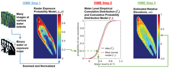
The HIME method consists of 3 main steps, here outlined and further detailed below. The method is also schematically illustrated in Figure 2.
(1) First, a time series of empirical exposure probability models is developed for the region of interest. To do this, a large number of remote sensing images (N) is gathered over the region of interest. Water level change should occur at higher frequency than the morphological changes of interest. The N images are classified into binary maps of water versus non-water (emergent) areas. Areas classified as water are assigned value zero (0) and areas classified as emergent are assigned value one (1). Water is frequently separated from earth and vegetation in optical imagery using the NIR or red bands, which exhibit bimodal distributions in land/water scenes, and the Otsu thresholding method [94] is effective at finding the optimal value(s) to divide a multi-modal histogram into distinct classes (e.g., [95]). We used the Otsu method on the red band (if necessary in RGB-only image) or Band 5 (as recommended by others for distinguishing water in a multiband image [90]) to divide water and non-water pixels. Emergent areas consisted of subaerial sediment or vegetation cover, representing the top of the marsh (“marsh-top”) as viewed from above. Other classification approaches could be adopted without changing the overall sense and framework of the HIME method. As implemented in this study, the HIME method does not distinguish the marsh sediment and vegetation surfaces, but focuses on distinguishing planform island and non-island areas, which is consistent with the most similar prior study of the system, by Allen et al. (2011) [90]. With this approach, the “marsh-top” elevations modeled by the HIME method may be higher than the islands’ sediment-surface elevations; however, the potential magnitude of this and other over- or under-estimations of HIME-modeled marsh elevation compared to true sediment surface elevation were assessed during method validation and found to be less than 0.04 m or <10% (see Section 3.1).
The binary-classified images are then divided into T consecutive temporal subsets (i.e., time intervals i = 1…T), within each of which water extents vary across a wide range of values. The i timeframes, of n images each, need not necessarily be of equal length nor number of images. Within each timeframe, all the binary-classified maps are summed via raster summation. The maximum possible value of this summed map within a given subset is n, if a pixel was non-water in every image, and the minimum possible value zero, if a pixel was water in every image. The summed map is divided by n, resulting in an empirical map of exposure probability pex(i,j) for that timeframe (i) at each pixel (j). Together, these T maps represent a time-lapse series of raster exposure probability models over the whole time period of interest.
(2) Second, a model of water level probability for the study area is developed. Relevant available water level gage data (y) are used to calculate an empirical cumulative distribution function () of the water level probability of non-exceedance (pne). Although this could be used in the analysis directly, in case of discontinuous data our preference was to fit to a continuous distribution function, such as a normal distribution (if appropriate), to obtain a representative model (FY) of the water level cumulative probability of non-exceedance (Pne). In the simplest case, one water level probability model (FY) can be used throughout the region of interest, e.g., if each pixel in the study area is thought to have the same mean and variance of water levels. If instead it is known that there is a background signal not captured in the water level gage data, e.g., a non-zero mean water level slope across the study area due to the water surface slope of a discharging river (as at WLD), or even a known background planar variation in water level, this is added to FY on a pixel-by-pixel basis to create a “map” of FY(j) functions, one for each pixel location (j). Thus, water level probability of non-exceedance models are developed that need not be based on exhaustive or continuous water level input data (y), but that provide an estimate of the local probability of water level non-exceedance (Pne(i,j,Y)) for any water level (Y), at each pixel location (j), and in each timeframe (i), relative to the local mean water level.
(3) Finally, historical marsh-top elevation (zi,j) is hindcast for each timeframe (i) and each pixel (j) within the region and time period of interest. To do so, one first recognizes that the raster exposure probabilities from Step 1 are equivalent to water level non-exceedance probabilities. For example: if a pixel at location j had an exposure probability pex(i,j) = 0.3 from Step 1, then it exhibited a 30% likelihood of being exposed among the n images comprising timeframe i. In other words, we take this as a 30% likelihood of the water being lower than the pixel’s unknown true elevation Z(i,j) during subset timeframe i. This is equivalent to saying that there was a 30% likelihood of water level non-exceedance of elevation Z(i,j) during timeframe i, i.e., that 0.3 = Pne(i,j,Y) for Y= Z(i,j). Therefore, for monotonic FY, one assigns pex(i,j) = Pne(i,j,Y) and inverts Pne(i,j,Y) = FY(j)(Y) to obtain Y, and estimates the unknown, true historical pixel elevation Z(i,j) as the estimated relative elevation z(i,j) = Y. This is shown graphically in Figure 2. Last, the adjustment b(i,j) is applied, if necessary, at each pixel to convert estimated elevations relative to a locally systematically-varying mean water level to the basis of a common fixed datum: z(i,j)MLW + b(i,j) = z(i,j). The HIME method is limited to modeling marsh-top elevations in the range from the lowest water stage to just above the highest water stage imaged among the n images of a during a given timeframe (i). Variations in elevations that are always-emergent in the n images are not distinguished by the HIME method, nor are subaqueous elevations always submerged in the n images of a given timeframe (i).
The following subsections detail and demonstrate these steps of the HIME method, using Pintail Island as an efficient verification example. The same procedure was then applied throughout the WLD to produce the main results of the study, as described below.
2.3.1. HIME Step 1: Marsh Exposure Probability Models, Pintail Island Test Case
To empirically estimate marsh exposure probability for the test case of Pintail Island, we applied Step 1 of the HIME method, as outlined above. Our image database for this test case consisted of N = 79 cloud free Landsat images of the WLD, acquired from the USGS Earth Explorer website for the years 1999–2010, from Path 23, Rows 39 and 40 (Table S1; [88]). Each pixel of each image was classified as emergent marsh-top (=1) or water (=0) surface cover, with no additional pre-processing. The binary-classified maps were then divided into T = 4 consecutive timeframes for the Pintail Island test case, each spanning 3 years: 1999–2001 (i = 1, n = 18), 2002–2004 (i = 2, n = 19), 2005–2007 (i = 3, n = 19), and 2008–2010 (i = 4, n = 24). After summation of the binary-classified maps within each timeframe, and normalization by n, we obtained the time series of raster exposure probability models pex(i,j), covering each timeframe i and pixel location j for Pintail Island (Figure S1).
2.3.2. HIME Step 2: Water Level Models, Pintail Island Test Case
To develop models of the cumulative probability of water level non-exceedance for the test case of Pintail Island, we applied Step 2 of the HIME method. We used as model input (y) the daily-average surface water level data from USGS gage 073815925 [93] at the apex of the delta (29°32′24″N, 91°26′08″W; Figure S2). Data with water level specified were only available for the period 15 October 2008–12 January 2014 at the time of the study. A key innovation of the HIME method, however, is that the available water level data need not necessarily represent a complete record spanning the full range of the imagery time series. Instead, one must only have water level data that sufficiently span the range of high-frequency water level variations expressed in the imagery, to create an informative empirical cumulative probability density function of water level (). The mean surface water level at the gage for this period was 0.48 m NAVD88, reaching a maximum level of 1.12 m and a minimum level of −0.11 m. To provide a continuous function covering all marsh surfaces, the cumulative distribution of water levels throughout the test period was fitted with a normal cumulative distribution function (FY), with a mean of 0.48 m and a standard deviation of 0.21 m (shown in center of Figure 2).
2.3.3. HIME Step 3: Hindcasting Marsh-Top Elevation, Pintail Island Test Case
To combine the historical remote sensing and water level probability data and so hindcast historical marsh-top elevations for the Pintail Island test case, we applied Step 3 of the HIME method, as outlined above. For every pex(i,j) in the raster exposure probability models, the overall FY function relating water level and probability of non-exceedance was used to calculate the water elevation (Y) at which the pixel would flood, i.e., to estimate its marsh surface height above mean low water level (MLW) as z(i,j)MLW = Y. For WLD, FY was modeled relative to MLW because this was the native datum of the Camp Island water level gage. An adjustment was made for map pixels that were never inundated during the imaged times, and so had a value of pex(i,j) = 1, because the inversion of the normal function FY at the value of 1 to obtain an elevation estimate Y would return an apparently infinite elevation value. Instead, these locations, not observed to be flooded, were set to an elevation equal to 2σ for the standard deviation σ of the distribution FY, which was approximately 2 cm higher than the highest Y value with pex(i,j) < 1 throughout the whole WLD (from analysis Section 2.3). This assumption was equivalent to imposing that pixels not observed to be flooded at the imaged times represented land exposure for at least 95% of possible water levels (i.e., the 95th percentile of the normal distribution), relative to the local mean water level.
Although these steps created a relative elevation map, relative to MLW, systematic variation in MLW at the WLD is due to the surface water slope of the discharging delta system. This slope in local MLW needed to be accounted for to adjust the relative-elevation results to a common absolute elevation datum (NAVD88). For WLD, a transect of surface water elevations was extracted from the LIDAR 2009 dataset [48] along the path of water travel from the head of Camp Island (gage location) down the channel to the west of Pintail Island (Figure S2). A line was fit to these transect data to determine an average surface water slope of s = −4.7 × 10⁻⁵ (Figure S2). The slope was similar in the second channel to the east of the island. This slope was used to update the overall FY water level non-exceedance probability model to pixel-specific values FY(j), based on each pixel’s distance from the delta apex (D). In other words, the calculation z(i,j)MLW + b(i,j) = z(i,j) was conducted with b(i,j) = s D. This had the effect of translating the normal FY curve created from the gage data at the delta apex to pixel-specific FY(j), with slightly lower effective MLWs at distances further from the delta apex, while retaining the overall FY distribution shape. The water surface slope was applied uniformly across all image processing, and so did not add any uncertainty to difference calculations made between images. Other studies could use sparse gauged water level data or other means to identify the relative water level-to-absolute datum conversion, if needed. Retaining the original water level distribution shape at all delta locations is consistent with the drivers of water level variations in the delta being overwhelmingly external (from river, floods, tides, wind, hurricanes, and cold fronts [4,5,31,50,64,65,71,72]), not internal hydrodynamics. This adjustment converted the initial marsh surface height estimate z(i,j)MLW relative to MLW at each pixel to estimated elevations z(i,j), relative to the same absolute NAVD88 datum. This series of calculations resulted in hindcast spatial models of marsh emergence on Pintail Island between 1999 and 2010.
2.3.4. HIME Validation, Pintail Island Test Case
Pintail Island was selected as a test case study because the island shape is characteristic of the delta, with an arrowhead-shaped pair of levees and a lower, wetter area in the middle of the island open to the channel at its downstream end. Based on historical imagery, Pintail is one of the older islands in the delta, while still actively growing and changing. Vegetation on Pintail Island was observed to be consistent with other recent studies of the island and the delta [31,32,83].
To validate the HIME results, the available 2009 LIDAR elevation data [48] were combined with the water level probability model (FY, Figure 2 and Section 2.3.2) to map 2009 LIDAR-based exposure probability (i.e., conducting Step 3 of the HIME procedure in reverse). More complete details of the LIDAR data and its conversion to an exposure probability map are contained in the Supplementary Materials. The resulting 1 m-resolution LIDAR 2009 exposure probability map was compared to the 30 m-resolution 2008–2010 HIME raster exposure probability model by looking at the distribution of the many LIDAR-scale exposure probability values within each discrete (1/n) interval of the HIME exposure probability map. Because the center of the island was submerged when the LIDAR data were acquired, these points were not used for comparison; this area corresponded to 2008–2010 HIME raster exposure probability values of 0.04–0.29 m (NAVD88). Due to the difference in resolution between the LIDAR and Landsat data, a small number of additional LIDAR pixels fell within the Landsat pixels in this range of values and were also omitted from comparison. The a dditional omitted points were less than 1% of the total LIDAR data for Pintail Island non-water locations.
2.4. Hindcasting Intertidal Marsh-Top Elevations (HIME): Full-System Application
2.4.1. HIME Input Data and Procedure for Full WLD
After development, testing, and validation, we applied the HIME method to the full WLD delta over two decades of historical imagery. To empirically estimate marsh exposure probability for the full WLD, we first applied Step 1 of the HIME method. Our image database for the WLD-wide HIME analysis consisted of 193 Landsat images of the WLD for the years 1993–2013, from Path 23, Rows 39 and 40 (Table S1; [88]). We chose to end the study in 2013 to maintain the decadal analysis structure, rather than having a truncated part of a third decade. The 193 images were manually selected to be cloud-free over land, and clouds over channel or bay waters were removed by masking. As with the Pintail Island pilot analysis, non-water pixels were classified as emergent (=1) or water (=0). These binary maps were divided into T = 7 consecutive timeframes, each spanning 3 years: 1993–1995 (i = 1, n = 31), 1996–1998 (i = 2, n = 24), 1999–2001 (i = 3, n = 28), 2002–2004 (i = 4, n = 34), 2005–2007 (i = 5, n = 31), and 2008–2010 (i = 6, n = 25), 2011–2013 (i = 7, n = 20). After summation of the binary-classified maps within each timeframe and normalization by the n of that timeframe, we obtained the historical time series of seven raster exposure probability models for WLD. To apply Step 2 of the HIME method, the same CDF model of water level non-exceedance was used for the full WLD analysis as for the Pintail Island case study (FY, Section 2.3.2).
To apply Step 3 of the HIME method, the same pixel-by-pixel adjustment was made to convert the initial elevations relative to the locally-varying MLW to a uniform vertical datum (NADV88), using the surface water slope down-delta (i.e., away from the delta apex) and each pixel’s distance from the delta apex, as in the Pintail Island test case (Section 2.3.3). This resulted in a final time series of seven hindcast marsh-top elevation models for WLD over the time period 1993–2013.
2.4.2. Geographic, Regression, and Statistical Analyses
To both analyze and seek to model the hindcast time series of marsh-top elevations derived by the HIME method in relation to broader delta geometry, we created four raster layers representing the geometric location of each marsh pixel in the delta and its relative position on its island (Figure 3). In choosing these four metrics, we drew inspiration from the use by Bevington and Twilley (2018) of distance from delta apex, a proxy for island age, distance from island apex, and distance from channel (island edge) to help explain WLD morphometric change at local levee-spanning transects [30]. We added a similar but separate metric for distance from island midline to enable it, in combination with distance from island edge, to create a two-slope or non-linear cross-levee elevation profile, if warranted. Moreover, while our metric of distance from island edge is applied in the same manner at the upstream end (island apex) and lateral sides of each island, the island midline to which we measured distance was intentionally begun 1/4 of the island length down-island, to also potentially enable representation of intra-island lagoon morphology in a manner more nuanced than by distance-to-island-edge, alone. For each of the seven hindcast timeframes we fit a multiple linear regression, offering these four key geometric measures to model the HIME marsh top elevations at pixel-scale. We then assessed the consistency of these regression models over the seven timeframes.
For the overall delta, the progressions through time of delta accretion (net positive elevation change), delta area (net subaerial progradation), and sediment volume (net subaerial accumulation) were also calculated from the HIME marsh-top elevation time series. For overall delta elevation, the basic descriptive statistics of median, mean, and standard deviation were evaluated based on all the pixels in the HIME model for each timeframe, as were histograms of elevations. For overall delta area, the count of pixels categorized as exposed marsh in each of the n images in a timeframe (i) was multiplied by 900 m2 (from 30 m pixel size) and the median, mean, and standard deviation of these n total areas was calculated for each timeframe (i). For net subaerial sediment volume, the single lowest HIME-derived elevation value in any timeframe was taken as a standard minimum (−0.325 m NAVD88), and the total relative sediment volume was calculated as the difference between each timeframe’s HIME marsh top elevations and this minimum, summed over the delta.
3. Results
3.1. HIME Method Testing and Validation
The HIME procedure was successful in producing a time series of marsh-top elevation models for the Pintail Island test case. The time series showed the emergent area of Pintail Island developing from a non-systematic arrangement of intermediate-elevation marsh-top surfaces to a discrete levee (high marsh) and intra-island platform (low-marsh) arrangement over approximately one decade (Figure 4).
The validation between the 2009 LIDAR survey (Figure 5a) and the 2008–2010 HIME exposure probability model (Figure 5b) was remarkably close to a 1:1 line (Figure 5c), despite HIME being a raw, uncalibrated approach. Compared to the LIDAR exposure probabilities, the HIME exposure probabilities were very slightly under-predicted, with to a linear regression slope between the two datasets of 0.99, with intercept forced to zero. Given this extreme similarity, we elected not to calibrate the HIME procedure by adjusting using the regression slope and intercept, to avoid over-correcting and to keep the method fully generalizable. The error metrics of the linear regression model provided solid validation of the HIME method, with adjusted R-squared 0.96, root mean square error 0.05, mean absolute error 0.035 (m), and mean absolute percent error 6.2% (see Supplementary Materials, Section S1.1.2).
3.2. Hindcast WLD Elevation Models and Predictability from Geometric Features
The results of applying the HIME procedure to the full Wax Lake Delta yielded marsh-top elevation models for each of the seven 3-year timeframes spanning the two decades of 1993–2013. To the human eye, the elevation maps for each timeframe look very similar; one example is shown in Figure 6a and all seven maps are depicted in Figure S3. The HIME results reproduced the expected higher-elevation marsh tops near upstream island tips and along island lateral levees (red, Figure 6a). Higher elevations on the secondary levees adjacent to secondary channels (infrequent, small channels cross-cutting the levees) were also reproduced, as well as gradual marsh slopes down toward the distal (downstream) ends of the islands (blue, Figure 6a).
As in the Pintail Island test case, the entire WLD exhibited progressive topographic differentiation between the lagoon/mudflat island interiors and the higher island levees over time. Areas at moderate elevations at early times (0.0–0.5 m NAVD88, 1993–1998) appeared to bifurcate over the succeeding decade (1999–2010), accumulating in an upper zone around 0.4 m NAVD88 and a lower zone around 0.1 m (Figure 6b). Meanwhile, the marsh area in the 1.5–3.5 m elevation range became comparatively under-represented, and marsh area began to accumulate, albeit much more slowly, at about 0.9 m elevation. Both the trough in the bimodal distribution (at ~1.5–3.5 m) and the lower-elevation mode (at ~0.1 m) appeared to migrate slowly to lower elevation over the decade, perhaps merging with the subaqueous zone by the 2008–2010 timeframe. It is worth noting, however, that two hurricanes impacted WLD during this decade also (Lili in 2002, Rita in 2005; full list in Table S2), perhaps complicating the observed patterns.
The overall spatial distributions of marsh top elevations for each timeframe (i.e., Figure 6a, Figure S3) were fit reasonably well by linear models based on key delta and island geometric measures, with model coefficients that were remarkably consistent over time (Table 1). The regression models unsurprisingly predicted topography lacking fine-scale details, but were representative of overall delta morphology through time (Figure S4). Based on the median regression model coefficients, over the full study period (1993–2013), elevation Zj (m NAVD88) for pixel location j was predicted by the function:
Zj = 0.783 − 0.106 × aj − 0.021 × bj − 0.014 × cj + 0.023 × dj
In this function aj is the distance of pixel j from the delta apex (km), bj is its distance to its island’s apex (km), cj is its distance to the nearest channel (i.e., island edge, km), and dj is its distance from the island midline (as defined previously, km).
Full model statistics, modeled elevation maps, and maps of the differences (residuals) between the HIME and regression-modeled elevations for each timeframe are available in the Supplementary Materials. The spatial and temporal distributions of model residuals were fairly uniform, without obvious patterns related to potentially useful additional geometric predictor variables (Figure S5).
3.3. Spatio-Temporal Patterns of Two Decades of WLD Marsh Change
Over the two decades of observation, the greatest net increases in marsh top elevation occurred where secondary channels became gradually filled in and where the upstream ends of a few levees expanded laterally (orange-red, Figure 7a); these areas showed >0.8 m net elevation gain. On average, delta elevations increased by about 0.125 m from 1993–2013 (Figure 7b). Many WLD island interiors experienced an ongoing spatial redistribution of sediments, appearing in the results as spatial admixture of minor erosion (light blue) and deposition (green; Figure 7a). A few areas around margins of island levees and edges of interior island lagoons exhibited a more notable net elevation loss of >0.5 m over the two decades (dark blue, Figure 7a).
The net subaerial delta changes did not occur monotonically: the delta exhibited several phases of different overall aggradation or erosion, amid which many local areas aggraded during some timeframes and eroded during others. From about 1994 to 2000, the delta aggraded over most of its surface (Figure 7c), with median elevation gains of 3–7 cm overall (Figure S5). From 2000 to 2012, median elevation change was effectively zero, but for spatially-varying reasons. From 2000 to 2003 short-term aggradation was concentrated on the upstream portions of the islands’ older apex bars and levees, but this was offset on average by elevation loss in interior and distal parts of islands. From 2003 to 2006, aggradation was more uniform, of lower magnitude, and was distributed across the more central portions of many islands, also again offset on average by elevation loss at the islands’ downstream ends. The downstream progression of the strongest zones of aggradation continued from 2006 to 2009, with intense aggradation concentrated in the distal, downstream ends of the islands, yet still offset on average by intense erosion or subsidence in the island interiors, enhancing the lagoon landforms therein. From 2009 to 2012, general mild elevation loss across many of the island platforms was offset, on average, by some re-filling of island lagoon margins (Figure 7c).
To assess the spatial and temporal distribution of marsh top change in aggregate and in relation to overall delta form, we quantified change among island areas at different distances from the delta apex, by dividing the WLD into concentric rings at 1 km incremental distances (white arcs, Figure 6a). The most abundant elevation (mode) in each ring unsurprisingly diminished with distance from the delta apex (Figure 8), though elevations were not distributed uniformly with distance. One of the most notable and surprising features of the results was that the 0.5–0.7 m elevation range was represented with only low frequency throughout the delta, and this feature became more pronounced over time. This feature began to be apparent in 1999–2001 and became a persistent elevation range of low expression throughout the delta and all the way through 2011–2013. This relatively unoccupied elevation range was flanked, from about 2008–2010, by higher elevations (≥0.8 m) among areas 0–3 km from the delta apex and lower elevations (−0.3–0.3 m), which from 1–9 km from the delta apex were arranged fairly proportionally to apex-distance (Figure 8). This largely unoccupied 0.5–0.7 m elevation range was also apparent when instead aggregating the results by distance from delta apex, plotted through time (Figure S6). Over the observation period of this study, delta areas 0–1 km distance from the delta apex evolved to elevations >0.8 m; areas 1–3 km distance became bimodal, at >0.8 m and <0.5 m; and areas 3–9 km distance were predominately <0.5 m, with modal elevations diminishing with increasing distance from the delta apex.
3.4. Overall Patterns of Sediment Deposition and Erosion
Two key aspects of WLD geomorphic change over the two decades of analysis that were not captured by elevation analyses were the change in delta area and the consequent change in delta sediment volume needed to produce the apparent elevation and area increases. According to the HIME results, both average delta elevation and average delta area increased steadily from 1993–2000, and then roughly stabilized from 2000–2013. Subaerial delta area even decreased slightly, on average, in the last 6–9 years, due to the substantial island-interior erosion of these later timeframes (Figure 9b). The total subaerial sediment volume was estimated for each timeframe as the delta-wide sum of the difference between the HIME elevation map for that timeframe and the minimum HIME elevation mapped at any delta location in any timeframe (−0.32 m NAVD88). This calculation resulted in a time series of subaerial WLD sediment volume, estimated over the two-decade observation period (Figure 9c).
The specific patterns of net sediment aggradation or erosion during the study period were assessed by comparing net sediment volume change to elevation, and net elevation change to elevation, with the elevation taken from either the initial (1993–1995) or final (2011–2013) timeframe of the study. Among the four possible combinations of these variables, three provided different, meaningful information, as follows, and illustrated in Figure 10.
Subtraction of initial from final sediment volume (sed volf−i) and summation within bins of the initial (1993–1995) delta elevations (elevi) helped assess: For all the locations in WLD that started at a given elevation, were they more likely to gain or lose sediment over the succeeding two decades? Across the WLD, locations beginning in the initial elevation range −0.2–0.6 m gained sediment volume at a fairly uniform magnitude (solid line, Figure 10a); this does not indicate, however, to what final elevation(s) these points aggraded. At higher (zi > 0.6 m) and lower (zi < −0.2 m) initial elevations, net sediment volume change appeared negligible, or was under-sampled by the methodology.
Subtraction of initial from final sediment volume (sed volf−i) and summation within bins of the final (2011−2013) delta elevations (elevf) helped assess: To what elevations was sediment most likely to aggrade over the two decades? Overall, net sedimentation was strongly concentrated at locations expressing a final elevation of about zf ≈ 0.2 m (peak of dashed line, Figure 10a), with substantial sedimentation in areas with final elevations −0.1–0.4 m (regardless of initial elevation) and more moderate sedimentation in areas ending at 0.4–0.9 m.
Comparison of the total sediment volume within each elevation bin at the final timeframe (2011–2013), to the volume in the same elevation bin at the initial timeframe (1993–1995) helped assess: How much WLD marsh area occupied a given elevation range at the last compared to the first timeframe? Over the two decades of study, there developed much more marsh with elevations in the 0.1–0.4 m and 0.5–0.9 m ranges by the final timeframe compared to the initial time (dash-dot line, Figure 10a). These zones of apparent preferential sediment trapping coincided very closely with the elevation ranges in which WLD marsh vegetation provide the most cover, according to the extensive mapping by Carle et al. (2015) [32] (Figure 10b). In contrast, the WLD lost marsh in the elevation ranges −0.3–0.05 m and 0.4–0.5 m over the two-decade study period, which coincided with less occupancy by the major WLD marsh plant species [32].
Stability diagrams, relating net elevation change to initial or final elevation, provide additional perspectives. In theory, an elevation is stable if the elevation change over time is zero [96,97,98]. Locations in the WLD that began at about zi ≈ 0.4 m in 1993–1995 (Figure 10c), and locations that ended at about zi ≈ 0.4 m in 2011–2013 (Figure 10d) both exhibited distributions of net elevation change values for which the interquartile ranges included zero. This elevation, zi ≈ 0.4 m, is therefore a possible geomorphological stable attractor. Elevations beginning close to zi ≈ 0.9 m (Figure 10c) also seemed to be locally stable, although additional areas aggraded over time to also achieve final elevations ≥0.8 m (Figure 10d). In contrast, while locations that began at zi ≈ −0.1–0.2 m exhibited net aggradation over the two decade study period (Figure 10c), locations that ended in this elevation range apparently underwent little net elevation change to get there, perhaps having only belatedly arisen out of the subaqueous environment.
4. Discussion
4.1. Accuracy, Uncertainty, and Utility of HIME Method
The HIME method was successful in reproducing historical marsh-top elevations at a very high accuracy compared to LIDAR data, but based only on public (free) Landsat data and incomplete site water level data (also free). Although the HIME approach was not explicitly designed to distinguish between emergent vegetation, exposed sediment, and shallow turbid water in its water/non-water classification step, the validation of nearly identical, independent results from LIDAR and HIME suggested that the HIME approach may be of similar accuracy as a LIDAR scan of low-relief marshland with subsequent vegetation removal processing. An additional test of the accuracy of the HIME method was provided by comparing its hindcast changes in planform delta land area to the results from a similar, previous study by Allen et al. (2012) [90] (see their Figure 4). Although the shapes of the two WLD land area time series were almost identical (Figure 9b), the fitted regression model by Allen et al. predicted a greater magnitude of land area than was detected by the HIME method. For two fully independent analyses using different methods and data, however, they produced remarkably similar results, with strong correspondence in both the rates of interannual delta area growth and the sense of similar overall spread of values at individual observation times. Notably, the HIME method reproduced the substantial slowing of WLD areal growth that was strongly highlighted by Allen et al. (2012), due to impacts of hurricanes Lili (in 2002) and Rita (in 2005) [90].
Still, there are multiple sources of uncertainty in the HIME approach. The method is probabilistic and relies on the user obtaining a sufficient number of remote sensing images per timeframe of interest, to approximate a random sample of marsh exposure conditions, yet also a sample that spans the intermittently flooded range of marsh elevations as fully as possible. As the number (n) of images per timeframe is reduced, or variety among the true water level range lessened, the HIME method will become less useful and more inaccurate. As these are the major controls on the vertical resolution possible with the HIME method, in theory for a very large n across a very representative and diverse set of imaged water levels, the HIME method could achieve very high vertical resolution in its intertidal marsh elevation models.
In the horizontal dimension, the precision of the HIME method will depend on the source image resolution and the marsh topographic slopes. At 30 m resolution, Landsat data can provide only a coarsened and smoothed picture of spatial heterogeneity in island flooding, although for sufficiently wide and gentle slopes, coarser resolution imagery may provide results comparable to finer imagery. Sharp or highly localized topographic relief is unlikely to be resolved if using Landsat imagery in the HIME method. In this study, the LIDAR data certainly resolved more topographic detail, at 1 m horizontal resolution, than the HIME elevation maps at 30 m resolution. However, as the resolution of satellite-based optical imagery becomes ever-finer, the HIME method may hold solid promise to provide higher-resolution time-lapse estimations of intermittently flooded topography, at least as an interim measure until the production of universal, very high resolution topographic data or imaging technology can eventually be globally deployed. At present, the HIME method used with 30 m Landsat data provides much higher horizontal and vertical resolution than the similar study by Kuenzer et al. (2013), that used 150 m SAR imagery [41].
The third important aspect of HIME uncertainty arises from the challenge of distinguishing emergent areas from water. Although dark pixels in red or infrared bands are very likely water, some sediments and shallow ponds on sediment can also appear spectrally dark. Likewise, green mudflat algae or floating aquatic vegetation might be mistaken for emergent marsh macrophytes. Emergent vegetation may hide sub-canopy flooding and so make a marsh location appear to be emergent when it is actually, at least partly, underwater. Furthermore, vegetation is not always green (although WLD has year-round moderate temperatures), and turbid shallow water can be spectrally mistaken for sediment. Two aspects of this study partly mitigate this concern, however. First, the Otsu thresholding method used to separate water from emergent areas was specifically chosen for its well-established ability to optimally separate a distribution of values into two distinct classes, even if overlap in the characteristics of the two modes of data obscures a readily apparent division. Furthermore, an effectiveness metric can be calculated along with each conversion of a remote sensing image to a binary map, to quantify how well two distinct modes were separated. For example, Otsu thresholding function ‘graythresh’ in Matlab (v.R2017a, Mathworks, Natick, MA, USA) returns an effectiveness metric of zero if trying to distinguish within a completely uniform field of values, or one if analyzing a natively binary field. In this study, the thresholding of the Landsat images into binary maps consistently achieved an effectiveness metric of >0.8, suggesting very competent separation of WLD water and non-water areas. Second, in addition to the encouraging classification effectiveness metric, the strong validation of HIME-predicted elevations using LIDAR data suggests that misclassification and elevation over-estimation issues were only of minor impact at the WLD study site. The astoundingly close fit between the exposure frequencies based on Landsat and LIDAR data (regression slope 0.99 for intercept 0.0, and solid model evaluation metrics), all else aside, indicated that the HIME method was able to achieve comparable vertical, if coarser horizontal, resolution and precision as the LIDAR data, at least for the case of this study.
4.2. Eco-Geomorpohological Insights from Hindcast Delta Topography
Modeling studies in coastal wetland environments other than deltas have described marshes as developing multiple discrete topographic platforms, as a result of feedbacks creating distinct stable states, that are resistant to perturbation (e.g., [99,100,101]). To achieve these multiple stable marsh surfaces, in theory, plant communities must exhibit a high degree of specialization, with peak productivity at different elevations and accretion rate must be at least in part a function of plant productivity. Vegetation influences topographic change in a tidal environment via several mechanisms, including organic matter accumulation, mineral sediment accumulation through water velocity attenuation, and erosion reduction by increased cohesion (e.g., [19,20,102]). If these positive effects on elevation growth are balanced by negative factors like erosion and compaction, the combined effect could regulate a stable marsh surface. Generally, multiple stable state theory as applied to salt marshes assumes a positive correlation between biomass and soil organic matter accumulation [21,99,101], mineral sedimentation [103], or both [100]. Based on modeling work done for salt marshes, it has been proposed that the signature of this process is multiple peaks in the marsh surface elevation histogram that correspond with vegetation type [1,101,104], from which theory this study interpreted the histograms of Figure 6b. The specialized vegetation, emergence of distinct marsh surface groupings and close correlation between marsh surface emergence and vegetation distribution (Figure 10a,b) suggests that ecogeomorphic multiple stable state theory likely applies to the WLD at the local (~island) scale, in addition to organization by broader-scale delta morphodynamics and exogenous factors (e.g., floods, hurricanes).
Adding to the evidence of two or more stable states from prior studies, the results of the HIME method suggested that WLD marshes occupy and maintain as many as four concurrent stable elevations (Table 2). Over the two decades of study, we identified two distinct elevations zones of apparent net sediment accumulation (0.1–0.4 m and 0.5–0.9 m) and two distinct zones of net sediment volume loss (−0.3–0.05 m and 0.4–0.5 m). The elevations that acted as sediment attractors were remarkably aligned with the previously independently-determined high- and low-marsh zones of high vegetation biomass by Carle et al. (2015), and the net erosion zones aligned with lower-biomass elevation ranges (Figure 10a,b). Low marsh species, such as N. lutea and P. nodosus, are found at WLD at an elevation between 0.0–0.4 m, with peak N. lutea growth at approximately 0.25 m [32]. High marsh vegetation C. esculenta and S. nigra are distributed between 0.4–1.0 m elevation, where peak C. esculenta growth occurs at about 0.6 m (Figure 10b) [32].
Although net sediment volume gains (or losses) were focused in the broad zones aligned with (or between) vegetation zones, the discrete elevations at which WLD marshes appeared to be stabilizing were more specific, according to our analysis and prior studies. The evidence from this study suggests four discrete elevations as likely stable, platform-forming geomorphic attractors for the WLD, at about −0.3 m, 0.2 m, 0.4 m, and 0.9 m (NAVD88). These attractors were evidenced by several distinct lines of evidence in this study, e.g., appearing as histogram peaks (Figure 6b, Figure 8) and as elevations with dz/dt near zero (Figure 10). Evidence for these stable attractor points was previously shown by other studies in some cases (Table 2, upper). The “Lowest Platform” (~−0.3 m) and the “Low Platform” (~0.1 or 0.2 m) identified by this study are similar to the −0.12 m and 0.25 m platforms noted by Olliver and Edmonds (2017) [27], based on analysis of elevations represented within a 2012 LIDAR dataset. Wagner et al. (2017) [28] also identified the Low Platform attractor at ~0.18 m, and a Middle Platform attractor at ~0.56 m, based on 2009 and 2013 LIDAR datasets. This Middle Platform elevation was well-represented by multiple lines of evidence in this study at ~0.4 m, as well as being identified by field observation and contrasting sediment analysis by O’Connor and Moffett (2015) [31], as occurring for elevations <0.45 m. Prior studies did not specifically note a high platform attractor at ~0.9 m, as in this study, but this height was beyond the scope of some of the prior studies (e.g., Wagner et al. (2017), maximum elevations were only ~0.8 m [28]).
In addition to identifying a total of four stable marsh elevations within WLD, separate evidence from this study and others supported notions of more rapid change at elevations between the stable platforms (Table 2, lower). This study identified elevations from −0.3–0.05 m NAVD88 as a concentrated zone of net sediment volume loss over two decades. This finding agrees well with the finding by Bevington and Twilley (2018) [30] that elevations <0.0 m exhibited distinct, low organic matter concentrations. That this elevation range behaves as a unique ecogeomorphological zone is also supported by it being the key elevation range for submerged aquatic vegetation biomass [32], which may be less effective at trapping and stabilizing sediment than more strongly rooted subaerial macrophytes. Likely in part due to a need for conservation of sediment mass, this low-elevation zone of net sediment volume loss appeared to be adjacent to the zone of strongest net sediment volume gain over the two decades of our study, from 0.1–0.4 m. This zone of peak sediment gain, as quantified from the HIME results, happened to coincide exactly with the abundant biomass of this zone identified by Carle et al. (2015) [32], and also with the notably higher sediment organic matter percentages within this elevation range (>5% at 0.18–0.5 m) reported by Bevington and Twilley (2018) [30]. Mechanistically, we interpret that sediment redistribution from lower elevations (<0.0 m), as well as exogenous, mainly fluvial (sandy) sediment inputs supply the strong sedimentation observed in the 0.1–0.4 m elevation range at WLD, of which elevations over time aggrade to the stable middle platform geomorphic attractor elevation of about 0.4 m.
Similarly, we interpreted that sediment redistribution from middle elevations (~0.4–0.6 m), as well as exogenous, mainly fine-textured (fluvial and/or marine) sediment inputs, support the strong sedimentation observed in the 0.5–0.9 m elevation range (Figure 10a), which over time aggrades to the stable high platform geomorphic attractor elevation of about 0.9 m. The zone of accumulation from 0.5–0.9 m quantified from the HIME results happened to coincide exactly with the high-biomass vegetation zone ~0.5–0.8 m by Carle et al. (2015) [32].
In addition to insight into intra-delta processes, the unique historical time series of recent morphodynamic change at WLD afforded by the HIME method provided an opportunity to compare short-term, intra-annual to decadal change at WLD to other and longer-term studies of the nature of bayhead deltas in the Mississippi River delta system. The total accumulation (volume change) of subaerial sediments at the WLD was 0.0051 km3 between the 1993–1995 and 2010–2013 timeframes. Taking a bulk WLD island sediment density of about 0.5 g/cm3 [54], this sediment volume equates to a minimum net accumulation of about 2.55 million metric tons (MMT) of sediments over the 21 years, or 0.122 MMT/yr. Distributed over the 17.6 km2 of WLD marshland (2010–2013 estimate), the minimum WLD sediment mass accumulation rate estimated from this study is about 7000 MT/yr/km2. This is a minimum value, since it only accounts for subaerial and intermittently flooded volume and omits any persistently subaqueous or very high elevation accumulations. Unsurprisingly, then, this accumulation rate (0.122 MMT/yr) is smaller than estimates by Törnqvist et al. (2007) for the WLD of 4.3–5.8 MMT/yr [105]. The order of magnitude difference is a bit surprising, however, as 0.122 MMT/yr net subaerial deposition would be only 2–3% of total delta deposition according to these figures; the reason for this great difference is not clear. On a per-area basis, the mass accumulation rate estimated by this study is quite similar to what would result from the values reported by Keogh et al. (2019) for mineral sediments deposited in Davis Pond, a small enclosed marsh diversion area off the main stem of the Mississippi River [106]. Keogh et al. (2019) reported 0.0471 MMT deposited in one 159-day season and 0.0289 MMT in another 159-day period [106]. When scaled to a 365-day year, these values amount to about 0.087 MMT/yr which, over the 13.5 km2 area studied at Davis Pond, gives an accumulation rate of about 6500 MT/yr/km2, very similar to our 7000 MT/yr/km2 for the WLD. Both these values are less than the ~10,000 MT/yr/km2 that would result from the information by Törnqvist et al. (2007) for the much larger Lafourche subdelta, a late Holocene analogue for WLD [105]. This suggests that in scaling the area from the 13.5–17.6 km2 size of Davis Pond and the WLD to the 10,000 km2 of the Lafourche subdelta, mass accumulation must also be scaled, i.e., that important depositional processes occur at the scale of deltaic lobes (and over millennia), that are not represented over short times at the scales of WLD, crevasse splays, and small diversions. The simplest and most likely such missing process at small and short scales is the subsidence and compaction that will accommodate greater sediment thickness at the greater scale.
Considering the HIME-derived sedimentation results in terms of net change in elevation instead of terms of mass deposition, the HIME method allowed this study to estimate an average total WLD aggradation of about 0.125 m over about 21 years (1993–2013), which equates to an average net rate of 0.6 cm/yr. This was remarkably close to the rate of 0.7 cm/yr derived by Chamberlain et al. (2020) for the Lafourche subdelta [107]. The difference is that the Lafourche subdelta aggradation was averaged (sustained) over centennial to millennial timescales, consisted of sand/sandy loam mouth bar deposits overlain by silty clay loam overbank deposits [40], and was of more considerable thickness, with likely important compaction and subsidence. The WLD aggradation rate was derived over a mere two decades for a delta formed of nearly 70% sand, unlikely to substantially compact [108]. These aggradation rates contrast with higher rates reported by other studies, however. The average rate from this study (0.6 cm/yr) was toward the low end of the range (0.2–9.6 cm/yr) reported by DeLaune et al. (2016) for a few specific WLD points [54]. It was also much lower than the rate of aggradation from the study by Olliver and Edmonds (2017), who implied that WLD areas initially close to mean low water (in fact, submerged during part of the year) would need to transition to a stable, higher elevation, vegetated state if on an island levee (~35 cm/5 yrs ≈ 7 cm/yr) or in an island interior (~35 cm/15 yrs ≈ 2.3 cm/yr) [27]. This study’s overall aggradation rate, however, was averaged over all lands ever exposed subaerially during the 193 satellite images used in the 21-year study, whereas data by Olliver and Edmonds (2017) [27] were focused on and around higher-elevation portions of one island. With perhaps the most similar analog to the WLD setting, Cahoon et al. (2011) detailed sediment accretion, subsidence, and net elevation change based on marker horizons and surface elevation tables within several vegetation zones at the Brant Pass Splay, which has been growing since 1975 in a subsided pond within the modern Mississippi River delta [109]. The Brant Pass Splay, like the WLD, is mostly sand (>70% find sand at Brant Pass Splay), and looks very similar to the WLD in planform geometry. Net elevation change at the Brant Pass Splay over 2–4 years (between 1997/1998/1999 and 2000/2001/2002) ranged from 0.3 cm/yr–3.9 cm/yr among the pre-emergent (low-tidal), low marsh, high marsh, and forest vegetation zones, and averaged 1.4 cm/yr over a previous observation period (1985–1987) [109]. Aggradation at Brant Pass Splay exhibited a trend of lower rates at higher elevations (elevation range 0–79 cm), with net rate of elevation change declining an average 0.84 cm/yr per 10 cm increase in zone elevation [109]. With aggradation in the range of >1 cm/yr, Shen et al. (2015) documented aggradation of about 1–4 cm/yr in Bayou Lafourche, where overbank (unchannelized) deposition dominated over a few, episodic, centennial-length intervals [35]. Bayou Lafourche is also a bit finer-textured, of clay/silty clay/silty clay loam, with very fine sand/sandy loam and silt loam admixtures [35]. At Davis Pond, Keogh et al. (2019) found about 1–2 cm of new sediment deposition on average, by monitoring 7Be decay over periods of 159 days in 2015, equating to about 2–5 cm/yr accumulation, if sustained [106].
In summary, it is not clear if there is an underlying similarity between the WLD and Lafourche subdelta systems leading to their similar net aggradation rates, but the strong contrasts in total mass accumulation suggest that the aggradation similarity may be more of a coincidence related to a particular balance of accumulation and subsidence/compaction in the Lafourche. Instead, in many respects the WLD and Brant Pass Splay systems seem to be similar, yet they differ in aggradation rates by a factor ranging from 0.5 to 6.5. The overall aggradation rate determined from the HIME results in this study is at the low end of several other studies in the region (note that this is not an exhaustive review), but corresponds to a similar rate of sediment mass accumulation at WLD as at Davis Pond, per unit area. However, the HIME method provided an unprecedented level of detail, with elevation change estimated at 46,494 separate pixels, each of 30 × 30 m size. The results of this study suggest that further research on delta aggradation processes should be accompanied by a study of scaling of aggradation measurements according to observation area and sample size, consideration of sample clustering and possible sampling bias toward higher-elevations and more passable marshlands, and intercomparison of methods.
4.3. Predictability of Delta Topography from Spatial Position and Geometric Factors
In a final effort of this study, we tested if WLD subaerial topographic patterns could be competently predicted from a few simple metrics of spatial position and delta or island geometry. Although the regression models fit the HIME elevation maps with statistically high fidelity overall (Table 1 and Supplementary Materials Section S1.2), they unsurprisingly produced only highly smoothed topographic representations (Figure S4) and failed to represent the finer-scale heterogeneity of marsh topography (Figure S3) that provides key interest and complex habitat value. Still, the coefficients in the regression models exhibited remarkable stability through time (Table 1).
Beyond providing a simple, useful formula for creating WLD-like topographies (e.g., for numerical simulations), the regression analysis provided some additional insight into WLD geomorphic form. The coefficient relating marsh-top elevation and distance from the delta apex represented an estimate of the delta topset slope: over the observation period 1993–2013, the median value was 0.11 m elevation decrease per km distance down-delta. Further, this slope varied only slightly over the two decades of study, between 0.1 and 0.12 m/km, although not monotonically (Table 1, Figure S8). This topset slope estimate agreed very well with the 0.14 m/km slope estimate by Törnqvist et al. (2007) [105] from data by Majersky et al. (1997) [110]. The years within this study that were best fit by a slightly larger coefficient (steeper delta topset) coincided with years 2002–2007 in the analysis, when WLD was impacted by hurricanes Lili (2002) and Rita (2005). This result may reflect the preferential erosion of the more distal (offshore, downstream) delta areas and preferential deposition among more proximal (inland, upstream) areas of this time period (2002–2007). It is likely that the hurricanes entrained sediments from the bay and the low-elevation, distal zones, which were then pushed inland by storm surge and winds, to be trapped by stronger, more established vegetation at the higher-elevation areas. In fact, both this hypothesized low-elevation erosion and high-elevation aggradation were evidenced in the short-term elevation change maps produced from the HIME method: net erosion was prevalent in distal areas between the 1999–2001 and 2002–2004 timeframes and between the 2002–2004 and 2005–2007 timeframes (blue in Figure 7c); net accretion was prevalent over the same times among more proximal island areas (green in Figure 7c). A reversal of this pattern between the 2005–2007 to 2008–2010 timeframes (switching to proximal erosion, distal deposition), perhaps as the delta re-equilibrated following the hurricane disturbances, influenced the recovery of the regression model coefficient back toward its median value. Overall, the effects of the two hurricanes occurring during the middle of the study period included temporarily enhanced elevation loss at the distal, lower-elevation portions of the delta and enhanced aggradation at the upstream, high-elevation portions, leading to a temporarily enhanced delta topset slope; however, the pattern reversed subsequently after the second hurricane.
Compared to the delta-wide topset slope, intra-island factors were less strong predictors of local marsh-top elevation in the WLD, although still important. Some of this apparent weakness is likely due to the intra-island factors being more relevant on some WLD islands and less relevant on others, diminishing their signal overall across the whole delta. Notable was that the distance-to-midline factor was always positive, indicating increasing elevation with increasing distance from a line defining the main island axis (beginning ¼ down from the island apex), whereas the distance-to-channel-edge factor was more typically negative, indicating decreasing elevation with increasing distance from the outer island boundary. Together, the distance-to-channel and distance-to-midline factors enabled the approximation of a simple but non-linear topographic profile across islands’ lateral levees. The larger distance-to-midline coefficient represented a steeper interior (lagoonal) shoreline of the island and the smaller distance-to-channel coefficient represented a flatter levee-top closer to the channel. Although this may seem to contradict the typically steep outer banks of delta island levees (e.g., [30]), at the coarse, 30 m pixel resolution of this study, within which the narrow range of steep outer levee bank slope cannot be expected to be resolved, this approximation of a flatter levee near the channel and steeper slope in the marsh interior is actually logical and useful.
In summary, the attempt to simulate WLD subaerial topography from a few simple metrics of spatial position and delta or island geometry was statistically quite successful and resulted in a useful, although coarse and smooth modeled topography. These models, or the median model, of overall WLD topography may yet prove highly useful, for example to the numerical modeling community. By using (or perturbing) the regression coefficients that this study derived (Table 1), together with spatial fields representing the four very simple geometric predictive factors, researchers interested in simulating hydrological and sediment dynamics in a WLD-like system (or variations thereon) may now have an easy time creating synthetic delta topography realizations. The simple topography-generating regression models of this study could be further adjusted, e.g., with a white noise model of finer-scale roughness (e.g., as in [25]), to achieve further topographic realism for simulations, without the logistical or computational difficulty of obtaining high-resolution LIDAR or dynamically synthesizing delta topography via an extended sediment transport simulation.
5. Conclusions
This study investigated intertidal spatiotemporal morphodynamics at the Wax Lake Delta (WLD) in Louisiana over two decades (1993–2013) in detail, enabled by developing a new method for probabilistically hindcasting intertidal marsh-top elevations (HIME) from optical remote sensing data (Landsat) and partial water level records. The HIME method was validated by an almost 1:1 agreement with a high-resolution LIDAR survey of the Pintail Island subarea of WLD. The two-decade time series of marsh-top elevations revealed an overall set of four discrete elevations within the WLD intermittently-flooded elevation range that are likely stable, platform-forming geomorphic attractors, at about −0.3 m, 0.2 m, 0.4 m, and 0.9 m (NAVD88). Islands beginning with mid-elevation, fairly uniform, non-systematic topography at early times (1993–1998) showed bifurcating dynamical behavior, differentiating over time into distinct higher-elevation levee and lower-elevation lagoon or intra-island platform regions. The aggradation or erosion patterns responsible for these shifts were also diagnosable from the HIME results, with strong sediment accumulation at elevations 0.1–0.4 m and 0.5–0.9 m, and sediment loss from an intervening zone (0.4–0.5 m) and low elevations (−0.3–0.05 m). Importantly, each of the geomorphic attractors also coincided strikingly well with different WLD dominant vegetation growth ranges, whereas the elevation ranges that experienced concentrated sediment volume loss over time matched precisely with elevation ranges of typically lower biomass, between vegetation zones.
Together, these spatial interactions supporting the multiple stable ecogeomorphic states within the WLD resulted in only modest overall aggradation, with an average of 0.125 m elevation gain over the two decades (0.6 cm/yr), but with a range from >0.5 m net accretion (at least 2.3 cm/yr) to <0.5 m net elevation loss (at least −2.3 cm/yr from erosion and/or subsidence). The impacts of two hurricanes were observed in erosional and depositional patterns, as well as temporary topset steepening. Overall accretion was greatest where secondary channels of low, distal portions of islands gradually filled in over the two decades, whereas elevation losses were greatest where some interior, intra-island lagoons deepened or expanded over time. The approximate total delta area increased from about 11.2 km2 in about 1994 to an estimated maximum of 19.6 km2 in about 2006, and then declined to about 17.6 km2 by 2013. In general, distance down-delta (from the delta apex) was a strong predictor of local WLD island elevation and representative of a 0.11 m/km delta topset slope, on average. Together, distance down-delta, distance-to-island-apex, distance-to-channel, and distance-to-island-midline were a useful set of simple geometric predictor variables for modeling WLD subaerial marsh-top elevations via multiple linear regression models.
The presented method of hindcasting intertidal marsh-top elevations (HIME) from optical remote sensing data (Landsat) and partial water level records provides a novel tool to generate four-dimensional, historical topographic data for intermittently flooded settings such as intertidal and deltaic environments, while the empirical findings from Wax Lake Delta provided a new opportunity to review, synthesize, and strengthen understandings of ecogeomorphological controls and expressions of multiple ecogeomorphological stable states within this exemplary young delta system.
Supplementary Materials
The following are available online at https://www.mdpi.com/2072-4292/12/9/1517/s1. Section S1.1: LIDAR data, processing, and HEME validation, Section S1.2: Results of regression models to predict WLD elevations from WLD geometric factors, Table S1: Dates of Landsat imagery, Table S2: Dates of tropical storms and hurricanes, Figure S1: HIME raster exposure probability models for Pintail Island, Figure S2: Surface water data and water level models, Figure S3: WLD HIME elevation maps, Figure S4: Elevation maps predicted by each timeframe’s multiple linear regression model, Figure S5: Mapped residuals of elevations predicted by each timeframe’s multiple linear regression model minus the HIME-predicted elevation map for that timeframe, Figure S6: Histograms of magnitude of HIME elevation change between successive timeframes, Figure S7: Elevation probability distributions through time within each 1 km-band of distance from the delta apex, Figure S8: Progression of approximate WLD topset slope through time.
Author Contributions
Conceptualization, B.C.S. and K.B.M.; methodology, B.C.S.; software, B.C.S.; validation, B.C.S. and D.M.; formal analysis, B.C.S. and K.B.M.; resources, D.M. and K.B.M.; data curation, B.C.S. and D.M.; writing—original draft preparation, B.C.S. and K.B.M.; writing—review and editing, K.B.M.; supervision, K.B.M. and D.M.; funding acquisition, K.B.M. and D.M. All authors have read and agreed to the published version of the manuscript.
Funding
This research was supported by the Jackson School of Geosciences Graduate Fellowship, the FESD Delta Dynamics Collaboratory (grant EAR-1135427), and the American Chemical Society Petroleum Research Fund (grant 53891-DNI8). Acknowledgment is made to the donors of the American Chemical Society Petroleum Research Fund for partial support of this research.
Acknowledgments
We thank Michael O’Connor, Christine Bonthius, Brandon Minton, and Nick Evans for assistance in the field.
Conflicts of Interest
The authors declare no conflict of interest. The funders had no role in the design of the study; in the collection, analyses, or interpretation of data; in the writing of the manuscript, or in the decision to publish the results.
References
- Moffett, K.B.; Nardin, W.; Silvestri, S.; Wang, C.; Temmerman, S. Multiple Stable States and Catastrophic Shifts in Coastal Wetlands: Progress, Challenges, and Opportunities in Validating Theory Using Remote Sensing and Other Methods. Remote Sens. 2015, 7, 10184–10226. [Google Scholar] [CrossRef] [Green Version]
- Larsen, L.G. Multiscale flow-vegetation-sediment feedbacks in low-gradient landscapes. Geomorphology 2019, 334, 165–193. [Google Scholar] [CrossRef]
- Carle, M.V.; Sasser, C.E. Productivity and Resilience: Long-Term Trends and Storm-Driven Fluctuations in the Plant Community of the Accreting Wax Lake Delta. Estuaries Coasts 2016, 39, 406–422. [Google Scholar] [CrossRef]
- Xing, F.; Syvitski, J.P.M.; Kettner, A.J.; Meselhe, E.A.; Atkinson, J.H.; Khadka, A.K. Morphological responses of the Wax Lake Delta, Louisiana, to Hurricanes Rita. Elem. Sci. Anthr. 2017, 5, 80. [Google Scholar] [CrossRef]
- Bevington, A.E.; Twilley, R.R.; Sasser, C.E.; Holm, G.O. Contribution of river floods, hurricanes, and cold fronts to elevation change in a deltaic floodplain, northern Gulf of Mexico, USA. Estuar. Coast. Shelf Sci. 2017, 191, 188–200. [Google Scholar] [CrossRef] [Green Version]
- Turner, R.E.; Baustian, J.J.; Swenson, E.M.; Spicer, J.S. Wetland Sedimentation from Hurricanes Katrina and Rita. Science 2006, 314, 449–452. [Google Scholar] [CrossRef]
- Canestrelli, A.; Nardin, W.; Edmonds, D.; Fagherazzi, S.; Slingerland, R. Importance of frictional effects and jet instability on the morphodynamics of river mouth bars and levees. J. Geophys. Res. Oceans 2014, 119, 509–522. [Google Scholar] [CrossRef]
- Edmonds, D.A.; Slingerland, R.L. Mechanics of river mouth bar formation: Implications for the morphodynamics of delta distributary networks. J. Geophys. Res. Earth Surf. 2007, 112. [Google Scholar] [CrossRef] [Green Version]
- Van Heerden, I.L.; Roberts, H.H. Facies Development of Atchafalaya Delta, Louisiana: A Modern Bayhead Delta. AAPG Bull. 1988, 72, 439–453. [Google Scholar] [CrossRef]
- Wellner, R.; Beaubouef, R.; van Wagoner, J.; Roberts, H.; Sun, T. Jet-plume depositional bodies—The primary building blocks of Wax Lake Delta. Trans. Gulf Coast Assoc. Geol. Soc. 2005, 55, 867–909. [Google Scholar]
- Hoyal, D.C.J.D.; Sheets, B.A. Morphodynamic evolution of experimental cohesive deltas. J. Geophys. Res. Earth Surf. 2009, 114. [Google Scholar] [CrossRef]
- Kim, W.; Dai, A.; Muto, T.; Parker, G. Delta progradation driven by an advancing sediment source: Coupled theory and experiment describing the evolution of elongated deltas. Water Resour. Res. 2009, 45. [Google Scholar] [CrossRef] [Green Version]
- Cahoon, D.R.; Reed, D.J. Relationships among Marsh Surface Topography, Hydroperiod, and Soil Accretion in a Deteriorating Louisiana Salt Marsh. J. Coast. Res. 1995, 11, 357–369. [Google Scholar]
- Edmonds, D.A.; Slingerland, R.L. Significant effect of sediment cohesion on delta morphology. Nat. Geosci. 2010, 3, 105–109. [Google Scholar] [CrossRef]
- Stoddart, D.R.; Reed, D.J.; French, J.R. Understanding salt-marsh accretion, Scolt Head Island, Norfolk, England. Estuaries 1989, 12, 228–236. [Google Scholar] [CrossRef]
- Fagherazzi, S.; Edmonds, D.A.; Nardin, W.; Leonardi, N.; Canestrelli, A.; Falcini, F.; Jerolmack, D.J.; Mariotti, G.; Rowland, J.C.; Slingerland, R.L. Dynamics of river mouth deposits. Rev. Geophys. 2015, 53, 642–672. [Google Scholar] [CrossRef] [Green Version]
- Ericson, J.; Vorosmarty, C.; Dingman, S.; Ward, L.; Meybeck, M. Effective sea-level rise and deltas: Causes of change and human dimension implications. Glob. Planet. Chang. 2006, 50, 63–82. [Google Scholar] [CrossRef]
- Olliver, E.A.; Edmonds, D.A.; Shaw, J.B. Influence of Floods, Tides, and Vegetation on Sediment Retention in Wax Lake Delta, Louisiana, USA. J. Geophys. Res. Earth Surf. 2020, 125. [Google Scholar] [CrossRef]
- Christiansen, T.; Wiberg, P.L.; Milligan, T.G. Flow and Sediment Transport on a Tidal Salt Marsh Surface. Estuar. Coast. Shelf Sci. 2000, 50, 315–331. [Google Scholar] [CrossRef] [Green Version]
- Leonard, L.A.; Luther, M.E. Flow Hydrodynamics in Tidal Marsh Canopies. Limnol. Oceanogr. 1995, 40, 1474–1484. [Google Scholar] [CrossRef]
- Mudd, S.M.; Howell, S.M.; Morris, J.T. Impact of dynamic feedbacks between sedimentation, sea-level rise, and biomass production on near-surface marsh stratigraphy and carbon accumulation. Estuar. Coast. Shelf Sci. 2009, 82, 377–389. [Google Scholar] [CrossRef]
- Palinkas, C.M.; Engelhardt, K.A.M.; Cadol, D. Evaluating physical and biological influences on sedimentation in a tidal freshwater marsh with 7Be. Estuar. Coast. Shelf Sci. 2013, 129, 152–161. [Google Scholar] [CrossRef]
- Pasternack, G.B.; Brush, G.S. Seasonal Variations in Sedimentation and Organic Content in Five Plant Associations on a Chesapeake Bay Tidal Freshwater Delta. Estuar. Coast. Shelf Sci. 2001, 53, 93–106. [Google Scholar] [CrossRef]
- Darke, A.K.; Megonigal, J.P. Control of sediment deposition rates in two mid-Atlantic Coast tidal freshwater wetlands. Estuar. Coast. Shelf Sci. 2003, 57, 255–268. [Google Scholar] [CrossRef]
- Nardin, W.; Edmonds, D.A. Optimum vegetation height and density for inorganic sedimentation in deltaic marshes. Nat. Geosci. 2014, 7, 722–726. [Google Scholar] [CrossRef]
- Moffett, K.B.; Gorelick, S.M. Alternative stable states of tidal marsh vegetation patterns and channel complexity. Ecohydrology 2016, 9, 1639–1662. [Google Scholar] [CrossRef] [Green Version]
- Olliver, E.A.; Edmonds, D.A. Defining the ecogeomorphic succession of land building for freshwater, intertidal wetlands in Wax Lake Delta, Louisiana. Estuar. Coast. Shelf Sci. 2017, 196, 45–57. [Google Scholar] [CrossRef]
- Wagner, W.; Lague, D.; Mohrig, D.; Passalacqua, P.; Shaw, J.; Moffett, K. Elevation change and stability on a prograding delta. Geophys. Res. Lett. 2017. [Google Scholar] [CrossRef] [Green Version]
- Ma, H.; Larsen, L.G.; Wagner, R.W. Ecogeomorphic Feedbacks that Grow Deltas. J. Geophys. Res. Earth Surf. 2018, 123, 3228–3250. [Google Scholar] [CrossRef]
- Bevington, A.E.; Twilley, R.R. Island Edge Morphodynamics along a Chronosequence in a Prograding Deltaic Floodplain Wetland. J. Coast. Res. 2018, 344, 806–817. [Google Scholar] [CrossRef]
- O’Connor, M.T.; Moffett, K.B. Groundwater dynamics and surface water–groundwater interactions in a prograding delta island, Louisiana, USA. J. Hydrol. 2015, 524, 15–29. [Google Scholar] [CrossRef]
- Carle, M.V.; Sasser, C.E.; Roberts, H.H. Accretion and Vegetation Community Change in the Wax Lake Delta Following the Historic 2011 Mississippi River Flood. J. Coast. Res. 2015, 313, 569–587. [Google Scholar] [CrossRef]
- Twilley, R.R.; Day, J.W.; Bevington, A.E.; Castañeda-Moya, E.; Christensen, A.; Holm, G.; Heffner, L.R.; Lane, R.; McCall, A.; Aarons, A.; et al. Ecogeomorphology of coastal deltaic floodplains and estuaries in an active delta: Insights from the Atchafalaya Coastal Basin. Estuar. Coast. Shelf Sci. 2019, 227, 106341. [Google Scholar] [CrossRef]
- Hoitink, A.J.F.; Nittrouer, J.A.; Passalacqua, P.; Shaw, J.B.; Langendoen, E.J.; Huismans, Y.; Maren, D.S. Resilience of River Deltas in the Anthropocene. J. Geophys. Res. Earth Surf. 2020, 125. [Google Scholar] [CrossRef] [Green Version]
- Shen, Z.; Törnqvist, T.E.; Mauz, B.; Chamberlain, E.L.; Nijhuis, A.G.; Sandoval, L. Episodic overbank deposition as a dominant mechanism of floodplain and delta-plain aggradation. Geology 2015, 43, 875–878. [Google Scholar] [CrossRef]
- Esposito, C.R.; Shen, Z.; Törnqvist, T.E.; Marshak, J.; White, C. Efficient retention of mud drives land building on the Mississippi Delta plain. Earth Surf. Dyn. 2017, 5, 387–397. [Google Scholar] [CrossRef] [Green Version]
- Wilson, C.A.; Goodbred, S.L. Construction and Maintenance of the Ganges-Brahmaputra-Meghna Delta: Linking Process, Morphology, and Stratigraphy. Annu. Rev. Mar. Sci. 2015, 7, 67–88. [Google Scholar] [CrossRef]
- Törnqvist, T.E. Middle and late Holocene avulsion history of the River Rhine (Rhine-Meuse delta, Netherlands). Geology 1994, 22, 711–714. [Google Scholar] [CrossRef]
- Stouthamer, E.; Berendsen, H.J.A. Factors Controlling the Holocene Avulsion History of the Rhine-Meuse Delta (The Netherlands). J. Sediment. Res. 2000, 70, 1051–1064. [Google Scholar] [CrossRef]
- Chamberlain, E.L.; Törnqvist, T.E.; Shen, Z.; Mauz, B.; Wallinga, J. Anatomy of Mississippi Delta growth and its implications for coastal restoration. Sci. Adv. 2018, 4, eaar4740. [Google Scholar] [CrossRef] [Green Version]
- Kuenzer, C.; Guo, H.; Huth, J.; Leinenkugel, P.; Li, X.; Dech, S. Flood Mapping and Flood Dynamics of the Mekong Delta: ENVISAT-ASAR-WSM Based Time Series Analyses. Remote Sens. 2013, 5, 687–715. [Google Scholar] [CrossRef] [Green Version]
- Kuenzer, C.; Klein, I.; Ullmann, T.; Georgiou, E.F.; Baumhauer, R.; Dech, S. Remote Sensing of River Delta Inundation: Exploiting the Potential of Coarse Spatial Resolution, Temporally-Dense MODIS Time Series. Remote Sens. 2015, 7, 8516–8542. [Google Scholar] [CrossRef] [Green Version]
- Mason, D.C.; Davenport, I.J.; Robinson, G.J.; Flather, R.A.; McCartney, B.S. Construction of an inter-tidal digital elevation model by the ‘Water-Line’ Method. Geophys. Res. Lett. 1995, 22, 3187–3190. [Google Scholar] [CrossRef]
- Allison, M.A.; Demas, C.R.; Ebersole, B.A.; Kleiss, B.A.; Little, C.D.; Meselhe, E.A.; Powell, N.J.; Pratt, T.C.; Vosburg, B.M. A water and sediment budget for the lower Mississippi–Atchafalaya River in flood years 2008–2010: Implications for sediment discharge to the oceans and coastal restoration in Louisiana. J. Hydrol. 2012, 432, 84–97. [Google Scholar] [CrossRef]
- Rouse, L.J.; Roberts, H.H.; Cunningham, R.H.W. Satellite observation of the subaerial growth of the Atchafalaya Delta, Louisiana. Geology 1978, 6, 405–408. [Google Scholar] [CrossRef]
- Mossa, J. The changing geomorphology of the Atchafalaya River, Louisiana: A historical perspective. Geomorphology 2016, 252, 112–127. [Google Scholar] [CrossRef]
- Roberts, H.H.; Walker, N.; Cunningham, R.; Kemp, G.P.; Majersky, S. Evolution of sedimentary architecture and surface morphology: Atchafalaya and Wax Lake Deltas, Louisiana (1973-1994). Gulf Coast Assoc. Geol. Soc. Trans. 1997, 47, 8. [Google Scholar]
- NCALM. Wax Lake Delta, Louisiana, USA 2009; National Center for Airborne Laser Mapping, Distributed by OpenTopography: La Jolla, CA, USA, 2016. [Google Scholar] [CrossRef]
- NOAA. Tides and Currents Station Page for 8764227, LAWMA, Amerada Pass, Louisiana; National Oceanographic and Atmospheric Administration: Silver Spring, MD, USA, 2013. [Google Scholar]
- Geleynse, N.; Hiatt, M.; Sangireddy, H.; Passalacqua, P. Identifying environmental controls on the shoreline of a natural river delta. J. Geophys. Res. Earth Surf. 2015, 120, 877–893. [Google Scholar] [CrossRef]
- Roberts, H.H.; Coleman, J.M. Holocene evolution of the deltaic plain: A perspective—From Fisk to present. Eng. Geol. 1996, 45, 113–138. [Google Scholar] [CrossRef]
- Kim, W. Geomorphology: Flood-built land. Nat. Geosci. 2012, 5, 521–522. [Google Scholar] [CrossRef]
- Peyronnin, N.; Caffey, R.; Cowan, J.; Justic, D.; Kolker, A.; Laska, S.; McCorquodale, A.; Melancon, E.; Nyman, J.; Twilley, R.; et al. Optimizing Sediment Diversion Operations: Working Group Recommendations for Integrating Complex Ecological and Social Landscape Interactions. Water 2017, 9, 368. [Google Scholar] [CrossRef] [Green Version]
- DeLaune, R.D.; Sasser, C.E.; Evers-Hebert, E.; White, J.R.; Roberts, H.H. Influence of the Wax Lake Delta sediment diversion on aboveground plant productivity and carbon storage in deltaic island and mainland coastal marshes. Estuar. Coast. Shelf Sci. 2016, 177, 83–89. [Google Scholar] [CrossRef]
- Kenney, M.A.; Hobbs, B.F.; Mohrig, D.; Huang, H.; Nittrouer, J.A.; Kim, W.; Parker, G. Cost analysis of water and sediment diversions to optimize land building in the Mississippi River delta. Water Resour. Res. 2013, 49, 3388–3405. [Google Scholar] [CrossRef]
- Cathcart, C.; Shaw, J.B.; Amos, M. Validation of Streaklines as Recorders of Synoptic Flow Direction in a Deltaic Setting. Remote Sens. 2020, 12, 148. [Google Scholar] [CrossRef] [Green Version]
- Wagner, W.; Mohrig, D. Flow and Sediment Flux Asymmetry in a Branching Channel Delta. Water Resour. Res. 2019, 55, 9563–9577. [Google Scholar] [CrossRef]
- Shaw, J.B.; Mohrig, D.; Wagner, R.W. Flow patterns and morphology of a prograding river delta. J. Geophys. Res. Earth Surf. 2016, 121, 372–391. [Google Scholar] [CrossRef]
- Shaw, J.B.; Mohrig, D. The importance of erosion in distributary channel network growth, Wax Lake Delta, Louisiana, USA. Geology 2014, 42, 31–34. [Google Scholar] [CrossRef] [Green Version]
- Shaw, J.B.; Mohrig, D.; Whitman, S.K. The morphology and evolution of channels on the Wax Lake Delta, Louisiana, USA. J. Geophys. Res. Earth Surf. 2013, 118, 1562–1584. [Google Scholar] [CrossRef]
- Ke, W.; Shaw, J.B.; Mahon, R.C.; Cathcart, C.A. Distributary Channel Networks as Moving Boundaries: Causes and Morphodynamic Effects. J. Geophys. Res. Earth Surf. 2019, 124, 1878–1898. [Google Scholar] [CrossRef]
- Shaw, J.B.; Estep, J.D.; Whaling, A.R.; Sanks, K.M.; Edmonds, D.A. Measuring subaqueous progradation of the Wax Lake Delta with a model of flow direction divergence. Earth Surf. Dyn. 2018, 6, 1155–1168. [Google Scholar] [CrossRef] [Green Version]
- Tejedor, A.; Longjas, A.; Zaliapin, I.; Foufoula-Georgiou, E. Delta channel networks: 1. A graph-theoretic approach for studying connectivity and steady state transport on deltaic surfaces. Water Resour. Res. 2015, 51, 3998–4018. [Google Scholar] [CrossRef]
- Roberts, H.H.; DeLaune, R.D.; White, J.R.; Li, C.; Sasser, C.E.; Braud, D.; Weeks, E.; Khalil, S. Floods and Cold Front Passages: Impacts on Coastal Marshes in a River Diversion Setting (Wax Lake Delta Area, Louisiana). J. Coast. Res. 2015, 315, 1057–1068. [Google Scholar] [CrossRef]
- Li, C.; Roberts, H.; Stone, G.W.; Weeks, E.; Luo, Y. Wind surge and saltwater intrusion in Atchafalaya Bay during onshore winds prior to cold front passage. Hydrobiologia 2011, 658, 27–39. [Google Scholar] [CrossRef]
- Gao, W.; Shao, D.; Wang, Z.B.; Nardin, W.; Rajput, P.; Yang, W.; Sun, T.; Cui, B. Long-Term Cumulative Effects of Intra-Annual Variability of Unsteady River Discharge on the Progradation of Delta Lobes: A Modeling Perspective. J. Geophys. Res. Earth Surf. 2019, 124, 960–973. [Google Scholar] [CrossRef] [Green Version]
- Hiatt, M.; Castañeda-Moya, E.; Twilley, R.; Hodges, B.R.; Passalacqua, P. Channel-Island Connectivity Affects Water Exposure Time Distributions in a Coastal River Delta. Water Resour. Res. 2018, 54, 2212–2232. [Google Scholar] [CrossRef]
- Wright, K.; Hiatt, M.; Passalacqua, P. Hydrological Connectivity in Vegetated River Deltas: The Importance of Patchiness Below a Threshold. Geophys. Res. Lett. 2018, 45, 10416–10427. [Google Scholar] [CrossRef]
- Hiatt, M.; Passalacqua, P. What Controls the Transition from Confined to Unconfined Flow? Analysis of Hydraulics in a Coastal River Delta. J. Hydraul. Eng. 2017, 143, 03117003. [Google Scholar] [CrossRef]
- Hiatt, M.; Passalacqua, P. Hydrological connectivity in river deltas: The first-order importance of channel-island exchange. Water Resour. Res. 2015, 51, 2264–2282. [Google Scholar] [CrossRef] [Green Version]
- Sendrowski, A.; Passalacqua, P. Process connectivity in a naturally prograding river delta: Process connectivity in deltas. Water Resour. Res. 2017, 53, 1841–1863. [Google Scholar] [CrossRef]
- Sendrowski, A.; Sadid, K.; Meselhe, E.; Wagner, W.; Mohrig, D.; Passalacqua, P. Transfer Entropy as a Tool for Hydrodynamic Model Validation. Entropy 2018, 20, 58. [Google Scholar] [CrossRef] [Green Version]
- Shields, M.R.; Bianchi, T.S.; Kolker, A.S.; Kenney, W.F.; Mohrig, D.; Osborne, T.Z.; Curtis, J.H. Factors Controlling Storage, Sources, and Diagenetic State of Organic Carbon in a Prograding Subaerial Delta: Wax Lake Delta, Louisiana. J. Geophys. Res. Biogeosciences 2019, 124, 1115–1131. [Google Scholar] [CrossRef]
- Shields, M.R.; Bianchi, T.S.; Mohrig, D.; Hutchings, J.A.; Kenney, W.F.; Kolker, A.S.; Curtis, J.H. Carbon storage in the Mississippi River delta enhanced by environmental engineering. Nat. Geosci. 2017, 10, 846–851. [Google Scholar] [CrossRef]
- Shields, M.R.; Bianchi, T.S.; Gélinas, Y.; Allison, M.A.; Twilley, R.R. Enhanced terrestrial carbon preservation promoted by reactive iron in deltaic sediments. Geophys. Res. Lett. 2016, 43, 1149–1157. [Google Scholar] [CrossRef] [Green Version]
- Henry, K.M.; Twilley, R.R. Nutrient Biogeochemistry During the Early Stages of Delta Development in the Mississippi River Deltaic Plain. Ecosystems 2014, 17, 327–343. [Google Scholar] [CrossRef]
- Upreti, K.; Maiti, K.; Rivera-Monroy, V.H. Microbial mediated sedimentary phosphorus mobilization in emerging and eroding wetlands of coastal Louisiana. Sci. Total Environ. 2019, 651, 122–133. [Google Scholar] [CrossRef] [PubMed]
- Shaheen, S.M.; Frohne, T.; White, J.R.; DeLaune, R.D.; Rinklebe, J. Redox-induced mobilization of copper, selenium, and zinc in deltaic soils originating from Mississippi (U.S.A.) and Nile (Egypt) River Deltas: A better understanding of biogeochemical processes for safe environmental management. J. Environ. Manag. 2017, 186, 131–140. [Google Scholar] [CrossRef]
- Shaheen, S.M.; Rinklebe, J.; Frohne, T.; White, J.R.; DeLaune, R.D. Redox effects on release kinetics of arsenic, cadmium, cobalt, and vanadium in Wax Lake Deltaic freshwater marsh soils. Chemosphere 2016, 150, 740–748. [Google Scholar] [CrossRef]
- DeLaune, R.D.; Rinklebe, J.; Roberts, H.H.; White, J.R. Trace Metal Concentrations in Marsh Profiles Under the Influence of an Emerging Delta (Atchafalaya River and Wax Lake Delta) Overlying a Several Thousand Year Old (Former) Mississippi River Delta Lobe. Soil Sediment Contam. Int. J. 2016, 25, 552–562. [Google Scholar] [CrossRef]
- McKee, M.; White, J.R.; Putnam-Duhon, L.A. Simulated storm surge effects on freshwater coastal wetland soil porewater salinity and extractable ammonium levels: Implications for marsh recovery after storm surge. Estuar. Coast. Shelf Sci. 2016, 181, 338–344. [Google Scholar] [CrossRef]
- Holm, G.O.; Sasser, C.E. Differential Salinity Response between Two Mississippi River Subdeltas: Implications for Changes in Plant Composition. Estuaries 2001, 24, 78. [Google Scholar] [CrossRef]
- Carle, M.V.; Wang, L.; Sasser, C.E. Mapping freshwater marsh species distributions using WorldView-2 high-resolution multispectral satellite imagery. Int. J. Remote Sens. 2014, 35, 4698–4716. [Google Scholar] [CrossRef]
- Jensen, D.; Cavanaugh, K.C.; Simard, M.; Okin, G.S.; Castañeda-Moya, E.; McCall, A.; Twilley, R.R. Integrating Imaging Spectrometer and Synthetic Aperture Radar Data for Estimating Wetland Vegetation Aboveground Biomass in Coastal Louisiana. Remote Sens. 2019, 11, 2533. [Google Scholar] [CrossRef] [Green Version]
- Thompson, D.R.; Cawse-Nicholson, K.; Erickson, Z.; Fichot, C.G.; Frankenberg, C.; Gao, B.-C.; Gierach, M.M.; Green, R.O.; Jensen, D.; Natraj, V.; et al. A unified approach to estimate land and water reflectances with uncertainties for coastal imaging spectroscopy. Remote Sens. Environ. 2019, 231, 111198. [Google Scholar] [CrossRef] [Green Version]
- Ayoub, F.; Jones, C.E.; Lamb, M.P.; Holt, B.; Shaw, J.B.; Mohrig, D.; Wagner, W. Inferring surface currents within submerged, vegetated deltaic islands and wetlands from multi-pass airborne SAR. Remote Sens. Environ. 2018, 212, 148–160. [Google Scholar] [CrossRef]
- Shaw, J.B.; Ayoub, F.; Jones, C.E.; Lamb, M.P.; Holt, B.; Wagner, R.W.; Coffey, T.S.; Chadwick, J.A.; Mohrig, D. Airborne radar imaging of subaqueous channel evolution in Wax Lake Delta, Louisiana, USA. Geophys. Res. Lett. 2016, 43, 5035–5042. [Google Scholar] [CrossRef] [Green Version]
- NASA National Aeronautics and Space Administration Landsat Program: Landsat Path 23, Rows 39 and 40, 1993–2013. Available online: http://earthexplorer.usgs.gov (accessed on 23 September 2014).
- Rosen, T.; Xu, Y.J. Recent decadal growth of the Atchafalaya River Delta complex: Effects of variable riverine sediment input and vegetation succession. Geomorphology 2013, 194, 108–120. [Google Scholar] [CrossRef]
- Allen, Y.C.; Couvillion, B.R.; Barras, J.A. Using Multitemporal Remote Sensing Imagery and Inundation Measures to Improve Land Change Estimates in Coastal Wetlands. Estuaries Coasts 2012, 35, 190–200. [Google Scholar] [CrossRef]
- Mason, D.C.; Scott, T.R.; Dance, S.L. Remote sensing of intertidal morphological change in Morecambe Bay, U.K., between 1991 and 2007. Estuar. Coast. Shelf Sci. 2010, 87, 487–496. [Google Scholar] [CrossRef] [Green Version]
- Ryu, J.-H.; Kim, C.-H.; Lee, Y.-K.; Won, J.-S.; Chun, S.-S.; Lee, S. Detecting the intertidal morphologic change using satellite data. Estuar. Coast. Shelf Sci. 2008, 78, 623–632. [Google Scholar] [CrossRef]
- USGS. USGS 073815925 Crewboat Channel at Wax Lake Outlet near Calumet, LA. Available online: https://waterdata.usgs.gov/nwis/inventory/?site_no=073815925&agency_cd=USGS (accessed on 13 January 2014).
- Otsu, N. A Threshold Selection Method from Gray-Level Histograms. IEEE Trans. Syst. Man Cybern. 1979, 9, 62–66. [Google Scholar] [CrossRef] [Green Version]
- Geleynse, N.; Voller, V.R.; Paola, C.; Ganti, V. Characterization of river delta shorelines. Geophys. Res. Lett. 2012, 39. [Google Scholar] [CrossRef]
- Strogatz, S.H. Nonlinear Dynamics and Chaos: With Applications to Physics, Biology, Chemistry, and Engineering; Avalon Publishing: Glastonbury, UK, 2014; ISBN 978-0-8133-4911-4. [Google Scholar]
- Defina, A.; Carniello, L.; Fagherazzi, S.; D’Alpaos, L. Self-organization of shallow basins in tidal flats and salt marshes. J. Geophys. Res. Earth Surf. 2007, 112, F03001. [Google Scholar] [CrossRef] [Green Version]
- Marani, M.; D’Alpaos, A.; Lanzoni, S.; Carniello, L.; Rinaldo, A. The importance of being coupled: Stable states and catastrophic shifts in tidal biomorphodynamics. J. Geophys. Res. Earth Surf. 2010, 115, F04004. [Google Scholar] [CrossRef]
- Da Lio, C.; D’Alpaos, A.; Marani, M. The secret gardener: Vegetation and the emergence of biogeomorphic patterns in tidal environments. Philos. Trans. R. Soc. Lond. A 2013, 371, 20120367. [Google Scholar] [CrossRef] [PubMed] [Green Version]
- D’Alpaos, A.; Da Lio, C.; Marani, M. Biogeomorphology of tidal landforms: Physical and biological processes shaping the tidal landscape. Ecohydrology 2012, 5, 550–562. [Google Scholar] [CrossRef]
- Marani, M.; Da Lio, C.; D’Alpaos, A. Vegetation engineers marsh morphology through multiple competing stable states. Proc. Natl. Acad. Sci. USA 2013, 110, 3259–3263. [Google Scholar] [CrossRef] [Green Version]
- Lorenzo-Trueba, J.; Voller, V.R.; Paola, C.; Twilley, R.R.; Bevington, A.E. Exploring the role of organic matter accumulation on delta evolution. J. Geophys. Res. Earth Surf. 2012, 117, F00A02. [Google Scholar] [CrossRef] [Green Version]
- Morris, J.T.; Sundareshwar, P.V.; Nietch, C.T.; Kjerfve, B.; Cahoon, D.R. Responses of coastal wetlands to rising sea level. Ecology 2002, 83, 2869–2877. [Google Scholar] [CrossRef]
- Wang, C.; Temmerman, S. Does biogeomorphic feedback lead to abrupt shifts between alternative landscape states: An empirical study on intertidal flats and marshes. J. Geophys. Res. Earth Surf. 2013, 118, 229–240. [Google Scholar] [CrossRef] [Green Version]
- Törnqvist, T.E.; Paola, C.; Parker, G.; Liu, K.; Mohrig, D.; Holbrook, J.M.; Twilley, R.R. Comment on “Wetland Sedimentation from Hurricanes Katrina and Rita”. Science 2007, 316, 201. [Google Scholar] [CrossRef] [Green Version]
- Keogh, M.E.; Kolker, A.S.; Snedden, G.A.; Renfro, A.A. Hydrodynamic controls on sediment retention in an emerging diversion-fed delta. Geomorphology 2019, 332, 100–111. [Google Scholar] [CrossRef]
- Chamberlain, E.L.; Mehta, J.M.; Reimann, T.; Wallinga, J. A geoarchaeological perspective on the challenges and trajectories of Mississippi Delta communities. Geomorphology 2020, 107132. [Google Scholar] [CrossRef]
- Roberts, H.H.; Coleman, J.M.; Bentley, S.J.; Walker, N. An embryonic major delta lobe: A new generation of delta studies in the Atchafalaya-Wax Lake delta system. Gulf Coast Assoc. Geol. Soc. Trans. 2003, 53, 690–703. [Google Scholar]
- Cahoon, D.R.; White, D.A.; Lynch, J.C. Sediment infilling and wetland formation dynamics in an active crevasse splay of the Mississippi River delta. Geomorphology 2011, 131, 57–68. [Google Scholar] [CrossRef]
- Majersky, S.; Roberts, H.H.; Cunningham, R.; Kemp, G.P.; John, C.J. Facies development in the Wax Lake Outlet delta: Present and future trends. Basin Res. Inst. Bull. 1997, 7, 50. [Google Scholar]
Figure 1.
Study area. (a) The Wax Lake Delta (WLD, red square) is located at the terminus of the Wax Lake Outlet (blue line), which diverts water from the Atchafalaya River (purple line) in the U.S. state of Louisiana. The Atchafalaya is a distributary channel for the Mississippi (green line) and Red (red line) Rivers. (b) Image of WLD from 28-Sep-2010 by Landsat [88], for water level y = 0.35 m (NAVD88) at Camp Island gage (yellow dot) [93]. (c) Image of WLD from 24-Apr-2011 by Landsat [88], for water level y = 0.67 m (NAVD88) at Camp Island gage. WLD Pintail Island test case area outlined in white.

Figure 2.
Schematic of Hindcasting Intertidal Marsh-top Elevation (HIME) method: Step 1, calculate a time series of raster exposure probability models from remote sensing images; Step 2, fit a water level cumulative probability of non-exceedance distribution function to available water level data; Step 3, combine the results of Step 1 and Step 2 to produce a time series of estimated marsh-top elevation models.

Figure 3.
Example geometric position maps. Distance of each marsh pixel in the delta to (a) the delta apex, (b) its island’s apex, (c) its island’s nearest channel edge, (d) its island’s central axis (i.e., midline, starting ¼ of the way down the island from the island apex). Units for each variable are meters. Examples shown for the 2011–2013 timeframe.

Figure 4.
Historical marsh-top elevation models for Pintail Island, resulting from the HIME method applied to RGB Landsat imagery from 1999–2010.
Figure 4.
Historical marsh-top elevation models for Pintail Island, resulting from the HIME method applied to RGB Landsat imagery from 1999–2010.

Figure 5.
Validation of HIME exposure probabilities for Pintail Island. (a) LIDAR 2009 exposure probability map at 1 m pixel resolution. (b) 2008–2010 HIME exposure probability model at 30 m pixel resolution, masked to LIDAR extent. (c) Comparison of LIDAR-derived (X-axis) and spatially co-located HIME (Y-axis) exposure probabilities. Blue points are medians and blue horizontal bars are the interquartile ranges of the LIDAR 2009-derived exposure probability pixels that were co-located with the pixels of each of the n HIME exposure probability categories. Solid black line is linear regression, dashed red line is 1:1 line.

Figure 6.
(a) Map of HIME marsh-top elevations for WLD in the 2011–2013 timeframe. Maps for the other six timeframes are in the Supplementary Materials, Figure S3. (b) Time series of probability distributions of WLD HIME elevations (in 0.05 m bins) from 1993–1995 (left) to 2011–2013 (right).
Figure 6.
(a) Map of HIME marsh-top elevations for WLD in the 2011–2013 timeframe. Maps for the other six timeframes are in the Supplementary Materials, Figure S3. (b) Time series of probability distributions of WLD HIME elevations (in 0.05 m bins) from 1993–1995 (left) to 2011–2013 (right).

Figure 7.
(a) Map of net marsh top elevation change over the study period, from 1993–1995 to 2011–2013. (b) Distribution of probabilities of net HIME marsh top elevation change over the study period. (c) Maps of net estimated marsh top elevation change between consecutive timeframes; net aggradation in green-yellow-red, net erosion in light blue-dark blue.

Figure 8.
Probability distributions of WLD elevations (m, in 0.05 m bins) in each 1 km-band of distance from the delta apex (color-coded), and change within each band over time (panels, left to right).
Figure 8.
Probability distributions of WLD elevations (m, in 0.05 m bins) in each 1 km-band of distance from the delta apex (color-coded), and change within each band over time (panels, left to right).

Figure 9.
Progression over time of WLD average (a) HIME marsh top elevation, (b) subaerial extent, and (c) relative subaerial sediment volume. Time series of WLD land area extent and envelopes of maximum and minimum interannual land areas, from regression model and data by Allen et al. (2012) [90], are superimposed as gray dashed lines on (b).

Figure 10.
(a) Net change in WLD subaerial sediment volume over two decades, from the initial (1993–1995) to final (2011–2013) HIME timeframes of study, as experienced by discrete marsh top elevation zones (X-axis calculated as bins of z ± 0.05 m width); the marsh elevation zones (X-axis) were assessed for either the initial (elevi) or final (elevf) timeframe. Net sediment accumulation at a given elevation is shaded, net sediment volume loss is hatched. (b) Elevation histograms of occurrence of six key vegetation species/groups at WLD, as developed from a 400-point random sample of 30-m pixels on Pintail Island by Carle, Sasser, and Roberts (2015) [32]. Adapted from Carle, Sasser, and Roberts (2015). Reproduced with permission from the Coastal Education and Research Foundation, Inc, Seattle, WA, USA. (c) Boxplots of net HIME elevation change, as experienced by WLD pixels beginning within discrete elevation zones (zi ± 0.05 m) at the initial timeframe. (d) Boxplots of net HIME elevation change, as experienced by WLD pixels ending within discrete elevation zones at the final timeframe. Boxplots illustrate median (central points, connected by line), interquartile range (IQR: 25th to 75th percentiles as box bottom and top), 1.5 × IQR whisker lengths, and outliers (dots); boxplots are based on varying numbers of points per elevation zone. All elevations in meters NAVD88.


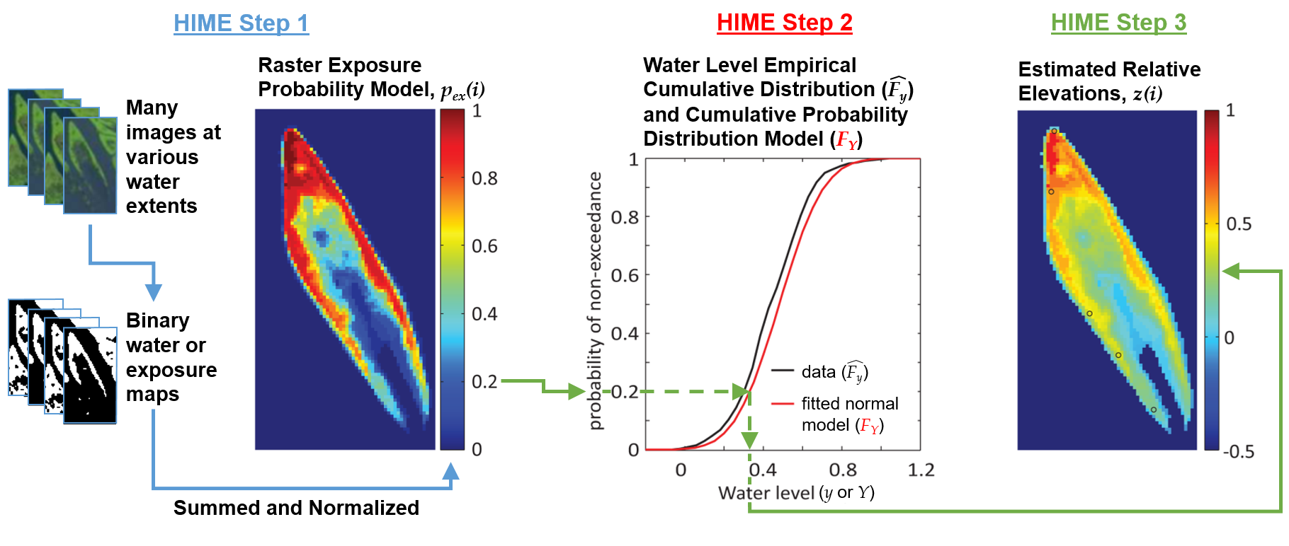
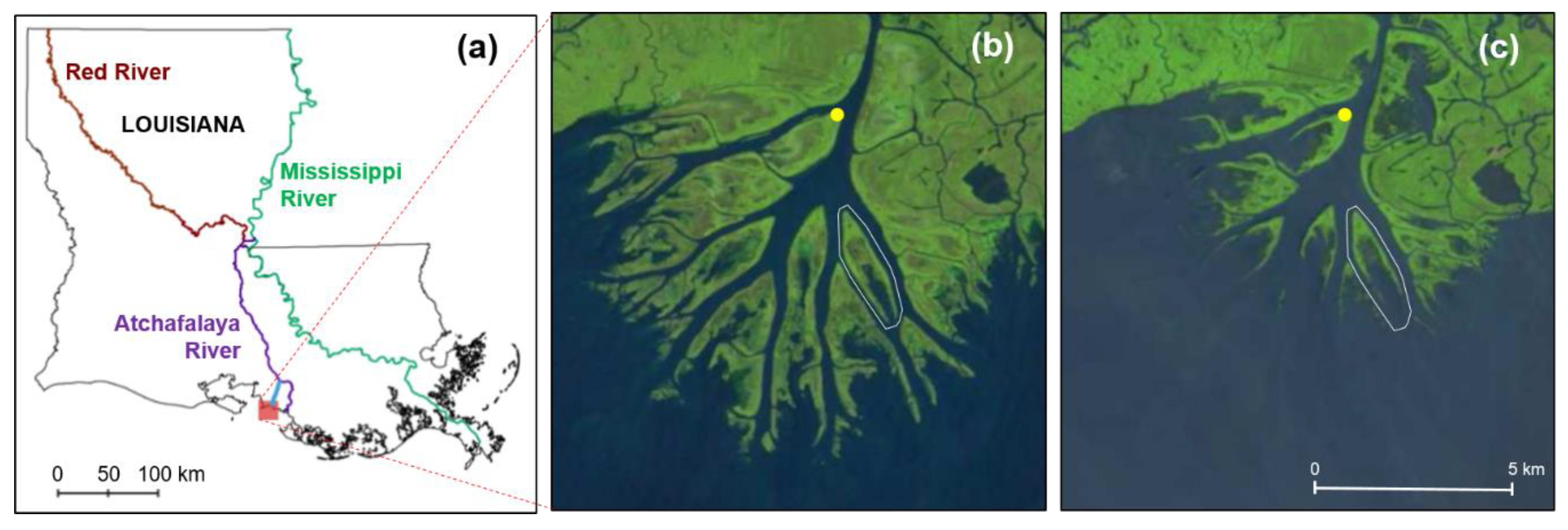
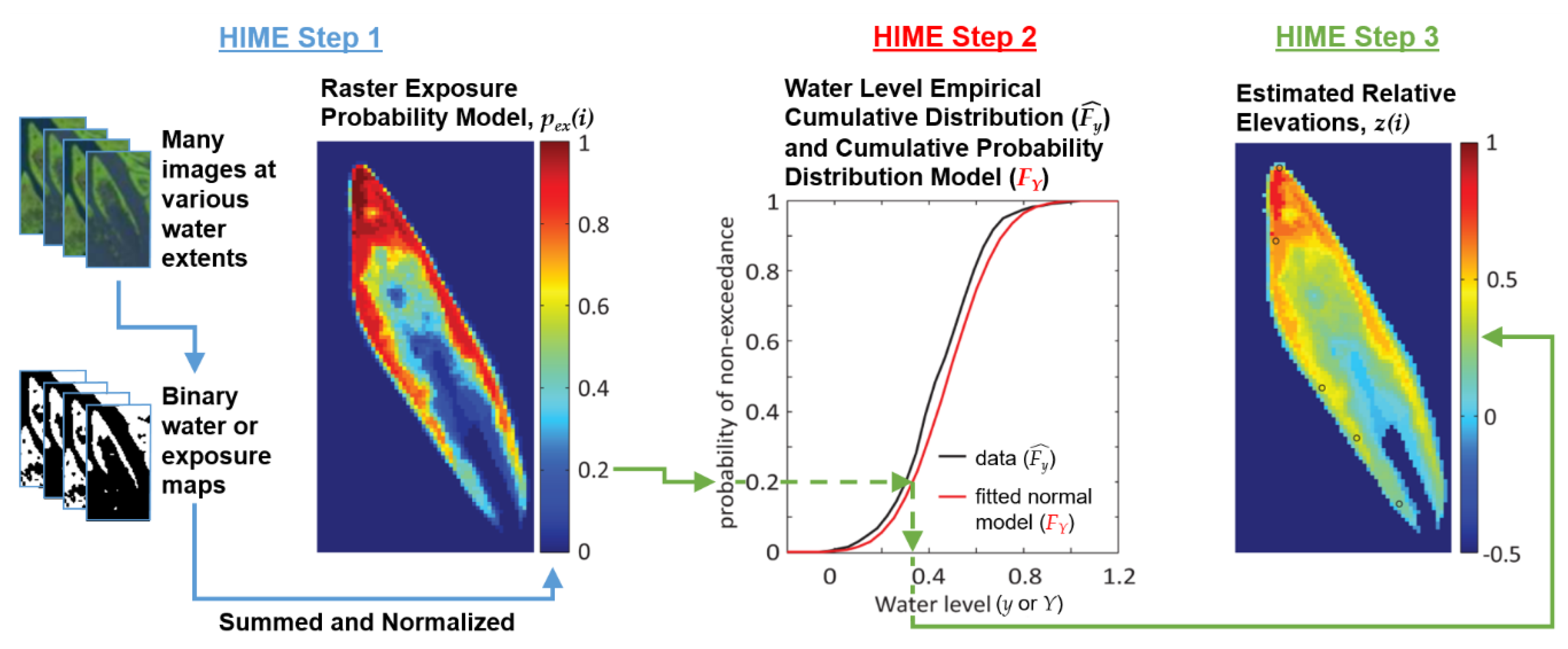
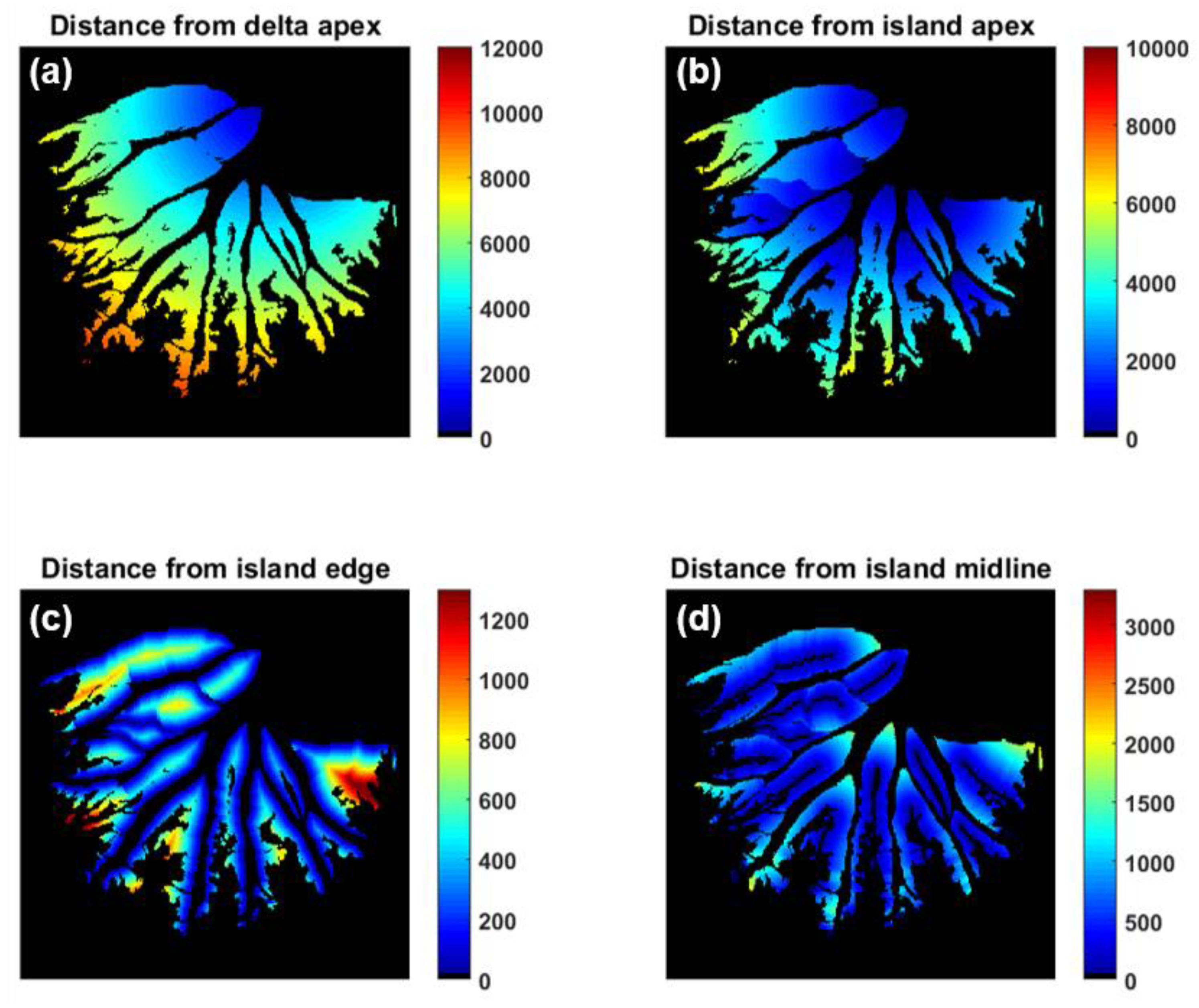
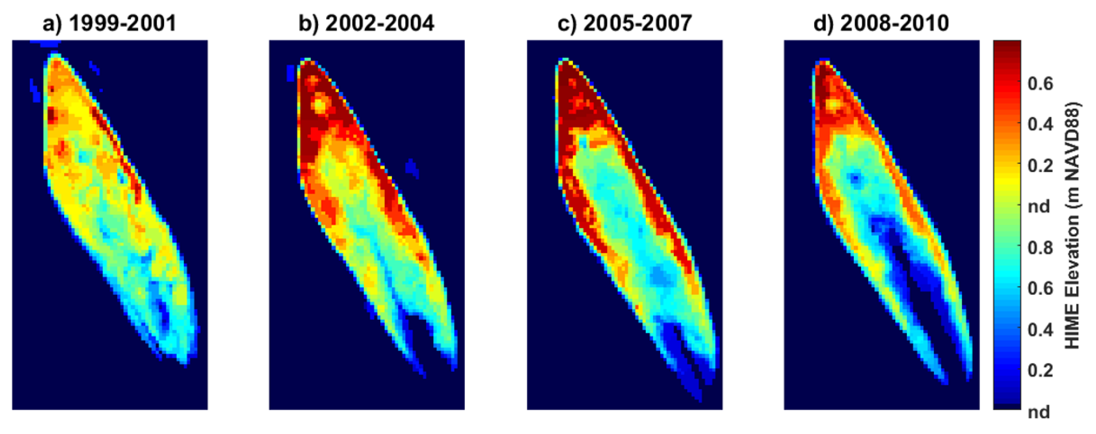
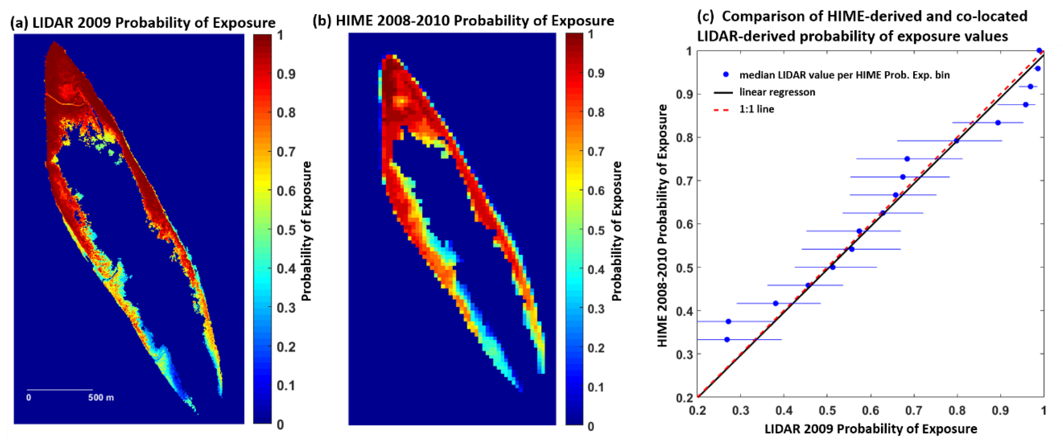
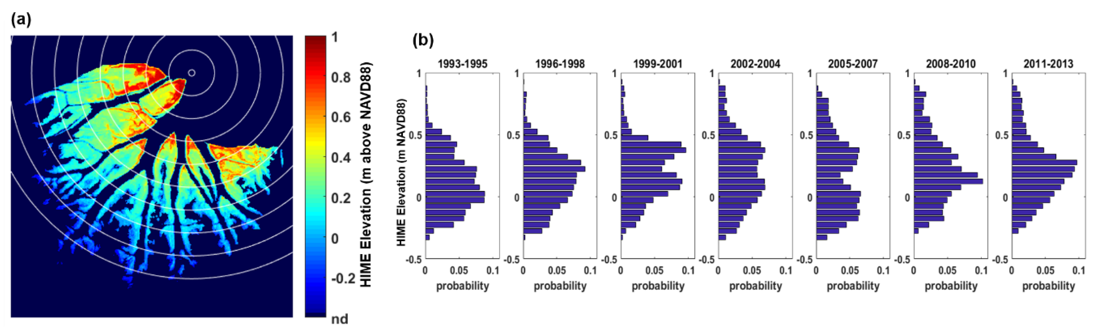
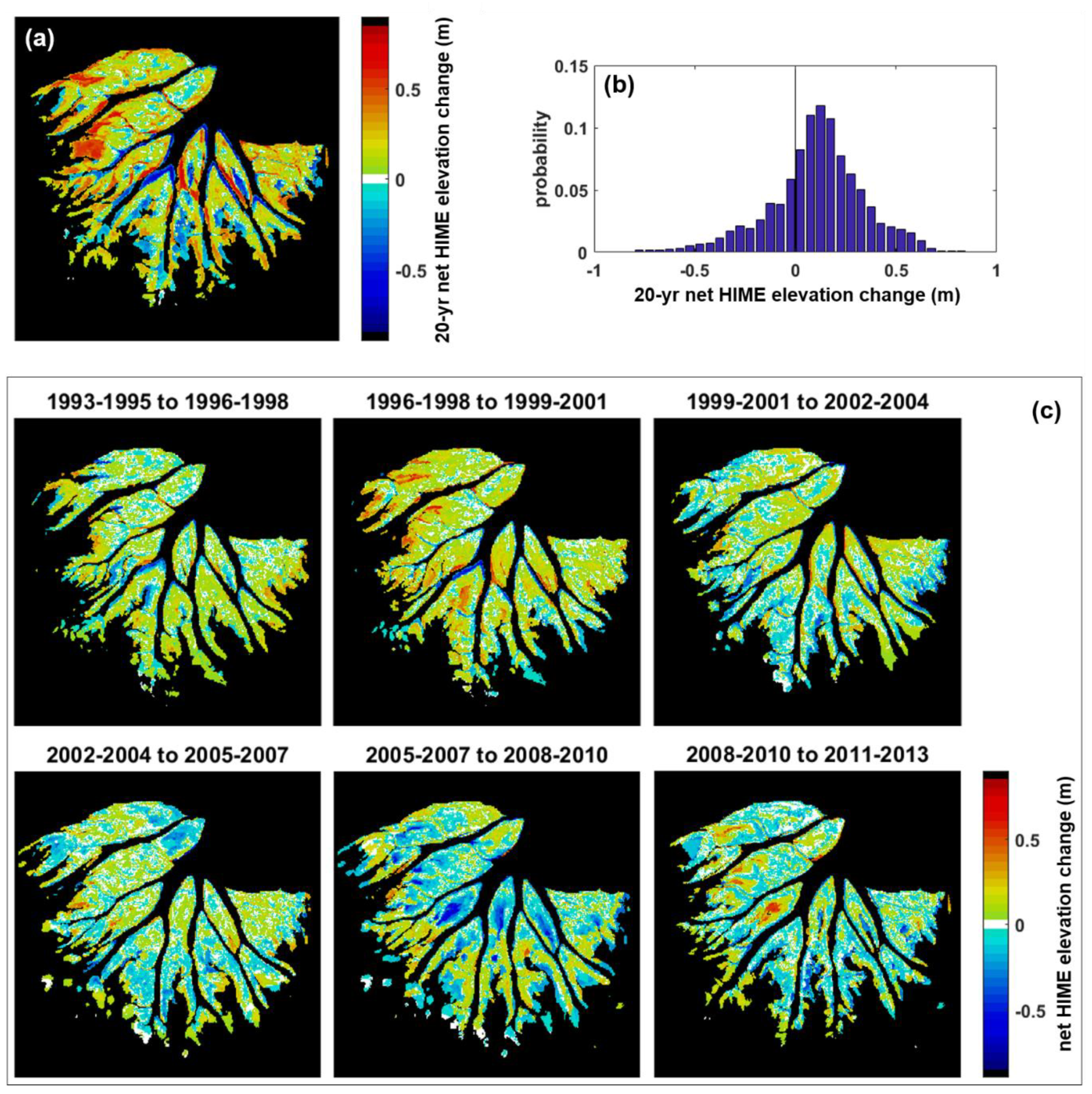
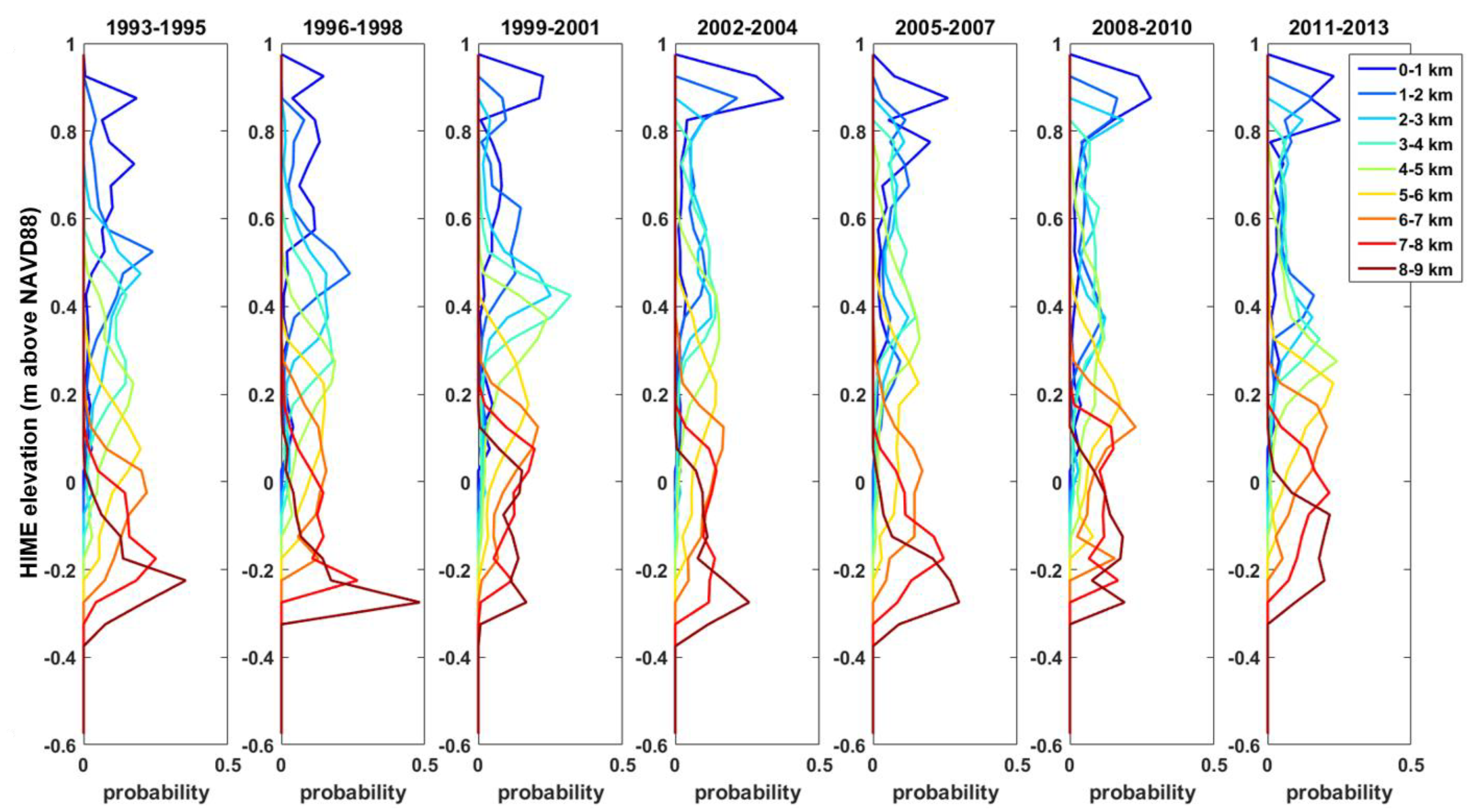
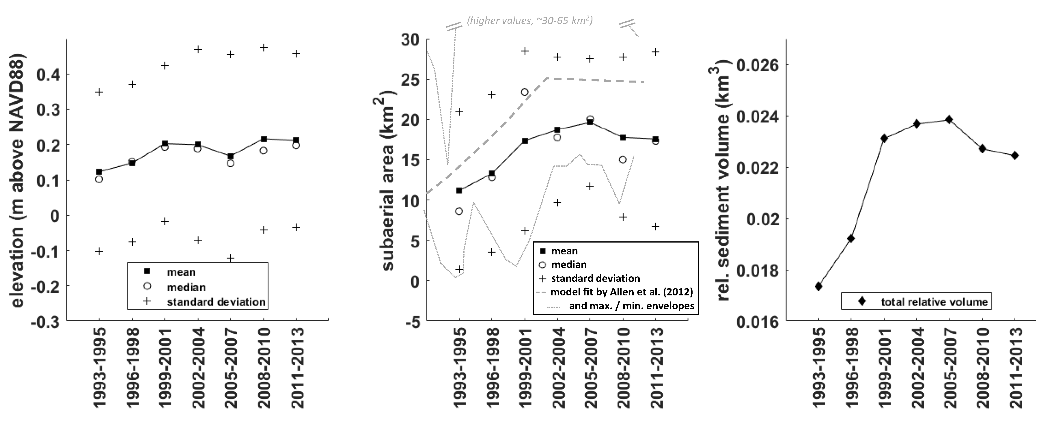
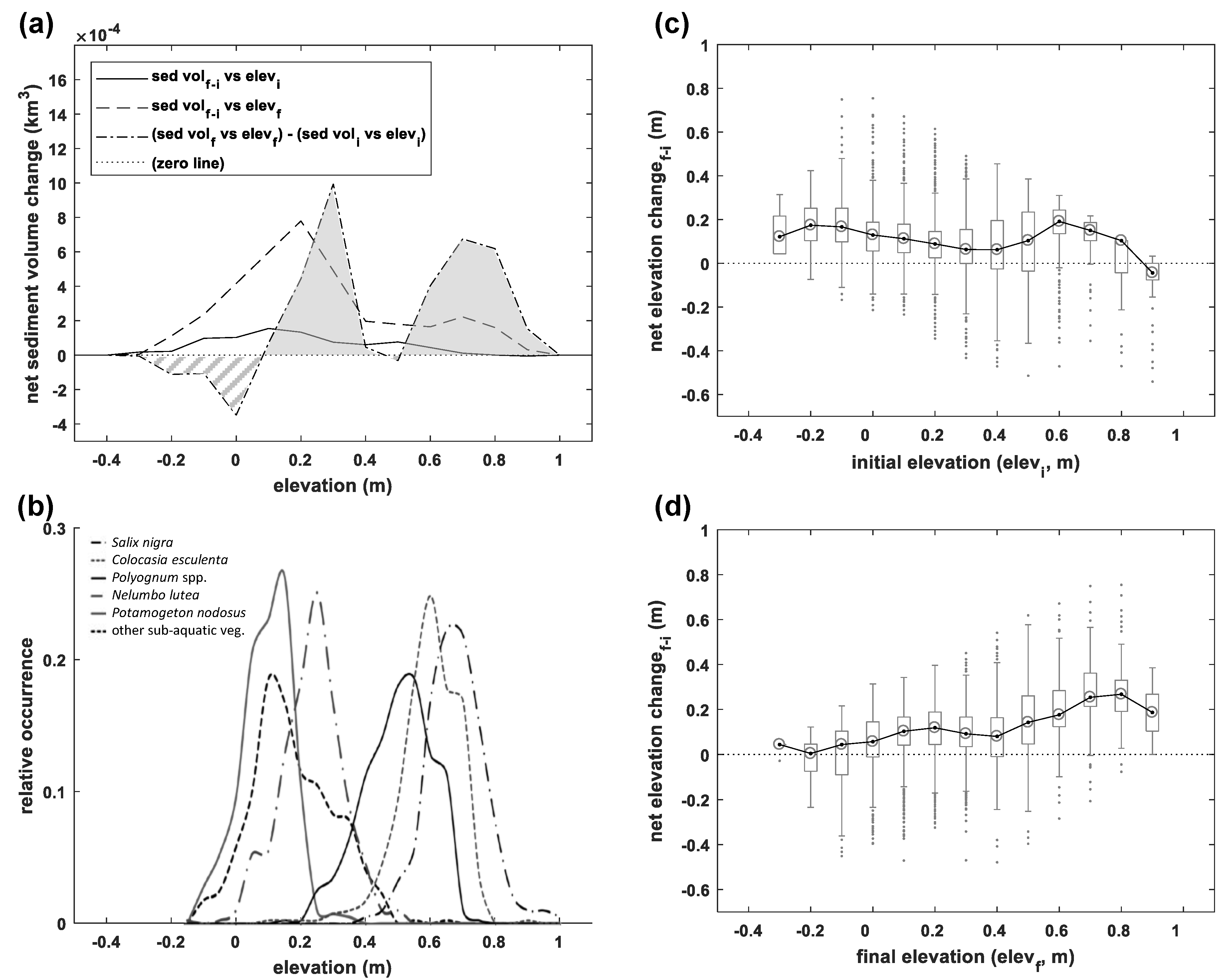
Table 1.
Linear regression model coefficients to predict elevation (m NAVD88) from geometric delta and island features (e.g., Figure 3), and median coefficients overall. Distances in km.
Table 1.
Linear regression model coefficients to predict elevation (m NAVD88) from geometric delta and island features (e.g., Figure 3), and median coefficients overall. Distances in km.
| Timeframe | Intercept | Dist. to Delta Apex (aj) | Dist. to Island Apex (bj) | Dist. to Channel Edge (cj) | Dist. to Island Midline (dj) | adj. R2 | RMSE |
|---|---|---|---|---|---|---|---|
| 1993–1995 | 0.6701 | −0.1007 | −0.0205 | −0.0108 | 0.0231 | 0.7343 | 0.1159 |
| 1996–1998 | 0.6833 | −0.0967 | −0.0175 | −0.0141 | 0.0213 | 0.7275 | 0.1169 |
| 1999–2001 | 0.7383 | −0.0962 | −0.0180 | 0.0053 | 0.0115 | 0.6841 | 0.1240 |
| 2002–2004 | 0.8833 | −0.1185 | −0.0247 | −0.0273 | 0.0232 | 0.7328 | 0.1398 |
| 2005–2007 | 0.8927 | −0.1184 | −0.0303 | −0.0201 | 0.0069 | 0.7380 | 0.1479 |
| 2008–2010 | 0.8093 | −0.1093 | −0.0206 | −0.0236 | 0.0664 | 0.6260 | 0.1580 |
| 2011–2013 | 0.7834 | −0.1062 | −0.0179 | 0.0066 | 0.0495 | 0.7014 | 0.1343 |
| median | 0.7834 | −0.1062 | −0.0205 | −0.0141 | 0.0231 | 0.7275 | 0.1343 |
Table 2.
Comparison of the multiple stable states of marsh elevations (stable platforms), vegetation, and water levels at the WLD by this study and others. Elevations in meters above NAVD88.
Table 2.
Comparison of the multiple stable states of marsh elevations (stable platforms), vegetation, and water levels at the WLD by this study and others. Elevations in meters above NAVD88.
| Reference | Evidence Source | Observ. Year (s) | Lowest Platform | Low Platform | Middle Platform | High Platform |
|---|---|---|---|---|---|---|
| Apparent Stable Elevations (Eco-geomorphic Attractors) | ||||||
| Smith et al. (2020) (this study) | HIME Landsat exposure probability; 3-year elevation histogram modes (Figure 6b) | 1999–2010 | 0.1 | 0.4 | 0.9 | |
| HIME elevation frequencies (Figure 8) | 1999–2013 | <0.5 | >0.7 | |||
| HIME most abundant final elevations (sed. volf−i vs elevf, Figure 10a) | 1993–2013 | 0.2 | 0.7 | |||
| HIME dz/dt ~ 0 (Figure 10c,d) | 1993–2013 | −0.3 | 0.4 | 0.9 | ||
| Olliver and Edmonds (2017) [27] | Intra-delta LIDAR analysis | 2012 | −0.12 | 0.25 | ||
| Wagner et al. (2017) [28] | Intra-delta and intra-annual LIDAR analysis | 2009, 2013 | 0.18 | 0.56 | ||
| O’Connor and Moffett (2015) [31] | field observation and sediment characteristics | 2013 | <0.45 | ≥0.45 | ||
| Ma, et al. (2018) [29] | Transfer entropy analysis and LIDAR change | 2009, 2013 | low | mid | high | |
| Twilley et al. (2019) [33] | <−0.04, below mean water | 0.04–0.30, intertidal | >0.30, supratidal | |||
| Apparent Focal Zones of Sedimentation (i.e., Elevation Change) or Biomass | ||||||
| Smith et al. (2020) (this study) | HIME net sediment volume change (sed. volf vs. elevf − sed. voli vs. elevi, Figure 10a) | 1993–2013 | Low loss: −0.3–0.05 | Low gain: 0.1–0.4 | High loss: 0.4–0.5 | High gain: 0.5–0.9 |
| Bevington and Twilley (2018) [30] | Soil organic matter (OM) content vs. elevation | 2010 | <0.0 * | 0.18–0.5 * | ||
| Carle et al. (2015) [32] | Marsh vegetation zones | 2010 | ~0.0–0.2 a | ~0.1–0.4 b | ~0.4–0.7 c | ~0.5–0.8 d |
* Bevington and Twilley (2018) noted sediment OM increase with elevation for marsh elevations >0.0 m NAVD88 [30]. We interpret, from their Figure 7 scatterplot, particular OM increase for marsh elevations >0.18 m, above which OM values were entirely >5% and increasing with elevation and below which OM values were almost entirely <5% with weaker elevation relationship. a Potamogeton nodosus, other submerged aquatic vegetation, b Nelumbo lutea, c Polyognum spp., and d Colocasia esculenta, Salix nigra vegetation zones, as by Carle et al. (2015) [32].
© 2020 by the authors. Licensee MDPI, Basel, Switzerland. This article is an open access article distributed under the terms and conditions of the Creative Commons Attribution (CC BY) license (http://creativecommons.org/licenses/by/4.0/).
Share and Cite
MDPI and ACS Style
Smith, B.C.; Moffett, K.B.; Mohrig, D. Short-Term Ecogeomorphic Evolution of a Fluvial Delta from Hindcasting Intertidal Marsh-Top Elevations (HIME). Remote Sens. 2020, 12, 1517. https://doi.org/10.3390/rs12091517
AMA Style
Smith BC, Moffett KB, Mohrig D. Short-Term Ecogeomorphic Evolution of a Fluvial Delta from Hindcasting Intertidal Marsh-Top Elevations (HIME). Remote Sensing. 2020; 12(9):1517. https://doi.org/10.3390/rs12091517
Chicago/Turabian StyleSmith, Brittany C., Kevan B. Moffett, and David Mohrig. 2020. "Short-Term Ecogeomorphic Evolution of a Fluvial Delta from Hindcasting Intertidal Marsh-Top Elevations (HIME)" Remote Sensing 12, no. 9: 1517. https://doi.org/10.3390/rs12091517
Note that from the first issue of 2016, this journal uses article numbers instead of page numbers. See further details here.