
Impact Assessment of Climate Change on Hailstorm Risk in Spanish Wine Grape Crop Insurance: Insights from Linear and Quantile Regressions

Department of Financial and Actuarial Economics & Statistics, Complutense University of Madrid, 28223 Pozuelo de Alarcón, Spain
*
Author to whom correspondence should be addressed.
†
These authors contributed equally to this work.
Risks 2024, 12(2), 20; https://doi.org/10.3390/risks12020020
Submission received: 30 December 2023
/
Revised: 19 January 2024
/
Accepted: 22 January 2024
/
Published: 26 January 2024
Abstract
:There is growing concern that climate change poses a serious threat to the sustainability of the insurance business. Understanding whether climate warming is a cause for an increase in claims and losses, and how this cause–effect relationship will develop in the future, are two significant open questions. In this article, we answer both questions by particularizing the geographical area of Spain, and a precise risk, hailstorm in crop insurance in the line of business of wine grapes. We quantify climate change using the Spanish Actuarial Climate Index (SACI). We utilize a database containing all the claims resulting from hail risk in Spain from 1990 to 2022. With homogenized data, we consider as dependent variables the monthly number of claims, the monthly number of loss costs equal to one, and the monthly total losses. The independent variable is the monthly Spanish Actuarial Climate Index (SACI). We attempt to explain the former through the latter using regression and quantile regression models. Our main finding is that climate change, as measured by the SACI, explains these three dependent variables. We also provide an estimate of the increase in the monthly total losses’ Value at Risk, corresponding to a future increase in climate change measured in units of the SACI. Spanish crop insurance managers should carefully consider these conclusions in their decision-making process to ensure the sustainability of this line of business in the future.
1. Introduction
According to the United Nations Climate Action Forum, “climate change refers to long-term shifts in temperatures and weather patterns. Such shifts can be natural, due to changes in the sun’s activity or large volcanic eruptions. But since the 1800s, human activities have been the main driver of climate change, primarily due to the burning of fossil fuels like coal, oil and gas. Burning fossil fuels generates greenhouse gas emissions that act like a blanket wrapped around the Earth, trapping the sun’s heat and raising temperatures” UN (2023). This process is a long-term one, affecting human beings in many ways, such as their lives, properties, transportation infrastructures, etc. (see, for instance, Pryor 2017; Warren-Myers et al. 2018; Dundon et al. (2016)). As the insurance business permeates all aspects of economic and individual human life, providing protection against various claims and substituting random losses with assured indemnities, the question of how climate change is affecting the insurance business has emerged as a critical concern for its present management and future sustainability.
In recent years, numerous extreme events, such as fires, floods, droughts, storms, and pandemics, have adversely impacted the balance sheets of insurance companies, prompting them to withdraw from certain lines of business in geographical areas where losses have surged to unaffordable levels (see, for instance, AP 2023). In the scientific world, the concern for the sustainability of the insurance business has led to numerous efforts to understand how insurance companies should incorporate the effects of climate change into their medium- and long-term management (see Wagner 2022; Rao and Li 2023; Courbage and Golnaraghi 2022; Thistlethwaite and Wood 2018; Savitz and Dan Gavriletea 2019). The efforts to technically cope with the new situation involve the application of advanced statistical and data science methodologies (see, for instance, Li and Tang 2022; Lyubchich et al. 2019; Miljkovic et al. 2018; Heranval et al. 2022). General insurance principles such as risk insurability, pooling, and diversification are also under discussion in the context of climate shift (Charpentier 2008). The insurance areas analyzed from the perspective of climate change include those related to mortality and property losses (see, for instance, Li and Tang 2022; Miljkovic et al. 2018). Another significant field of research is agricultural insurance (Al-Maruf et al. 2021; Jørgensen et al. 2020), which is the focus of our paper. In crop insurance, all weather-related extreme events are relevant and may be influenced by climate change.
This paper focuses on hailstorm risk in the Spanish crop insurance line of business of wine grapes. This poses a daunting challenge for insurance managers due to its variability in both time and space and the fact that its occurrences are relatively local and ubiquitous. Hail risk in agricultural insurance has been analyzed in previous studies, such as Portmann et al. (2023), Simbürger et al. (2022), and Reyes et al. (2020). While hailstorms can be highly damaging to crops, their evolution under global warming has seldom been studied. In Raupach et al. (2021), the authors explore the influence of conditions such as moisture and convective instability on the generation of hailstones, providing a geographical outlook on the future frequency evolution of hailstorms. Notably, it suggests a potential increase in Europe as anthropogenic warming continues. Another study, Botzen et al. (2010), employs Tobit regressions and finds a strong positive relationship between hailstorm activity and damage, correlated with minimum temperatures. This relationship implies that hailstorm damage may escalate in the future if global warming leads to further temperature increases. Finally, Niall and Walsh (2005) observe a significant influence of climate change, measured by Convective Available Potential Energy (CAPE) and the totals–totals index (TT index), on the frequency and intensity of hail events in various locations around southeastern Australia. The study utilizes reanalysis data (a dataset comprising a blend of observations and model simulations) and direct data obtained from the Australian National Climate Centre.
In this research, we employ successive regression and quantile regression models to investigate whether climate change influences hailstorm risk at both the expectation and high quantile levels of certain insurance-relevant variables, such as the monthly number of claims, loss costs equal to one, and total losses. Regression is a crucial methodology in insurance rate making (see, for instance, Lemaire 2012; Denuit et al. 2007; De Jong and Heller 2008; and Vilar-Zanón et al. 2020 for posterior rate making in agricultural insurance). Quantile regression is a non-parametric methodology that extends the idea of regression to quantiles and traces back to Koenker and Bassett (1978). We will apply it using the R package quantreg (Koenker 2015). This methodology is more recent in its application to insurance and is basically oriented to rate making; see, for instance, Heras et al. (2018) and Baione and Biancalana (2018).
The cultivation of Spanish wine grapes constitutes a particularly significant segment in agricultural insurance, especially considering that Spain boasts the largest cultivated area for wine grapes among all of the European countries (Statista 2023). Based on our model results, we conclude that climate change accounts for the observed increase in the related variables from 1990 to 2022.
2. Materials and Methods
2.1. The Database on Hail Risk in Spanish Wine Grapes
The database on wine grape hailstorm claims is sourced from Agroseguro, the Spanish coinsurance pool of agricultural insurance, grouping seventeen insurance companies. Agroseguro manages the risks and policies on behalf of those companies and participates in the Spanish system of agricultural insurance, together with the Spanish State and professional agricultural associations and cooperatives. During the year 2022, its wine grapes line of business has insured 46.44% of the total 860,791 ha of cultivated surface, and the total value of the production (total insured sum) has been EUR 1091.28 M (see Agroseguro 2023).
The database comprises 7,547,286 records spanning from 1990 to 2022, containing information on 49 provinces and 240 regions, with 893,144 yearly policies. Over the 33 years, there have been 692,733 claims, and relevant yearly figures are presented in Table 1. Figure 1 visually depicts the evolution of both the number of plots and hailstorm claims during the specified period. Consequently, this comprehensive database offers a detailed perspective on hailstorm risk in the Spanish wine grapes line of business from 1990 to 2022. The ’Crop Yield’ column in Table 1 is derived from individual plot information within the database, representing the expected potential production in each insured plot based on its normal edaphic, climatic, planting, sowing, and cultivation conditions.
The claim data have been aggregated monthly, and months without claims have been filled with zeros, as shown in the blank spaces in Table 2. This approach enables a nuanced understanding of seasonal patterns and trends over the years. Such detail is crucial for studying the impact of climate change, particularly in determining the relevant season for hailstorms, which will be later defined as a sequence of months.

Table 1.
Spanish wine grape insurance data, yearly figures.
| Year | Total Insured Sum (EUR) | Total Loss (EUR) | Crop Yield (kg) | Number of Policies | Number of Plots | Number of Claims |
|---|---|---|---|---|---|---|
| 1990 | 217,652,835 | 6,200,518 | 1,388,430,463 | 28,100 | 134,050 | 15,291 |
| 1991 | 248,557,853 | 3,560,276 | 1,550,473,335 | 31,621 | 152,005 | 12,000 |
| 1992 | 307,714,572 | 7,904,540 | 1,912,566,029 | 39,929 | 198,611 | 19,235 |
| 1993 | 284,919,972 | 6,826,730 | 1,829,365,370 | 37,832 | 195,007 | 17,456 |
| 1994 | 297,271,994 | 2,738,423 | 1,901,295,250 | 38,984 | 204,313 | 8619 |
| 1995 | 242,077,610 | 5,569,047 | 1,400,284,025 | 29,129 | 167,305 | 18,063 |
| 1996 | 327,901,655 | 4,593,910 | 1,605,894,257 | 32,859 | 193,004 | 9282 |
| 1997 | 395,633,563 | 14,096,834 | 1,957,379,446 | 37,049 | 225,642 | 25,611 |
| 1998 | 441,049,489 | 13,007,045 | 1,971,311,184 | 34,288 | 213,158 | 17,656 |
| 1999 | 437,265,055 | 14,794,992 | 1,917,674,498 | 32,706 | 206,014 | 24,029 |
| 2000 | 568,328,639 | 9,741,835 | 2,090,534,475 | 34,000 | 219,489 | 10,682 |
| 2001 | 560,603,175 | 6,759,693 | 2,011,166,692 | 30,996 | 201,894 | 7641 |
| 2002 | 522,149,823 | 7,945,331 | 1,943,561,894 | 28,876 | 190,731 | 13,152 |
| 2003 | 562,951,706 | 18,847,196 | 2,076,438,149 | 29,037 | 195,308 | 16,855 |
| 2004 | 598,344,779 | 18,271,523 | 2,163,019,536 | 28,823 | 199,977 | 17,954 |
| 2005 | 595,592,273 | 10,960,930 | 2,098,146,664 | 26,412 | 198,760 | 14,503 |
| 2006 | 551,669,449 | 23,246,532 | 1,899,984,824 | 23,194 | 183,900 | 22,537 |
| 2007 | 577,020,427 | 42,553,289 | 1,964,259,110 | 22,665 | 189,357 | 22,043 |
| 2008 | 653,256,796 | 15,265,573 | 2,230,822,485 | 24,461 | 210,449 | 14,725 |
| 2009 | 628,159,377 | 19,773,933 | 2,097,168,866 | 21,950 | 204,072 | 14,280 |
| 2010 | 597,317,970 | 10,530,360 | 1,951,036,257 | 19,993 | 193,284 | 13,732 |
| 2011 | 516,300,441 | 23,659,028 | 1,746,476,820 | 17,927 | 174,013 | 21,883 |
| 2012 | 644,892,414 | 15,259,638 | 2,292,548,909 | 21,480 | 209,162 | 11,043 |
| 2013 | 630,157,964 | 30,235,918 | 2,268,987,633 | 21,075 | 231,153 | 32,294 |
| 2014 | 687,759,537 | 18,986,141 | 2,389,698,870 | 20,650 | 238,865 | 26,823 |
| 2015 | 704,818,295 | 33,449,574 | 2,426,866,357 | 20,139 | 243,458 | 37,138 |
| 2016 | 772,792,789 | 11,049,778 | 2,633,586,202 | 20,947 | 268,232 | 11,205 |
| 2017 | 821,585,396 | 20,152,939 | 2,768,418,806 | 21,023 | 284,922 | 25,283 |
| 2018 | 939,523,058 | 37,068,415 | 3,010,843,844 | 22,839 | 333,156 | 39,809 |
| 2019 | 1,028,808,795 | 29,643,282 | 3,154,082,113 | 23,467 | 359,053 | 34,916 |
| 2020 | 1,038,651,982 | 41,498,451 | 3,159,232,107 | 23,636 | 368,346 | 40,465 |
| 2021 | 1,056,633,225 | 53,137,810 | 3,192,077,192 | 23,537 | 372,611 | 48,217 |
| 2022 | 1,091,289,076 | 30,551,509 | 3,279,107,478 | 23,520 | 387,991 | 28,479 |
Figure 1.
Yearly numbers of plots (blue) and claims (pink) over the time period.

Table 2.
The normalized monthly number of claims.
| Jan | Feb | Mar | Apr | May | Jun | Jul | Aug | Sep | Oct | Nov | Dec | |
|---|---|---|---|---|---|---|---|---|---|---|---|---|
| 1990 | 0.0015 | 0.3081 | 2.3514 | 0.4118 | 1.5308 | 3.1197 | 3.6792 | |||||
| 1991 | 0.0408 | 0.4092 | 0.1895 | 2.2058 | 0.3756 | 4.6512 | 0.0164 | 0.0007 | ||||
| 1992 | 0.0030 | 1.6162 | 1.2416 | 2.4082 | 3.4349 | 0.9415 | 0.0227 | |||||
| 1993 | 0.0021 | 0.3123 | 1.3200 | 2.8835 | 1.5353 | 1.9061 | 0.9230 | 0.0692 | ||||
| 1994 | 0.0015 | 0.4033 | 1.0053 | 1.2045 | 0.3132 | 0.9862 | 0.2966 | 0.0078 | ||||
| 1995 | 0.0048 | 0.7208 | 1.0663 | 1.0185 | 0.9091 | 5.9801 | 1.0831 | 0.0030 | ||||
| 1996 | 0.0047 | 0.3280 | 0.4000 | 0.9746 | 1.4430 | 1.0098 | 0.6124 | 0.0326 | ||||
| 1997 | 0.0004 | 0.0049 | 0.0315 | 1.3145 | 0.6107 | 3.8978 | 4.5687 | 0.9161 | 0.0031 | |||
| 1998 | 0.0033 | 0.0009 | 0.0033 | 1.6504 | 1.3586 | 2.4189 | 0.4372 | 1.9502 | 0.4199 | 0.0403 | ||
| 1999 | 0.0005 | 0.0010 | 0.2451 | 0.9053 | 2.4848 | 3.5968 | 0.4713 | 3.9575 | ||||
| 2000 | 0.0023 | 0.0838 | 1.5768 | 0.8388 | 0.5627 | 1.0215 | 0.7795 | |||||
| 2001 | 0.0490 | 1.2437 | 0.0064 | 0.9000 | 0.6142 | 0.8524 | 0.1184 | |||||
| 2002 | 0.0005 | 0.0661 | 0.2144 | 0.6218 | 1.0785 | 3.7844 | 1.0963 | 0.0131 | ||||
| 2003 | 0.0005 | 0.0046 | 0.5765 | 2.2529 | 0.9503 | 3.6619 | 1.1833 | |||||
| 2004 | 0.0020 | 0.1340 | 0.5636 | 1.4272 | 1.8632 | 1.7572 | 3.1424 | 0.0835 | ||||
| 2005 | 0.0010 | 0.0795 | 0.4593 | 2.3747 | 2.2228 | 1.3232 | 0.8226 | 0.0136 | ||||
| 2006 | 1.0962 | 0.5753 | 4.6688 | 4.4209 | 1.0120 | 0.4818 | ||||||
| 2007 | 0.0037 | 1.1259 | 8.2833 | 0.9670 | 0.0438 | 0.7763 | 0.4309 | 0.0048 | ||||
| 2008 | 0.0048 | 0.0889 | 2.6448 | 0.7579 | 1.5101 | 0.6781 | 1.2972 | 0.0048 | 0.0010 | |||
| 2009 | 0.0304 | 2.0101 | 1.7969 | 0.6243 | 2.0924 | 0.4425 | 0.0010 | |||||
| 2010 | 0.0005 | 0.0021 | 0.5143 | 1.8755 | 1.2003 | 1.8227 | 1.3855 | 0.3032 | ||||
| 2011 | 0.0086 | 1.0183 | 6.0122 | 1.5964 | 1.8861 | 1.9119 | 0.1419 | |||||
| 2012 | 0.0010 | 0.4174 | 2.0032 | 0.6574 | 1.7685 | 0.3151 | 0.1143 | 0.0029 | ||||
| 2013 | 0.0017 | 0.0346 | 4.3339 | 0.7419 | 4.9547 | 1.7841 | 1.3454 | 0.7735 | ||||
| 2014 | 0.0599 | 0.6962 | 3.8486 | 4.4770 | 0.8302 | 1.3162 | 0.0013 | |||||
| 2015 | 0.0008 | 0.2234 | 2.6530 | 2.7483 | 4.9491 | 3.2531 | 1.4265 | |||||
| 2016 | 0.0112 | 0.1831 | 1.0293 | 0.4351 | 1.0908 | 0.2427 | 1.1151 | 0.0701 | ||||
| 2017 | 0.8560 | 1.1796 | 3.4915 | 2.5200 | 0.5728 | 0.2538 | ||||||
| 2018 | 0.0018 | 0.3554 | 1.8739 | 1.9648 | 4.4922 | 2.0924 | 1.1679 | 0.0006 | ||||
| 2019 | 0.0042 | 0.3228 | 0.9428 | 0.0089 | 4.6236 | 2.9622 | 0.8600 | |||||
| 2020 | 0.0176 | 0.6532 | 0.9893 | 2.9904 | 3.8605 | 2.2446 | 0.2259 | 0.0041 | ||||
| 2021 | 0.3387 | 0.7536 | 5.1348 | 0.6975 | 2.4414 | 3.5740 | 0.0003 | |||||
| 2022 | 0.0034 | 0.1925 | 0.5289 | 0.1497 | 2.3617 | 3.7429 | 0.3593 | 0.0018 |
2.1.1. The Normalized Number of Claims, N
We normalize the number of claims (yearly or monthly) by dividing it by the number of plots for that year. In essence, we calculate the proportion of policies on which claims occurred compared to the total number of plots for that year (refer to Table 2 for monthly figures).
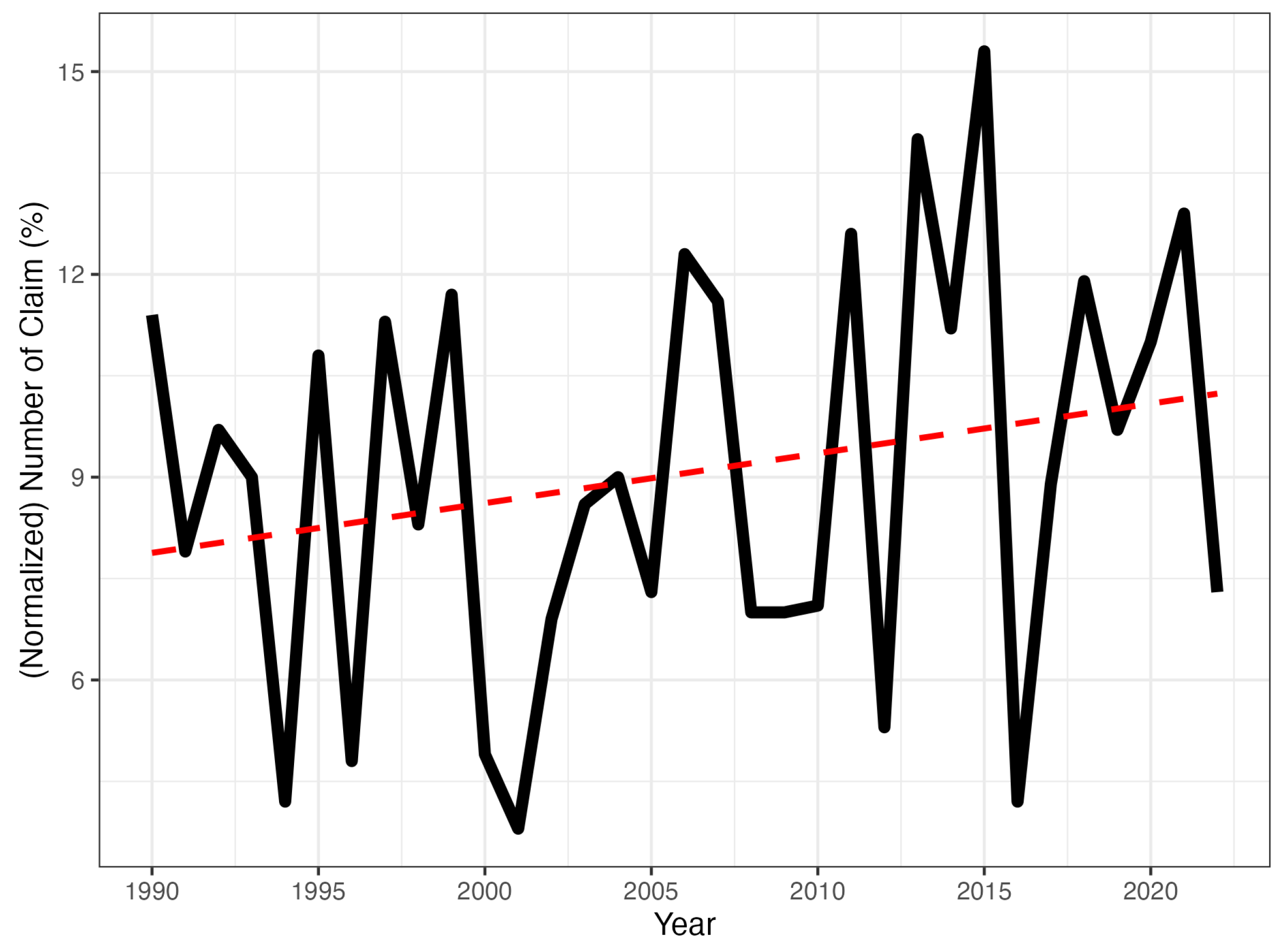
The plot of normalized yearly claims is illustrated in Figure 2. It showcases the actual yearly trend in the number of hailstorm claims in the Spanish wine grape line of business from 1990 to 2022, considering the growth in the number of plots. The graph reveals a jagged shape, indicating significant variation in the yearly number of claims, reflecting the high uncertainty and variability of hailstorm risk. Nevertheless, its upward trend suggests an increase in the frequency of the normalized number of hailstorm events, a phenomenon we aim to explain through climate warming.
Figure 3 illustrates the trend in the number of monthly hailstorm claims from January 1990 to December 2022. The data are normalized to more accurately depict the relative changes in the number of claims from month to month.
Additionally, in Table 2 and Figure 3, we observe a significant and clear seasonal pattern. The majority of hail claims occur from April to September, a pattern likely associated with the weather conditions that lead to hailstorms and the growth cycle of wine grapes. This observation is crucial as it allows us to define the period from April to September as the hailstorm season, which will be utilized in our models to explain insurance claims and losses attributed to climate change.
2.1.2. The Normalized Number of Loss Costs Equal to One,
The loss cost is determined by the ratio of severity over insured capital, offering a straightforward measure of the extent of damage caused by a claim. Moving forward, we will denote for the monthly number of loss costs equal to one (the time-frame, whether monthly or yearly, will be evident from the context). When , it signifies that the number of losses equals the insured capitals, indicating the maximum level of burden for the insurance company in those claims. In Figure 4, we present the yearly normalized as a percentage of the yearly number of claims. While the rate remains low in most years, several spikes indicate instances where hailstorms resulted in significant economic losses. The least squares line, overall, demonstrates an increasing trend, suggesting a rise in the maximum damages over time. Our goal is to elucidate this long-term increase through the influence of climate change.
2.1.3. The Homogenized Losses, L
Over time, factors such as inflation, increases in the number of policies and/or cultivated surfaces, and rising productivity levels may influence insurance losses. Consequently, claims of similar intensity at different dates may lead to larger losses than in previous years. Therefore, implementing a homogenization process becomes crucial when analyzing insurance losses over time. This homogenization enables more accurate and fair comparisons across time, facilitating a thorough understanding of the changing impacts of insurance claims and their economic consequences (see Botzen et al. 2010; Pielke and Landsea 1998; Barthel and Neumayer 2012).
In our research, we use a specific normalization formula to analyze hailstorm losses. This formula allows us to effectively compare loss data across different years, even in changing market conditions and agricultural productivity. The formula for normalized insurance loss is:
where represents the total insurance losses, where , and . The is a specially designed index that accounts for annual changes in insurance capital and crop yields since 1990. The calculation method for the insurance value index is as follows:
This index is an annual time series that comprehensively accounts for changes in total insurance capital and crop yields since 1990. Specifically, the index reflects the relative changes in annual insurance capital compared to the baseline level in 1990. It also incorporates yearly variations in crop yield to reflect fluctuations in agricultural production and market conditions. Through this approach, our insurance value index effectively homogenizes hailstorm loss data across different years, enabling fair and consistent comparisons. Thus, even amid changes in market conditions and agricultural productivity, we can accurately measure and analyze the trends and impacts of hailstorm losses. Henceforth, we will consistently work with homogenized losses, even when briefly referred to as losses.
The consideration of the logarithm of insurance losses is motivated by two key factors. Firstly, this transformation helps moderate the impact of outliers on the model by reducing data dispersion, contributing to a more robust model. Secondly, the logarithmic transformation stabilizes the variance structure of the data, enhancing the accuracy of the regression (see Benoit 2011). As depicted in Figure 5, logarithmic losses exhibit greater stability than the original ones. Notably, we apply the logarithmic transformation only to months with claims, while months with no claims are recorded as zeroes.
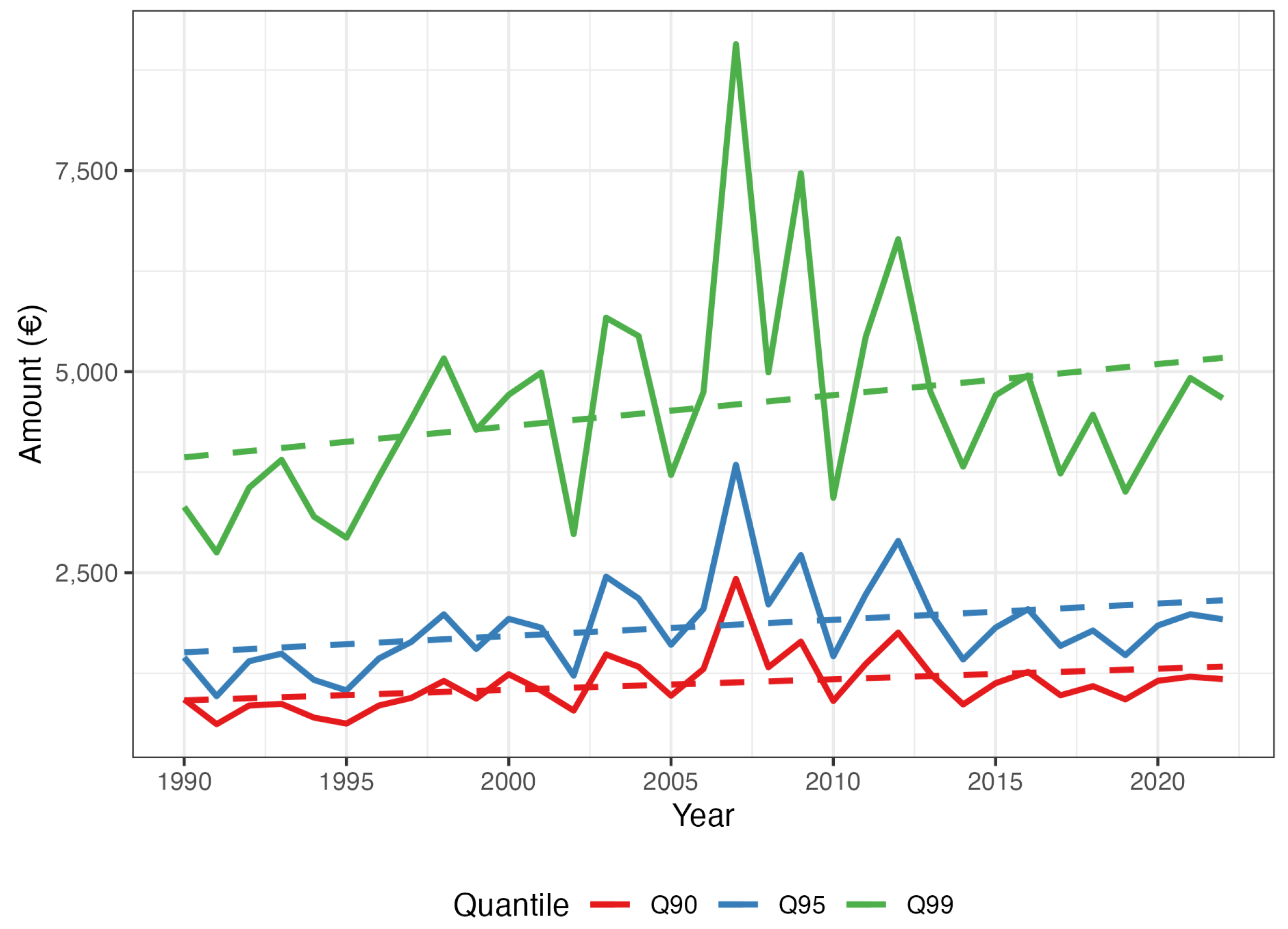
We can further analyze the total loss variable by examining its yearly figures in Figure 6, where three of its yearly quantiles (90th, 95th, and 99th) are plotted, revealing increasing trends over time in all three cases. This growth seems to support the idea that climate-change influence might still be significant for higher probability levels, not only for means. We aim to test this hypothesis later. Finally, it is worth noting that if the frequency and severity of hailstorm extreme events continue to increase over time, this could potentially impact the business’s sustainability. To what extent, though? We attempt to quantify this effect in our later analysis.
2.2. The Spanish Actuarial Climate Index (SACI)
Up to this point, we have presented and explained the data related to the dependent variables: the normalized monthly number of claims (N), the normalized number of loss costs equal to one (), and the homogenized monthly total losses (L). We now shift our focus to the independent variable, where our aim is to use an index of climate change.
To assist insurance companies in measuring and managing climate risk, actuaries in North America have defined the Actuaries Climate Index™ (ACI). This index combines information from several crucial weather variables derived from the historical records of the United States and Canada. The ACI divides the main geographical area (USA and Canada) into a grid of cells corresponding to a specific resolution. It then collects relevant historical meteorological data for each cell to calculate the six ACI components: days of warm temperature (), days of cool temperature (), precipitation (P), drought (D), wind speed (W), and sea level (S). For each cell, the ACI utilizes the reference period from 1961 to 1990. Mean and standard deviations are calculated for all the components during this period. Subsequently, the data are normalized by these figures, allowing variations to be measured in units of the corresponding reference period standard deviation. Subsequently, the ACI calculates the mean of the six normalized components to derive a cell-wise index. Notably, the T10 component is subtracted to ensure a meaningful magnitude:
Finally, the ACI relative to any geographical area within the main one is calculated as the average of the cell-wise indexes covering the area of interest. Additionally, the ACI can be customized for any given season by collecting the data specific to that season and following the same process. In summary, any increase in ACI observed after 1990 will indicate a warming trend in that area, approximately measured in standard deviation units (see ACI 2018).
The Iberian Actuarial Climate Index (IACI) is the specific actuarial climate index for the Iberian Peninsula, constructed using the ACI method (see Zhou et al. 2023), but utilizing data specific to the Iberian Peninsula sourced from the ERA5 Re-Analysis. The ERA5-Land reanalysis data is a high-resolution dataset with a horizontal resolution of 0.1° × 0.1° for each grid cell, generated by replaying the land component of the ECMWF ERA5 climate reanalysis. Reanalysis combines model data with observations from various sources, including satellites, weather stations, and ocean buoys (see Zhou et al. 2023). For our analysis, we will leverage the Spanish regional monthly index derived from the Iberian Actuarial Climatic Index (SACI), providing a comprehensive understanding of climatic changes in Spain.
Figure 7 illustrates the variation in the SACI from April to September for each year spanning from 1961 to 2022. Examining these subplots reveals noticeable trends, particularly in certain months such as July and August, which exhibit a significant upward trend in recent years. Conversely, other months, such as April and May, display relatively stable fluctuations. The graph unveils changes in climatic conditions during the peak season of hail disasters each year. Importantly, the rising trend observed from April to September may indicate alterations in meteorological conditions within these months, potentially linked to broader trends in global climate change.
2.3. Methods: Linear and Quantile Regressions
This paper aims to investigate the relationship between the Spanish Actuarial Climate Index (SACI) and its components and hailstorm damages in the Spanish wine grapes insurance line of business. We utilize both linear regression models (Weisberg 2005) and quantile regression methods (Koenker 2005) to analyze the data. Linear regression is a commonly employed technique for estimating the linear association between a dependent variable and one or more independent variables. Its general formula is expressed as follows:
In (4), Y represents the dependent variable, are the independent variables, is the intercept, are the coefficients, and is the error term. For the sake of concision, linear models such as (4) will be noted as:
For quantile regression, the general form is:
where denotes the quantile of the conditional distribution of the response variable Y given the design matrix X with columns , and the vector represents the quantile regression coefficients. Again for the sake of concision, a model such as (6) will be noted as:
Linear regression offers insights into the relationship between the SACI and the expectations of hailstorm claims variables, whereas quantile regression provides similar insights for their quantiles.
As mentioned earlier, hailstorm claims for Spanish wine grapes are predominantly reported from April to September, corresponding to the primary occurrence of hail claims. In the subsequent analysis, three independent variables related to hail claims will be utilized:
- Monthly normalized number of claims, N.
- Monthly number of loss costs equal to one, .
- Monthly homogenized total losses, L.
In linear regression, can be calculated as:
where is the sum of squares of residuals and is the total sum of squares. In quantile regression, we will calculate a pseudo- for the goodness of fit that is no longer based on Ordinary Least Squares (OLS) calculations but on absolute errors (see Koenker and Machado 1999), using the R function goodfit().
3. Results
3.1. Monthly Normalized Number of Claims, N
In Table 3, we present the results of three linear regression models designed to explore the relationship between climate variables, such as the SACI and its components, and the mean of N.
In model 1
we explore the influence of the monthly SACI on the mean of N and find it to be significant at a level. This suggests a certain influence on the number of hail claims. However, the deficient indicates that the SACI alone does not explain the variations well in the mean of N.
In model 2,
we introduce the components of the SACI to discern their impact on the mean of N. Notably, high-temperature days () and sea level () are significant, suggesting a potential link between these two SACI components and the mean. However, despite their significance, the overall explanatory power of the model, as indicated by , remains low. While extreme heat and sea level contribute to the predictive model, additional variables are needed to enhance the accuracy of the analysis.
In model 3, we test the formula
which incorporates the months from April to September, covering the high-incidence season of hailstorms. Despite the statistical significance observed for precipitation () and wind () with coefficients of opposite signs, the overall explanatory power of the model, indicated by the R-squared value = 0.5, remains moderate, though it is significantly improved from the preceding case. Notably, the month variables attain statistical significance at the 1% level, except for April, which is significant at the 10% level. This affirms the seasonal pattern in the occurrence of hail events.
In summary, while the relationship between the mean of N and the SACI appears fragile in model 1 (Equation (9)), evidence from models 2 (Equation (10)) and 3 (Equation (11)) suggests that components such as high-temperature days (), precipitation (), wind (), and sea level () explain the variation of the mean of N up to a certain point. Notably, the wind component is significant in model 3 (Equation (11)), with a negative , indicating a potential opposite effect on N from the other significant components. Additionally, the season variables from April to September are also significant, as expected.
Table 3.
Linear regression results for N, models 1, 2, and 3 (see Equations (9)–(11)). For each independent variable, we show the value, the p-value (*, **, ***), and the standard deviation in parenthesis.
| Dependent Variable: | |||
|---|---|---|---|
| Number of Claim | |||
| Model 1 | Model 2 | Model 3 | |
| SACI | 0.008 *** | ||
| (0.001) | |||
| T90std | 0.002 *** | 0.001 | |
| (0.001) | (0.001) | ||
| T10std | 0.002 | 0.0005 | |
| (0.001) | (0.001) | ||
| Pstd | −0.002 | 0.003 *** | |
| (0.001) | (0.001) | ||
| Dstd | −0.001 | −0.0001 | |
| (0.001) | (0.001) | ||
| Wstd | −0.001 | −0.003 *** | |
| (0.001) | (0.001) | ||
| Sstd | 0.002 *** | 0.0004 | |
| (0.0004) | (0.0004) | ||
| April | 0.003 * | ||
| (0.002) | |||
| May | 0.017 *** | ||
| (0.002) | |||
| June | 0.017 *** | ||
| (0.002) | |||
| July | 0.023 *** | ||
| (0.002) | |||
| August | 0.020 *** | ||
| (0.002) | |||
| September | 0.013 *** | ||
| (0.002) | |||
| Constant | 0.004 *** | 0.003 *** | −0.0002 |
| (0.001) | (0.001) | (0.001) | |
| Observations | 396 | 396 | 396 |
| R2 | 0.081 | 0.138 | 0.502 |
| Adjusted R2 | 0.079 | 0.125 | 0.487 |
| Residual Std. Error | 0.012 (df = 394) | 0.012 (df = 389) | 0.009 (df = 383) |
| F Statistic | 34.868 *** (df = 1; 394) | 10.398 *** (df = 6; 389) | 32.197 *** (df = 12; 383) |
Note: * ; ** ; *** .
Next, we move to the study of the influence of the SACI and its components on the quantiles of N. For this, we begin with model 4:
The results are reported in Table 4. At the 90th percentile, the SACI exhibits a statistically significant positive association with the number of claims (coefficient = 0.018, p < 0.01). For the 95th percentile, although positive, the association is not significant (coefficient = 0.014, p > 0.1); the confidence interval at 95% spans both negative and positive halves of the real line. At the 99th percentile, the positive relationship is marginally significant (coefficient = 0.005, p < 0.1), but the confidence interval is similarly inconclusive. The confidence intervals for the 99th and 95th percentiles include both positive and negative values, suggesting a degree of uncertainty regarding the precise impact of the SACI. The two marginally significant positive coefficients, along with confidence intervals spanning from slightly negative to positive values, indicate that the relationships between the SACI and N at those percentiles are not as conclusively positive as observed at the lower 90th percentile. The inclusion of zero in the intervals suggests the possibility of a null effect or a very modest effect that is not statistically distinguishable from zero. In Table 4, we observe that the pseudo-R-squared decreases as the quantile increases in quantile regression. This decrease in pseudo-R-squared at higher quantiles suggests that the model’s explanatory power diminishes for extreme observations. It indicates the presence of additional factors or complexities contributing to the variability in the upper tail of the distribution.
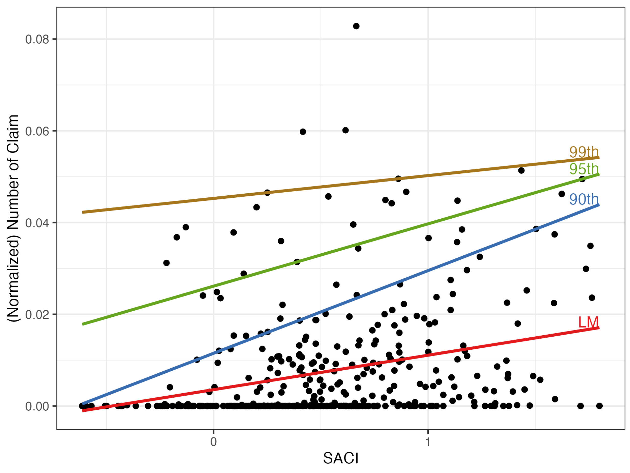
The scatter plot in Figure 8 illustrates the influence of the SACI on the quantiles of N, based on the information in Table 4. The quantile lines correspond to model 4 (Equation (12). With caution, we observe that an increase in the SACI leads to an increase in all three levels of . Additionally, it appears that the higher the probability level, the less steep the quantile line.
In model 5, we introduce the months relevant to hail risk:
while in model 6 we introduce the SACI components together with the months as independent variables:
In Table 5, the results for these two quantile regression models show that both the SACI and its components, except for drought (), significantly impact the normalized number of claims across different quantiles. For the significant variables, confidence intervals lie on either side of the origin. In the cases of , they are on the positive side, indicating an increasing influence on . For , this happens on the negative side, indicating that an increase in the wind component results in a decrease in the corresponding quantile of N (similar to what was observed in the mean of N; see model 3, Equation (11)). These results suggest that the SACI, as a comprehensive climate index, has a substantial impact on the extremes of the number of claims, N. The months constituting the hailstorm season are all significant, as expected. As explained in the previous section, pseudo-R-squared values are calculated following Koenker and Machado (1999). The values obtained for these six models all exceed 0.5, indicating a not negligible fitting score for all these models.
Figure 8.
Scatter plot of the monthly normalized number of claims, N, versus the SACI. Regression and quantile regression (probabilities ) lines corresponding to model 1 (Equation (9), Table 3) and model 4 (Equation (12), Table 4).

Table 5.
Results for quantile regression for the normalized number of claims, N.
| Dependent Variable: | ||||||
|---|---|---|---|---|---|---|
| Number of Claims (Normalized) | ||||||
| Model 5_0.9 | Model 5_0.95 | Model 5_0.99 | Model 6_0.9 | Model 6_0.95 | Model 6_0.99 | |
| SACI | 0.0001 *** | 0.0001 *** | 0.0008 *** | |||
| (0.00003, 0.0001) | (0.0001, 0.0002) | (0.0007, 0.0010) | ||||
| T90std | 0.00003 *** | 0.0002 *** | 0.0017 *** | |||
| (0.00002, 0.00005) | (0.0001, 0.0002) | (0.0015, 0.0019) | ||||
| T10std | 0.0001 *** | 0.0001 ** | 0.0009 *** | |||
| (0.00003, 0.0001) | (0.000003, 0.0002) | (0.0006, 0.0013) | ||||
| Pstd | 0.0001 *** | 0.0003 *** | 0.0019 *** | |||
| (0.00005, 0.0001) | (0.0002, 0.0004) | (0.0015, 0.0022) | ||||
| Dstd | −0.00002 | 0.0001 | 0.0003 | |||
| (−0.0001, 0.00001) | (−0.00002, 0.0002) | (−0.0001, 0.0007) | ||||
| Wstd | −0.00005 *** | −0.0001 *** | −0.0017 *** | |||
| (−0.0001, −0.00003) | (−0.0002, −0.0001) | (−0.0020, −0.0015) | ||||
| Sstd | 0.00002 *** | 0.0001 *** | 0.0008 *** | |||
| (0.00002, 0.00003) | (0.00002, 0.0001) | (0.0007, 0.0010) | ||||
| April | 0.0101 *** | 0.0111 *** | 0.0153 *** | 0.0099 *** | 0.0105 *** | 0.0163 *** |
| (0.0100, 0.0101) | (0.0110, 0.0112) | (0.0150, 0.0156) | (0.0099, 0.0100) | (0.0104, 0.0107) | (0.0157, 0.0169) | |
| May | 0.0264 *** | 0.0600 *** | 0.0817 *** | 0.0265 *** | 0.0596 *** | 0.0798 *** |
| (0.0264, 0.0265) | (0.0599, 0.0601) | (0.0814, 0.0819) | (0.0264, 0.0265) | (0.0594, 0.0598) | (0.0792, 0.0804) | |
| June | 0.0348 *** | 0.0465 *** | 0.0495 *** | 0.0347 *** | 0.0461 *** | 0.0422 *** |
| (0.0347, 0.0348) | (0.0464, 0.0466) | (0.0493, 0.0498) | (0.0346, 0.0347) | (0.0459, 0.0463) | (0.0415, 0.0428) | |
| July | 0.0448 *** | 0.0492 *** | 0.0482 *** | 0.0448 *** | 0.0483 *** | 0.0432 *** |
| (0.0448, 0.0449) | (0.0491, 0.0493) | (0.0480, 0.0485) | (0.0447, 0.0448) | (0.0481, 0.0484) | (0.0426, 0.0439) | |
| August | 0.0373 *** | 0.0455 *** | 0.0589 *** | 0.0372 *** | 0.0449 *** | 0.0572 *** |
| (0.0373, 0.0374) | (0.0454, 0.0456) | (0.0586, 0.0591) | (0.0371, 0.0372) | (0.0448, 0.0451) | (0.0566, 0.0579) | |
| September | 0.0356 *** | 0.0394 *** | 0.0457 *** | 0.0355 *** | 0.0392 *** | 0.0423 *** |
| (0.0356, 0.0357) | (0.0393, 0.0395) | (0.0454, 0.0460) | (0.0355, 0.0356) | (0.0390, 0.0394) | (0.0416, 0.0429) | |
| Constant | 0.00003 *** | 0.0001 *** | 0.0006 *** | 0.0001 *** | 0.0003 *** | 0.0020 *** |
| (0.00001, 0.0001) | (0.00004, 0.0001) | (0.0005, 0.0007) | (0.0001, 0.0001) | (0.0002, 0.0004) | (0.0017, 0.0023) | |
| Observations | 396 | 396 | 396 | 396 | 396 | 396 |
| Pseudo | 0.5607 | 0.5771 | 0.5780 | 0.5609 | 0.5780 | 0.6475 |
Note: * ; ** ; *** .
3.2. Monthly Normalized Number of Loss Costs Equal to One,
Next, we explore the relationship between as the dependent variable and the SACI and its components as independent variables. It is important to note that a claim with a loss cost equal to 1 implies that the loss equals the value of the insured capital, indicating the full scale of damage for that claim.
In model 7, we investigate the linear regression with the SACI alone as an independent variable:
while model 8 also includes the months composing hailstorms season:
Results for both models are presented in Table 6. Model 7 (Equation (15)) indicates that the SACI is statistically significant at the 1% level, with a coefficient of 0.0003. However, the R-squared value is extremely low, , suggesting a very weak explanatory power of the model.
In model 8 (Equation (16)), with the introduction of the months as independent variables (April to September), we observe that only May, July, and August are statistically significant among the month variables. This is a notable difference compared to the case of the number of claims, N, suggesting that not every month in the hailstorm season is relevant to the loss costs being equal to one—only May, July, and August. Overall, the R-squared value of the model increases to 0.146, indicating an improvement in its ability to explain the mean of . In summary, through model 8 (Equation (16)), we have found that the SACI influences, to a certain extent, the mean of . An increase of one unit in the SACI would result in an extremely slight increase in this mean by a factor of 0.0003. Additionally, during the hailstorm season, only May, July, and August are significant for the mean .
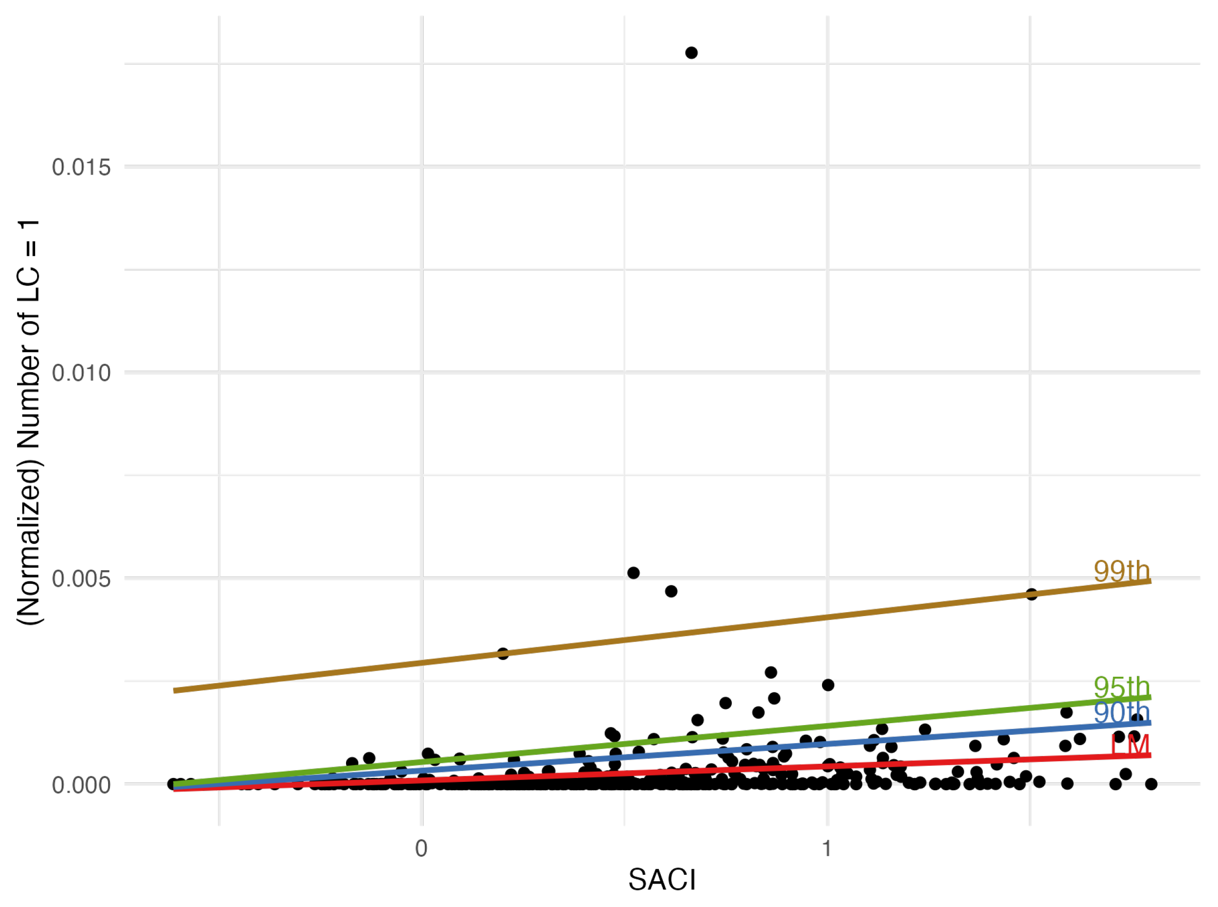
In Figure 9, we observe the increasing line given by model 7 (Equation (15) predicting the mean based on the values of the SACI. Additionally, we find quantile regression lines corresponding to probability levels . In all three cases, we have an increasing line. The three lines correspond to the quantile regression defined by model 9:
In Table 7, the coefficient for the variable SACI is statistically significant at the 1% level for both the 90th and 95th percentiles. This signifies a discernible positive relationship between the SACI and at these percentiles, underscoring its role in influencing . However, at the 99th percentile, there is no significance, and the confidence interval contains zero. This model is relatively weak, as indicated by the very low values of the pseudo-.
Next, in model 10 we introduce the months in the quantile regression using
We have finally decomposed the index into its components, adding the months in the quantile regression model 11 for the same three -values:
Table 7.
Quantile regression results for model 9 (Equation (17).
Table 7.
Quantile regression results for model 9 (Equation (17).
| Dependent Variable: | |||
|---|---|---|---|
| 90th | 95th | 99th | |
| SACI | 0.001 *** | 0.001 *** | 0.001 |
| (0.0004, 0.001) | (0.001, 0.001) | (−0.008, 0.010) | |
| Constant | 0.0003 *** | 0.001 *** | 0.003 |
| (0.0001, 0.001) | (0.0003, 0.001) | (−0.003, 0.009) | |
| Observations | 396 | 396 | 396 |
| Pseudo | 0.0967 | 0.0742 | 0.0411 |
Note: * ; ** ; *** .
Figure 9.
Scatter plot of versus the SACI. The lines represent linear regression and quantile regressions for three different quantiles (0.9, 0.95, and 0.99) corresponding to models 6 and 8.
Figure 9.
Scatter plot of versus the SACI. The lines represent linear regression and quantile regressions for three different quantiles (0.9, 0.95, and 0.99) corresponding to models 6 and 8.

In Table 8, we summarize the results corresponding to models 10 (Equation (18)) and 11 (Equation (19)). In model 10 (Equation (18), the SACI variable has a significant impact on the 95th and 99th quantile levels. All months are significant except April in the 90th and 99th quantiles. In model 11 (19), precipitation, , and drought, , are not significant at any of the three quantile levels, suggesting a weak association between extreme precipitation and drought with extremes. On the other hand, high and low temperatures () are significant variables in all three quantiles, while wind, , and sea level, , are only significant for quantiles and 0.95. Wind coefficients are negative, as observed in previous models. All months from April to September are significant across the three probability levels, and their inclusion has enhanced the models, as indicated by the increase in pseudo- from model 10 to model 11 in Table 7 and Table 8. In this last case, the pseudo- coefficients are all above 0.35, and they increase across higher quantiles, suggesting an improved ability of predictors to capture variability in the number of LC1 at extreme percentiles.
3.3. Monthly Homogenized Losses, L
In the first stage, we will investigate the climate-change effect on L through four linear regression models, examining the impact of the SACI and its components on monthly total hailstorm losses.
Model 12:
Model 13:
Model 14:
Model 15:
The results are presented in Table 9. In models 12 (Equation (20)) and 13 (Equation (21)), the SACI is significant at the 1% confidence level with a positive coefficient, indicating an increase in the mean of L with an increase in the SACI. The for model 12 is not negligible (0.159). Notably, in model 13 we achieve a high value of 0.809, likely attributed to the inclusion of months in this model.
In models 14 (Equation (22)) and 15 (Equation (23)), we explore the significance of SACI components, revealing different levels of significance. In model 14 (without months), hot and cool temperatures, precipitation, and sea level () are significant, while drought and wind ( and ) are not. It is worth noting that the significance of indicates a negative correlation with L. In model 15 (including the months), cool temperatures, wind, and sea level () are significant, while the rest are not. Again, when wind is significant, it is negatively correlated with L. Regarding the scores, it is not negligible for model 14, and in model 15 it achieves a remarkably high value of 0.814. Given the complexity of the models, model 13 provides a more concise explanation of the mean monthly total hailstorm loss than model 15. This is because model 13 consolidates all climate-change effects into one measure, the SACI, simplifying interpretation and understanding.
In the context of model 13, interpreting the SACI coefficient () suggests that an increase of c units in the SACI leads to an increase in the mean of L by . For example, assuming a monthly the SACI increase of 0.1, we would observe an approximate increase in the mean total loss by , equivalent to approximately 9.1%. This interpretation helps estimate the potential cost of future climate change as measured by the SACI. In model 13 (Equation (21)), we calculated the predicted for different SACI values. Choosing the months with the maximum and minimum SACI values among April to September 2022, specifically July 2022 (SACI = 1.764) and May 2022 (SACI = 1.050), the model predicted values were approximately EUR 3,327,700 for July and EUR 2,433,643 for May. These cases can be used to establish upper and lower bounds for the increase in corresponding to a hypothetical future increase in the SACI by 0.1 units. The increase can be estimated by multiplying these values by 0.091:
Change in losses from May to July is not solely attributable to the change in SACI values, as suggested by . Instead, it resulted from a combination of the SACI’s effect and the specific monthly effect encoded by each month’s coefficient, highlighting the model’s complexity. The percentage change in losses due to the month shift, calculated as
which is approximately 36.74%, is approximately 36.74%, demonstrating the significant influence of monthly coefficients on predictions.
Therefore, this interpretation is a key factor for sustainability management because it provides a concrete way to quantify the impact of an increment in the SACI on . In summary, this direct percentage relationship makes the SACI an effective tool for assessing future increases in the mean monthly total loss due to a growing climate-change scenario.
Finally, we note that models 13 and 15 (Equations (21) and (23)), which include the months, demonstrate stronger explanatory power compared to the other two models, as seen from their R-squared values of approximately 0.81.
Next, we move on to the quantile regression models with as the dependent variable. It is relevant to outline here the well-known quantile property (see Koenker 2005, p. 48):
for any monotone transformation, . In our case, .
Model 16 only includes the SACI as an independent variable:
Figure 10 illustrates the relationship between monthly and the SACI. It contains four fitted lines. The upward red line, representing the linear regression, indicates that as the SACI increases, tends to rise also, supporting the conclusion that there is a positive correlation between the SACI and hailstorm losses. In addition, three colored lines correspond to quantile regressions for the 90th, 95th, and 99th percentiles. These lines demonstrate the variation in higher losses associated with SACI values, illustrating the behavior of the tail of the monthly total loss distribution concerning SACI variations. Table 10 presents the results of quantile regression for model 16 (Equation (26), with the dependent variable being and the independent one being the monthly SACI. For the 90th and 95th quantiles, the SACI coefficients are significant at the 1% level. On practical grounds, this implies that a one percentage point of 0.01 increase in the SACI is associated with a 1.141% increase in hail L at the 90th quantile. A similar calculation could be carried out in the 95th quantile. Unfortunately, this is not extensible to the 99th quantile because the coefficient is no longer credible (see its confidence interval and p-value). The pseudo-R-squared values are quite low, implying that the model explains only a small proportion of the variability in hailstorm losses. These values suggest that the SACI independent variable contributes modestly to explaining the variability in hailstorm losses at these quantiles.
In model 17, we include the months of April to September as independent binary variables:
In model 18, we decompose the monthly SACI into its components while still including the months:
Table 11 presents the results of an analysis using quantile regression to investigate the relationship between hailstorm total losses and the SACI or its components. The analysis is conducted separately for the 90th, 95th, and 99th percentiles, taking into account monthly variables from April to September. Concerning model 17 (Equation (27)), the SACI exhibits statistical significance at the three percentiles, even though the confidence interval in the first case contains negative and positive values, a fact that devaluates the quality of this estimate. This indicates (with due caution for the 90th case) a significant positive correlation between the SACI and hailstorm losses across these percentiles. The SACI’s influence becomes more pronounced with increasing percentiles, highlighting its heightened importance in extreme loss events. The observed trend in SACI coefficient values, rising from 0.541 to 0.619, emphasizes its non-uniform impact across quantiles of the monthly total loss distribution. This underscores the SACI’s important role in assessing the severity and potential risk of the most damaging hailstorm events represented in the upper quantiles of the distribution. Note that all the months are significant.
Figure 10.
Scatter plot of monthly versus the SACI. Note: The straight lines are linear regression (see Table 9) and quantile regression () (see Table 10).

Table 10.
Results of quantile regression for model 16 (Equation (26).
Table 10.
Results of quantile regression for model 16 (Equation (26).
| Dependent Variable: | |||
|---|---|---|---|
| 90th | 95th | 99th | |
| SACI | 1.141 *** | 0.963 *** | 0.591 |
| (0.480, 1.802) | (0.467, 1.458) | (−0.274, 1.455) | |
| Constant | 14.031 *** | 14.536 *** | 15.256 *** |
| (13.561, 14.501) | (14.183, 14.888) | (14.641, 15.871) | |
| Observations | 396 | 396 | 396 |
| Pseudo | 0.0319 | 0.0304 | 0.0292 |
Note: * ; ** ; *** .
In model 18 (Equation (28)), (days of extremely hot temperature) is statistically significant at the 95th and 99th percentiles, indicating a positive correlation with losses at higher levels. (days of extremely cold temperature) is only significant at the 95th percentile. (days of heavy rainfall) is significant at the 95th and 99th percentiles. Conversely, (wind speed) has a negative and statistically significant coefficient across all three percentiles, suggesting that higher wind speeds are associated with loss decrease. Remember that a similar behavior was observed for models related to the variables N and .
The variable representing sea level, , is significant at the 90th and 95th quantiles, but not at the 99th one. On the other hand, drought days, , are only significant at the 99th quantile. Note that all the months are significant at all the percentiles.
Table 11.
Results of quantile regression for .
| Dependent Variable: | ||||||
|---|---|---|---|---|---|---|
| Model 17_ = 0.9 | Model 17_ = 0.95 | Model 17_ = 0.99 | Model 18_ = 0.9 | Model 18_ = 0.95 | Model 18_ = 0.99 | |
| SACI | 0.541 * | 0.578 ** | 0.619 *** | |||
| (−0.059, 1.141) | (0.002, 1.153) | (0.257, 0.981) | ||||
| T90std | 0.085 | 0.218 ** | 0.332 *** | |||
| (−0.128, 0.299) | (0.032, 0.404) | (0.183, 0.481) | ||||
| T10std | 0.121 | 0.422 ** | 0.143 | |||
| (−0.268, 0.510) | (0.083, 0.760) | (−0.128, 0.415) | ||||
| Pstd | 0.277 | 0.528 *** | 1.101 *** | |||
| (−0.065, 0.619) | (0.231, 0.826) | (0.863, 1.340) | ||||
| Dstd | 0.169 | 0.066 | 0.876 *** | |||
| (−0.248, 0.587) | (−0.297, 0.429) | (0.585, 1.167) | ||||
| Wstd | −0.338 ** | −0.268 ** | −0.484 *** | |||
| (−0.609, −0.067) | (−0.504, −0.032) | (−0.673, −0.295) | ||||
| Sstd | 0.168 ** | 0.148 ** | 0.020 | |||
| (0.036, 0.300) | (0.033, 0.264) | (−0.073, 0.112) | ||||
| April | 5.331 *** | 4.495 *** | 3.203 *** | 5.165 *** | 4.703 *** | 3.826 *** |
| (4.338, 6.324) | (3.543, 5.447) | (2.604, 3.802) | (4.522, 5.808) | (4.144, 5.263) | (3.378, 4.275) | |
| May | 6.994 *** | 5.857 *** | 4.934 *** | 7.084 *** | 6.077 *** | 5.233 *** |
| (6.015, 7.974) | (4.917, 6.796) | (4.343, 5.525) | (6.453, 7.716) | (5.528, 6.627) | (4.792, 5.673) | |
| June | 6.717 *** | 5.249 *** | 3.911 *** | 6.594 *** | 5.672 *** | 4.694 *** |
| (5.702, 7.732) | (4.275, 6.222) | (3.299, 4.523) | (5.889, 7.299) | (5.059, 6.285) | (4.202, 5.185) | |
| July | 7.003 *** | 5.715 *** | 3.955 *** | 6.657 *** | 5.707 *** | 4.560 *** |
| (5.998, 8.008) | (4.750, 6.679) | (3.348, 4.561) | (5.970, 7.344) | (5.109, 6.305) | (4.081, 5.039) | |
| August | 6.767 *** | 5.388 *** | 3.625 *** | 6.387 *** | 5.317 *** | 3.719 *** |
| (5.759, 7.776) | (4.420, 6.355) | (3.017, 4.234) | (5.720, 7.054) | (4.737, 5.897) | (3.253, 4.184) | |
| September | 6.687 *** | 5.420 *** | 3.639 *** | 6.622 *** | 5.624 *** | 4.528 *** |
| (5.700, 7.675) | (4.473, 6.367) | (3.043, 4.235) | (5.940, 7.303) | (5.032, 6.217) | (4.052, 5.003) | |
| Constant | 7.992 *** | 9.540 *** | 11.305 *** | 8.142 *** | 9.439 *** | 11.018 *** |
| (7.570, 8.414) | (9.135, 9.945) | (11.050, 11.560) | (7.854, 8.430) | (9.189, 9.690) | (10.817, 11.219) | |
| Observations | 396 | 396 | 396 | 396 | 396 | 396 |
| Pseudo | 0.3711 | 0.3192 | 0.2531 | 0.38 | 0.3354 | 0.2857 |
Note: * ; ** ; *** .
Let us consider model 17 in the case of (Equation (27). Let us also consider again the maximum and minimum SACI monthly values for 2022, which are 1.764 (July) and 1.050 (May). We aim to build two bounds (relatives to the year 2022) for the L-99th quantile variation corresponding to an SACI variation of 0.1, as was done for its mean in (24). Model 17 predictions for the L-99th quantiles corresponding to those SACI values are, respectively:
The two 2022-bounds for the L-99th quantile variation corresponding to a 0.1 increase in the SACI are:
Observe that, when increasing the SACI by 0.1, the adjustment in the 99th quantile of L can be computed by simply multiplying the loss by , which is approximately 1.0639. Again, as in (24), this interpretation is a key factor for sustainability management because it potentially provides a concrete way to quantify the impact of an increment in the SACI into any -quantile of the monthly total loss, L. This direct percentage relationship makes the SACI an effective tool for assessing future increases in any quantile of L caused by an increasing climate-change scenario.
4. Discussion
In this paper, we explore the relationship between the Spanish Actuarial Climate Index (SACI) and its components and hailstorm insurance claims in Spanish agricultural insurance, in the line of business of wine grapes. Insurance claims are represented by the monthly number of claims, monthly number of loss costs equal to one, and monthly total losses observed from 1990 to 2022, and the methodologies we use are linear and quantile regression models.
Until now, the influence of climate change on hailstorm risk has been scarcely studied, lacking the systematic approach achieved through our quantification of climate change using the SACI. As mentioned in the introduction, Raupach et al. (2021) suggests a potential increase in hailstorms in Europe, albeit without a specific connection to insurance. In a study by Botzen et al. (2010), Tobit regressions were employed to investigate the relationship between climate change and hailstorm insurance damages for greenhouse horticulture and outdoor farming. The primary finding was that a combination of maximum temperatures and precipitation best predicts hailstorm damage, projecting a considerable increase in future hailstorm damage.
Our study enhances precision and conciseness by representing climate change through our climate index, providing a more compact and summarized representation while retaining the ability to analyze the influence of any variable comprising the index (see models 2, 3, 6, 11, 14, 15, 18). Through these models, we conclude that there is no simple rule or organized pattern describing these individual influences. Their significance can vary or even disappear from expectations to high quantiles or even between quantiles close to one another. We observe that, in general, the regression coefficients are positive, except for the wind component, which exhibits a negative slope whenever it is significant.
We believe we are the first to apply both linear and quantile regression to investigate the influence of the climate index and its components on hailstorm risk insurance. These methodologies allow us to address the crucial open question of estimating the future cost of climate change.
Our results indicate a significant positive correlation between the SACI and the three dependent variables. Its explanatory power is relatively high for some models relative to the monthly total losses, L (models 13 to 18, Table 9, Table 10 and Table 11), the monthly number of loss costs equal to one (models 10 and 11, Table 8), and the monthly normalized number of claims (models (13) and (14), Table 5).
Importantly, we show that these two methodologies can be key factors in the assessment and management of hailstorm risk because they provide estimations of the growth of expectations and quantiles of the claims and loss variables corresponding to future shifts in climate change as measured by the Spanish Actuarial Climate Index (SACI) (see Equations (24), (29), and (30)).
5. Conclusions
We have assessed the impact of climate change on hailstorm risk in Spanish wine grape crop insurance through the application of a range of extreme weather variables forming a climate index (SACI), employing linear and quantile regression methodologies. Importantly, we have monetarily quantified this impact, corresponding to a future increase of one basis point (0.1) in the SACI. This calculation involves estimating the increases in both expected and quantile total monthly losses.
Many of the results of our calculations may be directly translated to premium and solvency capital calculations, providing an efficient tool for guaranteeing the sustainability of the insurance business against climate change.
Future research endeavors will seek to expand this strategy to other insurance markets and explore risk measures beyond the expectation and Value at Risk (VaR). In the context of wine grape crop insurance, there is potential to broaden this study by tailoring its conclusions to each province, geographically specifying the regions most threatened by this risk, and quantifying the local costs associated with a future rise in the climate index.
Author Contributions
N.Z.and J.L.V.-Z. equally contributed to this research; funding acquisition, J.L.V.-Z. All authors have read and agreed to the published version of the manuscript.
Funding
This research was funded by the Spanish Government’s Ministry of Science and Innovation, grant numbers PID2020-115700RB-I00 and PID2021-125133NB-I00.
Data Availability Statement
The database is the property of AGROSEGURO S.A.
Conflicts of Interest
The authors declare no conflicts of interest. The funders had no role in the design of the study; in the collection, analyses, or interpretation of data; in the writing of the manuscript; or in the decision to publish the results.
Abbreviations
The following abbreviations are used in this manuscript:
| ACI | Actuaries Climate Index™ |
| IACI | Iberian Actuarial Climate Index |
| SACI | Spanish Actuarial Climate Index |
References
- ACI. 2018. Actuaries Climate Index: Development and Design. Available online: https://actuariesclimateindex.org/wp-content/uploads/2019/05/ACI.DevDes.2.20.pdf (accessed on 15 January 2024).
- Agroseguro. 2023. Available online: https://agroseguro.es/en/ (accessed on 22 December 2023).
- Al-Maruf, Abdullah, Sumyia Akter Mira, Tasnim Nazira Rida, Md Saifur Rahman, Pradip Kumar Sarker, and J. Craig Jenkins. 2021. Piloting a weather-index-based crop insurance system in Bangladesh: Understanding the challenges of financial instruments for tackling climate risks. Sustainability 13: 8616. [Google Scholar] [CrossRef]
- AP. 2023. California Insurance Market Rattled by Withdrawal of Major Companies. Available online: https://apnews.com/article/california-wildfire-insurance-e31bef0ed7eeddcde096a5b8f2c1768f (accessed on 18 December 2023).
- Baione, Fabio, and Davide Biancalana. 2021. An application of parametric quantile regression to extend the two-stage quantile regression for rate making. Scandinavian Actuarial Journal 2021: 156–70. [Google Scholar] [CrossRef]
- Barthel, Fabian, and Eric Neumayer. 2012. A trend analysis of normalized insured damage from natural disasters. Climatic Change 113: 215–37. [Google Scholar] [CrossRef]
- Benoit, Kenneth. 2011. Linear regression models with logarithmic transformations. London School of Economics, London 22: 23–36. [Google Scholar]
- Botzen, W. J. W., L. M. Bouwer, and J. C. J. M. Van den Bergh. 2010. Climate change and hailstorm damage: Empirical evidence and implications for agriculture and insurance. Resource and Energy Economics 32: 341–62. [Google Scholar] [CrossRef]
- Charpentier, Arthur. 2008. Insurability of climate risks. The Geneva Papers on Risk and Insurance-Issues and Practice 33: 91–109. [Google Scholar] [CrossRef]
- Courbage, Courbage, and Maryam Golnaraghi. 2022. Extreme events, climate risks and insurance. The Geneva Papers on Risk and Insurance-Issues and Practice 47: 1–4. [Google Scholar] [CrossRef]
- De Jong, Piet, and Gillian Z. Heller. 2008. Generalized Linear Models for Insurance Data. Cambridge, UK: Cambridge University Press. [Google Scholar]
- Denuit, Michel, Xavier Maréchal, Sandra Pitrebois, and Jean-François Walhin. 2007. Actuarial Modeling of Claim Counts: Risk Classification, Credibility and Bonus-Malus Systems. New York: John Wiley & Sons. [Google Scholar]
- Dundon, Leah A., Katherine S. Nelson, Janey Camp, Mark Abkowitz, and Alan Jones. 2016. Using climate and weather data to support regional vulnerability screening assessments of transportation infrastructure. Risks 4: 28. [Google Scholar] [CrossRef]
- Heranval, Antoine, Olivier Lopez, and Maud Thomas. 2022. Application of machine learning methods to predict drought cost in France. European Actuarial Journal 13: 1–23. [Google Scholar] [CrossRef]
- Heras, Antonio, Ignacio Moreno, and José L. Vilar-Zanón. 2018. An application of two-stage quantile regression to insurance rate making. Scandinavian Actuarial Journal 2018: 753–69. [Google Scholar] [CrossRef]
- Jørgensen, Sisse Liv, Mette Termansen, and Unai Pascual. 2020. Natural insurance as condition for market insurance: Climate change adaptation in agriculture. Ecological Economics 169: 106489. [Google Scholar] [CrossRef]
- Koenker, Roger. 2005. Quantile Regression. Cambridge, UK: Cambridge University Press. [Google Scholar]
- Koenker, Roger. 2015. Quantreg: Quantile Regression. R Package Version 5.97. Available online: http://CRAN.R-project.org/package=quantreg (accessed on 19 January 2024).
- Koenker, Roger, and Gilbert Bassett Jr. 1978. Regression quantiles. Econometrica: Journal of the Econometric Society 23: 33–50. [Google Scholar] [CrossRef]
- Koenker, Roger, and Jose A. F. Machado. 1999. Goodness of fit and related inference processes for quantile regression. Journal of the American Statistical Association 94: 1296–310. [Google Scholar] [CrossRef]
- Lemaire, Jean. 2012. Bonus-Malus Systems in Automobile Insurance. New York: Springer Science and Business Media, vol. 19. [Google Scholar]
- Li, Han, and Qihe Tang. 2022. Joint extremes in temperature and mortality: A bivariate POT approach. North American Actuarial Journal 26: 43–63. [Google Scholar] [CrossRef]
- Lyubchich, Vyacheslav, K. Newlands Newlands, Azar Ghahari, Tahir Mahdi, and Yulia R. Gel. 2019. Insurance risk assessment in the face of climate change: Integrating data science and statistics. Wiley Interdisciplinary Reviews: Computational Statistics 11: e1462. [Google Scholar] [CrossRef]
- Miljkovic, Tatjana, Dragan Miljkovic, and Karsten Maurer. 2018. Examining the impact on mortality arising from climate change: Important findings for the insurance industry. European Actuarial Journal 8: 363–81. [Google Scholar] [CrossRef]
- Niall, Stephanie, and Kevin Walsh. 2005. The impact of climate change on hailstorms in southeastern Australia. International Journal of Climatology: A Journal of the Royal Meteorological Society 25: 1933–52. [Google Scholar] [CrossRef]
- Pielke, Roger A., and Christopher W. Landsea. 1998. Normalized Hurricane Damages in the United States: 1925–95. Weather and Forecasting 13: 621–31. [Google Scholar] [CrossRef]
- Portmann, Raphael, Timo Schmid, Leonie Villiger, David N. Bresch, and Pierluigi Calanca. 2023. Modelling crop hail damage footprints with single-polarization radar: The roles of spatial resolution, hail intensity, and cropland density. EGUsphere, 1–29. [Google Scholar]
- Pryor, Louise. 2017. The Impacts of Climate Change on Health. London: Institute & the Faculty of Actuaries. [Google Scholar]
- Rao, Shuling, and Xinhang Li. 2023. China’s Experiences in Climate Risk Insurance and Suggestions for Its Future Development. In Annual Report on Actions to Address Climate Change (2019) Climate Risk Prevention. Berlin: Springer, pp. 157–71. [Google Scholar]
- Raupach, Timothy H., Olivia Martius, John T. Allen, Michael Kunz, Sonia Lasher-Trapp, Susanna Mohr, Kristen L. Rasmussen, Robert J. Trapp, and Qinghong Zhang. 2021. The effects of climate change on hailstorms. Nature Reviews Earth & Environment 2: 213–26. [Google Scholar]
- Reyes, Julian, Emile Elias, Erin Haacker, Amy Kremen, Lauren Parker, and Caitlin Rottler. 2020. Assessing agricultural risk management using historic crop insurance loss data over the Ogallala aquifer. Agricultural Water Management 232: 106000. [Google Scholar] [CrossRef]
- Savitz, Ryan, and Marius Dan Gavriletea. 2019. Climate change and insurance. Transformations in Business & Economics 18: 21. [Google Scholar]
- Simbürger, Markus, Sabrina Dreisiebner-Lanz, Michael Kernitzkyi, and Franz Prettenthaler. 2022. Climate risk management with insurance or tax-exempted provisions? An empirical case study of hail and frost risk for wine and apple production in Styria. International Journal of Disaster Risk Reduction 80: 103216. [Google Scholar] [CrossRef]
- Statista. 2023. Vineyard Surface Area in European Countries in 2022. Available online: https://www.statista.com/statistics/1247482/vineyard-surface-area-europe/ (accessed on 20 December 2023).
- Thistlethwaite, Jason, and Michael O. Wood. 2018. Insurance and climate change risk management: Rescaling to look beyond the horizon. British Journal of Management 29: 279–98. [Google Scholar] [CrossRef]
- UN. 2023. What Is Climate Change? Available online: https://www.un.org/en/climatechange/what-is-climate-change (accessed on 18 December 2023).
- Vilar-Zanón, José L., Antonio Heras, and Estela de Frutos. 2020. An average model approach to experience based premium rates discounts: An application to Spanish agricultural insurance. European Actuarial Journal 10: 361–75. [Google Scholar]
- Wagner, Katherine R. H. 2022. Designing insurance for climate change. Nature Climate Change 12: 1070–72. [Google Scholar] [CrossRef]
- Warren-Myers, Georgia, Gideon Aschwanden, Franz Fuerst, and Andy Krause. 2018. Estimating the potential risks of sea level rise for public and private property ownership occupation and management. Risks 6: 37. [Google Scholar] [CrossRef]
- Weisberg, Sanford. 2005. Applied Linear Regression. New York: John Wiley & Sons, vol. 528. [Google Scholar]
- Zhou, Nan, José-Luis Vilar-Zanón, José Garrido, and Antonio-José Heras Martínez. 2023. On the definition of an actuarial climate index for the Iberian peninsula. Anales del Instituto de Actuarios Españoles, 37–59. [Google Scholar] [CrossRef]
Figure 2.
Yearly normalized number of hailstorm claims and its linear trend.

Figure 3.
Monthly number of claims (normalized) from January 1990 to December 2022.

Figure 4.
Yearly normalized .

Figure 5.
Monthly total losses for the period January 1990–December 2022. The light blue points are the homogeneous losses and the dark blue points are their logarithms.
Figure 5.
Monthly total losses for the period January 1990–December 2022. The light blue points are the homogeneous losses and the dark blue points are their logarithms.

Figure 6.
Yearly total loss quantiles .

Figure 7.
Annual SACI variation from April to September (1961–2022) as an indicator of climate change during the hailstorm season.
Figure 7.
Annual SACI variation from April to September (1961–2022) as an indicator of climate change during the hailstorm season.

Table 4.
Quantile regression results for model 4 (Equation (12)).
Table 4.
Quantile regression results for model 4 (Equation (12)).
| Dependent Variable: | |||
|---|---|---|---|
| Number of Claim (Normalized) | |||
| = 0.9 | = 0.95 | = 0.99 | |
| SACI | 0.018 *** | 0.014 | 0.005 * |
| (0.013, 0.023) | (−0.004, 0.031) | (−0.001, 0.011) | |
| Constant | 0.012 *** | 0.026 *** | 0.045 *** |
| (0.008, 0.015) | (0.014, 0.038) | (0.041, 0.049) | |
| Observations | 396 | 396 | 396 |
| Pseudo | 0.0928 | 0.0420 | 0.0173 |
Note: * ; ** ; *** .
Table 6.
Linear regression for number of loss cost = 1.
| Dependent Variable: | ||
|---|---|---|
| Number of Claims (Loss Cost = 1) | ||
| Model 7 | Model 8 | |
| SACI | 0.0003 *** | 0.0002 * |
| (0.0001) | (0.0001) | |
| April | −0.00001 | |
| (0.0002) | ||
| May | 0.001 *** | |
| (0.0002) | ||
| June | 0.0003 | |
| (0.0002) | ||
| July | 0.001 *** | |
| (0.0002) | ||
| August | 0.0004 ** | |
| (0.0002) | ||
| September | 0.0002 | |
| (0.0002) | ||
| Constant | 0.0001 | −0.0001 |
| (0.0001) | (0.0001) | |
| Observations | 396 | 396 |
| R2 | 0.024 | 0.146 |
| Adjusted R2 | 0.021 | 0.131 |
| Residual Std. Error | 0.001 (df = 394) | 0.001 (df = 388) |
| F Statistic | 9.608 *** (df = 1; 394) | 9.475 *** (df = 7; 388) |
Note: * ; ** ; *** .
Table 8.
Quantile regression results for .
| Dependent Variable: | ||||||
|---|---|---|---|---|---|---|
| Number of (Normalized) | ||||||
| Mod 10 | Mod 10 | Mod 10 | Mod 11 | Mod 11 | Mod 11 | |
| SACI | 0.000 | 0.00000 *** | 0.0003 *** | |||
| (−0.0003, 0.0003) | (0.00000, 0.00001) | (0.0002, 0.0003) | ||||
| T90std | 0.004 *** | 0.010 *** | 0.016 *** | |||
| (0.003, 0.004) | (0.009, 0.011) | (0.016, 0.017) | ||||
| T10std | 0.001 ** | 0.004 *** | 0.003 *** | |||
| (0.0001, 0.002) | (0.002, 0.006) | (0.001, 0.004) | ||||
| Pstd | 0.0001 | 0.0001 | 0.0001 | |||
| (−0.001, 0.001) | (−0.002, 0.002) | (−0.001, 0.001) | ||||
| Dstd | −0.0004 | 0.0002 | −0.001 | |||
| (−0.002, 0.001) | (−0.002, 0.002) | (−0.002, 0.001) | ||||
| Wstd | −0.002 *** | −0.003 *** | −0.001 | |||
| (−0.003, −0.001) | (−0.004, −0.001) | (−0.002, 0.0002) | ||||
| Sstd | 0.001 *** | 0.002 *** | −0.0001 | |||
| (0.001, 0.001) | (0.001, 0.003) | (−0.001, 0.0003) | ||||
| April | 0.0002 | 0.0002 *** | 0.0001 | 0.013 *** | 0.008 *** | 0.005 *** |
| (−0.0002, 0.001) | (0.0002, 0.0002) | (−0.0001, 0.0002) | (0.011, 0.015) | (0.005, 0.011) | (0.003, 0.007) | |
| May | 0.003 *** | 0.005 *** | 0.017 *** | 0.314 *** | 0.493 *** | 1.760 *** |
| (0.003, 0.004) | (0.005, 0.005) | (0.017, 0.018) | (0.313, 0.316) | (0.490, 0.497) | (1.758, 1.762) | |
| June | 0.001 *** | 0.001 *** | 0.001 *** | 0.096 *** | 0.102 *** | 0.106 *** |
| (0.001, 0.002) | (0.001, 0.001) | (0.001, 0.001) | (0.094, 0.098) | (0.098, 0.105) | (0.104, 0.109) | |
| July | 0.002 *** | 0.003 *** | 0.004 *** | 0.134 *** | 0.248 *** | 0.403 *** |
| (0.001, 0.002) | (0.003, 0.003) | (0.004, 0.004) | (0.131, 0.136) | (0.245, 0.251) | (0.401, 0.405) | |
| August | 0.001 *** | 0.002 *** | 0.002 *** | 0.095 *** | 0.123 *** | 0.168 *** |
| (0.001, 0.002) | (0.002, 0.002) | (0.002, 0.002) | (0.092, 0.097) | (0.119, 0.126) | (0.166, 0.170) | |
| September | 0.001 *** | 0.001 *** | 0.002 *** | 0.061 *** | 0.122 *** | 0.183 *** |
| (0.0002, 0.001) | (0.001, 0.001) | (0.002, 0.002) | (0.059, 0.063) | (0.119, 0.126) | (0.181, 0.186) | |
| Constant | 0.000 | 0.00000 ** | 0.0002 *** | 0.002 *** | 0.005 *** | 0.012 *** |
| (−0.0002, 0.0002) | (0.00000, 0.00000) | (0.0001, 0.0002) | (0.001, 0.003) | (0.004, 0.007) | (0.011, 0.013) | |
| Observations | 396 | 396 | 396 | 396 | 396 | 396 |
| Pseudo | 0.3559 | 0.4101 | 0.7156 | 0.3585 | 0.4150 | 0.7275 |
Note: * ; ** ; *** .
Table 9.
Results of linear regression models for .
| Dependent Variable: | ||||
|---|---|---|---|---|
| Model 12 | Model 13 | Model 14 | Model 15 | |
| SACI | 5.350 *** | 0.878 *** | ||
| (0.620) | (0.327) | |||
| T90std | 0.737 ** | 0.226 | ||
| (0.331) | (0.180) | |||
| T10std | 1.204 * | 0.621 * | ||
| (0.640) | (0.328) | |||
| Pstd | −2.350 *** | 0.023 | ||
| (0.532) | (0.289) | |||
| Dstd | −0.312 | 0.414 | ||
| (0.692) | (0.352) | |||
| Wstd | 0.723 | −0.388 * | ||
| (0.442) | (0.229) | |||
| Sstd | 1.759 *** | 0.344 *** | ||
| (0.195) | (0.112) | |||
| April | 9.371 *** | 9.214 *** | ||
| (0.541) | (0.542) | |||
| May | 11.861 *** | 11.863 *** | ||
| (0.533) | (0.533) | |||
| June | 11.066 *** | 10.852 *** | ||
| (0.553) | (0.595) | |||
| July | 11.547 *** | 11.360 *** | ||
| (0.547) | (0.580) | |||
| August | 11.482 *** | 11.385 *** | ||
| (0.549) | (0.562) | |||
| September | 11.028 *** | 10.853 *** | ||
| (0.538) | (0.575) | |||
| Constant | 5.083 *** | 1.922 *** | 4.444 *** | 1.925 *** |
| (0.441) | (0.230) | (0.454) | (0.243) | |
| Observations | 396 | 396 | 396 | 396 |
| R2 | 0.159 | 0.809 | 0.266 | 0.814 |
| Adjusted R2 | 0.157 | 0.805 | 0.255 | 0.808 |
| Residual Std. Error | 5.859 (df = 394) | 2.815 (df = 388) | 5.509 (df = 389) | 2.794 (df = 383) |
| F Statistic | 74.511 *** (df = 1; 394) | 234.536 *** (df = 7; 388) | 23.497 *** (df = 6; 389) | 139.809 *** (df = 12; 383) |
Note: * ; ** ; *** .
Disclaimer/Publisher’s Note: The statements, opinions and data contained in all publications are solely those of the individual author(s) and contributor(s) and not of MDPI and/or the editor(s). MDPI and/or the editor(s) disclaim responsibility for any injury to people or property resulting from any ideas, methods, instructions or products referred to in the content. |
© 2024 by the authors. Licensee MDPI, Basel, Switzerland. This article is an open access article distributed under the terms and conditions of the Creative Commons Attribution (CC BY) license (https://creativecommons.org/licenses/by/4.0/).
Share and Cite
MDPI and ACS Style
Zhou, N.; Vilar-Zanón, J.L. Impact Assessment of Climate Change on Hailstorm Risk in Spanish Wine Grape Crop Insurance: Insights from Linear and Quantile Regressions. Risks 2024, 12, 20. https://doi.org/10.3390/risks12020020
AMA Style
Zhou N, Vilar-Zanón JL. Impact Assessment of Climate Change on Hailstorm Risk in Spanish Wine Grape Crop Insurance: Insights from Linear and Quantile Regressions. Risks. 2024; 12(2):20. https://doi.org/10.3390/risks12020020
Chicago/Turabian StyleZhou, Nan, and José L. Vilar-Zanón. 2024. "Impact Assessment of Climate Change on Hailstorm Risk in Spanish Wine Grape Crop Insurance: Insights from Linear and Quantile Regressions" Risks 12, no. 2: 20. https://doi.org/10.3390/risks12020020
Note that from the first issue of 2016, this journal uses article numbers instead of page numbers. See further details here.