
One-Machine Scheduling with Time-Dependent Capacity via Efficient Memetic Algorithms

Department of Computer Science, University of Oviedo, 33204 Gijón, Spain
*
Author to whom correspondence should be addressed.
Mathematics 2021, 9(23), 3030; https://doi.org/10.3390/math9233030
Submission received: 12 October 2021
/
Revised: 19 November 2021
/
Accepted: 22 November 2021
/
Published: 26 November 2021
(This article belongs to the Special Issue Advances in Artificial Intelligence and Metaheuristics Methods for Planning and Scheduling)
Abstract
:This paper addresses the problem of scheduling a set of jobs on a machine with time-varying capacity, with the goal of minimizing the total tardiness objective function. This problem arose in the context scheduling the charging times of a fleet of electric vehicles and it is NP-hard. Recent work proposed an efficient memetic algorithm for solving the problem, combining a genetic algorithm and a local search method. The local search procedure is based on swapping consecutive jobs on a C-path, defined as a sequence of consecutive jobs in a schedule. Building on it, this paper develops new memetic algorithms that stem from new local search procedures also proposed in this paper. The local search methods integrate several mechanisms to make them more effective, including a new condition for swapping pairs of jobs, a hill climbing approach, a procedure that operates on several C-paths and a method that interchanges jobs between different C-paths. As a result, the new local search methods enable the memetic algorithms to reach higher-quality solutions. Experimental results show significant improvements over existing approaches.
1. Introduction
Over the last few decades, scheduling problems have become ubiquitous in a growing number of domains, including manufacturing, transportation or cloud computing, among others [1,2]. These problems often exhibit a high computational complexity [3,4,5,6], what makes them an interesting subject of study to several scientific disciplines, as artificial intelligence, operations research or applied mathematics. As a consequence, numerous solving methods, both exact and approximate, have been proposed in the literature, capable of solving increasingly challenging problems.
Exact methods include branch and bound algorithms [7,8], constraint programming [9] or mathematical programming approaches [10], among others.
On the other hand, efficient metaheuristic algorithms have been proposed with the aim of computing high-quality solutions in short time. In this respect, genetic algorithms (GAs) stand out as very effective population-based metaheuristics. These algorithms evolve a population of solutions by means of selection, recombination and replacement genetic operators. GAs have been used to solve numerous scheduling problems, including one-machine [11], parallel machines [12], job shop [13] or resource constrained project scheduling problems [14]. In addition, local search approaches have been widely used in this domain (e.g., to solve one-machine [15], job shop [16] or Earth observation satellite scheduling problems [17], to name a few). In contrast to population-based metaheuristics, these methods work on a single solution, iteratively introducing changes on it to improve its quality. Local search methods have been successfully combined with other metaheuristics as genetic algorithms, resulting in so-called memetic algorithms (MAs). These algorithms have been shown to achieve a proper balance between the exploration and exploitation of the search space, what makes them more effective at solving different scheduling problems, as one-machine [18] or flow shop scheduling problems [19].
Other successful metaheuristics include, among others, differential evolution (DE) [20], ant colony optimization (ACO) [21] or particle swarm optimization (PSO) [22]. In addition, recent work explored hybrid methods combining metaheuristics and machine learning in different domains [23,24].
One-machine scheduling problems have played an important role in scheduling. In general, these problems require scheduling a set of jobs on a unique resource, satisfying diverse constraints, with the goal of optimizing a given objective function. In addition to their many practical applications (e.g., supply chain [25], packet-switched networks [26], or manufacturing [27]), they stand out for acting as building blocks of other more complex problems, usually providing useful approximations or lower bounds [7,28].
This paper studies a problem of this kind that arose in the context of scheduling the charging times of a fleet of electric vehicles [29]. In its formal definition, a set of jobs has to be scheduled on a single machine whose capacity varies over time, with the aim of minimizing the total tardiness objective function. This problem is denoted in the conventional notation [30] and it is NP-hard [31,32].
The problem has been considered both in online (with real-time requirements) and offline settings. In [29], it was solved by means of the Apparent Tardiness Cost (ATC) priority rule [33], which is of common use in scheduling problems with tardiness objectives. Later, a genetic algorithm [31] was shown to compute much better schedules than classical priority rules, including ATC, at the expense of longer running times. More recently, this genetic algorithm was combined with an efficient local search procedure, resulting in a memetic algorithm [32]. The local search method is based on swapping pairs of consecutive jobs in a so-called C-path, defined as a sequence of consecutive jobs in a feasible schedule. The memetic algorithm was shown to outperform the genetic algorithm by a wide margin and, to our best knowledge, it is the current best-performing offline approach for solving the problem. The problem has also been solved in the recent past by means of priority rules evolved by genetic programming [34], as well as ensembles (or sets) of rules [35]. These approaches often produce better schedules than classical rules, as ATC, and are well-suited for solving the problem online, given their very short running times. However, the quality of the schedules they compute was shown to be still significantly lower than that of the schedules calculated by offline methods, as the aforementioned memetic algorithm.
Building on [32], this paper makes several contributions towards solving the problem:
- •
- First, new efficient local search procedures for the problem are proposed and their relevant properties, as correctness and worst-case complexity, are studied. As the previous local search approach, the new methods rely on the notion of C-paths in a feasible schedule. However, they incorporate mechanisms to make them more effective. These include a new condition for swapping pairs of consecutive jobs, the integration of a hill climbing approach, a procedure that operates on several C-paths at the same time and a new way of improving the quality of schedules by interchanging jobs between different C-paths.
- •
- Then, the local search procedures are exploited in combination with a genetic algorithm, giving rise to new memetic algorithms. These algorithms have been designed with the aim of achieving a proper balance between the exploration of the search space and the intensification in its most promising areas.
- •
- An extensive experimental study demonstrates that the memetic algorithms proposed in this work achieve conclusive improvements in practice. The results reveal that the new local search procedures enable the memetic algorithms to reach far better solutions than other methods, including the memetic algorithm proposed in [32] and a constraint programming approach.
The remainder of the paper is structured as follows: Section 2 formally defines the problem. Section 3 summarizes the main components of the memetic algorithm proposed in [32], providing the necessary background. The new local search procedures and the new memetic algorithms are described in Section 4 and Section 5, respectively. Section 6 reports the results from the experimental study. Finally, the paper concludes in Section 7.
2. Definition of the Problem
In the problem n jobs have to be scheduled on a single machine. Each job is available at time and has a given duration and a due date . Processing a job results in the consumption of one unit of the machine’s capacity while it is being processed. The capacity of the machine varies over time: for a time instant , denotes its capacity in the interval . It is assumed that for all .
A feasible schedule S is an assignment of a starting time to each job satisfying the following constraints:
- The capacity of the machine cannot be exceeded at any time, i.e., for all , where denotes the total consumption of the machine in the interval due to the jobs scheduled. This corresponds to the number of jobs that are processed in parallel in that interval.
- The processing of a job cannot be preempted, i.e., for all , where denotes the completion time of job i.
In a feasible schedule S, each job incurs in a tardiness , which measures its delay when the job is completed after its due date. The total tardiness of S, denoted , is defined as the sum of the tardiness values of all the jobs, that is:
The goal is to find a feasible schedule with the minimum total tardiness possible.
Example 1.
Consider a problem instance with a set of jobs , whose durations and due dates are given in the following table:
| i | 1 | 2 | 3 | 4 | 5 | 6 | 7 | 8 | 9 | 10 | 11 | 12 |
| 4 | 4 | 2 | 3 | 4 | 3 | 2 | 3 | 2 | 3 | 3 | 5 | |
| 4 | 9 | 13 | 4 | 7 | 8 | 10 | 3 | 13 | 5 | 9 | 7 |
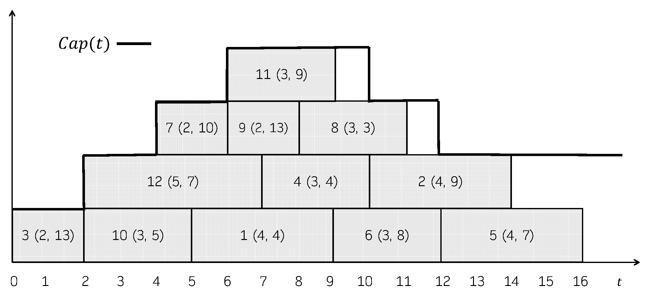
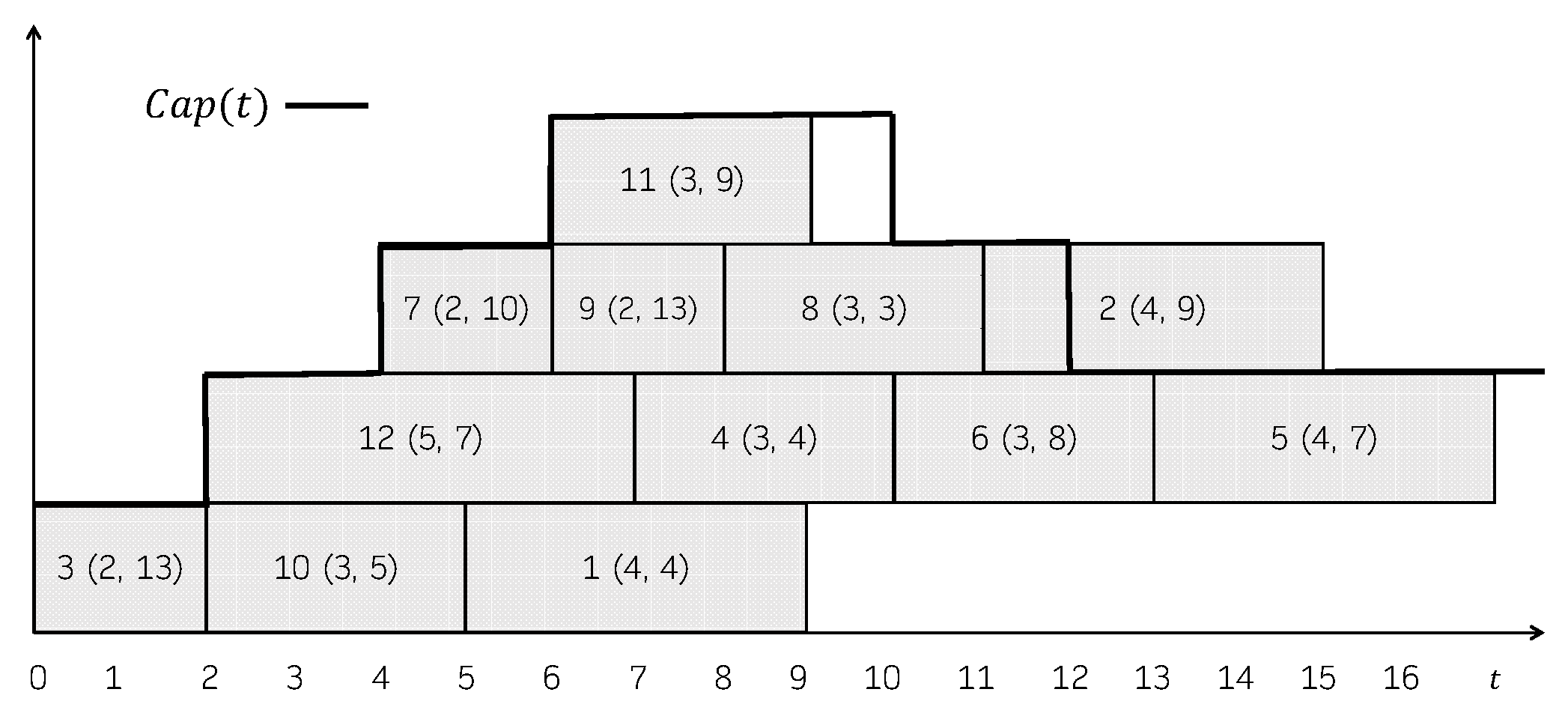
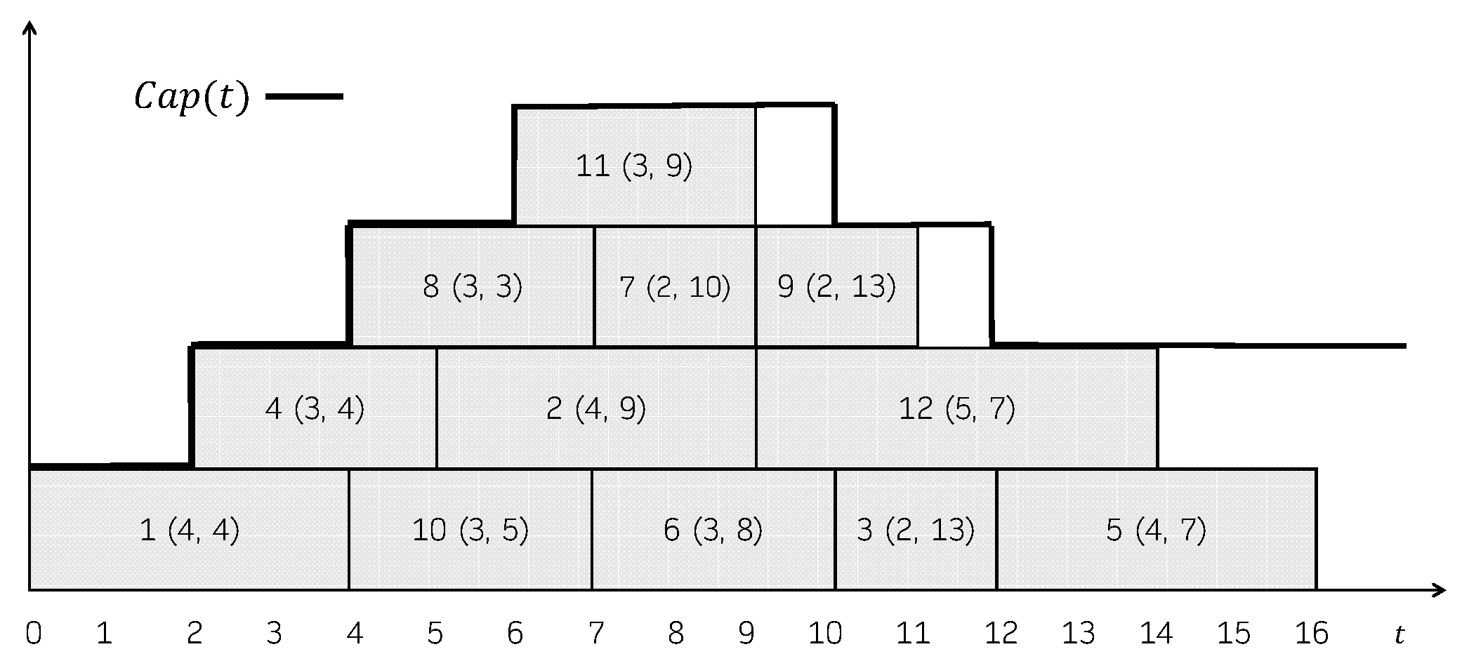
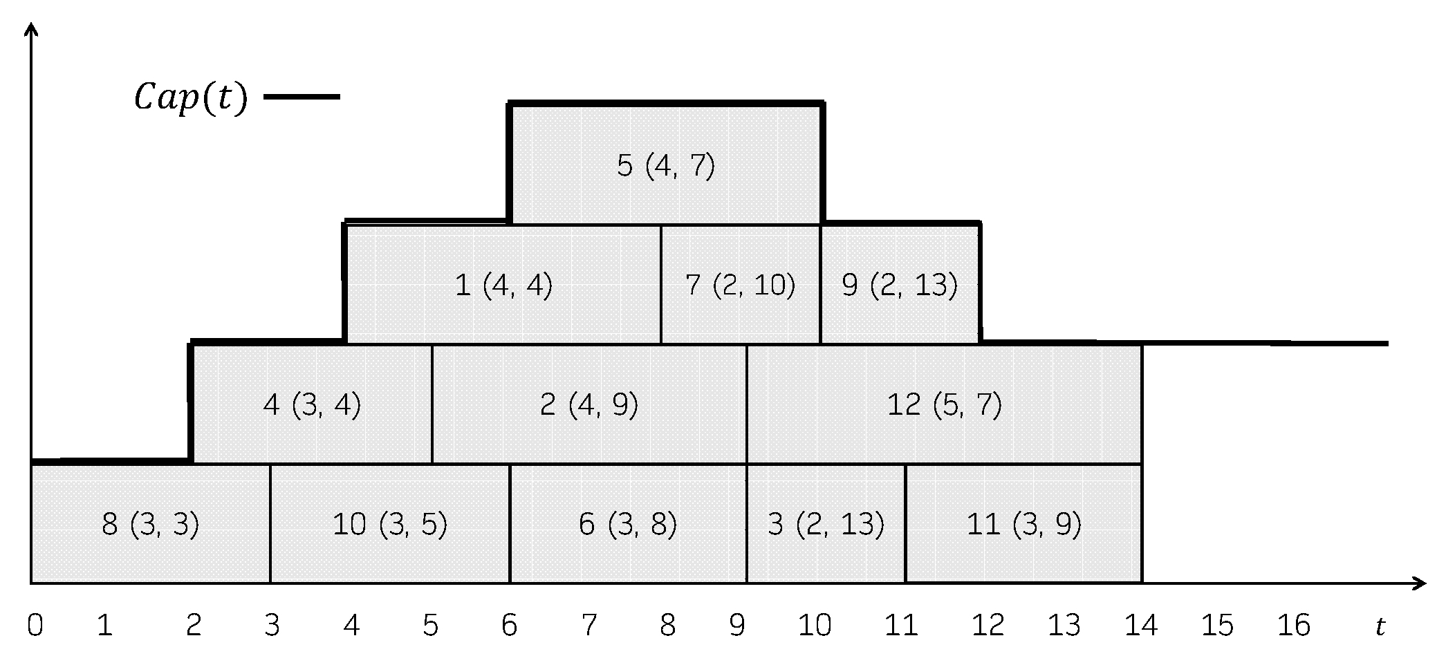
Figure 1 shows a feasible schedule. For each job, its processing time and its due date is represented in parentheses. The capacity of the machine over time, , is shown in the Gantt chart as well. The total consumption is not explicitly represented, but it can be easily seen that it always holds that . In this schedule, the jobs that incur in a positive tardiness are 1 (), 2 (), 4 (), 5 (), 6 () and 8 (). So, its total tardiness is 37. Figure 2 shows another feasible schedule. As can be seen, the consumption never exceeds the capacity of the machine, even though job 2 is represented above the capacity line in the Gantt chart. In this case, the jobs that incur in a positive tardiness are 1 (), 2 (), 4 (), 5 (), 6 () and 8 (). So, its total tardiness is 40.
This problem arose in the context of scheduling the charging times of a fleet of electric vehicles in a community park [29]. In this scenario, it appears as a subproblem of the Electric Vehicles Charging Scheduling Problem (EVCSP), which considers a station with three charging lines and power and balance constraints on their load. The problem focuses on scheduling the charging times of the vehicles in one line at a given point in time, subject to maximum load constraints, which result in the definition of for a given problem instance. In [29], was expected to be a unimodal step function, first growing until reaching a peak and then decreasing until getting stabilized at a value greater than 0. Nevertheless, the formal definition of the problem does not impose to be of any given form.
The problem was proven NP-hard [32] by reducing the and the problems to it. These problems are known to be NP-hard [36]. In the problem the machine has a constant capacity of one unit, whereas in the problem there are m identical parallel machines. Any instance of these problems can be reduced to the problem by simply defining the capacity of the machine as or for all , respectively.
3. Preliminaries
This section summarizes the main components of the memetic algorithm proposed in [32], namely, the schedule builder used to define the search space, the genetic algorithm, the local search procedure and their combination.
3.1. Schedule Builder
The definition of a suitable search space is an essential step in the development of effective scheduling algorithms. To this aim, schedule builders, or schedule generation schemes, have been commonly used (e.g., [37,38,39,40,41,42]). Schedule builders are non-deterministic constructive methods that allow the computation and enumeration of a subset of the feasible schedules, thus implicitly defining a search space.
Algorithm 1 shows the pseudocode of the schedule builder proposed in [31,32] for the problem. It maintains a set containing the jobs to be scheduled, which is initialized to the set of all jobs . The algorithm proceeds iteratively: at each iteration a job is selected (non-deterministically) and it is scheduled at the earliest possible time such that the capacity of the machine is not exceeded at any time. After scheduling the job u, the consumption of the machine is updated accordingly and u is removed from . The algorithm terminates when all the jobs have been scheduled, returning a feasible schedule.
Notice that the job to be scheduled at each iteration is selected non-deterministically. This way, the schedule computed depends on the sequence of choices made. For example, considering the problem instance in Example 1, the sequence of choices would result in the schedule shown in Figure 1. The sequence would lead the schedule builder to compute the same schedule, so this mapping is many-to-one.
Regardless of these choices, the schedule builder always returns a so-called left-shifted schedule, in which no job can be scheduled earlier without delaying the starting time of another job [43]. An example of such a schedule is the one shown in Figure 1. However, the schedule shown in Figure 2 is not left-shifted since, for instance, jobs 2, 5 or 6 could be moved to start earlier without delaying any other job.
| Algorithm 1 Schedule Builder ([31,32]) |
 |
In addition, the non-deterministic selection of jobs in Algorithm 1 enables the definition of a search space containing all left-shifted schedules, by considering all possible sequences of choices (i.e., permutations of the set of jobs). This search space is guaranteed to contain at least one optimal solution to any problem instance. For further details, the interested reader is referred to [32].
Among different possibilities, the schedule builder can be used in combination with a priority rule or as the decoder of a genetic algorithm, as described below.
3.2. Genetic Algorithm
Genetic algorithms (GAs) are population-based metaheuristics inspired by the theory of evolution [44]. GAs have been successful at solving combinatorial optimization problems, including scheduling problems (e.g., [11,14,45,46]).
Algorithm 2 depicts the main structure of the genetic algorithm proposed in [31,32] for solving the problem. The GA has four parameters: crossover and mutation probabilities ( and ), number of generations () and population size (). Initially, the first population is generated at random and evaluated. Then, at each generation, the population is evolved by the application of selection, recombination, evaluation and replacement operators. In the selection phase chromosomes are organized into pairs at random. Each of these pairs undergoes crossover and mutation operators with probabilities and , respectively, what results in two offspring. Then, the new individuals are evaluated, obtaining the actual solutions they represent. Finally, the new population is built in the replacement phase, by a process in which the parents and their offpring compete in a tournament. The GA terminates when generations have been completed, returning the best schedule found. However, other termination criteria could be used instead, as establishing a time limit.
Chromosomes in the GA are permutations of the set of job indices, defining total orderings among the jobs. The GA uses the well-known Order Crossover (OX) operator [47], by which an offspring inherits the positions of a (random) subset of the jobs from the first parent and the relative order of the remaining jobs from the second parent. As mutation operator, the GA uses a simple procedure that swaps two random elements in the chromosome. The evaluation of a chromosome is done by means of the schedule builder shown in Algorithm 1, scheduling the jobs in the order they appear in the chromosome. Specifically, given a chromosome , at the i-th iteration the schedule builder selects and schedules the job . This results in a feasible left-shifted schedule. For example, considering the problem instance in Example 1, the chromosome (3, 12, 10, 7, 1, 9, 11, 4, 8, 6, 2, 5) would lead to the schedule shown in Figure 1.
| Algorithm 2 Genetic Algorithm ([31,32]) |
 |
3.3. Local Search Procedure
Local search algorithms have been widely used for solving a variety of hard scheduling problems (e.g., [15,16,17]). These methods aim at iteratively improving the quality of a given solution by performing changes on it, moving to neighbouring solutions.
The local search procedure our contributions build on is based on swapping pairs of consecutive jobs in a feasible left-shifted schedule. Two jobs i and j are consecutive in a schedule S if or , i.e., if one of the jobs starts its processing just after the other one is completed.
As proven in [32], swapping a pair of consecutive jobs in a schedule S results in a new feasible schedule where all the other jobs keep their starting time (and so their tardiness). As a consequence, if the total tardiness of S is known in advance, the total tardiness of can be computed in constant time as , where and . This allows for establishing an efficient improvement condition of over S from swapping the pair of consecutive jobs : improves S if and only if .
The results above serve to define a neighbourhood structure, consisting of all the pairs of consecutive jobs in a given schedule. This structure could be exploited by any standard local search approach (e.g., simulated annealing [48], tabu search [49], etc.). However, as pointed out in [32], jobs with earlier starting times in a schedule could be expected to contribute less to the total tardiness than those that start their processing later. This observation led to the definition of an efficient local search procedure, aiming at delaying jobs with low tardiness values in favor of jobs with higher values.
The procedure exploits the notion of C-path, defined as a maximal sequence of pair-wise consecutive jobs in a feasible schedule. As an example, in the schedule shown in Figure 1, the sequence of jobs constitutes a C-path. Other examples are , and . This concept is similar to the notion of critical block commonly used in the context of shop scheduling problems [16,50]. Throughout, for a C-path P, will denote its tardiness, i.e., the sum of the tardiness values of all the jobs contained in it. In addition, will denote the k-th job in P, with k an integer index in the interval .
Algorithm 3 shows the local search approach (the pseudocode of the local search procedure proposed in [32] has been split in Algorithms 3 and 4 to improve the presentation of the new local search algorithms described in Section 4), referred to as Single C-path local search (SCP) herein. It is based on the observation that rearranging the jobs in a C-path P does not alter the tardiness of any job outside P. As can be observed, given a feasible left-shifted schedule S, SCP consists of two phases: it first computes a random C-path P in S, which is then processed in order to improve its tardiness. As a result a (potentially) improved feasible left-shifted schedule is returned, i.e., .
Computing an optimal order of the jobs in a C-path can be seen as an instance of the problem. This problem is known to be NP-hard [51], so solving it to optimality may be too time-consuming. As an alternative, SCP uses the efficient procedure , shown in Algorithm 4. This procedure operates on a feasible schedule and on a C-path , initialized as copies of the input schedule S and input C-path P. The algorithm traverses from left to right. At each iteration, it considers the job , and swaps it with the next job in the C-path while the aforementioned improvement condition is fulfilled. Upon termination, the algorithm returns and .
Notice that, although is deterministic, it operates on a random C-path, what introduces a source of randomness to the SCP procedure.
The procedure performs at most swap operations, what gives an upper bound on its runtime complexity, since both testing the improvement condition and swapping jobs can be done in constant time. As a result, the SCP local search procedure runs in , with n the number of jobs, as in the worst case .
| Algorithm 3 Single C-path local search (SCP) |
Data: A feasible schedule S. Result: A feasible schedule with . ; ; return ; |
| Algorithm 4 |
 |
3.4. Memetic Algorithm
Memetic algorithms (MAs) are hybrid metaheuristics that result from combining genetic algorithms and local search methods [52]. These algorithms are often able to keep a proper balance between the exploration and exploitation of the search space. The GA searches for solutions globally, guiding the process towards promising areas, whereas local search intensifies the search locally, what leads to finding better solutions. As a result, MAs have been very effective at solving scheduling problems (e.g., [18,19,53,54,55]).
The memetic algorithm proposed in [32] for the problem has the same structure as the GA shown in Algorithm 2. However, after a feasible schedule is computed by the schedule builder (Algorithm 1) in the evaluation phase, the MA uses the SCP local search procedure (Algorithm 3) in an attempt to improve it.
In order to incorporate the characteristics of the improved schedules into the population, the MA implements a Lamarackian evolution model by which the improved schedule is coded back into the chromosome it came from. This is done by replacing the chromosome by a new one where the jobs in the C-path P processed by the SCP procedure appear in same order as in the resulting C-path , and all the other jobs keep the same positions. This way, the new chromosome would lead the schedule builder to build the improved schedule .
Throughout, this memetic algorithm will be referred to as MA.
4. New Local Search Procedures
This section describes the proposed new local search procedures for the problem. The new methods build on the SCP local search algorithm described in Section 3.3. These are aimed at making the local search more effective and, at the same time, keeping their complexity low.
4.1. Enhancements to Single C-Path Local Search
First, two enhancements to the SCP procedure are proposed, both operating on a single C-path. The first one extends the condition for swapping two consecutive jobs, whereas the second one integrates a hill climbing approach for improving a C-path to a greater extent.
4.1.1. Slack-Aware Improvement Condition
The SCP procedure swaps two consecutive jobs in a C-path if the improvement condition holds. This way, performing a swap operation always results in a feasible schedule with less total tardiness. However, there may be situations where the condition is not fulfilled, but swapping the jobs may still be beneficial.
Consider the case that , i.e., swapping the jobs would not have any (immediate) effect in the total tardiness of the resulting schedule. Since the C-path is processed from left to right, further improvements would be more likely to occur in subsequent iterations if the job that is left in the second place had a greater slack, defined as the difference between its due date and its completion time. Notice that a positive slack means that the job would be completed before its deadline, whereas a negative slack indicates that the job would incur in some (positive) tardiness.
This way, if the jobs i and j are not swapped, the job left in the second position would be j, and its slack would be . On the other hand, if the jobs are swapped, the second job would be i, with a slack of , where . Since it suffices to compare the due dates of the jobs to determine whether . This results in the extended improvement condition shown in the following equation:
Example 2.
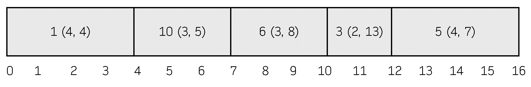
Consider the schedule depicted in Figure 1, and the C-path (3, 10, 1, 6, 5). If the procedure is run with the original improvement condition, no swap operation would be performed. However, the use of the slack-aware condition results in several swaps, leading to reductions in the total tardiness along the process. The resulting C-path is shown in Figure 3, with a total tardiness of 13, given by the jobs 10 (), 6 () and 5 (). The resulting schedule has a total tardiness of 32, five units less than the original one.
By using the slack-aware improvement condition, there is the guarantee that the final schedule will be such that , since no swap operation that increases the total tardiness is ever performed. In addition, the new condition does not affect the worst-case complexity of the method, as it can be checked in constant time and the maximum possible number of swap operations remains the same.
Throughout, the predicate will indicate whether the improvement condition holds for a pair of consecutive jobs . Besides, the SCP procedure using the new improvement condition will be referred to as iSCP.
4.1.2. Hill Climbing on a Single C-Path
An analysis of the procedure (Algorithm 4) reveals that the resulting C-path may be further improved by swapping some pair of consecutive jobs.
Suppose that in a given iteration there are three consecutive jobs in the C-path P, i.e., , and that the improvement condition does not hold. This way, the jobs i and j are not swapped and, by construction of the algorithm, i will not be swapped with any other job that appears after it. If in the next iteration the algorithm swaps j and k, the final C-path will be of the form , since j and k could be swapped with other jobs in subsequent iterations. In this situation, swapping i with the next job in the C-path might result in an improvement.
Example 3.
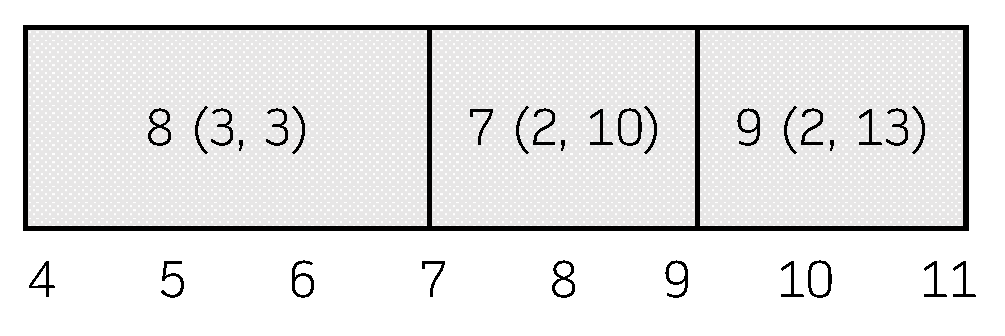
Consider the schedule depicted in Figure 1, and the C-path (7, 9, 8). In the first iteration, the procedure (using the slack-aware improvement condition) does not swap the jobs 7 and 9. In the second iteration, it swaps the jobs 9 and 8, what results in the C-path (7, 8, 9). Now, if this procedure is issued again, the jobs 7 and 8 would be swapped and the final C-path would be (8, 7, 9), shown in Figure 4. The new C-path has a total tardiness of 4, given by job 8 (), four units less than the original one.
The observation above serves to develop an improved version of , by performing a hill-climbing approach. The new version of the method, termed , is shown in Algorithm 5. As can be observed, the method repeatedly invokes until there are no reductions in the total tardiness objective function. Upon termination, the method reaches a fixpoint where swapping any pair of consecutive jobs in the C-path does not result in an improvement. As can be observed, the structure of is similar to the Bubble Sort algorithm: each invocation to the procedure could be related to one pass of the sorting algorithm, and it terminates when no swaps are made in a given iteration.
Noticeably, given a schedule S and a C-path P in S as input, the procedure performs at most iterations.
To show this, it is first proven that after the i-th iteration, the last i jobs in the C-path become fixed, i.e., they will not be rearranged in any future iterations of the method. This follows from the next result:
Lemma 1.
Let P be the initial C-path, L = and , with , the C-path computed after the i-th iteration of . Then, for all .
Proof.
The lemma is proven by induction on the number of iterations.
(Base case: ) only if at some step in the computation of there are two consecutive jobs such that the condition does not hold and with . Suppose, w.l.o.g., that there is only one such pair of consecutive jobs. Since does not hold, will not be swapped with in the computation of . So, .
(Inductive step: ) Assume as inductive hypothesis that for all . only if at some step in the computation of there are two consecutive jobs such that the condition does not hold and , with . Suppose, w.l.o.g., that there is only one such pair of consecutive jobs. As the inductive hypothesis holds, it must be that does not hold for any . So, . Since does not hold, will not be swapped with in the computation of . Hence, and hence for all . □
Now, the bound on the maximum number of iterations performed by can be easily shown.
Proposition 1.
performs at most iterations.
Proof.
By Lemma 1, after the -th iteration, it holds that for all . Since there is only one job left (the first one), it must also hold that . So, in the -th iteration no swaps are made, what results in the termination of . □
Interestingly, the procedure exhibits the same worst-case complexity than , as shown next:
Proposition 2.
runs in .
Proof.
Note that if two consecutive jobs i and j are swapped, they will not be swapped in subsequent iterations, since the improvement condition would not hold in the opposite direction. In P there are possible unordered pairs of jobs, what gives an upper bound of the total number of swap operations that the algorithm can possibly perform along its execution. Now, let denote the number of swap operations performed at the i-th iteration. Since the whole C-path is traversed, this results in checks of the improvement condition. By Proposition 1, there can be at most iterations. Hence, the total number of checks will be . Since both performing a swap operation and testing the improvement condition are done in constant time, the complexity of is . □
The use of gives rise to a new local search method, termed SCP+, that is shown in Algorithm 6. As SCP, the new method computes a random C-path P and tries to improve it. However, in the second phase it invokes instead of the simpler . In the worst case , with , so SCP+ runs in .
| Algorithm 5 |
 |
| Algorithm 6 SCP with Hill Climbing (SCP+) |
Data: A feasible schedule S. Result: A feasible schedule with . ; ; return ; |
4.2. Cover-Based Local Search
The previous methods aim at improving a single C-path P in a schedule, leaving all the jobs outside P unaltered. Clearly, processing these jobs could bring additional improvements.
This section proposes a new procedure based on computing and processing a cover of C-paths, that is, a set of C-paths such that the union of their elements hits all the jobs in . In order to be able to efficiently process the C-paths independently from each other, the cover is restricted to be a partition of the set . This way, given a schedule S a cover is a set of maximal sequences of pair-wise consecutive jobs in S, such that each job in belongs to exactly one . Notice that such sequences may not be maximal w.r.t. all the jobs in S. Anyway, each in the cover will be maximal w.r.t. the jobs that do not belong to any other , with . So, slightly abusing notation, it is referred to as a C-path.
Once a cover is computed, the new cover-based local search procedure, termed CB, processes each of the C-paths, aiming at reducing their total tardiness.
Example 4.
Consider the schedule shown in Figure 1. The first step taken by CB is computing a cover of C-paths, for instance , with , , and . Then, the procedure is invoked on each C-path in the cover, what results in the improved C-paths , , and . Note that since there is only one job in no improvements are possible. After all the C-paths have bee processed, the resulting schedule, shown in Figure 5 has a total tardiness of 25, twelve units less than the original one.
The computation of a cover of C-paths is depicted in Algorithm 7. The algorithm operates on a list R of jobs and maintains a set of sequences of pair-wise consecutive jobs. is initialized as the empty set and will eventually contain the cover of C-paths returned by the method. The list R contains the jobs sorted non-decreasingly by their starting times in the schedule S given as input. Then, R is traversed from left to right. At the i-th iteration, the method looks for a sequence to append the job , i.e., such that its last job is completed exactly at the starting time of . To this aim, it uses the function , that returns the index of in if such sequence exists and the value 0 otherwise. If a sequence is found, the job is appended at its end. Otherwise a new sequence is created and added to .
It is easy to see that computing a cover of C-paths is done in . First, the complexity of sorting the jobs is , e.g., by using the algorithm [56]. Second, the loop iterates over all the n jobs, and for each job it may have to traverse the whole set , what gives the complexity .
| Algorithm 7 |
 |
Algorithm 8 shows the pseudocode of the cover-based local search procedure. As can be observed, it first computes a cover of C-paths by using Algorithm 7. Then, the method attempts to improve each C-path in the cover by means of the procedure . Notice that processing does not interfere with any other C-paths, since in every job belongs to only one C-path. Finally, the improved schedule is returned.
| Algorithm 8 Cover-based Local Search Procedure (CB) |
 |
As invoking never increases the total tardiness, it follows that . Besides, as the previous methods, the new local search procedure has a worst-case quadratic complexity, as shown next:
Proposition 3.
CB runs in .
Proof.
Computing the cover of C-paths in the first phase is done in . Then, in the second phase the method performs k iterations. At the i-th iteration, by Proposition 2, invoking on has a complexity of . Notice that . Since , the runtime complexity of the loop is bounded by . So, CB runs in . □
4.3. Interchanging Jobs between C-Paths
The CB procedure processes the C-paths in a cover independently from each other, aiming at reducing their total tardiness. As an alternative, the global quality of the schedule could be improved by swapping jobs that belong to different C-paths.
Let S be a feasible schedule, and two C-paths in a cover, and consider the jobs and such that . The jobs i and j can be interchanged without interfering with any other C-paths if the following capacity condition holds in S: just after the completion of the last job in there are at least time instants t where . In this situation, interchanging the jobs results in a new schedule where and . In addition, all the jobs in after i are delayed time units (thus potentially increasing their tardiness), and the jobs in after j are scheduled time units earlier (potentially reducing their tardiness), guaranteeing that is a left-shifted schedule.
If the new C-paths and are such that , would have a higher quality than S in terms of total tardiness.
Example 5.
Consider the schedule from Example 4 depicted in Figure 5, and the cover of C-paths , with , , and . The jobs 1 (in ) and 8 (in ) can be interchanged, as the capacity condition is fulfilled, and this operation results in a feasible schedule with less total tardiness. The same applies to the jobs 5 (in ) and 11 (in ). As a consequence, the resulting schedule, depicted in Figure 6, has a total tardiness of 22, three units less than the original one.
Building on the previous idea, Algorithm 9 shows a new local search procedure, termed ICP, that attempts to reduce the total tardiness of a schedule S by means of interchanging jobs between C-paths. First, a cover of C-paths is computed using Algorithm 7. At this point, the algorithm proceeds iteratively. It operates over a feasible schedule , initialized as a copy of S. At each iteration, the C-path with the greatest tardiness is selected. Then, the algorithm traverses all the C-paths different from , and for each job in and each job in , it tests whether interchanging them is possible (i.e., if the aforementioned capacity condition holds). If so, the jobs are interchanged resulting in the new left-shifted schedule . This operation is performed by the procedure , which delays and moves earlier the jobs in the C-paths after and if necessary. If , is replaced by . Finally, is removed from and a new iteration is performed. The method terminates when , returning the (possibly) improved schedule .
| Algorithm 9 Local search by interchanging jobs between C-paths (ICP) |
 |
By construction, in the worst case, the ICP procedure will interchange pairs of jobs. On the other hand, the necessary operations for interchanging two jobs result in a linear overhead. Hence, the complexity of ICP is bounded by .
4.4. Hybrid Approach
In order to benefit from all the methods described above, this section proposes a hybrid approach, termed HYB, that combines the CB and the ICP procedures.
Given a feasible schedule S as input, the new method works as follows: first a cover of C-paths is computed and, as CB does, each is processed by means of the procedure, resulting in the improved C-path . This produces a (potentially) better schedule , and the cover . Then, the schedule undergoes the loop of ICP, by which jobs are interchanged between different C-paths in the cover .
By the properties of CB and ICP, the final schedule will never have a greater total tardiness than that of the original one. Furthermore, the complexity of HYB is bounded by , given by the ICP component of the method.
5. New Memetic Algorithms
The efficiency of the local search methods proposed in the previous section makes them well-suited for working in combination with the genetic algorithm described in Section 3.2, each of them giving rise to a different memetic algorithm.
The new algorithms have the same structure as the MA proposed in [32] (described in Section 3.4), only differing in the local search procedure used. After a schedule is computed by the schedule builder (Algorithm 1) in the evaluation phase of the GA, a local search procedure is issued with the aim of improving it.
As a consequence, five new memetic algorithms for the problem are proposed: MA, MA, MA, MA and MA. MA uses the SCP procedure (Algorithm 3) with the slack-aware improvement condition proposed in Section 4.1.1. MA combines the GA with the hill-climbing approach SCP+ (Algorithm 6) described in Section 4.1.2. MA integrates the cover-based local search method CB (Algorithm 8) introduced in Section 4.2. MA uses the local search procedure ICP (Algorithm 9), based on interchanging jobs between C-paths as described in Section 4.3. Finally, MA exploits the hybrid local search procedure presented in Section 4.4.
As the MA proposed in [32], the new memetic algorithms instrument a Lamarckian evolution model, by which the characteristics of the improved schedules are transmitted to the population. This is done by a simple procedure that swaps two job indices in the chromosomes whenever the local search methods swap or interchange a pair of jobs. This way, the improved schedules are coded back into the chromosomes, what facilitates that the MAs converge to high-quality solutions. Notice that running the schedule builder on the resulting chromosomes would result in the improved schedules computed by the local search methods.
The complexity of the memetic algorithms depends on the population size (), the number of generations () and the complexity of the local search method used. Since the complexity of the genetic operators is not greater than that of the local search procedures, the complexity of MA, MA and MA is given by , whereas MA and MA have a complexity of ).
6. Results
This section reports the results from an experimental study carried out to assess the performance of the algorithms proposed in this paper.
The experiments were carried out over a set of instances built for this purpose, using the random generation procedure proposed in [35]. Given a number of jobs (n) and the maximum capacity of the machine (), the generator produces instances where is an unimodal step function, making them similar in structure to those expected to arise in the context of electric vehicles charging [29].
The generation procedure works as follows ( denotes a random integer from a uniform distribution in , and denotes a random integer from a normal distribution with mean and standard deviation ): First, each job i is assigned a processing time , and and are defined. The initial capacity of the machine is , and its final capacity is . Then, is defined by means of different capacity intervals, first increasing the capacity in one unit from to , and then reducing it one by one until reaching . Each interval has a duration of , with , and . This seeks that the jobs are distributed over all the capacity intervals. Finally, each job i is assigned a due date , where is an approximation of completion time of all the jobs.
Using the approach above, 10 instances with each of the following configurations of n and were generated: and ; and ; and ; and and and . In all, the benchmark set consists of 190 instances. Note that earlier work [32] considered instances with up to 120 jobs in the experimental study. Herein, most of the instances are (much) larger, and so (much) more challenging what serves to evaluate how the different methods scale in practice.
A prototype was coded in C++ and all the experiments were run on a Linux cluster (Intel Xeon 2.26 GHz. 128 GB RAM).
To assess the performance of the proposed methods six memetic algorithms are compared, termed MA, MA, MA, MA, MA and MA. Recall that MA is the memetic algorithm proposed in [32], whereas the other MAs are the new ones proposed in this work, described in Section 5.
For each instance, 30 independent runs of each method were performed, recording the best and average total tardiness of the solutions found. Following [32], the considered MAs were run with a population size of 250 individuals, and crossover and mutation probabilities of 0.9 and 0.1, respectively. In addition, to make the comparison fair, the termination condition is a given time limit, which was set depending on the size of the instances. Specifically, for an instance with n jobs, the time limit is set to s, which in most cases is sufficient for the algorithms to converge and, arguably, it constitutes a reasonable time in practice given the complexity of the problem.
In order to evaluate the quality of the solutions, the error in percentage w.r.t. the best solution found across all the experiments is calculated for the solutions reached by each method on each instance. Specifically, if for a given instance the best known solution has a total tardiness and an algorithm finds a solution with a total tardiness T (with ), the error in percentage is computed as . This way, the error in percentage of a solution represents its deviation from the best solution known for a given problem instance.
The experimental study is organized as follows: First, the slack-aware improvement condition is analyzed by comparing MA and MA. Then, the performance of the memetic algorithms MA, MA, MA and MA is assessed. Finally, the study provides a detailed comparison of the best memetic algorithm with both the state-of-the-art approach [32] and a constraint programming model.
6.1. Analyzing the Slack-Aware Improvement Condition
The objective of the first series of experiments is to measure the effectiveness of the slack-aware improvement condition described in Section 4.1.1, and assess the gains it brings in terms of the quality of the schedules computed. To this end, MA and MA were run on all the instances. Recall that MA exploits the SCP local search procedure using the original improvement condition for swapping a pair of consecutive jobs in a C-path, whereas MA integrates the iSCP procedure, which uses the new slack-aware condition.
Table 1 shows a summary of the results. For each method, it reports the error in percentage of the best and average solutions, averaged for groups of instances with the same size n and maximum capacity of the machine . As can be observed, MA yields (much) better results than MA on all the groups of instances, in both the best and average solutions found. The improvements in the quality of the solutions are significant. On average, the error of the best and average solutions computed by MA is about and of that of the solutions found by MA. The greatest improvements are observed for the instances with , where the ratios are and . On the other hand, the results show that the errors tend to increase with . This is always the case for MA, whereas MA follows this trend for most values, with the exception of for .
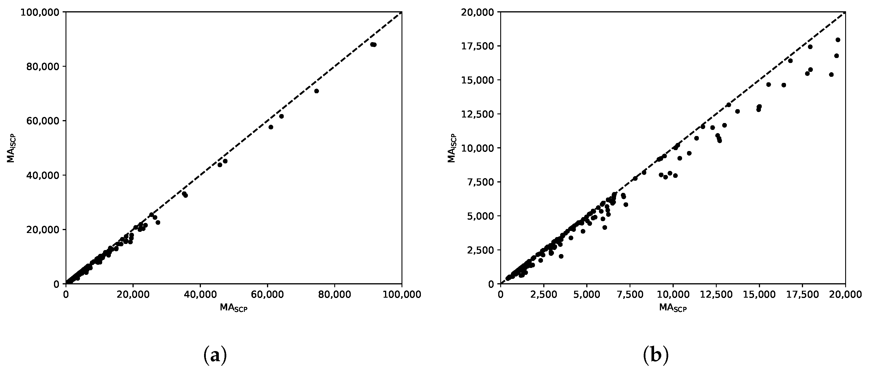
Figure 7 shows two scatter plots with the average total tardiness of the solutions computed by the methods. Notice that the plots show total tardiness values, instead of errors in percentage as reported in Table 1. Figure 7a shows these values for all the instances (notice that the axes are limited to 100,000) and, to get a closer view, Figure 7b shows the values below 20,000, which contains most of the instances (with the exception of a few outliers). In these plots, the points below (resp. above) the diagonal line represent instances for which MA returned better (resp. worse) solutions on average than MA. As can be observed, there is a clear superiority of MA over MA.
The results confirm that the slack-aware improvement condition is beneficial. As a consequence, this condition will be used in all the memetic algorithms evaluated in the next subsection.
6.2. Analyzing MA, MA, MA and MA
The second part of the experimental study is devoted to the evaluation of the memetic algorithms MA, MA, MA and MA, which use the local search procedures SCP+, CB, ICP and HYB respectively.
As in the previous experiments, 30 independent runs of the methods were performed on each instance in the benchmark set. The results are summarized in Table 2. As can be observed, on average all the algorithms improve the results obtained by MA and MA (shown in Table 1), some of them very substantially. For most groups of instances the hill-climbing approach used by SCP+ leads to solutions of similar quality than those computed by MA, with the notable exception of the largest (and hardest) instances with , where the errors are much smaller. MA reaches significantly better solutions than MA in all cases, indicating a remarkable effectiveness of the cover-based local search method. On the other hand, MA lays behind all the other memetic algorithms in the table, what suggests that the ICP procedure is not as effective as the other local search methods. However, the combination of CB and ICP is beneficial in practice, as it allows MA to achieve the best results by a wide margin. In most cases, both the best and average solutions computed by MA have an error between and , and the average error of the solutions computed by MA is smaller than that of the best solutions computed by any other method.
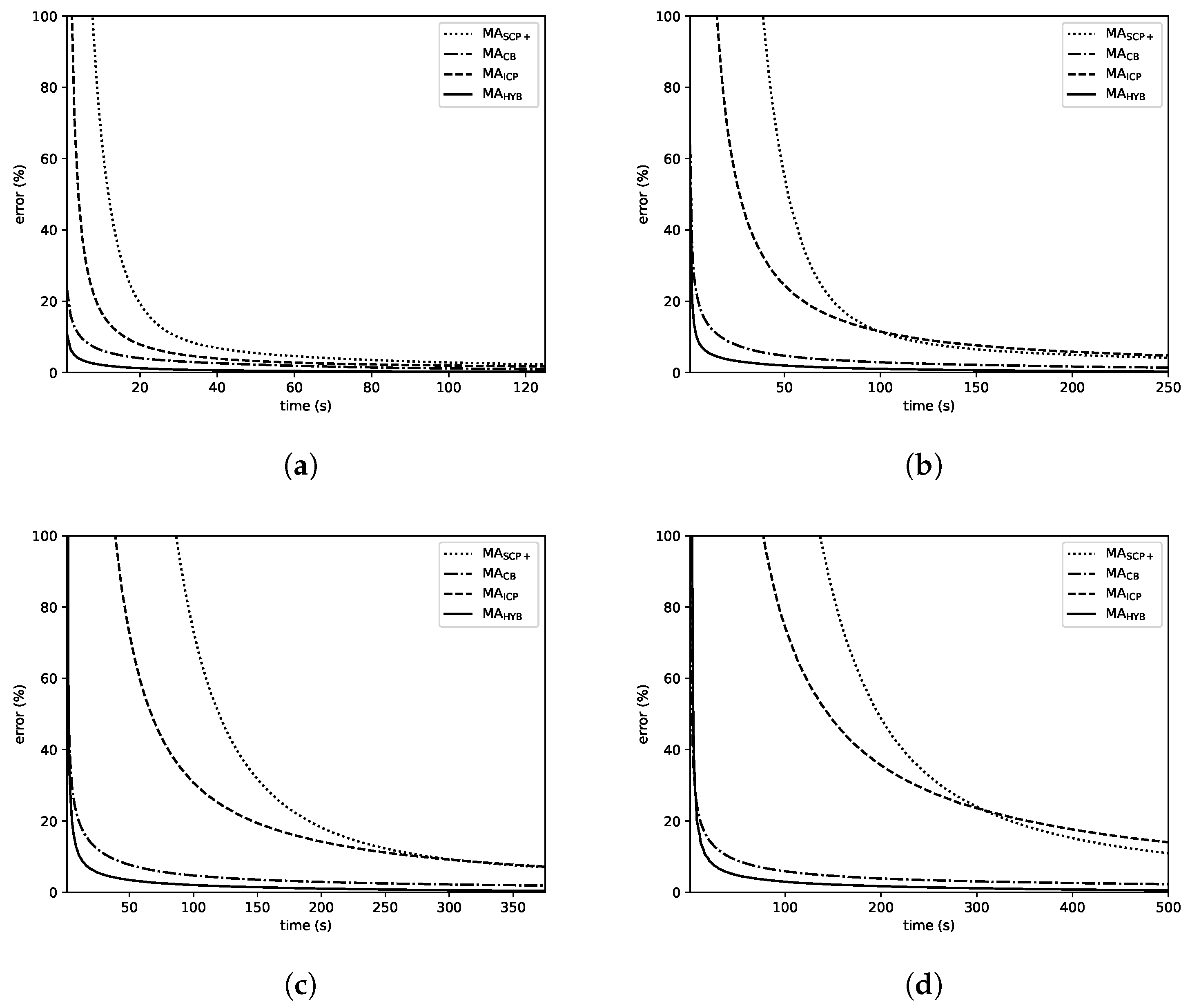
Figure 8 shows the evolution over time of the average error of the solutions computed the memetic algorithms on the sets of instances with 250, 500, 750 and 1000 jobs. Although the errors in the plots are different, there are similarities shared by all of them. First of all, it is clear that MA and MA are in the first and second positions from the beginning for all the considered sizes, and these methods keep their lead for the whole duration of the experiments. In addition, MA exhibits a faster convergence pattern than MA, allowing it to compute better solutions during a large fraction of the given time. However MA is eventually able to compute solutions of similar quality and even outperform MA on the largest instances. Noticeably, the differences in favor of MA and MA over the other algorithms grow with n. In the case of , all the MAs are close, even though the mentioned ranking among them is already observable; with and , the superiority of MA and MA becomes clearer and finally, with , it is evident. In addition, these two algorithms (especially MA) are able to compute high-quality solutions in short time (using just a small portion of the given time limit), what represents an important advantage over the other methods.
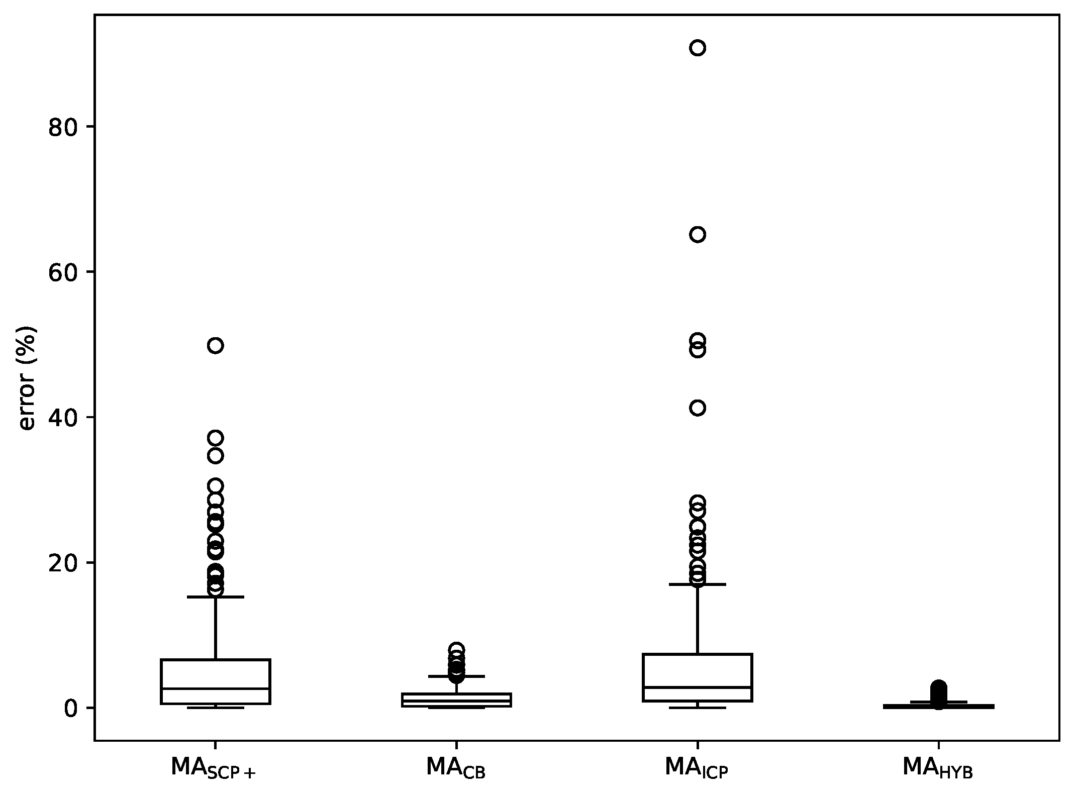
Figure 9 shows a boxplot with the average errors of MA, MA, MA and MA over the whole set of instances. It confirms the previously made points: MA is ahead in terms of results, followed by MA, MA and MA.
Some conclusions can be drawn from the experiments. First of all, the cover-based methods get the best results, since MA and MA are ahead of the other approaches in terms of the quality of solutions they reach. In addition, as already mentioned, ICP does not seem to be a good stand-alone local search for a memetic algorithm considering that MA is outperformed by every other method in this comparison; however, its combination with CB in MA leads to the best overall results, so, all things considered, it is a useful technique.
6.3. Final Comparison
The experimental study concludes comparing the best memetic algorithm among the ones proposed in this paper (MA) and two other methods, namely, the memetic algorithm MA proposed in [32] and a constraint programming approach.
To our best knowledge, MA is the current best-performing approach in the literature. As pointed out, this method was shown to outperform the genetic algorithm previously proposed in [31], as well as priority rules, both classical ones and others built by means of genetic programming approaches [34,35] in terms of the quality of the solutions computed.
In order to make the comparison more comprehensive, MA is also compared to a constraint programming approach that was built using the commercial solver IBM ILOG CP Optimizer (version 12.9). This solver is specialized in scheduling and has been shown to be very effective in different problems [9,57]. The problem was modeled in a conventional way, using interval variables (IloIntervalVar) to represent the jobs. The machine was modeled as a non-renewable resource using a cumulative function defined as a sum of pulse functions (IloPulse), enforcing that its capacity is never exceeded by an IloAlwaysIn constraint for each capacity interval. Finally, the objective function was set to minimize the total tardiness, defined as a numerical expression (IloNumExpr) that sums the positive differences between the completion time of the jobs and their due dates.
The constraint programming approach, referred to as CPO, was implemented in C++. Besides, 30 independent runs were performed on each instance (since it has some stochasticity), setting a time limit of s, as for the other methods. In all these experiments, CPO was run using one worker and the default values for CP Optimizer’s parameters.
Table 3 shows the results obtained by MA, CPO and MA in terms of the error of the solutions reached by each algorithm. As can be observed, MA conclusively outperforms MA and CPO. For all groups of instances, the errors yielded by MA are at least one order of magnitude smaller than the errors of the solutions computed by the two other methods. MA performs (much) better than CPO on the smaller instances with , whereas for the largest instances CPO gets better results. This suggests that MA suffers from some scalability issues, what indicates that the SCP local search method becomes less effective as the size of the instances grows. However, the new local search methods proposed in this paper lead MA to scale to much larger instances, always finding solutions very close to the best known ones.
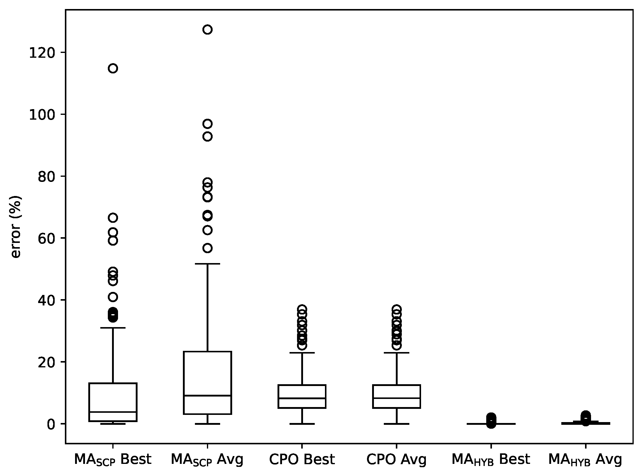
Figure 10 depicts a boxplot with the best and average errors of the three methods over the whole set of instances. It confirms that MA is clearly outperforms both MA and CPO, with no overlapping between its boxes and those of the other two methods. In addition, the plot shows that even the few outliers from MA correspond to solutions with small errors.
A series of statistical inference tests was performed to the results shown in Table 3 with the objective of making the experimental study more robust. The tests are aimed at the detection of statistically significant differences among the average errors of the solutions yielded by the methods, and they were conducted over all the instances in the benchmark set.
In order to know if there are significant differences between the results achieved by the algorithms and rank them, an Aligned Friedman Rank Test was performed, following [46,58,59]. This is a multiple-comparison non-parametric test, whose null hypothesis considers that there are no differences in the rankings of the algorithms. If the null hypothesis is rejected, the method at the top of the ranking will be compared against the rest of them by means of a collection of post-hoc procedures. The considered post-hoc procedures (Bonferroni–Dunn, Holm, Hochberg, Hommel, Holland, Rom, Finn, Finner and Li) are described in [58].
The average ranking calculated by the Aligned Friedman Rank Test (distributed according to with 2 degrees of freedom: 135.68) is shown in Table 4. As can be observed, MA appears in first place, followed by CPO and MA in second and third place, respectively. The test returned a p-value of , meaning that the differences among the results yielded by the algorithms are statistically significant.
In order to compare MA with the other methods (MA and CPO), a series of post-hoc procedures were carried out. These procedures share the same null hypothesis, which states that the distributions of the results obtained by MA and the comparing methods are equal. Table 5 shows the adjusted p-values obtained by each procedure, (Bonferroni–Dunn), (Holm), (Hochberg), (Hommel), (Holland), (Rom), (Finner) and (Li). The results lead to the conclusion that the differences in favor of MA are statistically significant, since all the p-values are very close to 0, rejecting the null hypothesis in all cases.
7. Conclusions
The new local search methods developed in this paper have been shown to give rise to very effective memetic algorithms for solving the problem. The results from the experimental study confirm that each of the local search techniques brings improvements to the memetic algorithms in practice. MA, which exploits the hybrid local search procedure, stands out as the best method overall, computing high-quality solutions in short time and showing a remarkable ability to scale to large and challenging problem instances. As a result, this algorithm clearly outperforms existing approaches, including the memetic algorithm proposed in [32] and a constraint programming approach.
Although the memetic algorithms proposed in this paper are able to converge in short time, they may not be fast enough if real-time requirements are considered. However, the low worst-case complexities of the new local search procedures encourages further research in this direction, as deploying these methods in online settings. Future work will investigate their application in combination with real-time approaches, as schedule builders guided by priority rules. Hopefully, the local search procedures will be able to improve the quality of the solutions obtained by priority rules. In addition, another interesting topic for future research would be exploring the use of mathematical programming methods for solving the problem, as well as their combination with the algorithms proposed in this paper.
Author Contributions
Conceptualization, R.M. and C.M.; methodology, R.M and C.M.; software, R.M.; validation, R.M. and C.M; formal analysis, R.M. and C.M.; investigation, R.M. and C.M.; writing—original draft preparation, R.M. and C.M.; writing—review and editing, R.M. and C.M. All authors have read and agreed to the published version of the manuscript.
Funding
This research was supported by the Spanish Government under grant PID2019-106263RB-I00.
Institutional Review Board Statement
Not applicable.
Informed Consent Statement
Not applicable.
Data Availability Statement
The problem instances used in the experimental study and detailed results are available at https://github.com/raulmencia/One-Machine-Scheduling-with-Time-Dependent-Capacity-via-Efficient-Memetic-Algorithms.git (accessed on 19 November 2021).
Conflicts of Interest
The authors declare no conflict of interest.
References
- Pinedo, M.L. Planning and Scheduling in Manufacturing and Services; Springer: New York, NY, USA, 2009. [Google Scholar] [CrossRef]
- Zhan, Z.H.; Liu, X.F.; Gong, Y.J.; Zhang, J.; Chung, H.S.H.; Li, Y. Cloud Computing Resource Scheduling and a Survey of Its Evolutionary Approaches. ACM Comput. Surv. 2015, 47, 1–33. [Google Scholar] [CrossRef] [Green Version]
- Garey, M.R.; Johnson, D.S. Computers and Intractability; A Guide to the Theory of NP-Completeness; W. H. Freeman & Co.: New York, NY, USA, 1979. [Google Scholar]
- Brucker, P. Scheduling Algorithms, 4th ed.; Springer: Berlin/Heidelberg, Germany, 2004. [Google Scholar]
- Ganian, R.; Hamm, T.; Mescoff, G. The Complexity Landscape of Resource-Constrained Scheduling. In Proceedings of the Twenty-Ninth International Joint Conference on Artificial Intelligence, IJCAI 2020, Yokohama, Japan, 7–15 January 2021; IJCAI: Los Angeles, CA, USA, 2021; pp. 1741–1747. [Google Scholar] [CrossRef]
- Knust, S.; Brucker, P. Complexity Results for Scheduling Problems. Available online: http://www.informatik.uni-osnabrueck.de/knust/class/ (accessed on 19 November 2021).
- Carlier, J. The one-machine sequencing problem. Eur. J. Oper. Res. 1982, 11, 42–47. [Google Scholar] [CrossRef]
- Brucker, P.; Jurisch, B.; Sievers, B. A Branch and Bound Algorithm for the Job-Shop Scheduling Problem. Discret. Appl. Math. 1994, 49, 107–127. [Google Scholar] [CrossRef] [Green Version]
- Laborie, P.; Rogerie, J.; Shaw, P.; Vilím, P. IBM ILOG CP optimizer for scheduling - 20+ years of scheduling with constraints at IBM/ILOG. Constraints Int. J. 2018, 23, 210–250. [Google Scholar] [CrossRef]
- Ku, W.; Beck, J.C. Mixed Integer Programming models for job shop scheduling: A computational analysis. Comput. Oper. Res. 2016, 73, 165–173. [Google Scholar] [CrossRef] [Green Version]
- Mustu, S.; Eren, T. The single machine scheduling problem with sequence-dependent setup times and a learning effect on processing times. Appl. Soft Comput. 2018, 71, 291–306. [Google Scholar] [CrossRef]
- Soares, L.C.R.; Carvalho, M.A.M. Biased random-key genetic algorithm for scheduling identical parallel machines with tooling constraints. Eur. J. Oper. Res. 2020, 285, 955–964. [Google Scholar] [CrossRef]
- Gonçalves, J.F.; Resende, M.G.C. An extended Akers graphical method with a biased random-key genetic algorithm for job-shop scheduling. Int. Trans. Oper. Res. 2014, 21, 215–246. [Google Scholar] [CrossRef] [Green Version]
- Gonçalves, J.; Mendes, J.; Resende, M. A genetic algorithm for the resource constrained multi-project scheduling problem. Eur. J. Oper. Res. 2008, 189, 1171–1190. [Google Scholar] [CrossRef] [Green Version]
- Queiroga, E.; Pinheiro, R.G.S.; Christ, Q.; Subramanian, A.; Pessoa, A.A. Iterated local search for single machine total weighted tardiness batch scheduling. J. Heuristics 2021, 27, 353–438. [Google Scholar] [CrossRef]
- Nowicki, E.; Smutnicki, C. An Advanced Tabu Search Algorithm for the Job Shop Problem. J. Sched. 2005, 8, 145–159. [Google Scholar] [CrossRef]
- Chen, Y.; Lu, J.; He, R.; Ou, J. An Efficient Local Search Heuristic for Earth Observation Satellite Integrated Scheduling. Appl. Sci. 2020, 10, 5616. [Google Scholar] [CrossRef]
- França, P.M.; Mendes, A.; Moscato, P. A memetic algorithm for the total tardiness single machine scheduling problem. Eur. J. Oper. Res. 2001, 132, 224–242. [Google Scholar] [CrossRef]
- Abdel-Basset, M.; Mohamed, R.; Abouhawwash, M.; Chakrabortty, R.K.; Ryan, M.J. A Simple and Effective Approach for Tackling the Permutation Flow Shop Scheduling Problem. Mathematics 2021, 9, 270. [Google Scholar] [CrossRef]
- Onwubolu, G.; Davendra, D. Scheduling flow shops using differential evolution algorithm. Eur. J. Oper. Res. 2006, 171, 674–692. [Google Scholar] [CrossRef]
- Merkle, D.; Middendorf, M.; Schmeck, H. Ant colony optimization for resource-constrained project scheduling. IEEE Trans. Evol. Comput. 2002, 6, 333–346. [Google Scholar] [CrossRef] [Green Version]
- Zhou, H.; Pang, J.; Chen, P.K.; Chou, F.D. A modified particle swarm optimization algorithm for a batch-processing machine scheduling problem with arbitrary release times and non-identical job sizes. Comput. Ind. Eng. 2018, 123, 67–81. [Google Scholar] [CrossRef]
- Malakar, S.; Ghosh, M.; Bhowmik, S.; Sarkar, R.; Nasipuri, M. A GA based hierarchical feature selection approach for handwritten word recognition. Neural Comput. Appl. 2020, 32, 2533–2552. [Google Scholar] [CrossRef]
- Bacanin, N.; Stoean, R.; Zivkovic, M.; Petrovic, A.; Rashid, T.A.; Bezdan, T. Performance of a Novel Chaotic Firefly Algorithm with Enhanced Exploration for Tackling Global Optimization Problems: Application for Dropout Regularization. Mathematics 2021, 9, 2705. [Google Scholar] [CrossRef]
- Hall, N.G.; Potts, C.N. Supply Chain Scheduling: Batching and Delivery. Oper. Res. 2003, 51, 566–584. [Google Scholar] [CrossRef] [Green Version]
- Wang, X.; Ren, T.; Bai, D.; Ezeh, C.; Zhang, H.; Dong, Z. Minimizing the sum of makespan on multi-agent single-machine scheduling with release dates. Swarm Evol. Comput. 2021, 100996. [Google Scholar] [CrossRef]
- Jin, F.; Song, S.; Wu, C. A simulated annealing algorithm for single machine scheduling problems with family setups. Comput. Oper. Res. 2009, 36, 2133–2138. [Google Scholar] [CrossRef]
- Adams, J.; Balas, E.; Zawack, D. The Shifting Bottleneck Procedure for Job Shop Scheduling. Manag. Sci. 1988, 34, 391–401. [Google Scholar] [CrossRef]
- Hernández-Arauzo, A.; Puente, J.; Varela, R.; Sedano, J. Electric vehicle charging under power and balance constraints as dynamic scheduling. Comput. Ind. Eng. 2015, 85, 306–315. [Google Scholar] [CrossRef] [Green Version]
- Graham, R.; Lawler, E.; Lenstra, J.; Kan, A. Optimization and Approximation in Deterministic Sequencing and Scheduling: A Survey. Ann. Discret. Math. 1979, 5, 287–326. [Google Scholar]
- Mencía, C.; Sierra, M.R.; Mencía, R.; Varela, R. Genetic Algorithm for Scheduling Charging Times of Electric Vehicles Subject to Time Dependent Power Availability. In International Work-Conference on the Interplay between Natural and Artificial Computation; Springer International Publishing: Cham, Switzerland, 2017; pp. 160–169. [Google Scholar]
- Mencía, C.; Sierra, M.R.; Mencía, R.; Varela, R. Evolutionary one-machine scheduling in the context of electric vehicles charging. Integr. Comput. Aided Eng. 2019, 26, 49–63. [Google Scholar] [CrossRef]
- Vepsalainen, A.P.J.; Morton, T.E. Priority Rules for Job Shops with Weighted Tardiness Costs. Manag. Sci. 1987, 33, 1035–1047. [Google Scholar] [CrossRef]
- Gil-Gala, F.J.; Mencía, C.; Sierra, M.R.; Varela, R. Evolving priority rules for on-line scheduling of jobs on a single machine with variable capacity over time. Appl. Soft Comput. 2019, 85, 105782. [Google Scholar] [CrossRef]
- Gil-Gala, F.J.; Sierra, M.R.; Mencía, C.; Varela, R. Combining hyper-heuristics to evolve ensembles of priority rules for on-line scheduling. Nat. Comput. 2020. [Google Scholar] [CrossRef]
- Koulamas, C. The total tardiness problem: Review and extensions. Oper. Res. 1994, 42, 1025–1041. [Google Scholar] [CrossRef] [Green Version]
- Giffler, B.; Thompson, G.L. Algorithms for Solving Production Scheduling Problems. Oper. Res. 1960, 8, 487–503. [Google Scholar] [CrossRef]
- Kolisch, R. Serial and parallel resource-constrained project scheduling methods revisited: Theory and computation. Eur. J. Oper. Res. 1996, 90, 320–333. [Google Scholar] [CrossRef]
- Artigues, C.; Lopez, P.; Ayache, P. Schedule Generation Schemes for the Job Shop Problem with Sequence-Dependent Setup Times: Dominance Properties and Computational Analysis. Ann. Oper. Res. 2005, 138, 21–52. [Google Scholar] [CrossRef] [Green Version]
- Palacios, J.J.; Vela, C.R.; Rodríguez, I.G.; Puente, J. Schedule Generation Schemes for Job Shop Problems with Fuzziness. In Proceedings of the 21st European Conference On Artificial Intelligence, Prague, Czech Republic, 18–22 August 2014; pp. 687–692. [Google Scholar]
- Sierra, M.R.; Mencía, C.; Varela, R. New schedule generation schemes for the job-shop problem with operators. J. Intell. Manuf. 2015, 26, 511–525. [Google Scholar] [CrossRef]
- Mencía, R.; Sierra, M.R.; Mencía, C.; Varela, R. Schedule Generation Schemes and Genetic Algorithm for the Scheduling Problem with Skilled Operators and Arbitrary Precedence Relations. In Proceedings of the Twenty-Fifth International Conference on Automated Planning and Scheduling, ICAPS 2015, Jerusalem, Israel, 7–11 June 2015; AAAI Press: Palo Alto, CA, USA, 2015; pp. 165–173. [Google Scholar]
- Sprecher, A.; Kolisch, R.; Drexl, A. Semi-active, active, and non-delay schedules for the resource-constrained project scheduling problem. Eur. J. Oper. Res. 1995, 80, 94–102. [Google Scholar] [CrossRef] [Green Version]
- Holland, J. Adaptation in Natural and Artificial Systems; University of Michigan Press: Ann Arbor, MI, USA, 1975. [Google Scholar]
- Guo, W.; Xu, P.; Zhao, Z.; Wang, L.; Zhu, L. Scheduling for airport baggage transport vehicles based on diversity enhancement genetic algorithm. Nat. Comput. 2020, 19, 663–672. [Google Scholar] [CrossRef]
- Mencía, R.; Mencía, C.; Varela, R. Efficient repairs of infeasible job shop problems by evolutionary algorithms. Eng. Appl. Artif. Intell. 2021, 104, 104368. [Google Scholar] [CrossRef]
- Davis, L. Applying Adaptive Algorithms to Epistatic Domains. In Proceedings of the 9th International Joint Conference on Artificial Intelligence, Los Angeles, CA, USA, 18–23 August 1985; pp. 162–164. [Google Scholar]
- Kirkpatrick, S.; Gelatt, C.D.; Vecchi, M.P. Optimization by Simulated Annealing. Science 1983, 220, 671–680. [Google Scholar] [CrossRef]
- Glover, F.W.; Laguna, M. Tabu Search; Kluwer: Alphen aan den Rijn, The Netherlands, 1997. [Google Scholar] [CrossRef]
- Idzikowski, R.; Rudy, J.; Gnatowski, A. Solving Non-Permutation Flow Shop Scheduling Problem with Time Couplings. Appl. Sci. 2021, 11, 4425. [Google Scholar] [CrossRef]
- Du, J.; Leung, J.Y.T. Minimizing Total Tardiness on One Machine Is NP-Hard. Math. Oper. Res. 1990, 15, 483–495. [Google Scholar] [CrossRef]
- Talbi, E. Metaheuristics—From Design to Implementation; Wiley: Hoboken, NJ, USA, 2009. [Google Scholar]
- Gao, L.; Zhang, G.; Zhang, L.; Li, X. An efficient memetic algorithm for solving the job shop scheduling problem. Comput. Ind. Eng. 2011, 60, 699–705. [Google Scholar] [CrossRef]
- Mencía, R.; Mencía, C.; Varela, R. A memetic algorithm for restoring feasibility in scheduling with limited makespan. Nat. Comput. 2020. [Google Scholar] [CrossRef]
- Machado-Domínguez, L.F.; Paternina-Arboleda, C.D.; Vélez, J.I.; Sarmiento, A.B. A memetic algorithm to address the multi-node resource-constrained project scheduling problem. J. Sched. 2021, 24, 413–429. [Google Scholar] [CrossRef]
- Williams, J.W.J. Algorithm 232 - Heapsort. Commun. ACM 1964, 7, 347–348. [Google Scholar] [CrossRef]
- Vilím, P.; Laborie, P.; Shaw, P. Failure-Directed Search for Constraint-Based Scheduling. In Proceedings of the International Conference on Integration of Constraint Programming, Artificial Intelligence, and Operations Research; CPAIOR 2015, Barcelona, Spain, 18–22 May 2015; Springer: Cham, Switzerland, 2015; pp. 437–453. [Google Scholar] [CrossRef]
- Derrac, J.; García, S.; Molina, D.; Herrera, F. A practical tutorial on the use of nonparametric statistical tests as a methodology for comparing evolutionary and swarm intelligence algorithms. Swarm Evol. Comput. 2011, 1, 3–18. [Google Scholar] [CrossRef]
- Gallardo, J.E.; Cotta, C. A GRASP-based memetic algorithm with path relinking for the far from most string problem. Eng. Appl. Artif. Intell. 2015, 41, 183–194. [Google Scholar] [CrossRef]
Figure 1.
Feasible schedule for the instance in Example 1.

Figure 2.
Another feasible schedule for the instance in Example 1.

Figure 3.
Resulting C-path in Example 2.

Figure 4.
Resulting C-path in Example 3.

Figure 5.
Resulting schedule in Example 4.

Figure 6.
Resulting schedule in Example 5.

Figure 7.
Comparison of MA and MA. (a) Total tardiness limit: 100,000. (b) Total tardiness limit: 20,000.
Figure 7.
Comparison of MA and MA. (a) Total tardiness limit: 100,000. (b) Total tardiness limit: 20,000.

Figure 8.
Evolution of the average error over time. (a) ; (b) ; (c) ; (d) .

Figure 9.
Boxplot comparing the average results yielded by MA, MA, MA and MA.

Figure 10.
Boxplot comparing best and average results yielded by MA, CPO and MA.


Table 1.
Summary of results from MA and MA after evolving a population of 250 individuals for s. Errors in percentage of the best and average solutions over 30 runs are reported.
Table 1.
Summary of results from MA and MA after evolving a population of 250 individuals for s. Errors in percentage of the best and average solutions over 30 runs are reported.
| n | MA | MA | |||||
|---|---|---|---|---|---|---|---|
| Best | Avg. | Best | Avg. | ||||
| 120 | 3 | 0.01 | 0.49 | 0.01 | 0.18 | ||
| 5 | 0.08 | 0.98 | 0.07 | 0.29 | |||
| 7 | 0.35 | 1.50 | 0.08 | 0.48 | |||
| 10 | 0.65 | 1.97 | 0.30 | 1.13 | |||
| Avg. | 0.27 | 1.23 | 0.11 | 0.52 | |||
| 250 | 10 | 1.46 | 4.09 | 0.27 | 0.99 | ||
| 20 | 1.64 | 3.81 | 0.59 | 1.95 | |||
| 30 | 1.98 | 4.71 | 1.51 | 3.39 | |||
| Avg. | 1.70 | 4.20 | 0.79 | 2.11 | |||
| 500 | 10 | 8.54 | 20.00 | 0.53 | 1.40 | ||
| 20 | 4.35 | 11.55 | 2.01 | 3.46 | |||
| 30 | 6.92 | 13.41 | 4.55 | 7.11 | |||
| Avg. | 6.60 | 14.99 | 2.36 | 3.99 | |||
| 750 | 10 | 7.88 | 16.21 | 0.36 | 1.79 | ||
| 20 | 6.08 | 14.81 | 0.97 | 2.17 | |||
| 30 | 12.97 | 21.98 | 6.59 | 9.70 | |||
| 50 | 18.58 | 25.21 | 11.62 | 14.65 | |||
| Avg. | 11.38 | 19.55 | 4.88 | 7.08 | |||
| 1000 | 10 | 15.72 | 41.02 | 0.80 | 2.88 | ||
| 20 | 5.86 | 11.63 | 1.61 | 3.03 | |||
| 30 | 21.08 | 31.39 | 9.42 | 13.50 | |||
| 50 | 27.97 | 41.59 | 12.55 | 17.17 | |||
| 100 | 43.66 | 50.27 | 36.71 | 42.45 | |||
| Avg. | 22.86 | 35.18 | 12.22 | 15.81 | |||
| All | 9.78 | 16.66 | 4.76 | 6.72 | |||
Table 2.
Summary of results from MA, MA, MA and MA after evolving a population of 250 individuals for s. Errors in percentage of the best and average solutions over 30 runs are reported.
Table 2.
Summary of results from MA, MA, MA and MA after evolving a population of 250 individuals for s. Errors in percentage of the best and average solutions over 30 runs are reported.
| n | MA | MA | MA | MA | |||||||||
|---|---|---|---|---|---|---|---|---|---|---|---|---|---|
| Best | Avg. | Best | Avg. | Best | Avg. | Best | Avg. | ||||||
| 120 | 3 | 0.00 | 0.16 | 0.00 | 0.11 | 0.12 | 2.20 | 0.00 | 0.01 | ||||
| 5 | 0.07 | 0.27 | 0.05 | 0.20 | 0.00 | 1.10 | 0.00 | 0.03 | |||||
| 7 | 0.09 | 0.42 | 0.07 | 0.32 | 0.06 | 0.75 | 0.00 | 0.07 | |||||
| 10 | 0.33 | 1.19 | 0.15 | 0.68 | 0.16 | 1.06 | 0.00 | 0.17 | |||||
| Avg. | 0.12 | 0.51 | 0.07 | 0.33 | 0.08 | 1.28 | 0.00 | 0.07 | |||||
| 250 | 10 | 0.39 | 1.18 | 0.15 | 0.56 | 1.05 | 2.12 | 0.00 | 0.12 | ||||
| 20 | 0.81 | 2.10 | 0.25 | 0.80 | 0.51 | 1.17 | 0.00 | 0.14 | |||||
| 30 | 1.61 | 3.53 | 0.34 | 1.45 | 1.10 | 1.85 | 0.07 | 0.37 | |||||
| Avg. | 0.94 | 2.27 | 0.25 | 0.94 | 0.89 | 1.71 | 0.02 | 0.21 | |||||
| 500 | 10 | 0.49 | 1.26 | 0.21 | 0.58 | 3.28 | 5.31 | 0.00 | 0.12 | ||||
| 20 | 2.08 | 3.63 | 0.65 | 1.21 | 2.71 | 3.92 | 0.12 | 0.37 | |||||
| 30 | 4.83 | 7.48 | 0.98 | 2.38 | 3.28 | 5.08 | 0.16 | 0.38 | |||||
| Avg. | 2.47 | 4.12 | 0.61 | 1.39 | 3.09 | 4.77 | 0.09 | 0.29 | |||||
| 750 | 10 | 0.39 | 1.48 | 0.06 | 0.67 | 7.82 | 10.16 | 0.14 | 0.62 | ||||
| 20 | 1.13 | 2.27 | 0.16 | 0.70 | 2.71 | 3.84 | 0.17 | 0.28 | |||||
| 30 | 6.64 | 10.28 | 1.53 | 2.87 | 4.09 | 5.93 | 0.00 | 0.27 | |||||
| 50 | 11.23 | 14.00 | 1.79 | 3.23 | 7.13 | 8.78 | 0.00 | 0.29 | |||||
| Avg. | 4.85 | 7.01 | 0.89 | 1.87 | 5.44 | 7.18 | 0.08 | 0.36 | |||||
| 1000 | 10 | 0.42 | 2.15 | 0.00 | 0.78 | 21.25 | 27.28 | 0.64 | 1.07 | ||||
| 20 | 1.48 | 2.40 | 0.12 | 0.90 | 6.21 | 7.56 | 0.23 | 0.39 | |||||
| 30 | 7.45 | 10.05 | 0.20 | 1.40 | 19.00 | 22.91 | 0.34 | 0.83 | |||||
| 50 | 11.45 | 14.98 | 2.72 | 4.21 | 4.07 | 5.89 | 0.08 | 0.14 | |||||
| 100 | 21.18 | 25.20 | 2.86 | 4.03 | 5.53 | 6.44 | 0.00 | 0.20 | |||||
| Avg. | 8.40 | 10.95 | 1.18 | 2.26 | 11.21 | 14.02 | 0.26 | 0.53 | |||||
| All | 3.79 | 5.47 | 0.65 | 1.42 | 4.74 | 6.49 | 0.10 | 0.31 | |||||
Table 3.
Summary of results from MA, MA and CPO after being run with a time limit of s. Errors in percentage of the best and average solutions over 30 runs are reported.
Table 3.
Summary of results from MA, MA and CPO after being run with a time limit of s. Errors in percentage of the best and average solutions over 30 runs are reported.
| n | MA | CPO | MA | |||||||
|---|---|---|---|---|---|---|---|---|---|---|
| Best | Avg. | Best | Avg. | Best | Avg. | |||||
| 120 | 3 | 0.01 | 0.49 | 3.82 | 3.85 | 0.00 | 0.01 | |||
| 5 | 0.08 | 0.98 | 4.54 | 4.54 | 0.00 | 0.03 | ||||
| 7 | 0.35 | 1.50 | 5.47 | 5.47 | 0.00 | 0.07 | ||||
| 10 | 0.65 | 1.97 | 6.43 | 6.63 | 0.00 | 0.17 | ||||
| Avg. | 0.27 | 1.23 | 5.06 | 5.12 | 0.00 | 0.07 | ||||
| 250 | 10 | 1.46 | 4.09 | 6.29 | 6.36 | 0.00 | 0.12 | |||
| 20 | 1.64 | 3.81 | 9.45 | 9.46 | 0.00 | 0.14 | ||||
| 30 | 1.98 | 4.71 | 12.74 | 12.74 | 0.07 | 0.37 | ||||
| Avg. | 1.70 | 4.20 | 9.49 | 9.52 | 0.02 | 0.21 | ||||
| 500 | 10 | 8.54 | 20.00 | 8.97 | 8.97 | 0.00 | 0.12 | |||
| 20 | 4.35 | 11.55 | 9.89 | 9.94 | 0.12 | 0.37 | ||||
| 30 | 6.92 | 13.41 | 16.90 | 17.24 | 0.16 | 0.38 | ||||
| Avg. | 6.60 | 14.99 | 11.92 | 12.05 | 0.09 | 0.29 | ||||
| 750 | 10 | 7.88 | 16.21 | 6.93 | 6.95 | 0.14 | 0.62 | |||
| 20 | 6.08 | 14.81 | 10.62 | 10.63 | 0.17 | 0.28 | ||||
| 30 | 12.97 | 21.98 | 15.70 | 16.14 | 0.00 | 0.27 | ||||
| 50 | 18.58 | 25.21 | 13.46 | 13.46 | 0.00 | 0.29 | ||||
| Avg. | 11.38 | 19.55 | 11.68 | 11.79 | 0.08 | 0.36 | ||||
| 1000 | 10 | 15.72 | 41.02 | 9.23 | 9.39 | 0.64 | 1.07 | |||
| 20 | 5.86 | 11.63 | 5.64 | 5.67 | 0.23 | 0.39 | ||||
| 30 | 21.08 | 31.39 | 14.79 | 14.85 | 0.34 | 0.83 | ||||
| 50 | 27.97 | 41.59 | 14.46 | 14.46 | 0.08 | 0.14 | ||||
| 100 | 43.66 | 50.27 | 8.77 | 8.77 | 0.00 | 0.20 | ||||
| Avg. | 22.86 | 35.18 | 10.58 | 10.63 | 0.26 | 0.53 | ||||
| All | 9.78 | 16.66 | 9.69 | 9.76 | 0.10 | 0.31 | ||||
Table 4.
Average rankings of MA, CPO and MA obtained with the Aligned Friedman Rank Test.
| Position | Algorithm | Ranking |
|---|---|---|
| 1 | MA | 121.12 |
| 2 | CPO | 335.75 |
| 3 | MA | 399.62 |
Table 5.
Adjusted p-values given by each post-hoc procedure, comparing MA against CPO and MA.
| Algorithm | ||||||||
|---|---|---|---|---|---|---|---|---|
| MA | 0.0 | 0.0 | ||||||
| CPO | 0.0 | 0.0 |
Publisher’s Note: MDPI stays neutral with regard to jurisdictional claims in published maps and institutional affiliations. |
© 2021 by the authors. Licensee MDPI, Basel, Switzerland. This article is an open access article distributed under the terms and conditions of the Creative Commons Attribution (CC BY) license (https://creativecommons.org/licenses/by/4.0/).
Share and Cite
MDPI and ACS Style
Mencía, R.; Mencía, C. One-Machine Scheduling with Time-Dependent Capacity via Efficient Memetic Algorithms. Mathematics 2021, 9, 3030. https://doi.org/10.3390/math9233030
AMA Style
Mencía R, Mencía C. One-Machine Scheduling with Time-Dependent Capacity via Efficient Memetic Algorithms. Mathematics. 2021; 9(23):3030. https://doi.org/10.3390/math9233030
Chicago/Turabian StyleMencía, Raúl, and Carlos Mencía. 2021. "One-Machine Scheduling with Time-Dependent Capacity via Efficient Memetic Algorithms" Mathematics 9, no. 23: 3030. https://doi.org/10.3390/math9233030
Note that from the first issue of 2016, this journal uses article numbers instead of page numbers. See further details here.