A Simple and Effective Approach for Tackling the Permutation Flow Shop Scheduling Problem
by
 , and
, and
Mohamed Abdel-Basset
1, 
Reda Mohamed
1,
Mohamed Abouhawwash
2,3,* ,
,
Ripon K. Chakrabortty
4 and
Michael J. Ryan
4 1
Department of Computer Science, Faculty of Computers and Informatics, Zagazig University, Zagazig 44519, Egypt
2
Department of Mathematics, Faculty of Science, Mansoura University, Mansoura 35516, Egypt
3
Department of Computational Mathematics, Science, and Engineering (CMSE), College of Engineering, Michigan State University, East Lansing, MI 48824, USA
4
Capability Systems Centre, School of Engineering and IT, UNSW Canberra, Campbell, ACT 2612, Australia
*
Author to whom correspondence should be addressed.
Mathematics 2021, 9(3), 270; https://doi.org/10.3390/math9030270
Submission received: 4 January 2021
/
Revised: 23 January 2021
/
Accepted: 25 January 2021
/
Published: 29 January 2021
Abstract
:In this research, a new approach for tackling the permutation flow shop scheduling problem (PFSSP) is proposed. This algorithm is based on the steps of the elitism continuous genetic algorithm improved by two strategies and used the largest rank value (LRV) rule to transform the continuous values into discrete ones for enabling of solving the combinatorial PFSSP. The first strategy is combining the arithmetic crossover with the uniform crossover to give the algorithm a high capability on exploitation in addition to reducing stuck into local minima. The second one is re-initializing an individual selected randomly from the population to increase the exploration for avoiding stuck into local minima. Afterward, those two strategies are combined with the proposed algorithm to produce an improved one known as the improved efficient genetic algorithm (IEGA). To increase the exploitation capability of the IEGA, it is hybridized a local search strategy in a version abbreviated as HIEGA. HIEGA and IEGA are validated on three common benchmarks and compared with a number of well-known robust evolutionary and meta-heuristic algorithms to check their efficacy. The experimental results show that HIEGA and IEGA are competitive with others for the datasets incorporated in the comparison, such as Carlier, Reeves, and Heller.
1. Introduction
Recently, the flow shop scheduling problem (FSSP) has attracted the attention of the researchers for overcoming it due to its importance in industries, such as transportation, procurement, computing designs, information processing, and communication. Because this problem is NP-hard, which finding a solution in polynomial time is to hard, many algorithms in the literature were proposed to overcome this problem. Some of which will be reviewed within the next subsections. Johnson [1] in 1954 introduced and formulated FSSP for the first time. Using a limited range up to a 3-machine problem, Johnson was able to overcome this problem for a restricted case. Afterward, Nawaz et al. [2] proposed a meta-heuristic approach known as Nawaz-Enscore-Ham (NEH) algorithm for tacking this problem with m-machine and n-job.
Due to succeeding achieved by the NEH algorithm, the researchers have been work on improving its performance or integrating it with other optimization algorithms for overcoming this problem [3,4]. Before speaking of the optimization algorithms, we start reviewing the literature which is devoted to the improvement of the standard NEHheuristic method. Kalczynski [5] improved the performance of the NEH algorithm by using a new priority order integrated with a simple tie-breaking method that proved its superiority over all the problem sizes. Additionally, Dong [6] proposed an improvement on the standard NEH heuristic to minimize the makespan. This improvement is summarized as follows: (1) using the priority rule, which integrates the average processing time of jobs and their standard deviations to replace the one in the standard NEH, and (2) using the new tie-breaking strategy to significantly improve the performance of the standard one. Furthermore, Sauvey, and Sauer [3] proposed an improvement on the standard NEH algorithm using two strategies: (1) the first one used the factorial basis decomposition method to ensure testing all the possible orders for the small-scale instances, and allow to randomly choose a particular order of all the possible orders, and (2) the second strategy was based on keeping a list of the best partial sequences, rather than just one.
The evolutionary and meta-heuristic algorithms play a crucial role in solving several problems. According to the significant success achieved by those algorithms, they are extensively used in tackling the FSSP. Zhang et al. [7], presented an improved discrete migrating birds optimization for overcoming the no-wait FSSP (NWFSSP) using the makespan criterion. A decision tree in Govindan et al. [8] is further combined with scatter search (SS) algorithms for solving the permutation FSSP (PFSSP) by reducing the make-span. Furthermore, Liu [9] proposed an efficient hybrid differential evolution with Greedy-based local search and the individual improved scheme for overcoming the permutation PFSSP. In Ding et al. [10], the simulated annealing algorithm was embedded with a block-shifting operation for overcoming NWFSP to reduce the makespan. Sanjeev Kumar [11] proposed an algorithm for overcoming the permutation FSSP based on minimizing the makespan and total flowtime using the modified gravitational emulation local search algorithm. Finally, Reeves [12], proposed a genetic algorithm (GA) for overcoming the FSSP.
Moreover, in Liu et al. [13] the particle swarm optimization (PSO) which rely on the memetic algorithm was suggested for tackling the PFSSP for minimizing the makespan. In [14], the teaching-learning based optimization algorithm integrated with a variable neighborhood search (VNS) for fast solution improvement was suggested for tackling the PFSSP. Zhao et al. [15] developed the discrete water wave optimization algorithm for tackling the NWFSP with respect to maximizing the makespan. A new cuckoo search (CS) [4] combined with the NEH and the smallest position rule(SPR) was proposed for overcoming FSSP. For the open shop scheduling problem, a bat algorithm (BA) [16] improved using ColReuse, and substitution meta-heuristic functions have been proposed. Li [17] proposed a hybrid approach based on PSO for tackling the multi-objective PFSSP. It uses several local search methods to improve the exploitation capability of the algorithm for reaching better outcomes. In [18], a multi-objective approach based on the genetic algorithm and Pareto optimality has been proposed for overcoming the PFSSP. Additionally, Pang et al. [19] solved the PFSSP and the hybrid FSSP using the fireworks algorithm employing three strategies: (1) using a nonlinear radius, in addition to checking the minimum explosion amplitude to avoid the waste of the optimal fireworks, (2) integrating the Cauchy distribution and the Gaussian distribution to replace the original Gaussian distribution for improving the search process, and (3) using the elite group selection strategy to decrease the computing costs. The improved fireworks algorithm (IFWA) was compared with the standard fireworks algorithm and validated on two instances from the PFSSP and the hybrid FSSP. Mishra [20] proposed a discrete version of the Jaya algorithm for tackling the PFSSP with the objective of optimizing the makespan based on two strategies: (1) allocating a random priority to each job in a permutation sequence, and (2) the random priority vector was mapped to job permutation vector using the largest order value (LOV).
In the last few years, quite strong techniques for PFSSP have been proposed, but those techniques still suffer from numerous problems: local minima as a result of lack the solutions diversity, and convergence speed toward the near-optimal solution in less number of function evaluations. Those drawbacks motivate us to propose this work.
The evolutionary algorithms are considered one of the best choice for tackling a combinatorial problem due to its ability on checking several permutations that may contain the best permutation for this combinatorial problem. Although of the high ability of the evolutionary algorithm for solving this type of problems, the need for operators in genetic algorithms to help in improving their performance is still open even today. Therefore, within our research, we study the performance of the elitism based-GA (EGA) when integrating the Arithmetic crossover with the uniform crossover for tackling the PFSSP. Since the arithmetic crossover operator generates continuous values and PFSSP is discrete in nature, the LRV rule will be applied to transform those continuous values into discrete ones. In addition, to increase the exploration rate of EGA and an individual selected randomly form, the population will be re-initialized randomly within the search space of the problem. The incorporation between the uniform crossover and Arithmetic crossover in addition to the re-initialization process is integrated with the EGA to improve its performance when tackling the PFSSP in a version abbreviated as IEGA. Additionally, to improve dramatically the performance of IEGA when tackling PFSSP, it was hybridized with a local search strategy (LSS). In our work, we used a number of well-established optimization algorithms such as slap swarm algorithm (SSA) [21], whale optimization algorithm (WOA) [22], and sine cosine algorithm (SCA) [23] due to their significant success for solving several optimization problems [23,24,25,26,27,28,29]. Additionally, the hybrid whale algorithm (HWA) [30] as the most competitive algorithm for solving the permutation flow shop scheduling are used in our comparison with the proposed to see its strength to tackle this problem as an alternative to the strong existing algorithm. Furthermore, a genetic algorithm based on the uniform crossover (GA), elitism genetic algorithm based on the uniform crossover (EGA), and genetic algorithm based on the order-based crossover (OEGA) are additionally used to see the efficacy of the proposed over some the evolutionary algorithms.
Generally, our contributions within this paper are summarized in the following points:
- Using the continuous values in the approach instead of discrete values, by employing LRV to convert those continuous values into discrete, for tackling PFSSP.
- Combining the uniform crossover and the arithmetic crossover (UAC) to help in increasing the exploitation capability in addition to reducing stuck into local minima.
- Proposing a version of the efficient GA, abbreviated as IEGA, improved by dynamic mutation and crossover probability (DMCP) and UAC for tacking the PFSSP.
- Additionally, IEGA is enhanced by integrating with a LSS and insert-reversed block (IRB) operator for tackling the PFSSP, in a version abbreviated as HIEGA.
- IEGA and HIEGA were tested on the benchmarks Reeves, Carlier, and Heller to check their performance.
The remainder of this paper is structured as: Section 2 illustrates the permutation flow shop scheduling problem; Section 3, introduces the proposed algorithms (IEGA, and HIEGA) and, in particular, Section 3.7 exposes the experiments outcomes, discussion, and comparison between results. Finally, Section 4 shows the conclusions about our proposed work in addition to our future work.
2. The Permutation Flow Shop Scheduling Problem
The permutation FSSP indicates employment n jobs over m machines consecutively and on the same permutation under the criterion of decreasing the make-span. Generally, this problem could be summarized in the following points:
- Each job could be run only one time on each machine.
- Each machine could address only a job at a time,
- Each machine will address a job in a time known as the processing time and abbreviated as PT.
- A completion time c is a time needed by each job on a machine and symbolized as .
- The processing time of each job is a phrase about the running time added with the set-up time of the machine.
- At the start, each job takes time of 0.
- PFSSP is solved with the objective of finding the best permutation that will minimize the makespan that is known as the maximum completion time or until the last job on the final machine was completed.
Mathematically, PFSSP could be modeled as follows:
The permutation refers to the different sequences of the jobs on the machine. The objective of FSSP is finding the best permutation that will minimize the maximum completion time (makespan) and defined as follows:
Equation (5) is considered the objective function that will be used to be minimized by our proposed algorithm until the best job permutation is found.
3. The Proposed Algorithm
In this section, the main steps of the proposed algorithm will be discussed in detail. GA is an approach inspired by the Darwinian theory of natural evolutionary [31,32,33]. In GA, a set consisting of N solutions, each one known as individual, will be initialized within the search space of the problem. After distribution, the fitness value for each individual will be calculated and a number of the best individuals will be selected to generate better individuals within the next generation. Specifically, the genetic algorithm depends on three basic operators: selection, crossover, and mutation operators.
3.1. Initialization
At the start, a population consisting of N individuals is generated with n dimension for each job and initialized with distinct random numbers to generate a permutation of the job sequence. After generating the random numbers within each individual, those numbers must be checked to prevent duplication of any number within the same individual. Since the random number generated within the individual is continuous, the need for a method to convert them into a job sequence permutation is necessary. According to the study performed by Li and Yin [34], LRV could effectively map the continuous values into job permutation. In LRV, the continuous value is ranked in decreasing order. Until LRV could generate the job permutation without any mistake, duplication of any value within each individual must be removed. For instance, Figure 1a present a solution with duplicated values, hence, this duplication need to be removed until the LRV could be used to estimate the job permutation. Therefore, this duplication is removed by inserting other values not found in this solution. Finally, this solution is mapped into job permutation by sorting in descending order as shown in Figure 1c; the index of the largest value in the unsorted solution is selected in the first position of the mapped solution, the position of second largest one is inserted into the second position of the mapped solution, and so on. After generating and checking the duplication in each solution, the algorithm must be evaluated to extract its makespan using Equation (5) to measure its quality in solving PFSSP in comparison with the others.
3.2. Selection Operator
The selection operator specifies the way of selecting the parents that will be used to generate the offspring in the next generation. Recently, many selection operators have been proposed, but within our research, we will use a selection operator known as tournament selection mechanism [35]. In this mechanism, a number K, known as tournament size, will be chosen and the solution with the best fitness will be taken as a parent for the next generation. After selecting the parents using the tournament section operator, the second operator known as the crossover operator will be used to generate the offspring within the next generation.
3.3. Crossover Operator
This operator works on generating the individuals within the next generation under the supervision of the best individual, selected according to the selection operator. Among all the available crossover operators, within our experiment, we selected Uniform crossover [36] and the arithmetic crossover. In the uniform crossover, a binary vector with a length equal to the size of the individuals will be created and initialized by generating a random number within the range 0 and 1 and if this number is smaller than the crossover rate (CR), the current position in this vector is assigned a value of 1. Otherwise, it will take a value of 0. Note that, 0 indicates that the current position of the offspring will be taken from the first parent, while 1 indicates the second individual, and this binary vector, called mask, will be used to generate the first individual. For the second individual, the values within this mask will be flipped to convert 0 into 1 and 1 into 0. Then the second one will be generated. Figure 2a illustrates two offspring, and , using two parents, and , using uniform crossover. In this figure, at the start, the mask will be initialized with 0 and 1 and its flipping is shown in . After that, will be generated according to , and will be used to generate .
Regarding the Arithmetic crossover, in this operator, the two parents are used to generate two offspring under the following formula:
For example, Figure 2b shows the outcomes of the generated two offspring, , and , using two parents, and , under this crossover operator, assuming .
3.4. Mutation Operator
In the end, the mutation operator based on a certain probability, known as mutation probability (MR), will be applied to each offspring as an attempt to generate a better solution and preventing stuck into local minima problems. MR is used until the GA is not converted into a primitive random search. Figure 2c shows the influence before using the mutation and after applying mutation.
3.5. Combination of Uniform Crossover and Arithmetic Crossover (UAC)
In this part, we will combine both uniform crossover and the Arithmetic crossover with each other according to the , to recombine the two individuals together. The formula of this combination is as follows:
where O is the generated offspring, P is the first parent selected using tournament selection, M is the second selected parent, r is a random number created to determine the weight of the second in relative to the generated offspring, and is used to determine the weight of P, we recommend as discussed later. In the end, Algorithm 1 shows the steps of the combination of uniform crossover and the arithmetic crossover.
| Algorithm 1 Uniform Arithmetic crossover (UAC) |
|
3.6. Local Search Strategy (LSS)
LSS works on exploring the solutions around the best-so-far solution to find a better one. Each job in the best-so-far individual will be tried in all the positions within this best based on a certain a probability known as LSP (LSP = 0.01 as recommended in [30]) and the permutation that will reduce the makespan in comparison to the original will be taken as the best-so-far one as illustrated in Algorithm 2.
Finally, the UAC with re-initializing selected an individual randomly from the population. This selection promotes the exploration capability for avoiding stuck into local minima, which improves the performance of the EGA to produce a version abbreviated as IEGA. After that, IEGA is integrated with LSS as shown in Algorithm 3 to increase the exploitation capability of the algorithm.
| Algorithm 2 LSS |
|
| Algorithm 3 HIEGA |
|
3.7. Time Complexity
In this subsection, the time complexity of the HIEGA as the proposed algorithm in big-O will be computed to find its speedup for solving the PFSSP. First, lets show the components that will affect the speedup of the algorithm for one generation:
- The first one is the generating process of offspring that need time complexity of .
- The second one is LRV which will need time complexity of [37] for the Quicksort algorithm. And totally for all population, the time complexity with LRV will be .
- The last one is the LSS that need for single individual. For all individual, the time complexity is as .
Finally, after summing the time complexity of the previous three components as shown in Equation (9), it is concluded that the time complexity of the proposed algorithm is
In this section, three different widely-used well-known datasets will be tested to justify the effectiveness of our proposed approach. Those datasets are: (1) the Carlier dataset [38] with eight instances, (2) the second one was introduced by Reeves [12] and contains 21 instances, only 14 instances of this datasets will be used within our experiments, and (3) the last one is created by Heller [39] and consist of two instances. The data sets used, can be found in http://people.brunel.ac.uk/~mastjjb/jeb/orlib/files/flowshop1.txt, and their descriptions are shown in Table 1 that shows the optimal known makespan symbolized as . According to researches in the literature [30,34,40], the best-known value for each instance is used in our work to be compared with the proposed algorithm outcomes to see its efficacy. Also, in [30,40], the authors could reach less value than the best-known value for Hel1 as mentioned in [34]. Therefore, in our proposed work, we set the value of Hel1 as mentioned in most literature and show to the readers that the proposed could reach less value than the best-known ones.
The algorithms used in our experiments within this section are coded using java programming language on a device with 32GB of RAM, and Intel(R) Core(TM) i7-4700MQ CPU GHz. Our proposed approach is experimentally compared with a number of the meta-heuristic and evolutionary algorithms, such as slap swarm algorithm (SSA) [21], whale optimization algorithm (WOA) [22], sine cosine algorithm (SCA) [23], hybrid whale algorithm (HWA) [30], a genetic algorithm dependent on the uniform crossover (GA), elitism GA based on the uniform crossover (EGA), and genetic algorithm based on the order-based crossover (OEGA). The genetic algorithms (GA) have two important parameters: CR and MR that significantly affect their performance. For getting the optimal values for those two parameters, Figure 3b,c are introduced to tell that the best values for them are and , respectively. Regarding IEGA, there is another parameter: P that must be accurately picked until getting to the optimality in its performance. After conducting several experiments with different values for P that are shown in Figure 3a, we found that the best value was . Regarding the parameters of SCA, SSA, and WOA, they are equal to the ones used in the cited papers. Table 2 introduces the parameters of the other compared algorithms. The maximum iteration and N are set to 100 and 20, respectively, to ensure a fair comparison with the other algorithms. The block size (BS) of the insert-reversed block operation is assigned to 5 as recommended in [30]. All the algorithms were running 30 independent times.
3.8. Performance Metric
In our experiments, three performance metrics are used to observe the performance of the compared algorithms: Worst Relative Error (WRE), Average Relative Error (ARE), and Best Relative Error (BRE). Each one of which could be mathematically formulated as follows:
indicates the best-known result, is the worst value obtained within the independent runs, is the average of the values obtained within 30 independent runs, and is the best value obtained within the independent runs.
3.9. Comparison under Carlier
In this experiment, our proposed algorithm is compared with eight algorithms on benchmark Car to check its superiority. In the following figures, 0 values mean that the algorithms could come true to the optimal value. Figure 4a is introduced to sum the average of BRE obtained by each algorithm on each instance within 30 independent runs with each other to see the best one that could come true to the lowest BRE value. This figure shows that HIEGA and HWA could outperform all the other and come true values of 0 for BRE as the lowest possible value which algorithm could reach. For the average of ARE on all the Car instances, Figure 4b is introduced to show that our proposed algorithm could outperform all the other algorithm with a value of and come in the first rank, and IEGA comes as the third-best one after HIEGA with a value of , while HWA occupies the second rank with a value of and SCA come in the last rank with a value of . Concerning the mean of WRE on all the Car instances, Figure 4c is introduced to expose the superiority of IEGA with a value of on the others with the exception of HWA that could get to the same value.
Furthermore, Table 3 and Table 4 show the BRE, ARE, WRE, , and standard deviation (SD) obtained by each algorithm on each Car instance. According to these tables, HIEGA could outperform the others for Car03, Car05, Car06, and Car07 instances in terms of the ARE, WRE, , and SD, while was competitive with the others for the rest of the instances.
3.10. Comparison of Reeves
After proving the superiority of HIEGA and IEGA on the other genetic algorithms under the benchmark car in the previous experiment, through this part, they will be compared with the other entire algorithm on the benchmark Reeve to observe its superiority. To measure the performance of the algorithms, each algorithm is executed 30 independent runs on each Reeve instance, and then the different performance metrics: BRE, WRE, ARE, , and SD though those runs are introduced in Table 5, Table 6, Table 7 and Table 8 for all Reeves instances. For both ARE and , HIEGA could outperform the others in 16 out of 21, while equal with HWA in another and loser in others. Likewise, for WRE, the proposed could be superior to the others for 11 instances and equal in three others, unfortunately could not outperform the HWA for 7 others. For BRE, HIEGA could come true the best for 10 instances, and equal with the HWA for 7 instances.
Regarding ARE, the average of each algorithm on all the Reeves instances is introduced in Figure 5. Inspecting this figure we can draws the superiority of our proposed algorithm under the average of the ARE on the entire Reeves instance, where it could win with a value of as the best one and IEGA come in the third rank after HIEGA and HWA, while SCA comes in the last rank with a value of . After completing this experiment, it is concluded that the proposed algorithm is competitive with the HWA as a robust algorithm suggested recently for this problem, and subsequently it is considered a strong alternative to this algorithm for tackling the PFSSP.
3.11. Comparison of Heller
This dataset was created by Heller and consist of two instances. In this part, we compare the proposed algorithms with the other algorithms under this dataset. For doing that, Figure 6a–c are presented to illustrate the average of BRE, to see the summation of the ratio of the error between the best value obtained by each algorithm within the independent runs and the best-known value on each instance, the average of ARE, and the average of the WRE, respectively. According to those figures, our proposed algorithm is the best in comparison with the other algorithms in terms of the ARE, and WRE, meanwhile competitive with HIEGA in terms of the BRE. Moreover, Table 9 is introduced to show the outcomes of BRE, WRE, ARE, and SD obtained by each algorithm on the two Heller instances that confirms our suppositions to the superiority of the proposed algorithm over the others for the five performance metrics used.
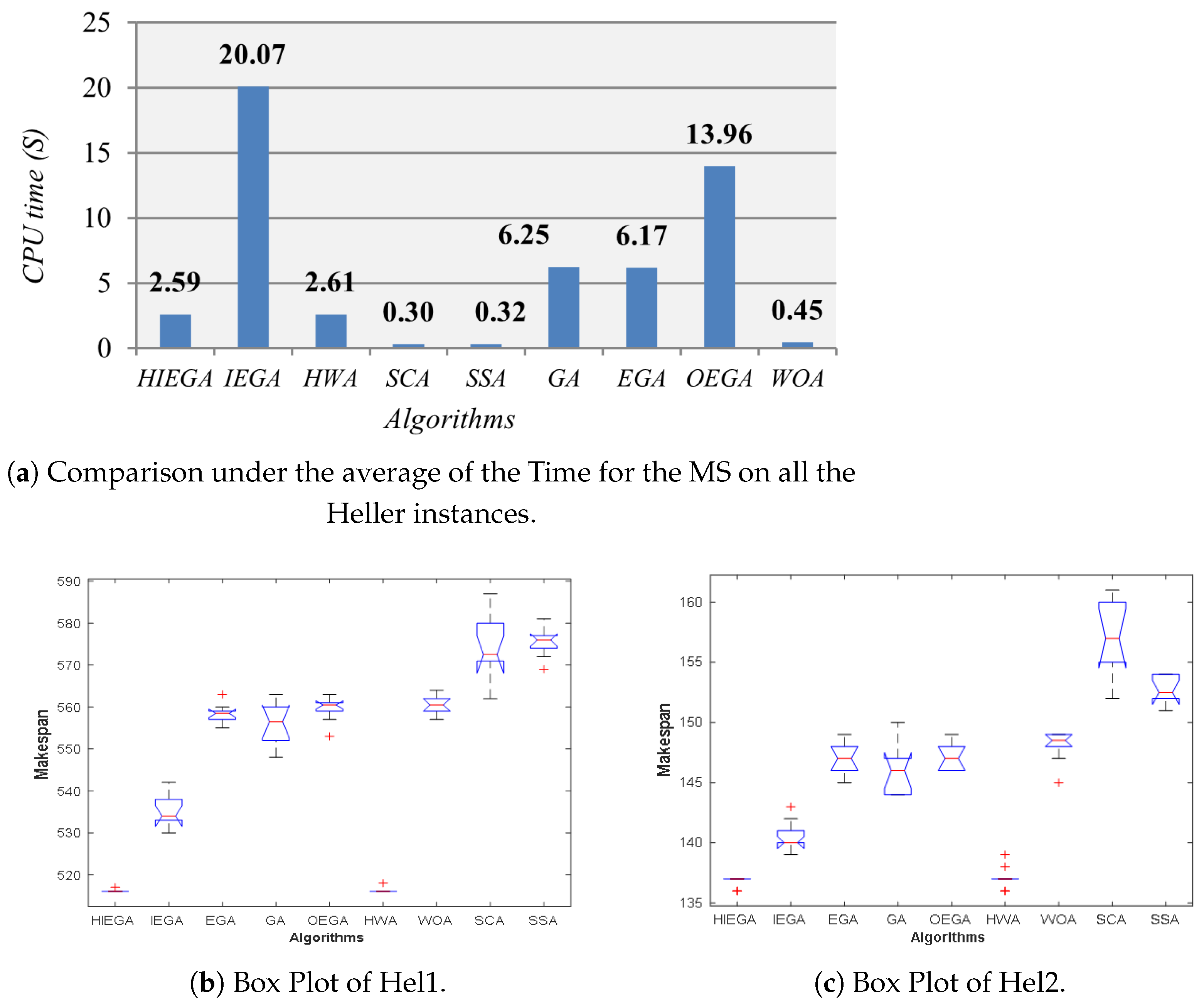
3.12. Comparison under CPU Time and BoxPLot
For knowing the speedup of each algorithm, we calculate the average of the CPU time needed by each algorithm until finishing implementing the instances of the Carlier and Heller, and this average value is introduced in Figure 7a. This figure told us that our proposed algorithm outperforms HWA, IEGA, GA, EGA, and OEGA and wins the first rank with a value of after SSA, SCA, and WOA. When comparing HIEGA with SSA, SCA, and WOA in terms of CPU time and MS, our proposed algorithm could significantly come true better outcomes at a reasonable time. In Figure 7b,c we compare the algorithms under the Boxplot for the values obtained by each one within 30 independent runs on Hel1 and Hel2, respectively. Inspecting this figure shows that IEGA could outperform all the algorithms except HIEGA and HWA. Also from this figure, we found that HIEGA could overcome HWA under the boxplot of Hel1 and Hel2. Generally, our proposed algorithms, IEGA and HIEGA, are competitive in comparison with the others.
4. Conclusions
This work presents the integration between the uniform crossover and the arithmetic crossover (UAC) to enhance the exploitation capability and alleviate stuck into local minima problems. After that, the UAC with re-initializing an individual selected randomly from the population through each iteration are combined in the EGA, to enhance its performance when tackling the PFSSP, which is a well-known scheduling problem applied in several industrial applications in a version, abbreviated as IEGA. Additionally, we integrate a LSS with the IEGA for strength its performance toward solving PFSSP; this version is abbreviated as HIEGA. HIEGA and IEGA are experimentally validated on three well-known benchmarks: Reeves, Heller, and Carlier, and compared with a number of the robust evolutionary and meta-heuristic algorithms. On the car instances, the proposed algorithm could reach a value of 0.001 for ARE; while for the Heller instances, it reaches a value of 0.003 for the same metric mentioned before; ultimately for the Reeve instances, a value of 0.020 for ARE is obtained by the proposed. The experimental outcomes show that IEGA and HIEGA is competitive with those algorithms.
Unfortunately, the computational cost of the proposed algorithm is slightly higher than some of the others used in comparison as our main limitation. Therefore, in our future work, we will work on overcoming the time complexity of those proposed by integrating them with some of the strategies like levy flight, and opposition theory until accelerating the convergence toward the best solution in less number of iterations. Additionally, we will incorporate extending our proposed algorithms to solve the open shop.
Author Contributions
Conceptualization, M.A.-B., R.M. and M.A.; methodology, M.A.-B., R.M., M.A.; software, M.A.-B., R.M.; validation, M.A., R.K.C. and M.J.R.; formal analysis, M.A.-B., R.M. and M.A.; investigation, R.K.C. and M.J.R.; resources, M.A.-B. and R.M.; data curation, M.A.-B., R.M. and M.A.; writing—original draft preparation, M.A.-B., R.M. and M.A.; writing—review and editing, R.K.C. and M.J.R.; visualization, M.A.-B. and R.M.; supervision, M.A. and M.J.R.; project administration, M.A.-B., R.M. and M.A.; funding acquisition, R.K.C. and M.J.R. All authors have read and agreed to the published version of the manuscript.
Funding
This research received no external funding.
Institutional Review Board Statement
The study did not involve humans or animals.
Informed Consent Statement
The study did not involve humans.
Data Availability Statement
We refer to data in the paper as following “The data sets used, canbe found in Available online: http://people.brunel.ac.uk/~mastjjb/jeb/orlib/files/flowshop1.txt” Brunel University London Subject: flowshop1.txt This file contains a set of 31 FSP test instances. These instances were contributed to OR-Library by Dirk C. Mattfeld (email [email protected]) and Rob J.M. Vaessens (email [email protected]). people.brunel.ac.uk.
Conflicts of Interest
The authors declare no conflict of interest.
References
- Johnson, S.M. Optimal two-and three-stage production schedules with setup times included. Naval Res. Logist. Q. 1954, 1, 61–68. [Google Scholar] [CrossRef]
- Gao, J.; Chen, R. An NEH-based heuristic algorithm for distributed permutation flowshop scheduling problems. Sci. Res. Essays 2011, 6, 3094–3100. [Google Scholar]
- Sauvey, C.; Sauer, N. Two NEH Heuristic Improvements for Flowshop Scheduling Problem with Makespan Criterion. Algorithms 2020, 13, 112. [Google Scholar] [CrossRef]
- Wang, H.; Wang, W.; Sun, H.; Cui, Z.; Rahnamayan, S.; Zeng, S. A new cuckoo search algorithm with hybrid strategies for flow shop scheduling problems. Soft Comput. 2017, 21, 4297–4307. [Google Scholar] [CrossRef]
- Kalczynski, P.J.; Kamburowski, J. An improved NEH heuristic to minimize makespan in permutation flow shops. Comput. Operat. Res. 2008, 35, 3001–3008. [Google Scholar]
- Dong, X.; Huang, H.; Chen, P. An improved NEH-based heuristic for the permutation flowshop problem. Comput. Operat. Res. 2008, 35, 3962–3968. [Google Scholar] [CrossRef]
- Zhang, S.J.; Gu, X.S.; Zhou, F.N. An improved discrete migrating birds optimization algorithm for the no-wait flow shop scheduling problem. IEEE Access 2020, 8, 99380–99392. [Google Scholar]
- Govindan, K.; Balasundaram, R.; Baskar, N.; Asokan, P. A hybrid approach for minimizing makespan in permutation flowshop scheduling. J. Syst. Sci. Syst. Eng. 2017, 26, 50–76. [Google Scholar] [CrossRef]
- Liu, Y.; Yin, M.; Gu, W. An effective differential evolution algorithm for permutation flow shop scheduling problem. Appl. Math. Comput. 2014, 248, 143–159. [Google Scholar] [CrossRef]
- Ding, J.Y.; Song, S.; Zhang, R.; Zhou, S.; Wu, C. A novel block-shifting simulated annealing algorithm for the no-wait flowshop scheduling problem. In Proceedings of the 2015 IEEE Congress on Evolutionary Computation (CEC), IEEE, Sendai, Japan, 25–28 May 2015; pp. 2768–2774. [Google Scholar]
- Sanjeev Kumar, R.; Padmanaban, K.; Rajkumar, M. Minimizing makespan and total flow time in permutation flow shop scheduling problems using modified gravitational emulation local search algorithm. Proc. Instit. Mech. Eng. Part B J. Eng. Manufac. 2018, 232, 534–545. [Google Scholar] [CrossRef]
- Reeves, C.R. A genetic algorithm for flowshop sequencing. Comput. Operat. Res. 1995, 22, 5–13. [Google Scholar] [CrossRef]
- Liu, B.; Wang, L.; Jin, Y.H. An effective PSO-based memetic algorithm for flow shop scheduling. IEEE Trans. Syst. Man Cybern. Part B 2007, 37, 18–27. [Google Scholar] [CrossRef] [PubMed]
- Xie, Z.; Zhang, C.; Shao, X.; Lin, W.; Zhu, H. An effective hybrid teaching–learning-based optimization algorithm for permutation flow shop scheduling problem. Adv. Eng. Softw. 2014, 77, 35–47. [Google Scholar] [CrossRef]
- Zhao, F.; Liu, H.; Zhang, Y.; Ma, W.; Zhang, C. A discrete water wave optimization algorithm for no-wait flow shop scheduling problem. Expert Syst. Appl. 2018, 91, 347–363. [Google Scholar] [CrossRef]
- Shareh, M.B.; Bargh, S.H.; Hosseinabadi, A.A.R.; Slowik, A. An improved bat optimization algorithm to solve the tasks scheduling problem in open shop. Neur. Comput. Appl. 2020, 1–15. [Google Scholar] [CrossRef]
- Li, B.B.; Wang, L.; Liu, B. An effective PSO-based hybrid algorithm for multiobjective permutation flow shop scheduling. IEEE Trans. Syst. Man Cybern. Part A Syst. Hum. 2008, 38, 818–831. [Google Scholar] [CrossRef]
- Priya, A.; Sahana, S.K. Multiprocessor scheduling based on evolutionary technique for solving permutation flow shop problem. IEEE Access 2020, 8, 53151–53161. [Google Scholar] [CrossRef]
- Pang, X.; Xue, H.; Tseng, M.L.; Lim, M.K.; Liu, K. Hybrid Flow Shop Scheduling Problems Using Improved Fireworks Algorithm for Permutation. Appl. Sci. 2020, 10, 1174. [Google Scholar]
- Mishra, A.; Shrivastava, D. A discrete Jaya algorithm for permutation flow-shop scheduling problem. Int. J. Ind. Eng. Comput. 2020, 11, 415–428. [Google Scholar] [CrossRef]
- Mirjalili, S.; Gandomi, A.H.; Mirjalili, S.Z.; Saremi, S.; Faris, H.; Mirjalili, S.M. Salp Swarm Algorithm: A bio-inspired optimizer for engineering design problems. Adv. Eng. Softw. 2017, 114, 163–191. [Google Scholar] [CrossRef]
- Mirjalili, S.; Lewis, A. The whale optimization algorithm. Adv. Eng. Softw. 2016, 95, 51–67. [Google Scholar] [CrossRef]
- Mirjalili, S. SCA: A sine cosine algorithm for solving optimization problems. Knowledge-Based Syst. 2016, 96, 120–133. [Google Scholar] [CrossRef]
- Abdel-Basset, M.; Mohamed, R.; Mirjalili, S. A novel Whale Optimization Algorithm integrated with Nelder–Mead simplex for multi-objective optimization problems. Knowl. Based Syst. 2020, 212, 106619. [Google Scholar] [CrossRef]
- Abualigah, L.; Shehab, M.; Alshinwan, M.; Alabool, H. Salp swarm algorithm: A comprehensive survey. Neural Comput. Appl. 2019, 1–21. [Google Scholar] [CrossRef]
- Abdel-Basset, M.; El-Shahat, D.; Deb, K.; Abouhawwash, M. Energy-aware whale optimization algorithm for real-time task scheduling in multiprocessor systems. Appl. Soft Comput. 2020, 93, 106349. [Google Scholar] [CrossRef]
- Zhang, X.; Guo, P.; Zhang, H.; Yao, J. Hybrid Particle Swarm Optimization Algorithm for Process Planning. Mathematics 2020, 8, 1745. [Google Scholar] [CrossRef]
- Ren, T.; Zhang, Y.; Cheng, S.R.; Wu, C.C.; Zhang, M.; Chang, B.Y.; Wang, X.Y.; Zhao, P. Effective Heuristic Algorithms Solving the Jobshop Scheduling Problem with Release Dates. Mathematics 2020, 8, 1221. [Google Scholar] [CrossRef]
- Cosma, O.; Pop, P.C.; Sabo, C. An Efficient Hybrid Genetic Approach for Solving the Two-Stage Supply Chain Network Design Problem with Fixed Costs. Mathematics 2020, 8, 712. [Google Scholar] [CrossRef]
- Abdel-Basset, M.; Manogaran, G.; El-Shahat, D.; Mirjalili, S. A hybrid whale optimization algorithm based on local search strategy for the permutation flow shop scheduling problem. Future Gener. Comput. Syst. 2018, 85, 129–145. [Google Scholar] [CrossRef] [Green Version]
- Goldberg, D.E.; Holland, J.H. Genetic Algorithms. Mach. Learn. 1988, 3, 95–99. [Google Scholar] [CrossRef]
- Holland, J.H. Genetic algorithms. Sci. Am. 1992, 267, 66–73. [Google Scholar] [CrossRef]
- Abdel-Basset, M.; Mohamed, R.; Abouhawwash, M. Balanced multi-objective optimization algorithm using improvement based reference points approach. Swarm Evol. Comput. 2020, 60, 100791. [Google Scholar] [CrossRef]
- Li, X.; Yin, M. An opposition-based differential evolution algorithm for permutation flow shop scheduling based on diversity measure. Adv. Eng. Softw. 2013, 55, 10–31. [Google Scholar] [CrossRef]
- Blickle, T.; Thiele, L. A Mathematical Analysis of Tournament Selection; ICGA Citeseer; Morgan Kaufmann: San Francisco, CA, USA, 1995; Volume 95, pp. 9–15. [Google Scholar]
- Semenkin, E.; Semenkina, M. Self-configuring genetic algorithm with modified uniform crossover operator. In Proceedings of the International Conference in Swarm Intelligence, Brussels, Belgium, 12–14 September 2012; Springer: Berlin/Heidelberg, Germany, 2012; pp. 414–421. [Google Scholar]
- Xiang, W. Analysis of the time complexity of quick sort algorithm. In Proceedings of the 2011 International Conference on Information Management, Innovation Management and Industrial Engineering, IEEE, Shenzhen, China, 26–27 November 2011; Volume 1, pp. 408–410. [Google Scholar]
- Carlier, J. Ordonnancements a contraintes disjonctives. RAIRO-Operat. Res. 1978, 12, 333–350. [Google Scholar] [CrossRef] [Green Version]
- Heller, J. Some numerical experiments for an M× J flow shop and its decision-theoretical aspects. Operat. Res. 1960, 8, 178–184. [Google Scholar] [CrossRef]
- Ancău, M. On solving flowshop scheduling problems. Proc. Roman. Acad. Ser. A 2012, 13, 71–79. [Google Scholar]
Figure 1.
Illustration for a real-value solution.

Figure 2.
Different genetic operators.

Figure 3.
The sensitivity analysis for the genetic parameters introduced.

Figure 4.
Comparison among algorithms on the car instances.

Figure 5.
Comparison under the average of ARE on all the Reeve instances.

Figure 6.
Comparison among algorithms on the Heller instances.

Figure 7.
Comparison among algorithms under CPU time and Box-plot for the makespan on the Heller instances.
Figure 7.
Comparison among algorithms under CPU time and Box-plot for the makespan on the Heller instances.


Table 1.
The dataset descriptions.
| Carlier, Heller, Reeves Benchmarks | |||||||
|---|---|---|---|---|---|---|---|
| Name | n | m | Name | n | m | ||
| Car01 | 11 | 5 | 7038 | Rec05 | 20 | 5 | 1242 |
| Car02 | 13 | 4 | 7166 | Rec07 | 20 | 10 | 1566 |
| Car03 | 12 | 5 | 7312 | Rec09 | 20 | 10 | 1537 |
| Car04 | 14 | 4 | 8003 | Rec11 | 20 | 10 | 1431 |
| Car05 | 10 | 6 | 7720 | Rec13 | 20 | 15 | 1930 |
| Car06 | 8 | 9 | 8505 | Rec15 | 20 | 15 | 1950 |
| Car07 | 7 | 7 | 6590 | Rec17 | 20 | 15 | 1902 |
| Car08 | 8 | 8 | 8366 | Rec19 | 30 | 10 | 2017 |
| Hel1 | 20 | 10 | 516 | Rec21 | 30 | 10 | 2011 |
| Hel2 | 100 | 10 | 136 | Rec37 | 75 | 20 | 4951 |
| Rec01 | 20 | 5 | 1247 | Rec39 | 75 | 20 | 5087 |
| Rec03 | 20 | 5 | 1109 | Rec41 | 75 | 20 | 4960 |
Table 2.
The parameters of the algorithms.
| GA, EGA, IEGA, OEGA and IEGA | HWA, HIEGA | ||
|---|---|---|---|
| CR | 0.8 | LSP | 0.01 |
| MR | 0.02 | BS P | 5 0.8 |
Table 3.
Outcomes of different performance metrics on the Car instances (Car01–Car06).
| Instances | Algorithm | BRE | WRE | ARE | SD | ||
|---|---|---|---|---|---|---|---|
| Car01 | HIEGA | 7038 | 0 | 0 | 0 | 7038 | 0 |
| IEGA | 0 | 0 | 0 | 7038 | 0 | ||
| HWA | 0 | 0 | 0 | 7038 | 0 | ||
| SCA | 0 | 0.171213 | 0.088562 | 7661.3 | 305.406849 | ||
| SSA | 0 | 0.122336 | 0.064303 | 7490.566667 | 226.370593 | ||
| GA | 0 | 0 | 0 | 7038 | 0 | ||
| EGA | 0 | 0.002699 | 0.000090 | 7038.633333 | 3.410604 | ||
| OEGA | 0 | 0 | 0 | 7038 | 0 | ||
| WOA | 0 | 0.042484 | 0.004244 | 7067.866667 | 66.693195 | ||
| Car02 | HIEGA | 7166 | 0 | 0 | 0 | 7166 | 0 |
| IEGA | 0 | 0.029305 | 0.018504 | 7298.6 | 94.769756 | ||
| HWA | 0 | 0 | 0 | 7166 | 0 | ||
| SCA | 0.084706 | 0.171365 | 0.130398 | 8100.433333 | 158.832130 | ||
| SSA | 0.056377 | 0.143734 | 0.099660 | 7880.166667 | 139.553116 | ||
| GA | 0.007257 | 0.055679 | 0.031352 | 7390.666667 | 62.308016 | ||
| EGA | 0 | 0.094334 | 0.037957 | 7438 | 118.735279 | ||
| OEGA | 0 | 0.059029 | 0.033078 | 7403.033333 | 94.837223 | ||
| WOA | 0 | 0.063634 | 0.037687 | 7436.066667 | 119.013146 | ||
| Car03 | HIEGA | 7312 | 0 | 0.011898 | 0.003597 | 7338.3 | 28.709058 |
| IEGA | 0.007385 | 0.049644 | 0.027922 | 7516.166667 | 85.491942 | ||
| HWA | 0 | 0.011898 | 0.006524 | 7359.7 | 34.085334 | ||
| SCA | 0.056483 | 0.184628 | 0.127010 | 8240.7 | 268.999771 | ||
| SSA | 0.035968 | 0.111324 | 0.076067 | 7868.2 | 170.196044 | ||
| GA | 0.011898 | 0.054431 | 0.028679 | 7521.7 | 87.041044 | ||
| EGA | 0.011898 | 0.044037 | 0.026044 | 7502.433333 | 72.344861 | ||
| OEGA | 0.006018 | 0.054431 | 0.032891 | 7552.5 | 65.858308 | ||
| WOA | 0.011898 | 0.056483 | 0.035161 | 7569.1 | 73.710402 | ||
| Car04 | HIEGA | 8003 | 0 | 0 | 0 | 8003 | 0 |
| IEGA | 0 | 0.011746 | 0.001141 | 8012.133333 | 22.399008 | ||
| HWA | 0 | 0 | 0 | 8003 | 0 | ||
| SCA | 0.052480 | 0.148819 | 0.091095 | 8732.033333 | 218.220146 | ||
| SSA | 0.018618 | 0.134699 | 0.070865 | 8570.133333 | 200.441468 | ||
| GA | 0 | 0.025366 | 0.004823 | 8041.6 | 56.202372 | ||
| EGA | 0 | 0.016244 | 0.006702 | 8056.633333 | 58.819772 | ||
| OEGA | 0 | 0.028239 | 0.012475 | 8102.833333 | 67.356803 | ||
| WOA | 0.000625 | 0.052480 | 0.015965 | 8130.766667 | 77.604847 | ||
| Car05 | HIEGA | 7720 | 0 | 0.013083 | 0.002988 | 7743.066667 | 33.402528 |
| IEGA | 0 | 0.034845 | 0.010734 | 7802.866667 | 49.143147 | ||
| HWA | 0 | 0.013083 | 0.003105 | 7743.966667 | 31.594813 | ||
| SCA | 0.038472 | 0.118005 | 0.078001 | 8322.166667 | 164.803536 | ||
| SSA | 0.002332 | 0.118912 | 0.024188 | 7906.733333 | 207.587079 | ||
| GA | 0 | 0.019819 | 0.010289 | 7799.433333 | 40.596948 | ||
| EGA | 0.003886 | 0.017358 | 0.010406 | 7800.333333 | 29.777322 | ||
| OEGA | 0 | 0.013989 | 0.006503 | 7770.2 | 29.221453 | ||
| WOA | 0.001554 | 0.018782 | 0.010622 | 7802 | 43.109937 | ||
| Car06 | HIEGA | 8505 | 0 | 0.007643 | 0.002802 | 8528.833333 | 31.3231366 |
| IEGA | 0 | 0.061023 | 0.021105 | 8684.5 | 147.216337 | ||
| HWA | 0 | 0.007643 | 0.003821 | 8537.5 | 32.5 | ||
| SCA | 0.054321 | 0.144386 | 0.088309 | 9256.066667 | 184.081311 | ||
| SSA | 0.007643 | 0.123691 | 0.044158 | 8880.566667 | 251.156483 | ||
| GA | 0 | 0.058554 | 0.016477 | 8645.133333 | 127.213923 | ||
| EGA | 0 | 0.051382 | 0.019075 | 8667.233333 | 131.723115 | ||
| OEGA | 0 | 0.041152 | 0.016899 | 8648.733333 | 105.884507 | ||
| WOA | 0 | 0.029277 | 0.011515 | 8602.933333 | 96.881004 |
Bold values indicate the best outcomes.
Table 4.
Outcomes of different performance metrics on the Car instances (Car07–Car08).
| Instances | Algorithm | BRE | WRE | ARE | SD | ||
|---|---|---|---|---|---|---|---|
| Car07 | HIEGA | 6590 | 0 | 0.008043 | 0 | 6591.766667 | 0 |
| IEGA | 0 | 0.008043 | 0.001877 | 6602.366667 | 22.416487 | ||
| HWA | 0 | 0.008043 | 0.001340 | 6598.833333 | 19.751934 | ||
| SCA | 0.014416 | 0.130197 | 0.071259 | 7059.6 | 195.841024 | ||
| SSA | 0 | 0.145827 | 0.035225 | 6822.133333 | 230.693842 | ||
| GA | 0 | 0.025797 | 0.002155 | 6604.2 | 36.750873 | ||
| EGA | 0 | 0.025797 | 0.002403 | 6605.833333 | 37.018989 | ||
| OEGA | 0 | 0.008346 | 0.002155 | 6604.2 | 23.550513 | ||
| WOA | 0 | 0.008346 | 0.001897 | 6602.5 | 22.662377 | ||
| Car08 | HIEGA | 8366 | 0 | 0.008346 | 0.001897 | 6602.5 | 22.662377 |
| IEGA | 0 | 0 | 0 | 8366 | 0 | ||
| HWA | 0 | 0.035620 | 0.008179 | 8434.433333 | 64.081554 | ||
| SCA | 0 | 0 | 0 | 8366 | 0 | ||
| SSA | 0.010877 | 0.093593 | 0.059527 | 8864 | 169.176239 | ||
| GA | 0.005139 | 0.071002 | 0.025922 | 8582.866667 | 127.503656 | ||
| EGA | 0 | 0.031198 | 0.011017 | 8458.166667 | 65.852909 | ||
| OEGA | 0 | 0.030002 | 0.010774 | 8456.133333 | 53.485658 | ||
| WOA | 0 | 0.012789 | 0.005610 | 8412.933333 | 35.052278 |
Bold values indicate the best outcomes.
Table 5.
Outcomes of different performance metrics on the Reeve instances (Rec01–Rec11).
| Instances | Algorithm | BRE | WRE | ARE | SD | ||
|---|---|---|---|---|---|---|---|
| Rec01 | HIEGA | 1247 | 0 | 0.019246 | 0.002834 | 1250.533333 | 4.828618 |
| IEGA | 0.052125 | 0.106656 | 0.070783 | 1335.266667 | 14.534862 | ||
| HWA | 0.001604 | 0.051323 | 0.006977 | 1255.7 | 14.744829 | ||
| SCA | 0.109864 | 0.198075 | 0.157017 | 1442.8 | 20.972045 | ||
| SSA | 0.086608 | 0.178027 | 0.137423 | 1418.366667 | 25.921013 | ||
| GA | 0.063352 | 0.100241 | 0.082625 | 1350.033333 | 13.816616 | ||
| EGA | 0.063352 | 0.109864 | 0.082304 | 1349.633333 | 13.352861 | ||
| OEGA | 0.058541 | 0.103448 | 0.081476 | 1348.6 | 15.098786 | ||
| WOA | 0.074579 | 0.120289 | 0.092515 | 1362.366667 | 14.155054 | ||
| Rec03 | HIEGA | 1109 | 0 | 0.021641 | 0.002164 | 1111.4 | 4.644710 |
| IEGA | 0.007214 | 0.061317 | 0.040517 | 1153.933333 | 13.921047 | ||
| HWA | 0 | 0.021641 | 0.002946 | 1112.266667 | 6.065934 | ||
| SCA | 0.102795 | 0.210099 | 0.152901 | 1278.566667 | 32.871146 | ||
| SSA | 0.078449 | 0.167719 | 0.119748 | 1241.8 | 31.186963 | ||
| GA | 0.030658 | 0.067629 | 0.052329 | 1167.033333 | 11.223438 | ||
| EGA | 0.029757 | 0.089269 | 0.056748 | 1171.933333 | 14.449759 | ||
| OEGA | 0.032462 | 0.069432 | 0.052059 | 1166.733333 | 9.688252 | ||
| WOA | 0.038774 | 0.099189 | 0.073129 | 1190.1 | 14.839924 | ||
| Rec05 | HIEGA | 1242 | 0.002416 | 0.018519 | 0.006871 | 1250.533333 | 5.481687 |
| IEGA | 0.012077 | 0.056361 | 0.034568 | 1284.933333 | 11.744313 | ||
| HWA | 0.002416 | 0.011272 | 0.004938 | 1248.133333 | 4.177187 | ||
| SCA | 0.042673 | 0.153784 | 0.115996 | 1386.066667 | 26.293134 | ||
| SSA | 0.045894 | 0.134461 | 0.097236 | 1362.766667 | 26.297888 | ||
| GA | 0.024959 | 0.060387 | 0.043156 | 1295.6 | 9.704295 | ||
| EGA | 0.017713 | 0.070048 | 0.043774 | 1296.366667 | 14.969933 | ||
| OEGA | 0.026570 | 0.058776 | 0.042002 | 1294.166667 | 9.757333 | ||
| WOA | 0.029791 | 0.060387 | 0.048282 | 1301.966667 | 9.809802 | ||
| Rec07 | HIEGA | 1566 | 0 | 0.011494 | 0.007663 | 1578 | 8.485281 |
| IEGA | 0.035759 | 0.087484 | 0.056939 | 1655.166667 | 20.448445 | ||
| HWA | 0 | 0.011494 | 0.007791 | 1578.2 | 8.268011 | ||
| SCA | 0.093231 | 0.188378 | 0.147829 | 1797.5 | 33.795217 | ||
| SSA | 0.082376 | 0.173052 | 0.120945 | 1755.4 | 39.244193 | ||
| GA | 0.042146 | 0.100894 | 0.069199 | 1674.366667 | 18.948146 | ||
| EGA | 0.045338 | 0.101533 | 0.073159 | 1680.566667 | 22.496938 | ||
| OEGA | 0.044699 | 0.084929 | 0.067497 | 1671.7 | 14.512409 | ||
| WOA | 0.051086 | 0.096424 | 0.077203 | 1686.9 | 15.712734 | ||
| Rec09 | HIEGA | 1537 | 0 | 0.063761 | 0.014769 | 1559.7 | 21.506820 |
| IEGA | 0.051399 | 0.116461 | 0.089091 | 1673.933333 | 22.152401 | ||
| HWA | 0 | 0.042290 | 0.017393 | 1563.733333 | 16.958643 | ||
| SCA | 0.130124 | 0.202342 | 0.164867 | 1790.4 | 28.841637 | ||
| SSA | 0.068315 | 0.162004 | 0.118174 | 1718.633333 | 35.250989 | ||
| GA | 0.074171 | 0.117111 | 0.094860 | 1682.8 | 19.482299 | ||
| EGA | 0.062459 | 0.121015 | 0.097636 | 1687.066667 | 20.602481 | ||
| OEGA | 0.065712 | 0.113208 | 0.095316 | 1683.5 | 17.659275 | ||
| WOA | 0.060508 | 0.124268 | 0.099349 | 1689.7 | 22.564205 | ||
| Rec11 | HIEGA | 1431 | 0 | 0.0433263 | 0.014256 | 1451.4 | 17.779388 |
| IEGA | 0.093640 | 0.141858 | 0.117027 | 1598.466667 | 18.990758 | ||
| HWA | 0 | 0.040531 | 0.017353 | 1455.833333 | 17.384060 | ||
| SCA | 0.149545 | 0.220824 | 0.194805 | 1709.766667 | 27.304069 | ||
| SSA | 0.095737 | 0.198462 | 0.156836 | 1655.433333 | 30.650376 | ||
| GA | 0.096436 | 0.145352 | 0.122362 | 1606.1 | 16.213882 | ||
| EGA | 0.082459 | 0.150943 | 0.123526 | 1607.766667 | 19.653130 | ||
| OEGA | 0.100628 | 0.139063 | 0.119613 | 1602.166667 | 14.973495 | ||
| WOA | 0.088050 | 0.136268 | 0.118518 | 1600.6 | 15.632444 |
Bold values indicate the best outcomes.
Table 6.
Outcomes of different performance metrics on the Reeve instances (Rec13–Rec25).
| Instances | Algorithm | BRE | WRE | ARE | SD | ||
|---|---|---|---|---|---|---|---|
| Rec13 | HIEGA | 1930 | 0 | 0.038342 | 0.015664 | 1960.233333 | 15.683714 |
| IEGA | 0.046632 | 0.118134 | 0.076131 | 2076.933333 | 29.532957 | ||
| HWA | 0.002072 | 0.044559 | 0.019153 | 1966.966667 | 16.592133 | ||
| SCA | 0.122797 | 0.214507 | 0.164162 | 2246.833333 | 35.753865 | ||
| SSA | 0.109844 | 0.182383 | 0.135716 | 2191.933333 | 32.857199 | ||
| GA | 0.078238 | 0.121761 | 0.096269 | 2115.8 | 22.456476 | ||
| EGA | 0.069948 | 0.130569 | 0.094801 | 2112.966667 | 29.238654 | ||
| OEGA | 0.088082 | 0.119171 | 0.100690 | 2124.333333 | 17.376868 | ||
| WOA | 0.096373 | 0.127979 | 0.109706 | 2141.733333 | 14.042633 | ||
| Rec15 | HIEGA | 1950 | 0.004615 | 0.098974 | 0.024290 | 1997.366667 | 35.095567 |
| IEGA | 0.047692 | 0.098974 | 0.068974 | 2084.5 | 19.416058 | ||
| HWA | 0.005128 | 0.042564 | 0.018461 | 1986 | 21.594752 | ||
| SCA | 0.090769 | 0.168205 | 0.141538 | 2226 | 34.466408 | ||
| SSA | 0.070256 | 0.131794 | 0.108085 | 2160.766667 | 30.206713 | ||
| GA | 0.063589 | 0.106666 | 0.084700 | 2115.166667 | 22.764128 | ||
| EGA | 0.061538 | 0.101025 | 0.083641 | 2113.1 | 18.758731 | ||
| OEGA | 0.06 | 0.097948 | 0.080700 | 2107.366667 | 19.027144 | ||
| WOA | 0.055384 | 0.092307 | 0.081982 | 2109.866667 | 14.548157 | ||
| Rec17 | HIEGA | 1902 | 0.017350 | 0.082544 | 0.035173 | 1968.9 | 25.981211 |
| IEGA | 0.067297 | 0.114090 | 0.093305 | 2079.466667 | 24.349857 | ||
| HWA | 0 | 0.058359 | 0.027024 | 1953.4 | 20.878378 | ||
| SCA | 0.127760 | 0.206624 | 0.170347 | 2226 | 32.794308 | ||
| SSA | 0.107781 | 0.179285 | 0.135278 | 2159.3 | 32.444979 | ||
| GA | 0.074658 | 0.121976 | 0.106151 | 2103.9 | 20.932192 | ||
| EGA | 0.088853 | 0.137224 | 0.108307 | 2108 | 19.832633 | ||
| OEGA | 0.090431 | 0.128811 | 0.114335 | 2119.466667 | 16.995555 | ||
| WOA | 0.097791 | 0.136172 | 0.114879 | 2120.5 | 18.067927 | ||
| Rec19 | HIEGA | 2017 | 0.044124 | 0.187902 | 0.058139 | 2134.266667 | 49.683621 |
| IEGA | 0.123946 | 0.163113 | 0.144752 | 2308.966667 | 21.393898 | ||
| HWA | 0.042141 | 0.069410 | 0.055197 | 2128.333333 | 11.950825 | ||
| SCA | 0.176995 | 0.258800 | 0.230325 | 2481.566667 | 36.693944 | ||
| SSA | 0.153197 | 0.238968 | 0.205982 | 2432.466667 | 35.916322 | ||
| GA | 0.143777 | 0.179970 | 0.163427 | 2346.633333 | 19.460187 | ||
| EGA | 0.136836 | 0.184928 | 0.163609 | 2347 | 21.776133 | ||
| OEGA | 0.143777 | 0.174020 | 0.160337 | 2340.4 | 18.045498 | ||
| WOA | 0.134358 | 0.195835 | 0.175260 | 2370.5 | 26.722961 | ||
| Rec21 | HIEGA | 2011 | 0.013426 | 0.019393 | 0.018680 | 2048.566667 | 2.603629 |
| IEGA | 0.074589 | 0.138736 | 0.108238 | 2228.666667 | 28.311756 | ||
| HWA | 0.009945 | 0.019393 | 0.018680 | 2048.566667 | 3.630273 | ||
| SCA | 0.165092 | 0.228741 | 0.196784 | 2406.733333 | 33.423478 | ||
| SSA | 0.128294 | 0.203381 | 0.168788 | 2350.433333 | 34.844113 | ||
| GA | 0.087021 | 0.150174 | 0.126255 | 2264.9 | 24.064288 | ||
| EGA | 0.104922 | 0.148185 | 0.127697 | 2267.8 | 21.487050 | ||
| OEGA | 0.108403 | 0.152163 | 0.129355 | 2271.133333 | 20.170495 | ||
| WOA | 0.109895 | 0.148185 | 0.133731 | 2279.933333 | 19.177996 | ||
| Rec23 | HIEGA | 2011 | 0.004972 | 0.034808 | 0.017918 | 2047.033333 | 14.855937 |
| IEGA | 0.085529 | 0.141223 | 0.110923 | 2234.066667 | 27.282391 | ||
| HWA | 0.004972 | 0.036300 | 0.016194 | 2043.566667 | 14.247066 | ||
| SCA | 0.137245 | 0.220288 | 0.186507 | 2386.066667 | 39.107487 | ||
| SSA | 0.139234 | 0.206365 | 0.165108 | 2343.033333 | 32.162590 | ||
| GA | 0.110890 | 0.158130 | 0.129587 | 2271.6 | 19.491194 | ||
| EGA | 0.104425 | 0.151665 | 0.128244 | 2268.9 | 20.799599 | ||
| OEGA | 0.116360 | 0.146195 | 0.131990 | 2276.433333 | 15.329021 | ||
| WOA | 0.112879 | 0.151168 | 0.131659 | 2275.766667 | 18.322451 | ||
| Rec25 | HIEGA | 2513 | 0.007958 | 0.044966 | 0.026754 | 2580.233333 | 19.095694 |
| IEGA | 0.082371 | 0.121368 | 0.106685 | 2781.1 | 22.530497 | ||
| HWA | 0.014325 | 0.045364 | 0.027616 | 2582.4 | 16.987446 | ||
| SCA | 0.155590 | 0.204934 | 0.176588 | 2956.766667 | 36.271828 | ||
| SSA | 0.108635 | 0.188221 | 0.150245 | 2890.566667 | 41.364786 | ||
| GA | 0.102268 | 0.139673 | 0.122735 | 2821.433333 | 20.817754 | ||
| EGA | 0.092319 | 0.147632 | 0.127749 | 2834.033333 | 25.235534 | ||
| OEGA | 0.097493 | 0.136490 | 0.122708 | 2821.366667 | 19.693456 | ||
| WOA | 0.107043 | 0.149224 | 0.127152 | 2832.533333 | 24.555696 |
Bold values indicate the best outcomes.
Table 7.
Outcomes of different performance metrics on the Reeve instances (Rec27–Rec37).
| Instances | Algorithm | BRE | WRE | ARE | SD | ||
|---|---|---|---|---|---|---|---|
| Rec27 | HIEGA | 2373 | 0.008006 | 0.036662 | 0.019272 | 2418.733333 | 16.641180 |
| IEGA | 0.096923 | 0.147071 | 0.119047 | 2655.5 | 30.93945 | ||
| HWA | 0.010535 | 0.032027 | 0.019525 | 2419.333333 | 13.842767 | ||
| SCA | 0.170670 | 0.235988 | 0.202612 | 2853.8 | 46.058947 | ||
| SSA | 0.139907 | 0.209860 | 0.179898 | 2799.9 | 40.539980 | ||
| GA | 0.102823 | 0.160977 | 0.136311 | 2696.466667 | 36.165115 | ||
| EGA | 0.115887 | 0.153813 | 0.137772 | 2699.933333 | 20.720253 | ||
| OEGA | 0.088074 | 0.160556 | 0.139120 | 2703.133333 | 34.369301 | ||
| WOA | 0.112937 | 0.156342 | 0.137435 | 2699.133333 | 26.572834 | ||
| Rec29 | HIEGA | 2287 | 0.006121 | 0.042850 | 0.023597 | 2340.966667 | 22.394170 |
| IEGA | 0.101442 | 0.174901 | 0.142661 | 2613.266667 | 37.883974 | ||
| HWA | 0.007870 | 0.050284 | 0.027969 | 2350.966667 | 24.183304 | ||
| SCA | 0.195452 | 0.254044 | 0.225200 | 2802.033333 | 37.867737 | ||
| SSA | 0.157848 | 0.239178 | 0.192042 | 2726.2 | 43.699275 | ||
| GA | 0.140358 | 0.188019 | 0.162789 | 2659.3 | 27.098770 | ||
| EGA | 0.137297 | 0.191954 | 0.162075 | 2657.666667 | 25.819028 | ||
| OEGA | 0.132488 | 0.177962 | 0.159860 | 2652.6 | 25.210579 | ||
| WOA | 0.144731 | 0.186270 | 0.165573 | 2665.666667 | 25.373652 | ||
| Rec31 | HIEGA | 3045 | 0.002627 | 0.027586 | 0.016934 | 3096.566667 | 22.008609 |
| IEGA | 0.104433 | 0.146798 | 0.125473 | 3427.066667 | 39.693772 | ||
| HWA | 0.008867 | 0.037766 | 0.022375 | 3113.133333 | 20.418510 | ||
| SCA | 0.154351 | 0.210837 | 0.186097 | 3611.666667 | 34.852387 | ||
| SSA | 0.134318 | 0.198358 | 0.177329 | 3584.966667 | 42.869167 | ||
| GA | 0.127422 | 0.157635 | 0.140634 | 3473.233333 | 23.531090 | ||
| EGA | 0.122824 | 0.162233 | 0.142200 | 3478 | 23.359509 | ||
| OEGA | 0.122495 | 0.159277 | 0.143940 | 3483.3 | 27.282656 | ||
| WOA | 0.131362 | 0.159277 | 0.147071 | 3492.833333 | 25.139720 | ||
| Rec33 | HIEGA | 3114 | 0.001284 | 0.020231 | 0.008188 | 3139.5 | 10.883473 |
| IEGA | 0.074181 | 0.115606 | 0.098126 | 3419.566667 | 29.809040 | ||
| HWA | 0.001284 | 0.010276 | 0.008295 | 3139.833333 | 4.305681 | ||
| SCA | 0.150610 | 0.198137 | 0.173560 | 3654.466667 | 36.446063 | ||
| SSA | 0.121066 | 0.193962 | 0.162952 | 3621.433333 | 49.127509 | ||
| GA | 0.102761 | 0.136159 | 0.115403 | 3473.366667 | 22.817366 | ||
| EGA | 0.094091 | 0.137443 | 0.113690 | 3468.033333 | 33.271091 | ||
| OEGA | 0.107899 | 0.128131 | 0.118946 | 3484.4 | 18.307739 | ||
| WOA | 0.106294 | 0.140976 | 0.123389 | 3498.233333 | 27.813286 | ||
| Rec35 | HIEGA | 3277 | 0 | 0 | 0 | 3277 | 0 |
| IEGA | 0.044552 | 0.083918 | 0.063452 | 3484.933333 | 29.017159 | ||
| HWA | 0 | 0.000915 | 0.000030 | 3277.1 | 0.538516 | ||
| SCA | 0.105584 | 0.158986 | 0.132478 | 3711.133333 | 42.568950 | ||
| SSA | 0.089105 | 0.145865 | 0.120587 | 3672.166667 | 44.570605 | ||
| GA | 0.064693 | 0.092767 | 0.080327 | 3540.233333 | 25.608180 | ||
| EGA | 0.057064 | 0.101617 | 0.083084 | 3549.266667 | 34.247076 | ||
| OEGA | 0.065913 | 0.091852 | 0.083653 | 3551.133333 | 19.057340 | ||
| WOA | 0.046689 | 0.098870 | 0.085433 | 3556.966667 | 33.488787 | ||
| Rec37 | HIEGA | 4951 | 0.032922 | 0.056756 | 0.042227 | 5160.066667 | 27.546243 |
| IEGA | 0.146435 | 0.182791 | 0.167528 | 5780.433333 | 40.535320 | ||
| HWA | 0.023833 | 0.058372 | 0.044206 | 5169.866667 | 38.933904 | ||
| SCA | 0.185215 | 0.235710 | 0.216064 | 6020.733333 | 62.100957 | ||
| SSA | 0.184407 | 0.213492 | 0.198215 | 5932.366667 | 35.673971 | ||
| GA | 0.157140 | 0.188850 | 0.175708 | 5820.933333 | 35.789135 | ||
| EGA | 0.166229 | 0.191072 | 0.176395 | 5824.333333 | 31.882422 | ||
| OEGA | 0.154918 | 0.188244 | 0.176806 | 5826.366667 | 39.860994 | ||
| WOA | 0.153706 | 0.186225 | 0.176408 | 5824.4 | 31.813623 |
Bold values indicate the best outcomes.
Table 8.
Outcomes of different performance metrics on the Reeve instances (Rec39–Rec41).
| Instances | Algorithm | BRE | WRE | ARE | SD | ||
|---|---|---|---|---|---|---|---|
| Rec39 | HIEGA | 5087 | 0.013564 | 0.034598 | 0.022980 | 5203.9 | 27.544327 |
| IEGA | 0.113033 | 0.168665 | 0.145888 | 5829.133333 | 71.492066 | ||
| HWA | 0.011401 | 0.039512 | 0.025273 | 5215.566667 | 31.597134 | ||
| SCA | 0.179083 | 0.222528 | 0.198853 | 6098.566667 | 53.726271 | ||
| SSA | 0.159622 | 0.206211 | 0.182412 | 6014.933333 | 57.731524 | ||
| GA | 0.145862 | 0.170434 | 0.15824 | 5891.966667 | 33.412057 | ||
| EGA | 0.141930 | 0.175152 | 0.159229 | 5897 | 47.012055 | ||
| OEGA | 0.140554 | 0.167682 | 0.155527 | 5878.166667 | 35.096137 | ||
| WOA | 0.148810 | 0.177118 | 0.164635 | 5924.5 | 28.965209 | ||
| Rec41 | HIEGA | 4960 | 0.025637 | 0.050806 | 0.039227 | 5154.566667 | 28.312168 |
| IEGA | 0.146572 | 0.194354 | 0.169731 | 5801.866667 | 44.835055 | ||
| HWA | 0.028830 | 0.059072 | 0.043131 | 5173.933333 | 33.260520 | ||
| SCA | 0.197782 | 0.246774 | 0.227210 | 6086.966667 | 54.319108 | ||
| SSA | 0.194354 | 0.237903 | 0.213608 | 6019.5 | 52.392588 | ||
| GA | 0.170161 | 0.208467 | 0.187332 | 5889.166667 | 45.649449 | ||
| EGA | 0.171371 | 0.205040 | 0.187022 | 5887.633333 | 36.043014 | ||
| OEGA | 0.169758 | 0.198790 | 0.186444 | 5884.766667 | 30.707961 | ||
| WOA | 0.178225 | 0.201612 | 0.190732 | 5906.033333 | 29.825585 |
Bold values indicate the best outcomes.
Table 9.
Outcomes of the performance metrics on the Heller instances.
| Instances | Algorithm | BRE | WRE | ARE | SD | ||
|---|---|---|---|---|---|---|---|
| Hel1 | HIEGA | 516 | −0.001938 | 0.001938 | 0.000129 | 516.066666 | 0.442216 |
| IEGA | 0.042635 | 0.081395 | 0.067441 | 550.8 | 4.460194 | ||
| HWA | −0.001938 | 0.007751 | 0.000710 | 516.366666 | 1.079609 | ||
| SCA | 0.089147 | 0.141472 | 0.116085 | 575.9 | 4.928488 | ||
| SSA | 0.094961 | 0.122093 | 0.109043 | 572.266666 | 3.687215 | ||
| GA | 0.065891 | 0.094961 | 0.079715 | 557.133333 | 3.621540 | ||
| EGA | 0.065891 | 0.091085 | 0.079328 | 556.933333 | 3.511251 | ||
| OEGA | 0.071705 | 0.089147 | 0.080943 | 557.766666 | 2.499111 | ||
| WOA | 0.063953 | 0.094961 | 0.086627 | 560.7 | 2.876919 | ||
| Hel3 | HIEGA | 136 | 0 | 0.029411 | 0.006372 | 136.866666 | 0.718022 |
| IEGA | 0.029411 | 0.080882 | 0.056372 | 143.666666 | 1.776388 | ||
| HWA | 0 | 0.036764 | 0.007107 | 136.966666 | 0.982626 | ||
| SCA | 0.117647 | 0.183823 | 0.155882 | 157.2 | 2.150968 | ||
| SSA | 0.073529 | 0.161764 | 0.121813 | 152.566666 | 2.679344 | ||
| GA | 0.058823 | 0.095588 | 0.074019 | 146.066666 | 1.364632 | ||
| EGA | 0.044117 | 0.110294 | 0.077941 | 146.6 | 2.154065 | ||
| OEGA | 0.066176 | 0.095588 | 0.083823 | 147.4 | 1.113552 |
Bold values indicate the best outcomes.
Publisher’s Note: MDPI stays neutral with regard to jurisdictional claims in published maps and institutional affiliations. |
© 2021 by the authors. Licensee MDPI, Basel, Switzerland. This article is an open access article distributed under the terms and conditions of the Creative Commons Attribution (CC BY) license (http://creativecommons.org/licenses/by/4.0/).
Share and Cite
MDPI and ACS Style
Abdel-Basset, M.; Mohamed, R.; Abouhawwash, M.; Chakrabortty, R.K.; Ryan, M.J. A Simple and Effective Approach for Tackling the Permutation Flow Shop Scheduling Problem. Mathematics 2021, 9, 270. https://doi.org/10.3390/math9030270
AMA Style
Abdel-Basset M, Mohamed R, Abouhawwash M, Chakrabortty RK, Ryan MJ. A Simple and Effective Approach for Tackling the Permutation Flow Shop Scheduling Problem. Mathematics. 2021; 9(3):270. https://doi.org/10.3390/math9030270
Chicago/Turabian StyleAbdel-Basset, Mohamed, Reda Mohamed, Mohamed Abouhawwash, Ripon K. Chakrabortty, and Michael J. Ryan. 2021. "A Simple and Effective Approach for Tackling the Permutation Flow Shop Scheduling Problem" Mathematics 9, no. 3: 270. https://doi.org/10.3390/math9030270
Note that from the first issue of 2016, this journal uses article numbers instead of page numbers. See further details here.