Transient Electromagnetic Monitoring of Permafrost: Mathematical Modeling Based on Sumudu Integral Transform and Artificial Neural Networks

Abstract

Due to the ongoing global warming on the Earth, permafrost degradation has been extensively taking place, which poses a substantial threat to civil and industrial facilities and infrastructure elements, as well as to the utilization of natural resources in the Arctic and high-latitude regions. In order to prevent the negative consequences of permafrost thawing under the foundations of constructions, various geophysical techniques for monitoring permafrost have been proposed and applied so far: temperature, electrical, seismic and many others. We propose a cross-borehole exploration system for a high localization of target objects in the cryolithozone. A novel mathematical apparatus for three-dimensional modeling of transient electromagnetic signals by the vector finite element method has been developed. The original combination of the latter, the Sumudu integral transform and artificial neural networks makes it possible to examine spatially heterogeneous objects of the cryolithozone with a high contrast of geoelectric parameters, significantly reducing computational costs. We consider numerical simulation results of the transient electromagnetic monitoring of industrial facilities located on permafrost. The formation of a talik has been shown to significantly manifest itself in the measured electromagnetic responses, which enables timely prevention of industrial disasters and environmental catastrophes.

1. Introduction

Unceasing global warming and thawing of permafrost on the Earth in response to climate change have been reported in polar regions and at high elevations since about 1980. Numerical studies show that these processes will continue and are likely to accelerate [1]. Since the Arctic is warming two to four times faster than the worldwide average, permafrost carbon emissions in a changing Arctic additionally and steadily contribute to global warming [2]. A fast response of permafrost to the warming climate has also been documented for northeast Siberia [3].

Degrading permafrost poses a major threat to the sustainable growth of Arctic communities and utilization of natural resources in the region [4]. The extent of infrastructure damage is substantial, ca. 70% of infrastructure elements being at risk [5]. Permafrost degradation-related infrastructure costs are expected to reach hundreds of billions of US dollars by the middle of the 21st century; Russia is assumed to bear the highest burden of country-specific expenses [6]. Moreover, there is a serious environmental threat owing to the risk of contamination and mobilization of toxic substances in Arctic permafrost regions [7].

In this connection, timely monitoring and decision-making seem to be critical for the sustainable development and economy of Arctic and high-altitude cold regions. Among the target monitoring objects are: highways [8,9]; railway lines [10,11]; airport runways [12,13]; engineering constructions at oil [14] and gas [15] fields; thawing zones around production wells during hydrocarbon extraction [16,17]; oil and gas pipelines [18,19]; fuel storage tanks [20,21]; bridge foundations [22,23]; pile foundations of buildings [24,25]; power transmission lines [26,27].

To date, a variety of approaches to monitoring permafrost have been proposed: from space [28]; by means of interferometric synthetic aperture radar (InSAR) [29]; with unmanned aerial vehicles [30]; surface deformation monitoring [31]; ground-based [32] and cross-borehole [33] seismic monitoring [34].

Currently, the most ubiquitous approach towards permafrost monitoring is borehole temperature time-lapse surveys [35,36,37]. Next in abundance are geoelectric prospecting techniques, including their cross-borehole modifications and 3D data inversion: electrical resistivity tomography [38,39,40,41] and ground penetrating radar [42,43,44]. There exist experimental works that simulate resistivity monitoring of the active permafrost layer in laboratory conditions [45].

A scientific direction is developing that draws on the use of alternating electromagnetic field data and their subsequent 2D [46] and 3D [47,48] inversion as applied to cross-borehole permafrost monitoring.

Integration of geophysical techniques is actively involved to address the monitoring problem: time-lapse electrical resistivity tomography combined with ground temperature [49,50] and with frequency-domain electro-magnetometry measurements [51]; electrical resistivity tomography paired with ground penetrating radar [52].

With regard to permafrost monitoring, rapidly growing is the ground-based transient electromagnetic (TEM) technique [53,54]. There is successful experience in combining TEM and frequency sounding data for investigating permafrost and gas hydrates on the Arctic shelf [55]. At the same time, TEM borehole [56] and cross-borehole [57] varieties appear to have significant unrevealed potential.

The presented research is devoted to the theoretical development of a cross-borehole TEM technique for the purposes of permafrost monitoring [58]. Promising numerical simulation results have been obtained so far for highways [59] and fuel storage tanks [60]. A prototype of the cross-borehole exploration equipment has been created [61], followed by a series of successful field measurements [62].

The development and evolvement of novel geophysical technologies is conventionally based on highly efficient means of mathematical modeling of synthetic signals [34]. As part of the study, we consider an algorithm for three-dimensional modeling of electromagnetic pulses using the vector finite element method. The original combination of the latter with the Sumudu integral transform makes it possible to study spatially inhomogeneous objects with a high contrast of geoelectric parameters [63]. Moreover, to significantly reduce the computational costs, artificial neural networks toolkit is applied [64], which is known to be a reliable means of increasing the efficiency of electrical exploration data interpretation [65,66,67].

Selected cross-borehole exploration systems provide a means of achieving a high localization of a thawing area. We give examples of numerically simulated TEM permafrost monitoring signals beneath industrial facilities.

2. Mathematical Modeling of TEM Signals

2.1. Sumudu Integral Transform

The Sumudu integral transform was proposed in [68] as an alternative to the Laplace transform. It is defined as follows:

$$S[f(t)]={\int }_0^{\infty }\frac{1}{u}\mathit{exp}(-\frac{t}{u})f(t)dt=f(u).$$

(1)

If the original function f has an argument t, then the Sumudu image of this function has the same notation, but its argument is replaced by u. It should be noted that the Sumudu image of a real-valued function is also a real-valued function. Thus, in subsequent calculations, unlike using the Laplace or Fourier transform, there is no need to resort to complex numbers. In addition, the calculation of electromagnetic signals through the Fourier transform at late times after turning on the source becomes very expensive due to the need to integrate rapidly oscillating and weakly decaying integrands [69]. So, when finding the Sumudu image of a function, computational costs and random access memory requirements are reduced.

Important properties of the Sumudu transform include preserving the dimension of a function: measurement units of the function and its image are the same [68]. The Sumudu transform has the following properties [68]:

$$S[af(t)+bg(t)]=af(u)+bg(u),$$

$$S[f(ct)]=f(cu),$$

$$S[a+bt]=a+bu,$$

where a, b and c are some constants (any real numbers).

In order to avoid ambiguity, further on we use the superscript to denote the number of the vector element $g^i$, and raising a number to a power is designated as $(a{)}^p$. The Sumudu image of a power function has the form:

$$S[(t{)}^{\alpha -1}]=\Gamma (\alpha )(u{)}^{\alpha -1},\alpha >0,$$

where $\Gamma (\alpha )$ is the gamma function [70]. Knowing the expansion of an analytic function into a power series, one can easily obtain a power series representation of its Sumudu image, and vice versa:

$$f(t)={\sum }_{n=0}^{\infty }{a}_n(t{)}^n,$$

$$S[f(t)]={\sum }_{n=0}^{\infty }n!a_n(u{)}^n.$$

Here n! is the factorial of an integer n. The Sumudu transforms for a derivative and integral are as follows [68]:

$$S[\frac{df(t)}{dt}]=\frac{f(u)-f(0)}{u},$$

$$S[{\int }_0^{\tau }f(\tau )d\tau ]=uf(u).$$

The convolution of two functions has the Sumudu image [68]:

$$S[(f\ast g)(t)]=uf(u)g(u).$$

The following limit relations apply:

$$\underset{t\to \infty }{lim}f(t)=\underset{u\to \infty }{lim}f(u),$$

$$\underset{t\to 0}{lim}f(t)=\underset{u\to 0}{lim}f(u).$$

(2)

We also note that:

$$S[\delta (t)]=\frac{1}{u},$$

where $\delta (t)$ is the delta function.

By substituting the variable in (1), one can get the relationship between the Sumudu (S) and Laplace (L) transforms [71,72]:

$$L[f(t)]=f(s)=\frac{S[f(t)](1/s)}{s},$$

(3)

$$S[f(t)]=f(u)=\frac{L[f(t)](1/u)}{u},$$

(4)

where $L[f(t)]=f(s)$ is the Laplace transform. Therefore, the described technique for numerically calculating the inverse Sumudu transform can be applied to invert a real-valued Laplace transform. Also, knowing the interrelation between the two transforms, it is feasible to acquire the Sumudu image for functions with known Laplace images.

A disadvantage of the Sumudu transform is the lack of an explicit formula for obtaining its inverse transformation. Without resorting to the Sumudu transform properties and tables with images for some functions, the transformation can be conducted through solving the corresponding first-kind Fredholm integral equation. This is an ill-posed problem: when modeling electromagnetic responses, it requires a special regularizing operator taking into consideration the specifics of the measured signal [66]. In consequence of the ill-conditioning of the first-kind Fredholm integral equation, getting the inverse Sumudu transform by this approach requires a substantially lower error of the corresponding Sumudu image than the admissible error in the resulting function. When the Sumudu image is a solution to a boundary-value problem derived with a numerical method, the achievement of a reasonably small error in the solution may result in tangible computing efforts. Accordingly, what is needed is to devise a computation technique for the inverse Sumudu transform, less sensitive to a noise level in the Sumudu image. This would enable reducing the demands for the allowable error of the Sumudu image and, as a result, could save computational resources.

An effective tool for tackling this problem is the application of advanced machine learning technologies, namely artificial neural networks (ANN). The innate characteristics of ANNs are the capacity for generalizing complex nonlinear dependencies, and resistance to noise in input data. ANN-based algorithms are being actively employed in multiple areas, which includes resistivity prospecting [73,74].

2.2. Modeling TEM Signals through Sumudu Transform

Let us consider TEM sounding of the Earth’s interior. The source will be a current pulse in a transmitter circular loop of radius r. The sounding result is a time sweep of the electromotive force (EMF) induced in a circular receiver loop of the same radius at a distance d from the current source: d is the distance between the centers of the transmitter and receiver loop, with d > 2r. To obtain a mathematical model that describes the sounding process, we apply Maxwell’s system of equations. As the boundary of the computational domain $\Omega$, we use the surface $\partial \Omega$. The latter is so far from the transmitter loop that the electromagnetic field values on it can be assumed to be zero. The source of the electromagnetic field is a current pulse described by the Heaviside step function $\chi (t)$:

$$J_0(t)=J_0(1-\chi (t)),$$

$$\chi (t)=\left\{\begin{array}{l}0, t<0\\ 1, t\ge 0\end{array}\right.,$$

where $J_0$ is the current density in the transmitter loop. Therefore, the initial electromagnetic field values are equal to zero.

By utilizing the state equations and assuming the relative dielectric permittivity and magnetic permeability equal to unity, we exclude the electric and magnetic induction vectors from Maxwell’s system of equations. As a result, we formulate the mathematical model:

$$\mathit{rot}E(t)=-{\mu }_0\frac{\partial H(t)}{\partial t},$$

(5)

$$\mathit{rotH}(t)={\epsilon }_0\frac{\partial E(t)}{\partial t}+\sigma E(t)+J_0(t),$$

(6)

$$\mathit{div}{\epsilon }_{0}E(t)=\rho (t),$$

(7)

$$\mathit{div}{\mu }_{0}H(t)=0,$$

(8)

$${\left.E(t)\right|}_{t=0}=0,$$

(9)

$${\left.H(t)\right|}_{t=0}=0,$$

(10)

$${\left.E(t)\times n\right|}_{\partial \Omega }=0,$$

(11)

$${\left.H(t)\times n\right|}_{\partial \Omega }=0,$$

(12)

where $E(t)$ is the electric field strength, $H(t)$ is the magnetic field strength, $J_0(t)$ is the external electric current density, $\sigma$ is the specific electrical conductivity, ${\epsilon }_0$ is the dielectric permittivity and ${\mu }_0$ is the magnetic permeability of vacuum, $\rho (t)$ is the external charge density.

Via the Sumudu time transform, we reduce the mathematical model (5)–(12) to the form:

$$\mathit{rot}E(u)=-\frac{{\mu }_0}{u}H(u),$$

(13)

$$\mathit{rotH}(u)=\frac{{\epsilon }_0}{u}E(u)+\sigma E(u)+J_0(u),$$

(14)

$$\mathit{div}{\epsilon }_{0}E(u)=\rho (u),$$

(15)

$$\mathit{div}{\mu }_{0}H(u)=0,$$

(16)

$${\left.E(u)\times n\right|}_{\partial \Omega }=0,$$

(17)

$${\left.H(u)\times n\right|}_{\partial \Omega }=0.$$

(18)

Excluding the magnetic field strength from Equations (13)–(18) and assuming $\rho (u)=0$, we obtain the following boundary-value problem in regard to the Sumudu image of the electric field strength vector:

$$\mathit{rot}\frac{1}{{\mu }_0}\mathit{rot}E(u)+\left(\frac{\sigma }{u}+\frac{{\epsilon }_0}{u^2}\right)E(u)=-\frac{1}{u}{J}_0(u),$$

(19)

$${\left.E(u)\times n\right|}_{\partial \Omega }=0.$$

(20)

The relevant boundary-value problem in the time domain has the form:

$$\mathit{rot}\frac{1}{{\mu }_0}\mathit{rot}E(t)+\sigma \frac{\partial E(t)}{\partial t}+{\epsilon }_0\frac{{\partial }^{2}E(t)}{\partial t^2}=-\frac{\partial J_0(t)}{\partial t},$$

(21)

$${\left.E(t)\right|}_{t=0}=0,$$

(22)

$${\left.\frac{\partial E(t)}{\partial t}\right|}_{t=0}=0,$$

(23)

$${\left.E(t)\times n\right|}_{\partial \Omega }=0.$$

(24)

We assume the current density in the loop $J_0(u)$ to be constant. Then, the right-hand side of (19) will correspond (up to sign) to the Sumudu image of the δ-function, which is equivalent to the stepwise switching on of the current at time $t=0$. Thus, the solution to the boundary-value problem (19)–(20) will be the Sumudu image of the fundamental solution to problem (21)–(24) in time. By means of this solution and the convolution operation, one may calculate the electric field strength for an external current pulse with any time dependence.

Depending on how the electrical conductivity depends on spatial coordinates, there is an appropriate method for solving the boundary-value problem (19)–(20) in partial derivatives—for instance, the vector finite element method [75]. Eventually, we find the Sumudu image of the electric field strength; integrating it along the contour of the receiver loop, we can acquire the Sumudu image of the EMF induced in this loop. To obtain the EMF as function of time, it is necessary to carry out the inverse Sumudu transformation. Since the resulting field $E(u)$ is the fundamental solution, we assume the EMF to differ significantly from zero only at $0\le t\le b$. In this case, to perform the inverse Sumudu transformation with respect to the EMF image, the following integral equation is to be solved:

$$\tilde{E}(t)={\int }_0^{\infty }\frac{1}{u}\mathit{exp}(-\frac{t}{u})\tilde{E}(u)dt,$$

where $\tilde{E}(t)$ is the EMF induced in the receiver loop, $\tilde{E}(u)$ is its Sumudu image.

2.3. Numerical Inverse Sumudu Transform

Let us draw attention to the first-type Fredholm integral equation:

$${\int }_0^{b}K(u,t)f(t)dt=g(u),$$

(25)

where $K(u,t)=\frac{1}{u}\mathit{exp}(-\frac{t}{u})$.

We assume the function $g(u)$ to be represented as a set of its values $g^i$ (possibly distorted by some noise) at points $u^0,u^1,\dots ,u^n$ belonging to the segment $[0,b]$:

$$g^i=g(u^i),0\le u^0<u^1<\dots <u^n\le b.$$

In this case, we replace Equation (25) with the following system of equations:

$${\int }_0^{b}K(u^i,t)f(t)dt=g^i, i=0,1,\dots ,n.$$

(26)

The function $f(t)$ is approximated with its values $f^i$ at points $t^i=u^i$:

$$f^i=f(t^i),0\le t^0<t^1<\dots <t^n\le b.$$

The integrals in the system of Equation (26) are approximated through the quadrature formula of the trapezoidal method with nodes $t^i$:

$${\int }_0^{b}K(u_i,t)f(t)dt={\sum }_{j=0}^{j=n-1}\frac{K(u^i,t^{j+1})f(t^{j+1})+K(u^i,t^j)f(t^j)}{2}(t^{j+1}-t^j), i=0,1,\dots ,n.$$

In this manner, from solving the integral Equation (25) we move on to solving a system of linear algebraic equations by the collocation method based on quadrature formulas [76]:

$${\sum }_{j=0}^{j=n-1}\frac{K(u^i,t^{j+1})f^{j+1}+K(u^i,t^j)f^j}{2}(t^{j+1}-t^j)=g^{i}i=0,1,\dots ,n,$$

(27)

which for brevity is denoted as:

$$Kf=g.$$

(28)

System (27) is ill-conditioned, since it is a discrete analogue of the first-kind integral Equation (25)—ill-conditioned one [77]. In this case, the vector elements on the right side of g may contain some noise of varying intensity. To solve the system (28), we use Tikhonov’s regularization method [77] and proceed to the following minimization problem:

$$\underset{f}{min}{‖g-Kf‖}^2+\alpha {‖Rf‖}^2,$$

(29)

where $\alpha$ is the regularization parameter, $R$ is the regularizing non-singular matrix. The solution to problem (29) has the form:

$$f_a={(K^{T}K+\alpha R^{T}R)}^{-1}{K}^{T}g.$$

The specific type of the matrix $R$ depends on the properties of the kernel $K(u,t)$ and on the right-hand side $g(u)$ of integral Equation (25), and, as a consequence, on the properties of the proposed solution $f(t)$. This choice often seems to be heuristic. One common type of the matrix $R$ is the identity matrix. The choice of a specific type of $R$, in the context of the transient electromagnetic sounding problem being solved, is discussed below.

In order to select the value of the parameter $\alpha$, we use the quasi-optimal criterion [77,78], for which purpose we introduce the function:

$$\psi (\alpha )={‖\alpha \frac{d{f}_a}{d\alpha }‖}^2.$$

(30)

As a quasi-optimal value of $\alpha$, we choose the smallest of the values $\alpha >0$ that ensure the local minimum $\psi (\alpha )$. According to [77], the following relationship holds:

$$\alpha \frac{d{f}_a}{d\alpha }={\left(K^{T}K+\alpha R^{T}R\right)}^{-1}{K}^T\left(g-K{f}_a\right)=f_a-{\left(K^{T}K+\alpha R^{T}R\right)}^{-1}{K}^{T}K{f}_a.$$

We present this expression as the difference of two vectors:

$$\alpha \frac{d{f}_a}{d\alpha }=f_{\alpha }-{\tilde{f}}_{\alpha },$$

(31)

where ${\tilde{f}}_{\alpha }={\left(K^{T}K+\alpha R^{T}R\right)}^{-1}{K}^{T}K{f}_a$.

We introduce the matrix $P_{\alpha }$:

$$P_{\alpha }={\left(K^{T}K+\alpha R^{T}R\right)}^{-1}{K}^T.$$

(32)

Then the difference on the right side of (31) can be represented as follows:

$$f_{\alpha }-{\tilde{f}}_{\alpha }=P_{\alpha }g-P_{\alpha }K{f}_{\alpha }=P_{\alpha }(g-K{f}_{\alpha }).$$

Let us give consideration to the simple iteration method with the preconditioning matrix $P_{\alpha }$ to solve the system of Equation (28). The first two iterations of the method look like:

$$f_{\alpha }=P_{\alpha }g,$$

$$f_{\alpha }^{\prime }=f_{\alpha }+P_{\alpha }(g-K{f}_{\alpha }).$$

(33)

The second term in (33) is a refinement of the approximate solution $f_{\alpha }$ obtained at the first iteration. Consequently, the difference on the right side of (31) can be interpreted as an addition to the approximate solution $f_{\alpha }$ in the simple iteration method with the preconditioning matrix $P_{\alpha }$. Based on this and the quasi-optimality criterion, we deduce the choice of the parameter α to be carried out in such a way that the preconditioning matrix $P_{\alpha }$ provides a small correction to the first approximation $f_{\alpha }$ in the simple iteration method; this correction might be omitted without significantly deteriorating the solution accuracy.

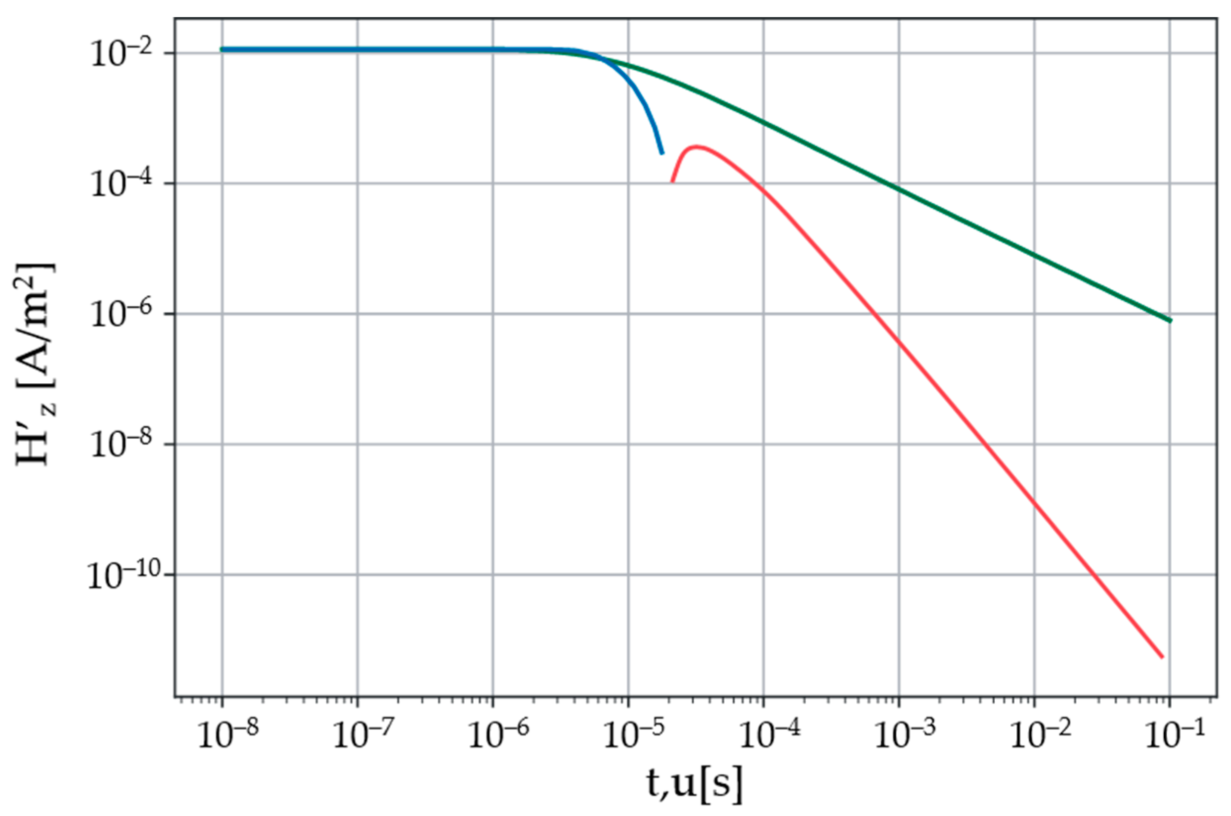
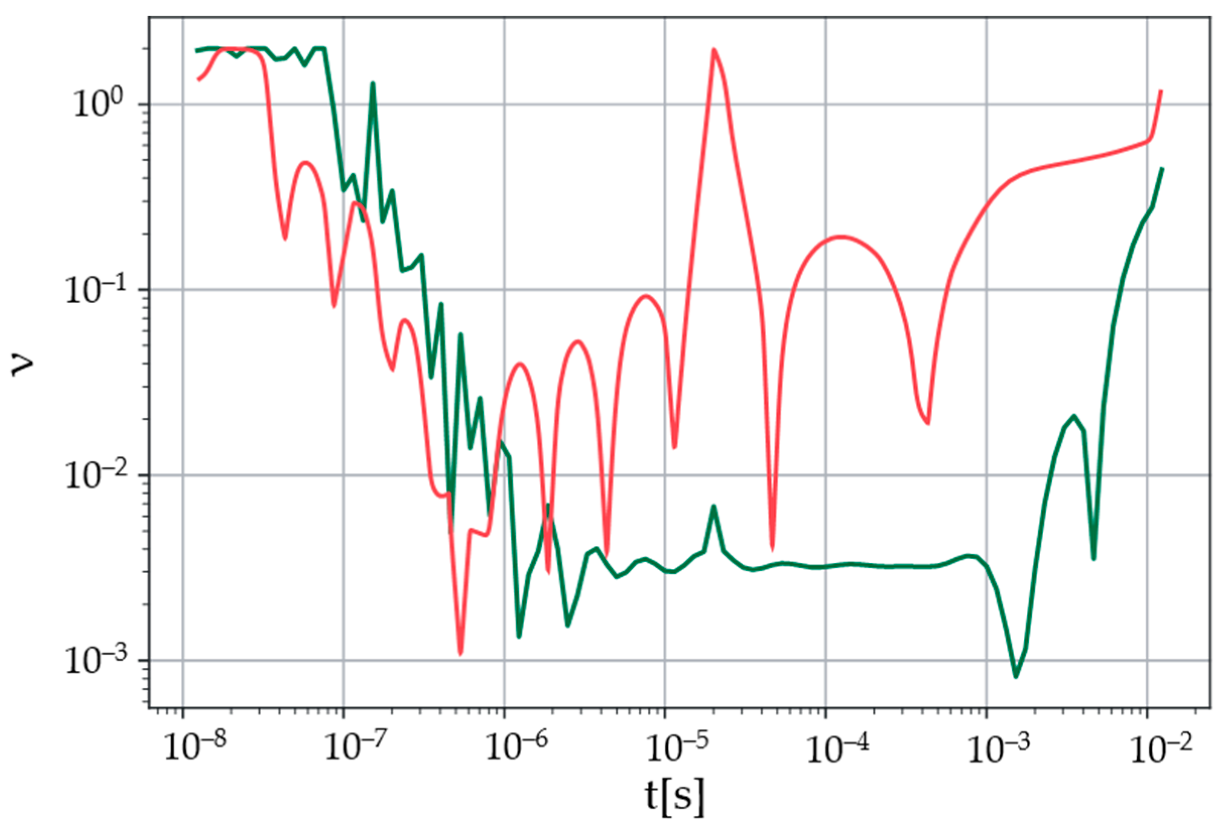
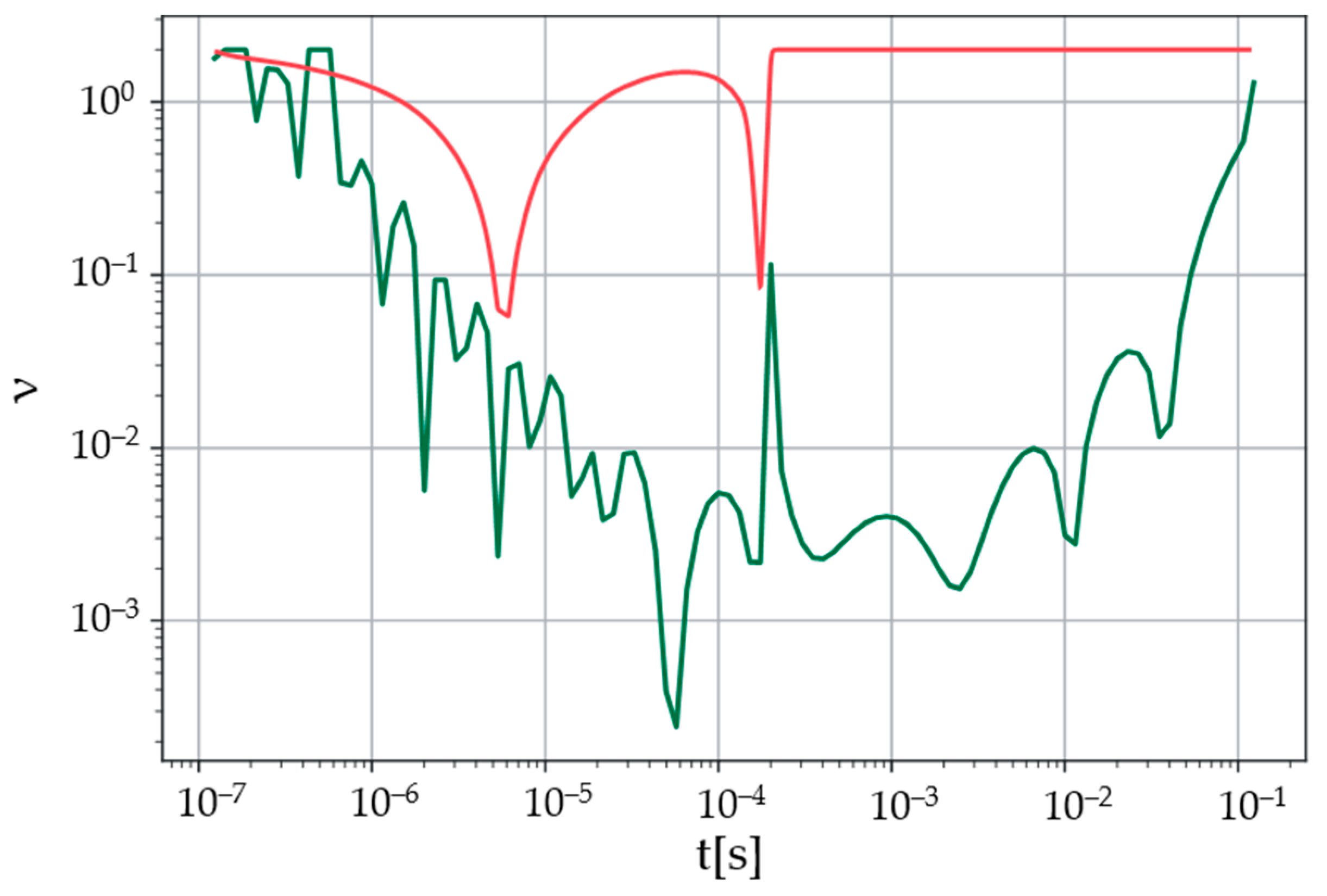
2.4. Features of Numerical Inverse Sumudu Transform for TEM Signals

As consistent with the initial conditions (22) and (23), at $t=0$ the EMF induced in the receiver loop is equal to zero. With allowance for this and the limiting property (2), we set the elements of the vectors $f$ and $g$ with index 0 equal to zero, since they correspond to the values of the EMF at $t=0$ and the Sumudu images of the EMF at $u=0$. Based on this, from system (27) we exclude the vector element of unknowns $f^0$ and the first equation. As a result, we acquire a modified system:

$$\frac{K(u^i,t^1)}{2}{t}^1+{\sum }_{j=1}^{j=n-1}\frac{K(u^i,t^{j+1})f^{j+1}+K(u^i,t^j)f^j}{2}(t^{j+1}-t^j)=g^{j}i=1,2,\dots ,n.$$

(34)

Further on, by the system of equations $Kf=g$ we mean the modified system (34).

As far as the integration region $[0,b]$ contains drastically different-scale $t$ values, the $t^i$ and $u^i$ points used to discretize the integral Equation (25) are specified using the following relation:

$$t^i=u^i=t^i(h{)}^{i-1},i=1,2,\dots n,$$

(35)

where

$$h={\left(\frac{b}{t^1}\right)}^{\frac{1}{n-1}}.$$

The $t^1$ and $b$ values are selected depending on the expected properties of the time-dependent EMF induced in the receiver loop.

As described in [79], the absolute values of the EMF induced in the receiver loop can differ by more than 6 orders of magnitude over time. Accordingly, different elements of the $f_{\alpha }$ vector will differ just as much. Therefore, choosing the identity matrix as the regularizing $R$ does not provide a satisfactory result. This is because the elements of the $f_{\alpha }$ vector, corresponding to the values of the sought-for function at late times after turning on the current in the source, do not have a significant effect when calculating the second term in (29) compared to those associated with the function values at early times. In order for the second term in (29) to have sufficient sensitivity to all elements of the $f_{\alpha }$ vector, the diagonal matrix $R_q$ is to be used as the matrix $R$, the diagonal elements being specified in the following manner:

$$[R{]}_{i,i}=(t^i{)}^q,i=1,2,\dots ,n,$$

where $q$ is a parameter. An increase in the parameter $q$ leads to a sensitivity growth of the second term in (29) to the values of the sought-for function at late times. Along with this, the sensitivity to the function values at early times deteriorates. Determining the value of $q$ requires keeping the sensitivity balance at all times.

Thus, an approximate inverse transformation for the Sumudu image of the EMF can be performed through the following expression:

$$f_{\alpha ,q}={\left(K^{T}K+\alpha R_q^T{R}_q\right)}^{-1}{K}^{T}g.$$

(36)

To specify a pair of the parameters $\alpha$ and $q$, we draw on the idea of choosing the optimal (in some sense) preconditioning matrix in the simple iteration method. In this case, the preconditioning matrix will depend on as many as two parameters—$\alpha$ and $q$:

$$P_{\alpha ,q}={\left(K^{T}K+\alpha R_q^T{R}_q\right)}^{-1}{K}^T.$$

When inverting the Sumudu image of the EMF, the direct use of the quasi-optimal criterion for choosing the parameter $\alpha$ also encounters difficulties. They are associated with various scales of the elements of the vector $f_{\alpha }$ at different times. The elements of the difference vector (31) are highly different-scale, with the sensitivity of the vector difference norm to the late-time elements being extremely low. To overcome this deficiency, we scale the elements of the difference vector from (31). We define the following function:

$$\phi (\alpha ,q)={\sum }_{i=1}^n{\left(\frac{f_{\alpha ,q}^i-{\tilde{f}}_{\alpha ,q}^i}{|f_{\alpha ,q}^i|+|{\tilde{f}}_{\alpha ,q}^i|}\right)}^2,$$

where

$$f_{\alpha ,q}=P_{\alpha ,q}g,$$

$${\tilde{f}}_{\alpha ,q}=P_{\alpha ,q}K{f}_{\alpha ,q}.$$

As the optimal pair of the parameters ${\alpha }^{*}$ and $q^{*}$ we choose $\alpha >0$ and $q\ge 0$, which provide a minimum of the function $\phi (\alpha ,q)$. We search for an approximate solution to the minimization problem by completely enumerating the values $({\alpha }^i,q^j)$ from the set where elements are given as:

$$({\alpha }^i,q^j)=({\alpha }^0(p{)}^i,q^0+hj),i=0,1,\dots ,k_{\alpha },j=0,1,\dots ,k_q.$$

Note that the above-proposed technique for the approximate solution to the integral Equation (25) can be applied for calculating the inverse Laplace transform of a real function. This function can be either known or obtained through (3) from some Sumudu image. For the inverse Laplace transform to be performed, the Sumudu kernel $K(u,t)=\frac{1}{u}\mathit{exp}(-\frac{t}{u})$ is to be replaced with the Laplace kernel $K(s,t)=\mathit{exp}(-st)$, and the collocation points $u^i$—with $s^i$ according to the formula:

$$s^i=\frac{1}{u^{n-i+1}},i=1,2,\dots ,n.$$

In sum, the inverse Sumudu transformation can be conducted in two ways. The first one is to utilize the above-proposed method directly to the Sumudu image. The second is to apply this method to invert the Laplace image obtained using (3). The computational properties of these two approaches depend on the different spectral properties of the linear system matrices (34) that approximate the kernels of the Sumudu and Laplace transforms.

2.5. Computational Experiment

The use of the Sumudu transform to model TEM signals is illustrated in the following example. The modeling area is divided by a horizontal plane into two half-spaces that are homogeneous in physical properties: the upper half-space is non-conductive air; the lower half-space is a conductive earth. There are circular transmitter and receiver loops located on the Earth’s surface. The current is switched off at time $t=0$. It can be shown that the electric field strength obtained under similar conditions is the fundamental solution in time to problem (21)–(25). Accordingly, its Sumudu image in time satisfies (19) and (20). If the radii of the loops are sufficiently small compared to the distance between their centers, then the transmitter loop can be replaced with a vertical magnetic dipole; the EMF in the receiver coil can be taken to be proportional to the time derivative of the z-component of the magnetic field strength $\frac{\partial H_z(t)}{\partial t}$ at the center of the receiver loop.

For the Laplace image of the function $\frac{\partial H_z(t)}{\partial t}$ there exists an analytic expression [79]:

$$L[\frac{\partial H_z(t)}{\partial t}]=\frac{M}{2\pi {\mu }_0\sigma r^5}(9s^{-1}-(9s^{-1}+9a{s}^{-1/2}+4a^2+a^3{s}^{1/2})\mathit{exp}(-a{s}^{1/2})),$$

(37)

where $a=\sqrt{{\mu }_0\sigma r}$, $\sigma$ is the specific electrical conductivity of the lower half-space, ${\mu }_0$ is the magnetic permeability of vacuum, r is the distance between the centers of the loops, M is the magnetic dipole moment. Through the connection between the Laplace and Sumudu transforms (4), we write the Sumudu image of the function $\frac{\partial H_z(t)}{\partial t}$ as follows:

$$S[\frac{\partial H_z(t)}{\partial t}]=\frac{M}{2\pi {\mu }_0\sigma r^{5}u}(9u-(9u+9a{u}^{1/2}+4a^2+a^3{u}^{-1/2})\mathit{exp}(-a{u}^{-1/2})).$$

(38)

Having performed the analytic inverse Laplace transformation for (37), we obtain the analytic expression for $\frac{\partial H_z(t)}{\partial t}$ [79]:

$$\frac{\partial H_z(t)}{\partial t}=\frac{-M}{2\pi {\mu }_0\sigma r^{5}u}(9\mathit{erf}(\theta r)-2r{\pi }^{-1/2}(9+6{\theta }^2{r}^2+4{\theta }^4{r}^4)\mathit{exp}(-{\theta }^2{r}^2)),$$

(39)

where $\theta =\sqrt{{\mu }_0\sigma /4/t}$, $\mathit{erf}(t)$ is the error function:

$$\mathit{erf}(t)=\frac{2}{\sqrt{\pi }}{\int }_0^t\mathit{exp}(-{\tau }^2)d\tau .$$

Figure 1 gives the function $\frac{\partial H_z(t)}{\partial t}$ and its Sumudu image (38) at r = 100 m, σ = 0.01 S/m. By the example of $\frac{\partial H_z(t)}{\partial t}$ and its Sumudu image, we examine the features of performing the inverse Sumudu transformation for the TEM sounding problem via a numerical solution of the first-type integral Equation (25). The function $\frac{\partial H_z(t)}{\partial t}$ has characteristic properties for the EMF induced in the receiver loop (Figure 1). At small times the function does not change noticeably, but at later times it begins to vary in proportion to $t^{-2.5}$.

Let us focus on the capability of the proposed computational method for the inverse Sumudu transformation of function (38). We define a set of points $t^i$ and $u^i$ through (35). To do this, one is to set the values of the parameters $n$, $b$ and $t^1$. As computational experiments have shown, a fairly accurate result is acquired if the following heuristic rule is employed to set the values of $b$ and $t^1$: $t^1=10^{-6}b$, where b is the point on the time axis for which the relation holds:

$$\underset{\tau }{max}\left|\frac{\partial H_z(\tau )}{\partial \tau }\right|=10^{-8}\left|\frac{\partial H_z(t)}{\partial t}\right|.$$

Finding the value of b requires knowing the function $\frac{\partial H_z(t)}{\partial t}$ in advance. An estimate of this function can be made via the method proposed in the presented research, by setting the value of the parameter b a priori large. The value of the parameter n is further chosen to be equal to 100 in all cases. Having the set of points $t^i$ and $u^i$, we generate the matrix and the right-side vector of linear system (34). To solve this system, we resort to Tikhonov’s regularization method (36). We find the parameters $\alpha$ and $q$ by means of the proposed modification of the quasi-optimal criterion in the following range:

$$(\alpha ,q)\in [1,10^5]\times [0,3].$$

The right-side vector of linear system (28) may be distorted by noise. This may happen when obtaining the elements of this vector from the solution to problem (19)–(20), which was found by grid methods (finite difference, finite element, etc.) or some other approximate methods. To simulate this effect, we modify the elements of the right-side vector $g_0$ without noise:

$$g_{\delta }^i=g_0^i(1+\delta (-1{)}^i),i=1,2,\dots ,n,$$

where $\delta$ is the assigned relative noise level. The noise level of a particular element of the right-side vector depends on the value of the element itself. This is because different elements of the vector have different scales. As a consequence, additive noise will greatly distort individual elements of the vector with little effect on others.

We introduce the relative error function:

$$\nu (t)=\left|\frac{f_{\delta }(t)-f(t)}{f(t)}\right|,$$

where $f(t)$ is the exact function, $f_{\delta }(t)$ is an approximation of the function $f(t)$.

Now, move on to the influence of the noise level $\delta$ in the Sumudu image (38) on the relative error of inverting the Sumudu image with the proposed method. Figure 2 illustrates the dependence of the relative error $\nu (t)$ on time and on noise level for TEM signals at a distance between the loops of 100 m and the lower half-space conductivity of 0.1 S/m. As previously noted, the proposed method for conducting the inverse Sumudu transformation, with minor modifications, can be applied to invert a real-valued Laplace image. Let us use this fact to obtain an approximation of function (39) from the Laplace image (37). Figure 3 shows the relative errors $\nu (t)$ for the noise level $\delta =0$ and $\delta =10^{-2}$ in the Laplace image (37) at a distance between the loops of 100 m and conductivity of the lower half-space of 0.1 S/m.

As it appears from the figures, the relative error in calculating the inverse Sumudu and Laplace transformations through the proposed method directly depends on the noise level in the original image. The lower the noise level, the smaller the error of the reconstructed function. Moreover, if the noise level is not very high, then more accurate results are obtained by inverting the Laplace transform. However, at a sufficiently high noise level, inverting the Laplace transform does not allow achieving a satisfactory result. The high level of relative error in the reconstructed functions at early times is associated with oscillations of these functions around the exact value. In order to solve the inverse problem of TEM sounding, the EMF values are required at later times—at which the level of the relative error (depending on the noise level) takes acceptable values.

Thus, to calculate the inverse Sumudu transformation by the proposed method at low noise levels in the Sumudu image, one should use the connection between the images of the Laplace and Sumudu transforms, obtain the Laplace image and invert it. In contrast, at sufficiently high noise levels it is necessary to apply the proposed method directly to invert the Sumudu transform.

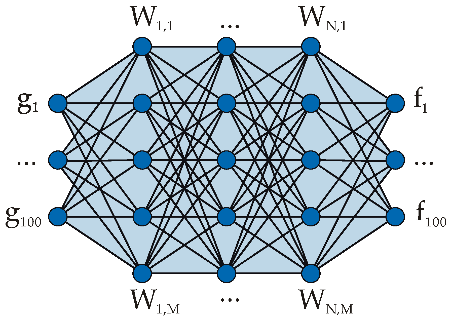
2.6. Neural Network Algorithm Development

A neural network algorithm is created with the help of supervised learning. During the first stage, we acquire a data set with training examples, each representing a pair “function $f(t)$”—“Sumudu image $g\left(u\right)=S[f(t)]$”. This data set has been generated drawing on mathematical modeling for characteristic geoelectric situations and sounding systems. The functions and their images have the form of value vectors at predetermined points $t_i=u_i$.

The acquired data pairs are then normalized by multiplying by $\frac{1}{\mathrm{m}\mathrm{a}\mathrm{x}(g\left(u\right))}$. Such a transformation ensures the exclusion of the sounding system parameters: current strength, loop radii, number of winding turns, etc.

The training set is extended by data augmentation: extra data are created from existing ones by way of simple transformations not requiring substantial computational power. Augmentation increases both data volume and diversity. As far as this technique facilitates recognizing data patterns, it is effective for reducing overfitting of machine learning models [80]. Owing to the linearity property of the Sumudu transform, from two data pairs $\left(g_1,f_1\right),(g_2,f_2)$ we can get a third one as their linear combination:

$$g_3=a{·g}_1+b{·g}_2,$$

$$f_3=a{·f}_1+b{·f}_2,$$

where a and b are constants. The resulting data have to be scaled in the same manner.

In order for the stability of the algorithm to increase, we add normally distributed noise to the input data $g(u)$. The root-mean-square deviation of the noise holds proportion to the signal level and is equal to 5%, which matches with the expected measurement accuracy of the sounding system.

In TEM exploration, the relative change in the signal appears to be more important than its absolute value. This is why we turn to training data transformation: it distorts input and output data spaces for more efficient ANN training. To recapture the required signal dimension, post-processing is applied to the ANN calculation result.

To control the neural network learning (to deter overfitting), the resulting data set (pairs “Sumudu image $g(u)$”—“function $f(t)$”) is separated into two subsamples: 75% directly for training (“training data”) and 25% for control (“test data”).

The inverse Sumudu transform algorithm is accomplished on the basis of ANNs—a class of universally approximating mathematical models [81,82]. In a generic form, an ANN is an arbitrary function of input arguments and internal parameters fitted during the learning process:

$$F\left(g,W\right)=\left\{f_1\left(g,W\right),\dots ,f_n\left(g,W\right)\right\},$$

where $g=\left\{g_1,\dots ,g_n\right\}$ are the input arguments represented by the Sumudu-image vector values; W are the internal parameters of the ANN, which are searched while training; $f_1,\dots ,f_n$ is the set of functions approximating the vector of the inverse Sumudu transform; n is the number of elements in the input and output vectors.

So, the ANN consisting of a combination of linear and nonlinear operations approximates the inverse Sumudu transform by converting the Sumudu images of the functions into their original form. At each training iteration, the neural network result is checked against the known mathematical modeling result.

The architecture of the developed ANN (Figure 4) is a multilayer perceptron (fully connected neural network). First, there is an input layer with a vector of 100 elements (Sumudu image of the function). Also, there are N hidden layers, each with M neurons accompanied by the nonlinear operation ReLu (“rectified linear unit”). And, finally, the output layer where the vector is finally formed—the result of the inverse Sumudu transform (also of 100 elements). The ultimate version of the ANN architecture encompasses 4 hidden layers of 64 neurons.

The weight coefficients of neurons in the ANN layers are initially set at random fashion and then fitted in the process of training. In the present case, estimating the optimal parameters of the ANN is a supervised learning task, which is addressed with the backpropagation algorithm. The ANN training is fulfilled in mini-batch mode with the Adam algorithm—a modification of stochastic gradient descent with the adaptive first-order and second-order momentum estimates [83]. The cost function minimized during the training is the mean absolute error (MAE). This function, coupled with the technique of preprocessing data from the training set enables minimizing the relative deviation between the ANN calculation result and true sounding curves. For the learning efficiency to improve, we practice a sequential decrease in the nominal step of gradient descent (learning rate) depending on its iteration number.

The architecture of the ANN is finally selected subsequent to the results of numerical experiments. The total training time is 40 min (the number of epochs is 2000, Figure 5). The algorithm is trained via parallel computing on the GPU RTX 2080 graphics accelerator.

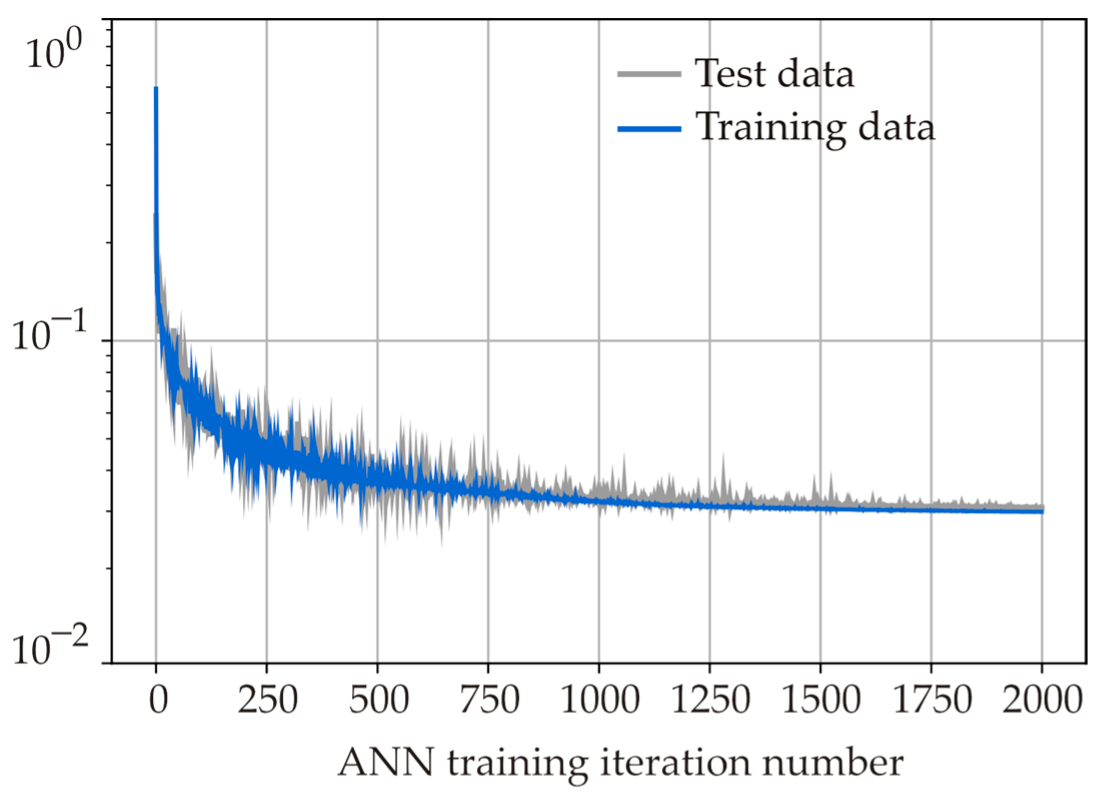
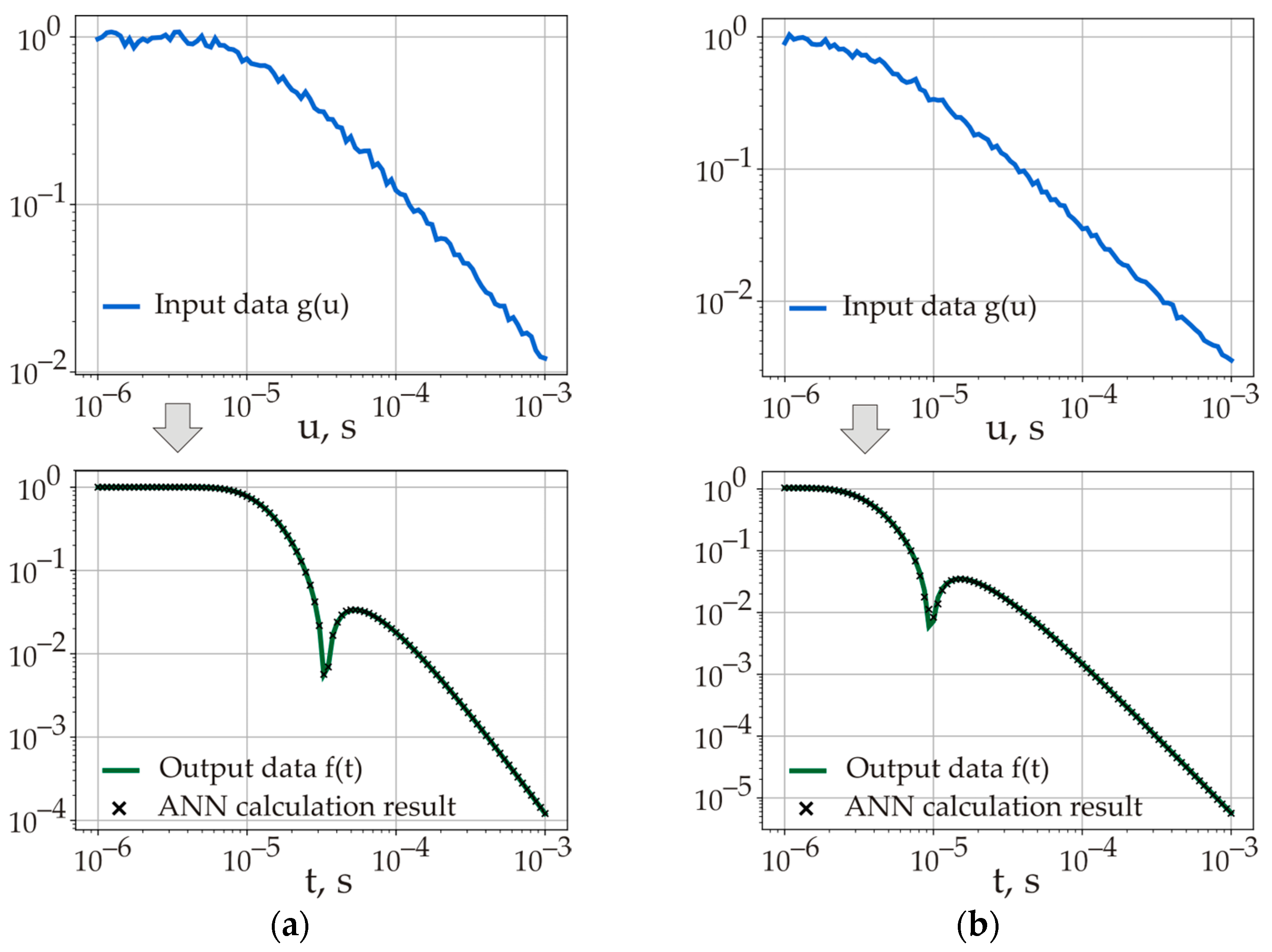
2.7. Neural Network Algorithm: Results and Discusion

After obtaining the optimal values of the weight coefficients, the trained ANN can be used for the inverse Sumudu transform. The neural network algorithm is tested on an additional set of data that are not involved in the ANN training (Figure 6).

Near the zero transition point of the signal to be reconstructed (characteristic minimum in the middle of the time axis), the relative error occasionally increases as opposed to the other time intervals. This is because the absolute value of the first logarithmic derivative of the given function seems to exceed those at the other time intervals.

Table 1. Results of evaluating the algorithmic performance.

Cost Function	Result (Training Data)	Result (Test Data)
Mean absolute error	1.6·10−3	1.8·10−3
Mean squared error	1.4·10−5	2.0·10−5

gives the results of evaluating the algorithmic performance on the training and test data.

As is seen from the data analyzed, our neural network algorithm allows for the inverse Sumudu transform with high accuracy, reasonably good for tackling practical issues. It is significant that when solving first-kind integral equations by traditional methods, the characteristic error in the resulting solution is found to be significantly higher owing to the ill-conditioning [77].

Performance assessment for the algorithm concerned is performed on the central processor CPU Intel i7-8700 (scrutinizing the time needed for the inverse transformation of one Sumudu image). The computing time of the neural network algorithm averaged over ten thousand runs is 2.9·10⁻² s, whereas that of the numerical algorithm [66] equals to 9.3 s. The neural network calculations can also be made in batch mode, making possible efficient parallel computations on multi-processor devices.

To recap, the developed high-performance neural network algorithm exhibits a higher operation speed (320 times faster than the numerical algorithm) with lower resource intensity. In view of the attained transform accuracy, the algorithm is to be implemented into software for modeling TEM signals.

3. Numerical Simulation of TEM Permafrost Monitoring

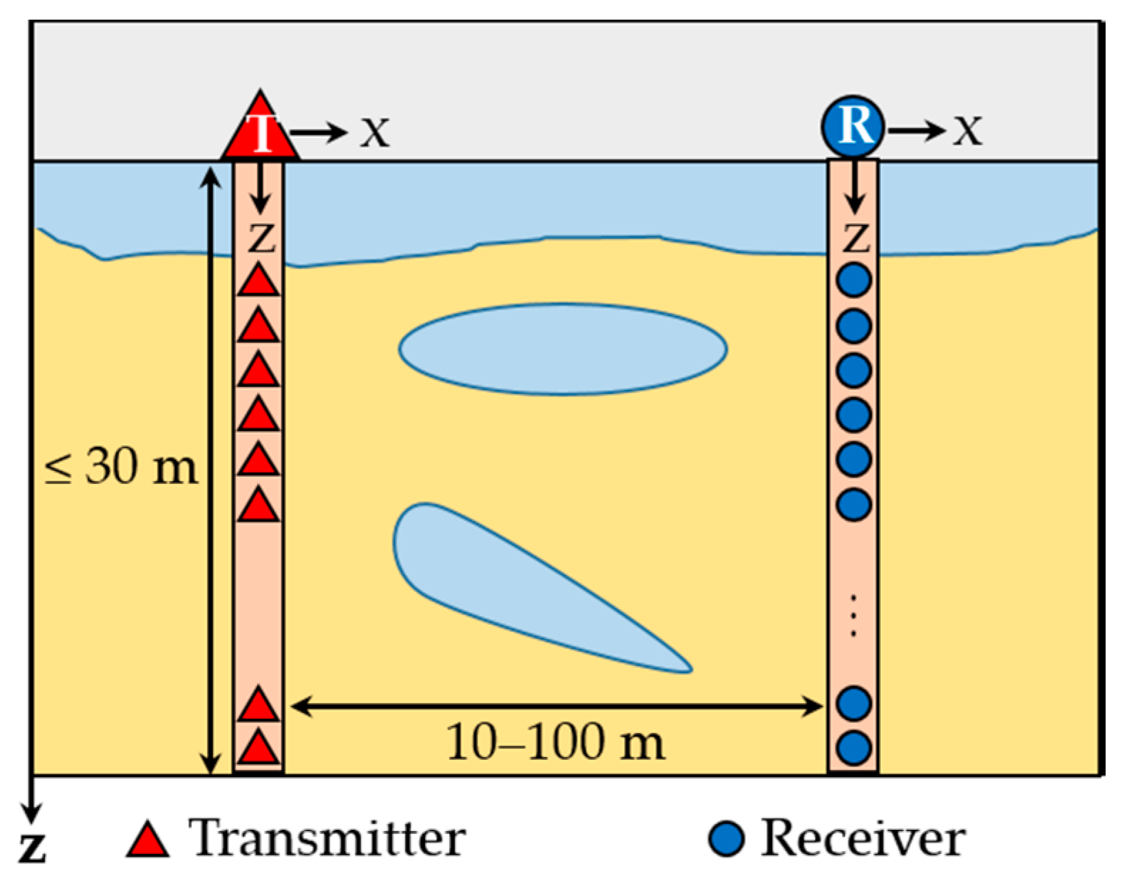
3.1. Cross-Borehole Measurement System

The measurement system for TEM monitoring of the cryolithozone consists of sets of electromagnetic field transmitters and receivers mounted on non-conductive housings and placed in two boreholes (one with transmitters, the other with receivers), Figure 7. The boreholes are situated at the minimum possible distance (10–100 m) from each other so that, on one hand, the sensitivity of the measured signals to the target (thawed) object is highest and, on the other hand, this object is located between the boreholes. Typical borehole depth—up to 30 m. The signal transmitters and receivers are induction coils (antennas) oriented along the axes of a rectangular coordinate system. During the monitoring process, one analyzes the time dependences of the EMF or magnetic field components.

The distinctive features and advantages of the proposed TEM monitoring system are as follows. Firstly, the depth of investigation is not inferior to electrical tomography and is significantly greater than that of ground penetrating radar. Secondly, there is no need to ground the current electrodes, which can pose significant difficulties for the electrical tomography method in the vicinity of industrial facilities. Thirdly, in TEM sounding, measurements occur over a wide time range, which provides a significant amount of geophysical information about the Earth’s interior. Fourthly, the proposed system of TEM cross-borehole exploration is stationary, which reduces the cost of observation system deployment before each subsequent measurement. In addition, in TEM surveys, compared to frequency sounding, there is no need to apply correction for the direct field. The mentioned practical advantages predetermine the prospects of TEM sounding with regard to permafrost monitoring.

To analyze the sensitivity of the signals to geoelectric parameters of the earth, we utilize logarithmic derivatives of the signals. Such derivatives show the relative rate of change in the signal when some parameter is varied. With their help, the relative error in assessing the parameter for a given measurement error is estimated in a linear approximation:

$$\mathsf{\delta }=\frac{{\mathsf{\Delta }}_f}{\left|\frac{\mathit{df}}{\mathit{dp}}(p_0){·p}_0\right|}·100\%,$$

where ${∆}_f=\left|f\right|·f^r+f^a$ is the total absolute measurement error; f is the TEM signal; $f^r$ and $f^a$ are its relative and absolute errors; $p_0$ is the value of the estimated parameter, e.g., the depth of the boundary between thawed and frozen rocks.

The values of the relative and absolute measurement errors are the following: $f^r=0.02$, $f^a=10\mathrm{nV}$, at this the product of the moments of the transmitter and receiver coils is 100 A·m⁴.

To study the dependence of the measured signals on the inter-borehole distance, we have conducted numerical simulation of the error in tracking the freezing depth of the upper part of the section (Figure 8). The observation system comprises the electromagnetic field transmitter and receiver located in two boreholes at a fixed depth of 1.5 m, at a distance of 10, 30 and 100 m from each other. Color in Figure 8 indicates the calculated errors in tracing the boundary between thawed and frozen rocks as function of time and the boundary’s vertical depth for different field components: ZZ, YY, XX and XZ (the letters indicate the direction of the magnetic moment of the transmitter and receiver coils along the coordinate axes respectively). The position of the boundary varies from 0 to 2 m.

The dynamic pattern in the error depending on the transmitter-receiver distance has been established. For instance, at the distance L = 10 m the smallest error is observed within the entire depth of the section, not exceeding the permissible limit (up to 10%). Near the transmitter at a depth of about 1.5 m, the error for the YY and ZZ components does not exceed 1%. The error gradually increases to 100% and higher with the growing inter-borehole distance and growing recording time. For L = 30 m, the error differs slightly from the case of L = 10 m; a good result is evidenced for all the measured field components. As L increases to 100 m, there is a noticeable narrowing of the range of permissible measurement errors. This being the case, for the ZZ and YY components below the source depth (1.5 m) the error rises by an order of magnitude; for the XX and XZ components, the range of adequate error values becomes too narrow for a rigorous analysis of the EMF signals. Nevertheless, for the components ZZ and YY, even at such a large distance L = 100 m, it is possible to trace the thawing boundary.

Hence, the scrutinized error varies depending on both the distance between the transmitter and receiver, and on the field component (ZZ, YY, XX or XZ). The smallest measurement error is observed when applying the ZZ and YY components, which leads to the conclusion that it is for these components that the boundary of the thawing layer will be traced most reliably.

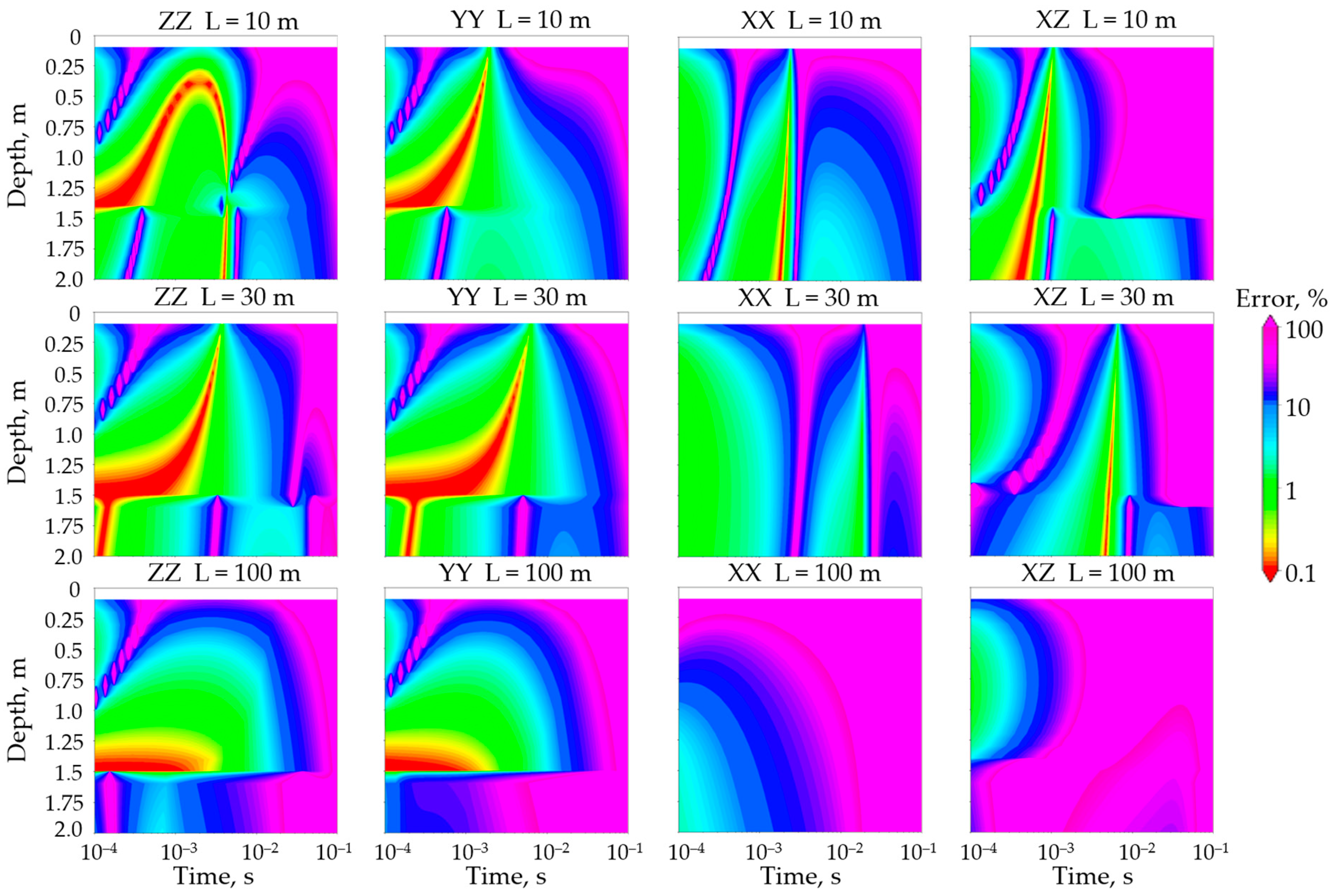
3.2. Simulation Results on Monitoring Real Objects

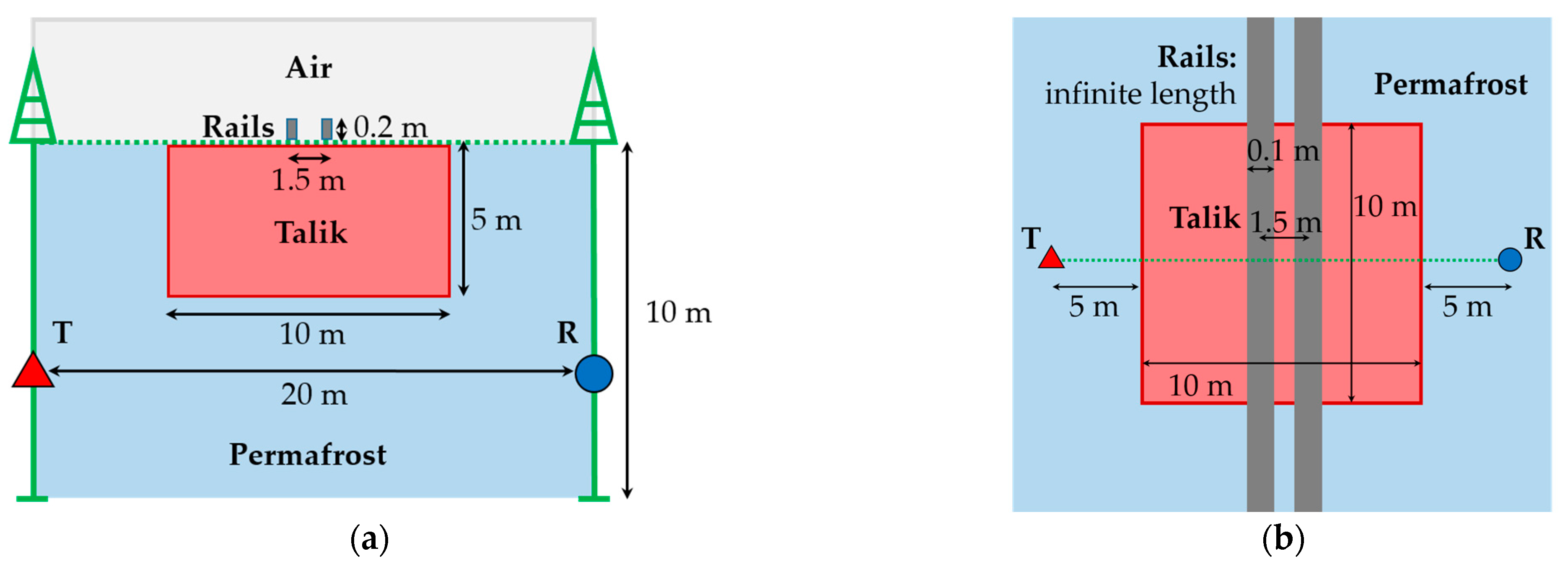
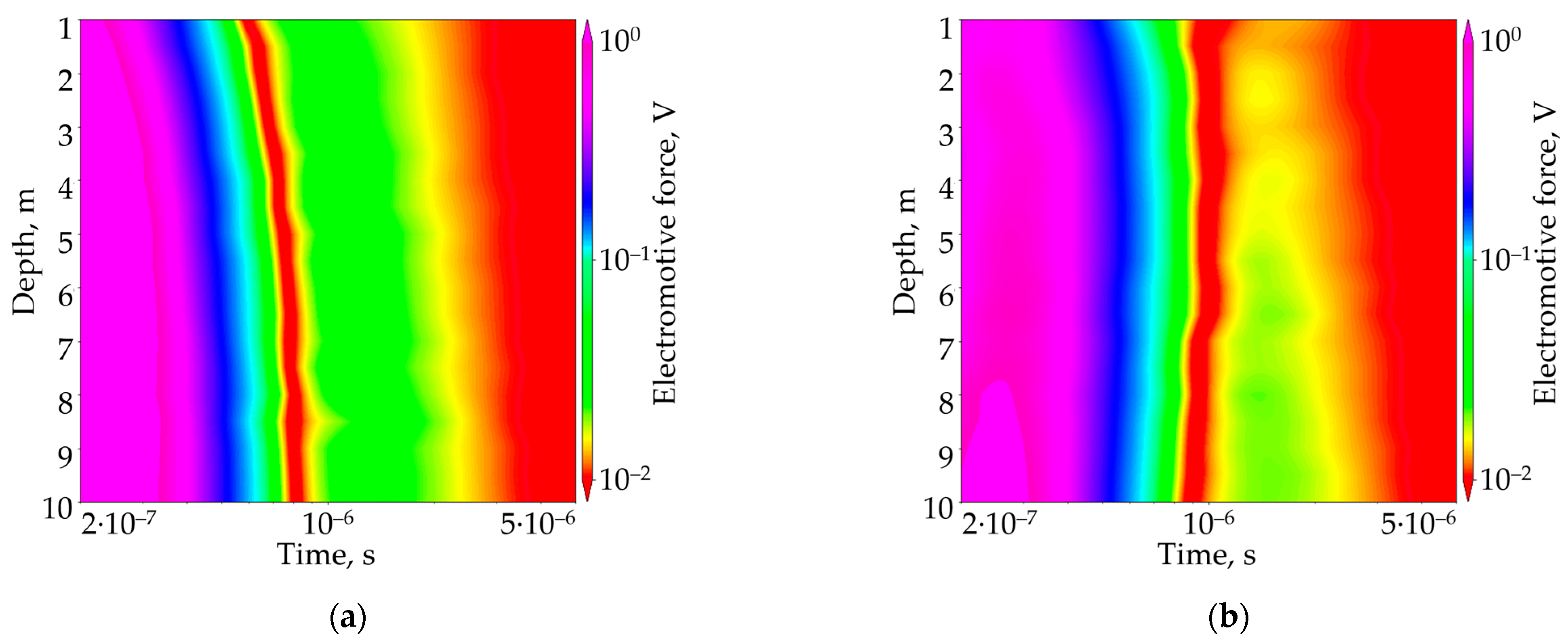
3.2.1. Railway in Yakutia

A realistic geoelectric model of the railway in Yakutia (Figure 9) includes host permafrost rocks with resistivity ${\rho }_0=200$ ohm·m (lower half-space) and air with resistivity ${\rho }_{air}={10}^6$ ohm·m (upper half-space). On the Earth’s surface there are metal rails of infinite length (the optimal length is chosen for calculations) with a height of 0.2 m and a width of 0.1 m; the distance between the centers of the rails is 1.5 m; the metal resistivity ${\rho }_{met}=0.01$ ohm·m. Directly under the rails, there is an open talik formed in the shape of a rectangular parallelepiped with resistivity ${\rho }_{tal}=50$ ohm·m, its height being 5 m and width 10 m. In the frozen host rocks, the polarization parameters are taken into account; resistivity in the frequency domain is described by Pelton’s formula [84]:

$$\rho \left(\omega \right)={\rho }_0\left(1-m\left(1-\frac{1}{1+{\left(i\omega \tau \right)}^c}\right)\right),$$

where ${\rho }_0$ is the direct current resistivity, m is the polarizability, c is the exponent, and τ is the relaxation time. For the simulation we take: ${\rho }_0=200$ ohm·m, m = 0.3, τ = 10⁻⁴ s, c = 1.

The cross-borehole distance is 20 m, the depth of two boreholes is 10 m. The transmitters and receivers are located at equal depths in the two boreholes—from 1 m to 10 m with 0.5 m step. The boreholes are centrally arranged relative to the open talik.

The TEM signals are computed in the reference medium of 200 ohm·m with the rails: without the talik and with it (Figure 10).

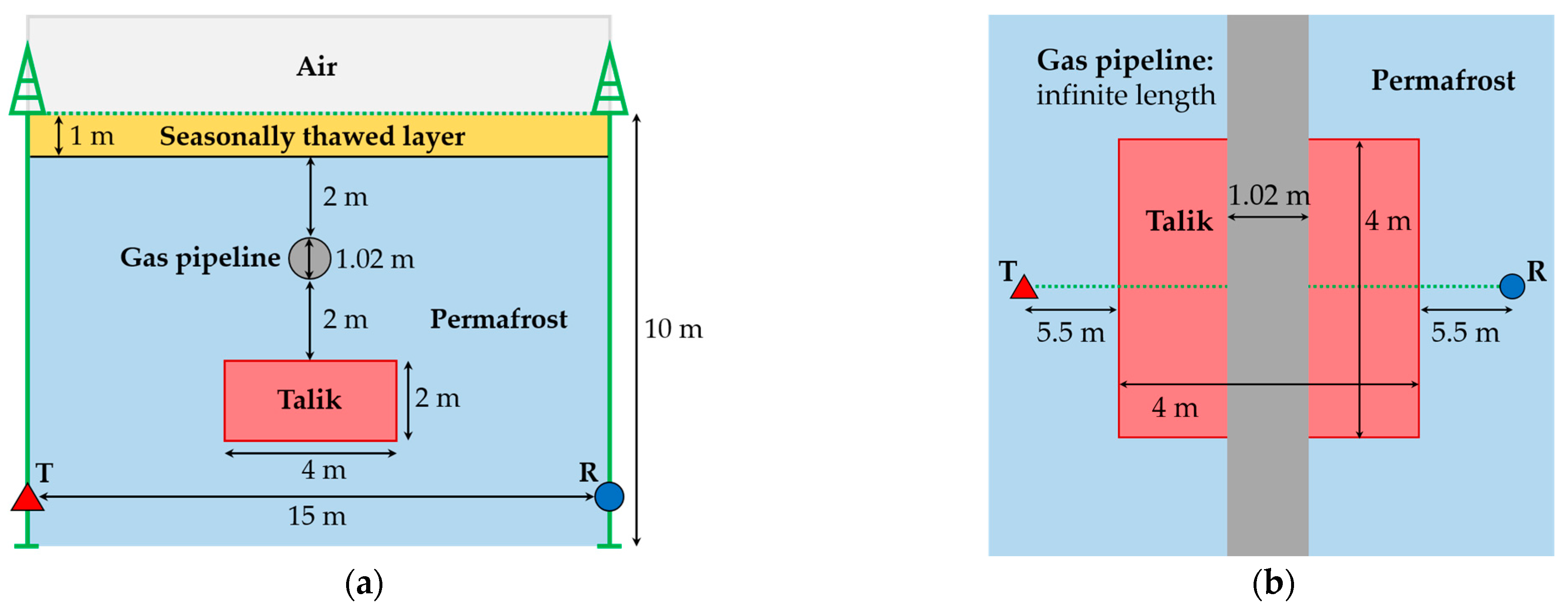
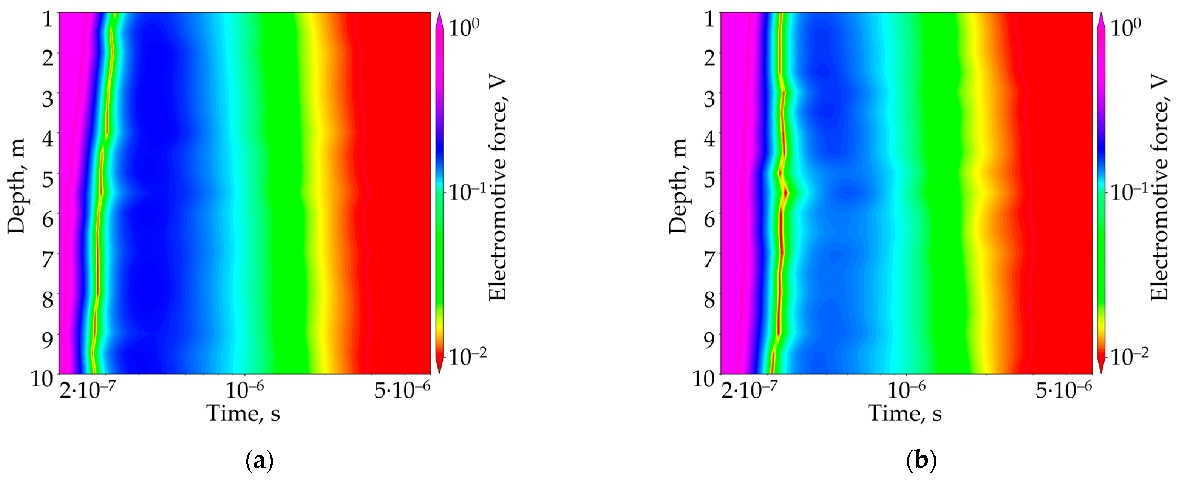
3.2.2. Underground Gas Transmission Pipeline on the Gyda Peninsula

A realistic geoelectric model of the underground gas transmission pipeline on the Gyda Peninsula (Figure 11) comprises permafrost rocks with resistivity ${\rho }_0=500$ ohm·m and air above the Earth’s surface with resistivity ${\rho }_{air}={10}^6$ ohm·m. At a depth of up to 1 m below the surface there is a seasonally thawed layer with resistivity ${\rho }_{stl}=50$ ohm·m. Then, there is a two-meter-thick layer of frozen rock (${\rho }_0=500$ ohm·m), after which lies a gas pipeline of infinite length (the optimal length is chosen for calculations) with an outer diameter of 1.02 m and metal wall thickness of 0.032 m; metal resistivity is 0.01 ohm·m. The resistivity of the gas in the pipeline ${\rho }_{gas}={10}^6$ ohm·m. Further in depth, 2 m below the gas pipeline, there is a closed talik formed in the shape of a rectangular parallelepiped: a resistivity of 10 ohm·m and dimensions of 2 m × 4 m × 4 m (where 2 m is the height of the talik). The talik is located symmetrically relative to the axis of the gas pipeline. Parameters of the Pelton formula for the frozen host rocks with ${\rho }_0=500$ ohm·m: m = 0.5; τ = 2·10⁻⁴ s; c = 1.

The inter-borehole distance is 15 m, the depth of the borehole is 10 m. The transmitters and receivers are at equal depths in the two boreholes—from 1 m to 10 m with a step of 0.5 m. The inter-borehole axis passes through the center of the closed talik, perpendicular to the gas pipeline.

The TEM signals are simulated in the reference earth of 500 ohm·m with the seasonally thawed layer and the gas pipeline—without and with the talik (Figure 12).

It follows from the analysis of the results of three-dimensional numerical modeling in realistic geoelectric models of the railway in Yakutia and the underground gas transmission pipeline on the Gyda Peninsula that there is good sensitivity of the TEM monitoring signals to the conductive talik at early and middle times of 10⁻⁵–5·10⁻⁶ s. In potentially hazardous areas, it is advisable to place the monitoring boreholes at least every 5 m in order to promptly detect changes in geocryological properties in the vicinity of a target object. Visual analysis of the TEM signals does not provide an insight into the size and location of a thawed zone, for which reason data inversion has to be used to determine its parameters.

4. Conclusions

A novel technique of cross-borehole transient electromagnetic permafrost monitoring is considered. We have created an original algorithm for fast three-dimensional modeling of TEM signals, which is based on a combination of the vector finite element method, the Sumudu integral transform and artificial neural networks. In relation to modeling electromagnetic fields, this approach has been implemented in world practice for the first time.

The proposed method for calculating the inverse Sumudu transform, focused on Sumudu images, is applicable to obtain the time dependence of the electromotive force induced in the receiver loop in a practically significant time range. This enables using the Sumudu transform to solve practical problems and makes it a direct alternative to the Laplace and Fourier transforms. Due to the fact that the Sumudu transform allows calculations in the field of real numbers only, significant savings in computational resources are achieved when modeling in complex geometric and physical areas.

A disadvantage of the Sumudu transform is the lack of an explicit formula for obtaining its inverse transformation, which is why we have examined the capability of applying an artificial neural network to create an inverse Sumudu transform algorithm for the problem of transient electromagnetic sounding. Through parallel computing on a graphics accelerator, an artificial neural network with a multilayer perceptron architecture has been trained. The high accuracy of inverting Sumudu images of functions in the presence of noise has been demonstrated, which is challenging when solving first-kind integral equations by conventional methods due to their poor conditionality. We have established the developed algorithm to be characterized by a higher performance (on average, more than 300 times) in comparison with the numerical solution, with a significantly lower resource intensity.

Numerical modeling of the TEM signals and their logarithmic derivatives with respect to geoelectric model parameters has been carried out. A sensitivity analysis of the signals to the boundary between frozen and thawed rocks shows that the inter-borehole distance at which an acceptable signal level is maintained can reach 100 m, the smallest error in tracking the position of the boundary being observed when using the ZZ and YY components. The formation of a talik is significantly manifested in the recorded transient electromagnetic responses, which makes it possible to prevent a potential environmental threat. At the same time, a visual analysis of changes in TEM signals during the monitoring process does not provide an idea of the size and location of a thawed zone. Therefore, to evaluate its parameters numerically, data inversion seems to be necessary. The first experience in creating such an inversion algorithm has already been gained [85]. In the future, the algorithm will be elaborated: we are intending to consider a wide range of realistic geoelectric models and case studies with permafrost under the foundations of civil and industrial facilities.

References

1. Smith, S.L.; O’Neill, H.B.; Isaksen, K.; Noetzli, J.; Romanovsky, V.E. The changing thermal state of permafrost. Nat. Rev. Earth Environ. 2022, 3, 10–23. [Google Scholar] [CrossRef]
2. Miner, K.R.; Turetsky, M.R.; Malina, E.; Bartsch, A.; Tamminen, J.; McGuire, A.D.; Fix, A.; Sweeney, C.; Elder, C.D.; Miller, C.E. Permafrost carbon emissions in a changing Arctic. Nat. Rev. Earth Environ. 2022, 3, 55–67. [Google Scholar] [CrossRef]
3. Nitzbon, J.; Westermann, S.; Langer, M.; Martin, L.C.P.; Strauss, J.; Laboor, S.; Boike, J. Fast response of cold ice-rich permafrost in northeast Siberia to a warming climate. Nat. Commun. 2020, 11, 2201. [Google Scholar] [CrossRef]
4. Hjort, J.; Karjalainen, O.; Aalto, J.; Westermann, S.; Romanovsky, V.E.; Nelson, F.E.; Etzelmüller, B.; Luoto, M. Degrading permafrost puts Arctic infrastructure at risk by mid-century. Nat. Commun. 2018, 9, 5147. [Google Scholar] [CrossRef]
5. Hjort, J.; Streletskiy, D.; Doré, G.; Wu, Q.; Bjella, K.; Luoto, M. Impacts of permafrost degradation on infrastructure. Nat. Rev. Earth Environ. 2022, 3, 24–38. [Google Scholar] [CrossRef]
6. Streletskiy, D.A.; Clemens, S.; Lanckman, J.-P.; Shiklomanov, N.I. The costs of Arctic infrastructure damages due to permafrost degradation. Environ. Res. Lett. 2023, 18, 015006. [Google Scholar] [CrossRef]
7. Langer, M.; von Deimling, T.S.; Westermann, S.; Rolph, R.; Rutte, R.; Antonova, S.; Rachold, V.; Schultz, M.; Oehme, A.; Grosse, G. Thawing permafrost poses environmental threat to thousands of sites with legacy industrial contamination. Nat. Commun. 2023, 14, 1721. [Google Scholar] [CrossRef] [PubMed]
8. Best, M.; Fage, I.; Ryan, S. Mapping the Distribution of Permafrost using the Resolve Airborne EM System: Klondike Highway, Yukon, Canada. Recorder 2019, 44, 1–12. [Google Scholar]
9. Kaiser, S.; Boike, J.; Grosse, G.; Langer, M. The Potential of UAV Imagery for the Detection of Rapid Permafrost Degradation: Assessing the Impacts on Critical Arctic Infrastructure. Remote Sens. 2022, 14, 6107. [Google Scholar] [CrossRef]
10. Varlamov, S.P. Thermal monitoring of railway subgrade in a region of ice-rich permafrost, Yakutia, Russia. Cold Reg. Sci. Technol. 2018, 155, 184–192. [Google Scholar] [CrossRef]
11. Liu, H.; Huang, S.; Xie, C.; Tian, B.; Chen, M.; Chang, Z. Monitoring Roadbed Stability in Permafrost Area of Qinghai–Tibet Railway by MT-InSAR Technology. Land 2023, 12, 474. [Google Scholar] [CrossRef]
12. Ma, D.; Motagh, M.; Liu, G.; Zhang, R.; Wang, X.; Zhang, B.; Xiang, W.; Yu, B. Thaw Settlement Monitoring and Active Layer Thickness Retrieval Using Time Series COSMO-SkyMed Imagery in Iqaluit Airport. Remote Sens. 2022, 14, 2156. [Google Scholar] [CrossRef]
13. Guo, M.; Lu, Y.; Yu, W.; Xu, L.; Hu, D.; Chen, L. Permafrost change and its engineering effects under climate change and airport construction scenarios in northeast China. Transp. Geotech. 2023, 43, 101117. [Google Scholar] [CrossRef]
14. Feodorov, A.B.; Egorov, A.V.; Pavlova, P.L.; Sviridov, L.I.; Zagorulko, V.N. Analysis of permafrost conditioning in the oil field. J. Phys. Conf. Ser. 2020, 1515, 052070. [Google Scholar] [CrossRef]
15. Vasiliev, G.G.; Dzhaljabov, A.A.; Leonovich, I.A. Analysis of the causes of engineering structures deformations at gas industry facilities in the permafrost zone. J. Min. Inst. 2021, 249, 377–385. [Google Scholar] [CrossRef]
16. Pashilov, M.V. Findings of thermometric monitoring of the top layer of permafrost during hydrocarbon production in the European North of Russia. Arct. Environ. Res. 2018, 18, 53–61. [Google Scholar] [CrossRef]
17. Chuvilin, E.; Tipenko, G.; Bukhanov, B.; Istomin, V.; Pissarenko, D. Simulating Thermal Interaction of Gas Production Wells with Relict Gas Hydrate-Bearing Permafrost. Geosciences 2022, 12, 115. [Google Scholar] [CrossRef]
18. Wang, F.; Li, G.; Ma, W.; Wu, Q.; Serban, M.; Samsonova, V.; Fedorov, A.; Jiang, N.; Wang, B. Pipeline–permafrost interaction monitoring system along the China–Russia crude oil pipeline. Eng. Geol. 2019, 254, 113–125. [Google Scholar] [CrossRef]
19. Varlamov, S.; Skryabin, P.; Zhirkov, A.; Wen, Z. Monitoring the Permafrost Conditions along Pipeline Routes in Central Yakutia, Russia. Land 2022, 11, 2331. [Google Scholar] [CrossRef]
20. Rajendran, S.; Sadooni, F.N.; Al-Kuwari, H.A.S.; Anisimov, O.; Govil, H.; Nasir, S.; Vethamony, P. Monitoring oil spill in Norilsk, Russia using satellite data. Sci. Rep. 2021, 11, 3817. [Google Scholar] [CrossRef]
21. Belash, T.A.; Dymov, E.A. Influence of Tanks Design Features on Earthquake Resistance in Permafrost Areas. IOP Conf. Ser. Earth Environ. Sci. 2022, 988, 042089. [Google Scholar] [CrossRef]
22. Zhao, X.; Wang, J. Numerical Studies of Bridge Foundation Temperature Control Technology in Permafrost Regions. IOP Conf. Ser. Earth Environ. Sci. 2020, 455, 012130. [Google Scholar] [CrossRef]
23. Fedin, K.V.; Olenchenko, V.V.; Osipova, P.S.; Pechenegov, D.A.; Kolesnikov, Y.I.; Ngomayezwe, L. Assessment of the technical condition of bridges and their ground foundations using the electrical resistivity tomography and the passive seismic standing wave method. J. Appl. Geophys. 2023, 217, 105188. [Google Scholar] [CrossRef]
24. Shaidurov, G.Y.; Amelchugov, S.P.; Igolkin, V.I.; Tronin, O.A.; Radaev, V.V. Physical basis of the remote monitoring method of pile foundations of building structures in permafrost areas. J. Phys. Conf. Ser. 2019, 1399, 022052. [Google Scholar] [CrossRef]
25. Hou, X.; Chen, J.; Yang, B.; Wang, J.; Dong, T.; Rui, P.; Mei, Q. Monitoring and simulation of the thermal behavior of cast-in-place pile group foundations in permafrost regions. Cold Reg. Sci. Technol. 2022, 196, 103486. [Google Scholar] [CrossRef]
26. Ye, Y.; Li, L.; Xu, X. Physical and Mechanical Properties of Transmission Line Galloping under the Action of Freezing and Thawing in Variable Temperature Range. Adv. Civ. Eng. 2021, 2021, 8368289. [Google Scholar] [CrossRef]
27. Zhang, J.; Zhou, C.; Zhang, Z.; Melnikov, A.; Jin, D.; Zhang, S. Physical Model Test and Heat Transfer Analysis on Backfilling Construction of Qinghai-Tibet Transmission Line Tower Foundation. Energies 2022, 15, 2329. [Google Scholar] [CrossRef]
28. Bartsch, A.; Strozzi, T.; Nitze, I. Permafrost Monitoring from Space. Surv. Geophys. 2023, 44, 1579–1613. [Google Scholar] [CrossRef]
29. de la Barreda-Bautista, B.; Boyd, D.S.; Ledger, M.; Siewert, M.B.; Chandler, C.; Bradley, A.V.; Gee, D.; Large, D.J.; Olofsson, J.; Sowter, A.; et al. Towards a Monitoring Approach for Understanding Permafrost Degradation and Linked Subsidence in Arctic Peatlands. Remote Sens. 2022, 14, 444. [Google Scholar] [CrossRef]
30. Fraser, R.H.; Leblanc, S.G.; Prevost, C.; van der Sluijs, J. Towards precise drone-based measurement of elevation change in permafrost terrain experiencing thaw and thermokarst. Drone Syst. Appl. 2022, 10, 406–426. [Google Scholar] [CrossRef]
31. Zhang, P.; Chen, Y.; Ran, Y.; Chen, Y. Permafrost Early Deformation Signals before the Norilsk Oil Tank Collapse in Russia. Remote Sens. 2022, 14, 5036. [Google Scholar] [CrossRef]
32. Cheng, F.; Lindsey, N.J.; Sobolevskaia, V.; Dou, S.; Freifeld, B.; Wood, T.; James, S.R.; Wagner, A.M.; Ajo-Franklin, J.B. Watching the Cryosphere thaw: Seismic monitoring of permafrost degradation using distributed acoustic sensing during a controlled heating experiment. Geophys. Res. Lett. 2022, 49, e2021GL097195. [Google Scholar] [CrossRef]
33. Lebedev, M.; Dorokhin, K. Application of Cross-Hole Tomography for Assessment of Soil Stabilization by Grout Injection. Geosciences 2019, 9, 399. [Google Scholar] [CrossRef]
34. Tomassi, A.; Milli, S.; Tentori, D. Synthetic seismic forward modeling of a high-frequency depositional sequence: The example of the Tiber depositional sequence (Central Italy). Mar. Pet. Geol. 2024, 160, 106624. [Google Scholar] [CrossRef]
35. Konstantinov, P.; Zhelezniak, M.; Basharin, N.; Misailov, I.; Andreeva, V. Establishment of Permafrost Thermal Monitoring Sites in East Siberia. Land 2020, 9, 476. [Google Scholar] [CrossRef]
36. Noetzli, J.; Arenson, L.U.; Bast, A.; Beutel, J.; Delaloye, R.; Farinotti, D.; Gruber, S.; Gubler, H.; Haeberli, W.; Hasler, A.; et al. Best Practice for Measuring Permafrost Temperature in Boreholes Based on the Experience in the Swiss Alps. Front. Earth Sci. 2021, 9, 607875. [Google Scholar] [CrossRef]
37. Isaksen, K.; Lutz, J.; Sørensen, A.M.; Godøy, Ø.; Ferrighi, L.; Eastwood, S.; Aaboe, S. Advances in operational permafrost monitoring on Svalbard and in Norway. Environ. Res. Lett. 2022, 17, 095012. [Google Scholar] [CrossRef]
38. Zhang, J.; Revil, A. Cross-well 4-D resistivity tomography localizes the oil–water encroachment front during water flooding. Geophys. J. Int. 2015, 201, 343–354. [Google Scholar] [CrossRef]
39. Commer, M.; Doetsch, J.; Dafflon, B.; Wu, Y.; Daley, T.M.; Hubbard, S.S. Time-lapse 3-D electrical resistance tomography inversion for crosswell monitoring of dissolved and supercritical CO2 flow at two field sites: Escatawpa and Cranfield, Mississippi, USA. Int. J. Greenh. Gas Con. 2016, 49, 297–311. [Google Scholar] [CrossRef]
40. Palacios, A.; Ledo, J.J.; Linde, N.; Luquot, L.; Bellmunt, F.; Folch, A.; Marcuello, A.; Queralt, P.; Pezard, P.A.; Martínez, L.; et al. Time-lapse cross-hole electrical resistivity tomography (CHERT) for monitoring seawater intrusion dynamics in a Mediterranean aquifer. Hydrol. Earth Syst. Sci. 2020, 24, 2121–2139. [Google Scholar] [CrossRef]
41. Herring, T.; Lewkowicz, A.G.; Hauck, C.; Hilbich, C.; Mollaret, C.; Oldenborger, G.A.; Uhlemann, S.; Farzamian, M.; Calmels, F.; Scandroglio, R. Best practices for using electrical resistivity tomography to investigate permafrost. Permafr. Periglac. Process 2023, 34, 494–512. [Google Scholar] [CrossRef]
42. Campbell, S.; Affleck, R.T.; Sinclair, S. Ground-penetrating radar studies of permafrost, periglacial, and near-surface geology at McMurdo Station, Antarctica. Cold Reg. Sci. Technol. 2018, 148, 38–49. [Google Scholar] [CrossRef]
43. Mozaffari, A. Towards 3D Crosshole GPR Full-Waveform Inversion. Ph.D. Thesis, RWTH Aachen University, Aachen, Germany, 2022. [Google Scholar]
44. Pongrac, B.; Gleich, D.; Malajner, M.; Sarjaš, A. Cross-Hole GPR for Soil Moisture Estimation Using Deep Learning. Remote Sens. 2023, 15, 2397. [Google Scholar] [CrossRef]
45. Léger, E.; Saintenoy, A.; Serhir, M.; Costard, F.; Grenier, C. Brief communication: Monitoring active layer dynamics using a lightweight nimble ground-penetrating radar system—A laboratory analogue test case. Cryosphere 2023, 17, 1271–1277. [Google Scholar] [CrossRef]
46. Li, X.; Cao, L.; Cao, H.; Wei, T.; Liu, L.; Yang, X. 2D cross-hole electromagnetic inversion algorithms based on regularization algorithms. J. Geophys. Eng. 2023, 20, 1030–1042. [Google Scholar] [CrossRef]
47. Wang, X.; Shen, J.; Wang, Z. 3D general-measure inversion of crosswell EM data using a direct solver. J. Geophys. Eng. 2021, 18, 124–133. [Google Scholar] [CrossRef]
48. Cao, L.; Li, X.; Cao, H.; Liu, L.; Wei, T.; Yang, X. 3-D Crosswell electromagnetic inversion based on IRLS norm sparse optimization algorithms. J. Appl. Geophys. 2023, 214, 105072. [Google Scholar] [CrossRef]
49. Oldenborger, G.A.; LeBlanc, A.-M. Monitoring changes in unfrozen water content with electrical resistivity surveys in cold continuous permafrost. Geophys. J. Int. 2018, 215, 965–977. [Google Scholar] [CrossRef]
50. Tomaškovičová, S.; Ingeman-Nielsen, T. Quantification of freeze–thaw hysteresis of unfrozen water content and electrical resistivity from time lapse measurements in the active layer and permafrost. Permafr. Periglac. Process. 2023, 34, 1–19. [Google Scholar] [CrossRef]
51. Boaga, J.; Phillips, M.; Noetzli, J.; Haberkorn, A.; Kenner, R.; Bast, A. A Comparison of Frequency Domain Electro-Magnwtometry, Electrical Resistivity Tomography and Borehole Temperatures to Assess the Presence of Ice in a Rock Glacier. Front. Earth Sci. 2020, 8, 586430. [Google Scholar] [CrossRef]
52. Kim, K.; Lee, J.; Ju, H.; Jung, J.Y.; Chae, N.; Chi, J.; Kwon, M.J.; Lee, B.Y.; Wagner, J.; Kim, J.-S. Time-lapse electrical resistivity tomography and ground penetrating radar mapping of the active layer of permafrost across a snow fence in Cambridge Bay, Nunavut Territory, Canada: Correlation interpretation using vegetation and meteorological data. Geosci. J. 2021, 25, 877–890. [Google Scholar] [CrossRef]
53. Buddo, I.; Sharlov, M.; Shelokhov, I.; Misyurkeeva, N.; Seminsky, I.; Selyaev, V.; Agafonov, Y. Applicability of Transient Electromagnetic Surveys to Permafrost Imaging in Arctic West Siberia. Energies 2022, 15, 1816. [Google Scholar] [CrossRef]
54. Yang, G.; Xie, C.; Wu, T.; Wu, X.; Zhang, Y.; Wang, W.; Liu, G. Detection of permafrost in shallow bedrock areas with the opposing coils transient electromagnetic method. Front. Environ. Sci. 2022, 10, 909848. [Google Scholar] [CrossRef]
55. Koshurnikov, A.V. The Principles of Complex Geocryological Geophysical Analysis for Studying Permafrost and Gas Hydrates on the Arctic Shelf of Russia. Moscow Univ. Geol. Bull. 2020, 75, 425–434. [Google Scholar] [CrossRef]
56. Swidinsky, A.; Weiss, C.J. On coincident loop transient electromagnetic induction logging. Geophys 2017, 82, E211–E220. [Google Scholar] [CrossRef]
57. Zhu, X.; Liu, J.; Shen, J.; Shen, Y. Transient Electromagnetic Response of Electrode Excitation and Geometric Factors of Desired Signal. In Proceedings of the Transactions of the SPWLA 63rd Annual Logging Symposium, Stavanger, Norway, 11–15 June 2022. [Google Scholar] [CrossRef]
58. Nikitenko, M.N.; Glinskikh, V.N.; Mikhaylov, I.V.; Fedoseev, A.A. Mathematical Modeling of Transient Electromagnetic Sounding Signals for Monitoring the State of Permafrost. Russ. Geol. Geophys. 2023, 64, 488–494. [Google Scholar] [CrossRef]
59. Glinskikh, V.; Nechaev, O.; Mikhaylov, I.; Danilovskiy, K.; Olenchenko, V. Pulsed Electromagnetic Cross-Well Exploration for Monitoring Permafrost and Examining the Processes of Its Geocryological Changes. Geosciences 2021, 11, 60. [Google Scholar] [CrossRef]
60. Mikhaylov, I.V.; Nechaev, O.V.; Glinskikh, V.N.; Nikitenko, M.N.; Fedoseev, A.A. Numerical simulation of cross-borehole impulsed electromagnetic signals for permafrost monitoring under bases of industrial facilities. Geophys. Res. 2023, 24, 87–102. [Google Scholar] [CrossRef]
61. Bukhtiyarov, D.A.; Glinskikh, V.N. Preliminary results of clay soils state monitoring using transient electromagnetic sounding apparatus. Russ. J. Geophys. Techn. 2022, 2, 44–64. [Google Scholar] [CrossRef]
62. Glinskikh, V.N.; Fedoseev, A.A.; Nikitenko, M.N.; Mikhaylov, I.V.; Bukhtiyarov, D.A. Design of field experiments for substantiation of permafrost monitoring technology. Earth’s Cryosph. 2023, 27, KZ20230405. [Google Scholar]
63. Epov, M.I.; Nechaev, O.V.; Glinskikh, V.N. Numerical inversion of the Sumudu integral transform in the simulation of electromagnetic sounding of the Earth’s interior. Russ. Geol. Geophys. 2023, 64, 860–869. [Google Scholar] [CrossRef]
64. Epov, M.I.; Danilovskiy, K.N.; Nechaev, O.V.; Mikhaylov, I.V. Artificial neural network-based computational algorithm of inverse Sumudu transform applied to surface transient electromagnetic sounding method. Russ. Geol. Geophys. 2023, 64, 1–7. [Google Scholar] [CrossRef]
65. Asif, M.R.; Bording, T.S.; Maurya, P.K.; Zhang, B.; Fiandaca, G.; Grombacher, D.J.; Christiansen, A.V.; Auken, E.; Larsen, J.J. A Neural Network-Based Hybrid Framework for Least-Squares Inversion of Transient Electromagnetic Data. IEEE Trans. Geosci. Remote Sens. 2022, 60, 4503610. [Google Scholar] [CrossRef]
66. Deng, F.; Hu, J.; Wang, X.; Yu, S.; Zhang, B.; Li, S.; Li, X. Magnetotelluric Deep Learning Forward Modeling and Its Application in Inversion. Remote Sens. 2023, 15, 3667. [Google Scholar] [CrossRef]
67. Leonenko, A.R.; Petrov, A.M.; Danilovskiy, K.N. A Method for Correction of Shoulder-Bed Effect on Resistivity Logs Based on a Convolutional Neural Network. Russ. Geol. Geophys. 2023, 64, 1058–1064. [Google Scholar] [CrossRef]
68. Watugala, G.K. Sumudu transform a new integral transform to solve differential equations and control engineering problems. Int. J. Math. Educ. Sci. Technol. 1993, 24, 35–43. [Google Scholar] [CrossRef]
69. Tabarovsky, L.A.; Sokolov, V.P. ALEKS: A software for modeling dipole source TEM responses of a layered earth. In Electromagnetic Methods in Geophysics; Antonov, Y.N., Dashevsky, Y.A., Morozova, G.M., Sokolov, V.P., Eds.; IGiG SO AN SSSR: Novosibirsk, Russia, 1982; pp. 57–77. [Google Scholar]
70. Gradshteyn, I.S.; Ryzhik, I.M. Table of Integrals, Series, and Products, 7th ed.; Elsevier Academic Press: Washington, DC, USA, 2007; 1171p. [Google Scholar]
71. Belgacem, F.M.; Karaballi, A.A. Sumudu transform fundamental properties investigations and applications. J. Appl. Math. Stoch. Anal. 2006, 2006, 91083. [Google Scholar] [CrossRef]
72. Belgacem, F.M. Introducing and analysing deeper Sumudu properties. Nonlinear Stud. 2006, 13, 23–41. [Google Scholar]
73. Danilovskiy, K.N.; Petrov, A.M.; Asanov, O.O.; Sukhorukova, K.V. Deep-learning-based noniterative 2D-inversion of unfocused lateral logs. Russ. Geol. Geophys. 2023, 64, 109–115. [Google Scholar] [CrossRef]
74. Shimelevich, M.I.; Rodionov, E.A.; Obornev, I.E.; Obornev, E.A. 3D neural network inversion of field geoelectric data with calculating posterior estimates. Izv. Phys. Solid Earth 2022, 58, 605–614. [Google Scholar] [CrossRef]
75. Epov, M.I.; Shurina, E.P.; Nechaev, O.V. 3D forward modeling of vector field for induction logging problems. Russ. Geol. Geophys. 2007, 48, 770–774. [Google Scholar] [CrossRef]
76. Nair, M.T. Quadrature based collocation methods for integral equations of the first kind. Adv. Comput. Math. 2012, 36, 315–329. [Google Scholar] [CrossRef]
77. Tikhonov, A.N.; Arsenin, V.Y. Methods of Solution of Ill-Posed Problems, 2nd ed.; Nauka: Moscow, Russia, 1979; 288p. [Google Scholar]
78. Leonov, A.S. Justification of the choice of the regularization parameter according to quasi-optimality and quotient criteria. USSR Comput. Math. Math. Phys. 1978, 18, 1–15. [Google Scholar] [CrossRef]
79. Nabighian, M.N. (Ed.) Electromagnetic Methods in Applied Geophysics. Vol. 1. Theory; SEG: Oklahoma, OK, USA, 1988; 531p. [Google Scholar] [CrossRef]
80. Krizhevsky, A.; Sutskever, I.; Hinton, G.E. ImageNet classification with deep convolutional neural networks. Adv. Neural Inf. Process Syst. 2012, 25, 1097–1105. [Google Scholar] [CrossRef]
81. McCulloch, W.S.; Pitts, W. A logical calculus of the ideas immanent in nervous activity. Bull. Math. Biophys. 1943, 5, 115–133. [Google Scholar] [CrossRef]
82. Cybenko, G. Approximation by superpositions of a sigmoidal function. Math. Control Signals Syst. 1989, 2, 303–314. [Google Scholar] [CrossRef]
83. Kingma, D.P.; Ba, J. Adam: A method for stochastic optimization. In Proceedings of the 3rd International Conference for Learning Representations, San Diego, CA, USA, 7–9 May 2015. [Google Scholar] [CrossRef]
84. Pelton, W.; Ward, S.; Hallof, P.; Sill, W.; Nelson, P. Mineral discrimination and removal of inductive coupling with multifrequency IP. Geophys 1978, 43, 588–609. [Google Scholar] [CrossRef]
85. Nechaev, O.V.; Danilovskiy, K.N.; Mikhaylov, I.V. Deep-learning-based simulation and inversion of transient electromagnetic sounding signals in permafrost monitoring problem. Russ. Geol. Geophys 2024, 65, 1–9. [Google Scholar] [CrossRef]
Figure 1. Sumudu image of the function H z ( t ) t —green line; the positive part of the H z ( t ) t function graph—blue line; the absolute value of the negative part of the H z ( t ) t function graph—red line. The distance between the centers of the loops is 100 m. The electrical conductivity of the lower half-space is 0.01 S/m.
Mathematics 12 00585 g001
Figure 2. Relative error of the reconstructed function H z t t from its Sumudu image. The distance between the centers of the loops is 100 m, the conductivity of the lower half-space is 0.1 S/m. Green line—noise level in the Sumudu image at δ = 0 ; red line—at δ = 1 0 2 .
Mathematics 12 00585 g002
Figure 3. Relative error of the reconstructed function H z ( t ) t from its Laplace image. The distance between the centers of the loops is 100 m, the conductivity of the lower half-space is 0.1 S/m. Green line—noise level in the Sumudu image at δ = 0 , red line—at δ = 1 0 2 .
Mathematics 12 00585 g003
Figure 4. Schematic of the ANN architecture for approximating the inverse Sumudu transform. N is the number of the hidden ANN layers; M is the number of neurons in the hidden ANN layers.
Mathematics 12 00585 g004
Figure 5. Cost function values computed for the training and test data versus the ANN training iteration number.
Mathematics 12 00585 g005
Figure 6. Application examples of the trained ANN (a,b). Top—Sumudu images of the functions (input data). Bottom—original functions versus the results of the ANN-based inverse Sumudu transform.
Mathematics 12 00585 g006
Figure 7. Transmitters and receivers of TEM signals in the basic earth model. The upper half-space is air; the lower half-space contains zones of permafrost thawing/freezing. The model may also include structural elements of buildings and constructions.
Mathematics 12 00585 g007
Figure 8. Errors in tracking the boundary between thawed and frozen rocks for the ZZ, YY, XX and XZ field components as function of the freezing depth and measurement time. Transmitter and receiver depth is fixed at 1.5 m; the depth of the boundary varies from 0 to 2 m.
Mathematics 12 00585 g008
Figure 9. Geoelectric model of the railway (gray) in Yakutia with the open talik (coral) within permafrost (blue) and TEM cross-borehole exploration system (green) T—transmitter, R—receiver. (a) Sectional view; (b) top view.
Mathematics 12 00585 g009
Figure 10. TEM signals in the railway model. (a) Without the talik; (b) with the talik.
Mathematics 12 00585 g010
Figure 11. Geoelectric model of the underground gas transmission pipeline (gray) on the Gyda Peninsula with the seasonally thawed layer (yellow), closed talik (coral) and system of TEM cross-borehole exploration (green). T—transmitter, R—receiver. (a) Sectional view; (b) top view.
Mathematics 12 00585 g011
Figure 12. TEM signals in the underground gas transmission pipeline model. (a) Without the talik; (b) with the talik.
Mathematics 12 00585 g012