
Cross-Hole GPR for Soil Moisture Estimation Using Deep Learning


Faculty of Electrical Engineering and Computer Science, University of Maribor, 2000 Maribor, Slovenia
*
Author to whom correspondence should be addressed.
Remote Sens. 2023, 15(9), 2397; https://doi.org/10.3390/rs15092397
Submission received: 13 February 2023
/
Revised: 14 April 2023
/
Accepted: 26 April 2023
/
Published: 4 May 2023
(This article belongs to the Section Environmental Remote Sensing)
Abstract
:This paper presents the design of a high-voltage pulse-based radar and a supervised data processing method for soil moisture estimation. The goal of this research was to design a pulse-based radar to detect changes in soil moisture using a cross-hole approach. The pulse-based radar with three transmitting antennas was placed into a 12 m deep hole, and a receiver with three receive antennas was placed into a different hole separated by 100 m from the transmitter. The pulse generator was based on a Marx generator with an LC filter, and for the receiver, the high-frequency data acquisition card was used, which can acquire signals using 3 Gigabytes per second. Used borehole antennas were designed to operate in the wide frequency band to ensure signal propagation through the soil. A deep regression convolutional network is proposed in this paper to estimate volumetric soil moisture using time-sampled signals. A regression convolutional network is extended to three dimensions to model changes in wave propagation between the transmitted and received signals. The training dataset was acquired during the period of 73 days of acquisition between two boreholes separated by 100 m. The soil moisture measurements were acquired at three points 25 m apart to provide ground truth data. Additionally, water was poured into several specially prepared boreholes between transmitter and receiver antennas to acquire additional dataset for training, validation, and testing of convolutional neural networks. Experimental results showed that the proposed system is able to detect changes in the volumetric soil moisture using Tx and Rx antennas.
1. Introduction
Electromagnetic waves can be used efficiently for the analysis of materials using backscattered signals. Nowadays, systems that transmit and receive signals are commonly used as radars, which are used widely in remote sensing, subsurface analysis [1], automotives, and health care [2]. Radar signals can be generated using pulses in the time domain or continuous waves, and radar systems can be divided into time-domain and frequency domain radars [3]. The pulse based radar transmits very narrow pulses in the time domain [4]. Meanwhile, frequency domain radars use different signals in the frequency, and extract the phase and amplitude differences between the transmitted and received signals. Typical frequency domain radars are Frequency Modulated Continuous Wave (FMCW) radar [5] and the Stepped Frequency Continuous Wave (SFCW) radar [6]. Those radars are very interesting, because they do not require high speed analog-to-digital converters (ADC) at the receiver site, because the received signal is demodulated into an Intermediate Frequency (IF) signal. It is well known that those radars have good sensitivity properties compared to time domain radars [7,8]. The SFWC radar can, nowadays, be found in automotive radar applications [9,10,11].
The frequency bandwidth and the spatial frequency resolution are two important parameters of the Ground Penetrating Radar (GPR) systems. Penetration depth of electro-magnetic waves depends on the frequency depended absorption in the soil. Using frequencies of transmitted signals below 100 MHz enables us to penetrate at least 10 m below the ground surface. Radio frequencies between 200–800 MHz are used to reach depths up to 4 m, and higher radio frequencies between 800–3000 MHz are used in applications that explore the subsurface up to 1 m. With lower frequencies, the resolution will be limited because of the higher wavelengths; therefore, a compromise between penetration depth and resolution is needed. Borehole radars operate in transmission mode, and can perform cross-hole measurements between two boreholes. Tomography analysis can be applied to the cross-hole measurements to estimate anomalies between two cross-holes. Electromagnetic attenuation in the soil limits the distance between boreholes [12].
Many different approaches in radar design have been proposed over recent decades. The frequency-domain radars demodulate the amplitude and phase from the received data, which are represented within the frequency domain, and converted into a time domain using the inverse discrete Fourier transform (IDFT). The SFCW radar generates the data by sweeping over the frequency band using a predefined number of steps. The frequency hopping over a larger bandwidth requires some time, therefore, this is the main drawback of SFCW radars applied to the ground penetrating radar applications [13,14,15,16,17]. The advantage of such designed system is a high sensitivity and a larger bandwidth. In recent years, through the wall imagining has become very attractive [18,19,20,21]. A second very important parameter is antenna coupling. In most of the GPR applications, the antenna is placed very close to the surface, causing that the echo from the ground surface can saturate the received signal, thus allowing the application of appropriate automatic gain control or echo suppression methods. The pulse based radars are implemented efficiently using ultra wide band principles for pulse generation. The design of pulse-based radars is based on avalanche transistors [22], tunneling diodes [23], nonlinear transmission lines [24], and step recovery diodes [25].
The GPR is a common tool for detecting subsurface object and subsurface analysis. The overview of methods for soil moisture detection using GPR with a single antenna pair and common midpoint survey using a multiple antenna system is analyzed deeply in [26]. Once the radar signals, i.e., A-scans, are generated and detected, the received signals are organized into B-scans. Those signals are time dependent signals acquired in the time series. The signals within the B-scan are pre-processed using mean subtraction and gain correction. The changes and object detection can be detected using principal component analysis [27], individual component analysis [28], and object detection methods based on convolutional neural networks (CNN) [29]. In the literature, many different algorithms can be found for object detection using CNN. The CNN algorithm is a subset of deep neural networks and deep learning paradigms [30] and has proven its effectiveness for object detection in images, speech recognition, the futures extraction algorithm, etc. The novel research confirms that CNN has advantages in series forecasting [31].
In this paper, we designed a pulse generator based on a system proposed in [32,33], where a generator is based on triggering MOSFET transistors and reverse bias diodes. The designed generator was able to generate a nanosecond pulse with 1 kV amplitude [32]. In this paper, we propose to analyze data using a 3-dimensional (3D) regression CNN. The experimental results showed that the 3D regression CNN using data fed with time domain signals is not as accurate as 3D regression CNN, which is fed with pre-processed data using the transformation of 1-dimensional (1D) data series into a 2-dimensional (2D) image using short-time Fourier transform (STFT). The experimental results showed that the changes in the soil moisture can be detected using the proposed system and a 3D convolutional regression network.
This paper presents research study of automatic water leaking detection system over a large distance (15 km) within the canals that supplies water to hydro-power station. The particular canal is made of layers of soil with a thin concrete layer. Lined water canals are used as aqueducts, delivering water for consumption, agricultural irrigation, or water supply for hydroelectric power stations. Lining of impervious materials on the bed of water canal is used to ensure maximum water retention. Leakages in the water canal’s lining can reduce available water and can impact the efficiency of water usage at the canal’s end point. The main goal is to ensure security and prevent canal collapsing. The soil moisture can be detected using optical fiber system, where a different refractive index of soil can be detected along the optical fiber [34]. Cross-hole tomography uses a pair of antennas—one antenna is fixed in the same position, and one antenna is lowered and raised in the borehole. Tomography system produces a lot of data and has additional hardware setup requirements. In case of our application, i.e., automated remote monitoring of a concrete lined water canal on longer distances, the tomography setup proved to be impractical, because of the desired depth, and to expensive to implement. Therefore, a preliminary experiments presented in this paper were carried out with simplified hardware setup and CNN processing of the data. We proposed a system divided into different sections using boreholes and a proposed cross-hole radar system. A custom made radar design is used for feasibility study presented in this paper. Proposed solution proved to be efficient in mitigating the hardware limitations of proposed cross-hole system by utilizing advanced processing techniques based on deep learning. The proposed hardware system is less complex, produces less data, and is more affordable, thus making it more suitable for long range automated remote monitoring system.
2. Generator Design
The goal of designing a pulse generator is to generate pulses with high amplitude (above 1 kV) and short in time (a few ns). The principle of the generator [33] is shown in Figure 1.
The short pulse is generated using junction recovery diodes. The goal is to transfer the energy stored in inductor to the resistive load. The circuit is designed so that the maximal energy is stored in when the diode stops conducting. This can be achieved by using a sinusoidal current, which enables diode switching. The authors in [32,33] determined that the most energy that can be stored in is and when the diodes stop conducting. The rise time of the pulse is determined by the switching speed of the diodes, which is fixed, but the fall time of the pulse is an exponential decay with an time constant. The pulse generator was designed using a series of ten diodes to handle voltages above 2 kV and currents above 30 A.
Author in [32] enhances the generator by adding a parallel MOSFET transistor mode to provide higher currents and voltages and achieving two times higher voltage feed to the LC oscillator. The configuration is shown in Figure 2, where four MOSFET transistors were used and operated in parallel switching mode. The T1 and T3 transistors are triggered simultaneously, while T2 and T4 are switched off, and vice versa. By using two switching transistors at the same time, twice as much energy is provided at the output. The output voltage from the switching circuit is fed to the pulse generator.
The device was triggered by a special time based triggering circuit provided by a clock generator CDCM6208V1 from Texas Instruments, where was set to 2.5 V and the supply voltage was 5 V. The input voltage of 1000 V was generated by voltage regulator UMR-AA-1000, from Dean Technologies. The Marx generator assured 1000 V in-voltage and providing a voltage pulse of 2115 V. The pulse, generated using the designed nanosecond pulse generator is shown in Figure 3, and was acquired by setting input voltage to 1000 V. The authors in [32] reported the increase in the input voltage by a factor of 9 using a similar circuit. In this paper, achieved input voltage increase factor using antenna with 200 Ω of resistivity was 2. Therefore, the proposed nanosecond pulse generator was not utilized optimally. The generated pulse, shown in Figure 3 has the time width of 2.14 ns at 2115 V.
3. Antenna Design
The goal was to transmit the RF pulse over a distance of 100 m under the ground using the antenna. A special design is needed, as the pulse transmissions require antennas with a large bandwidth [35]. In this paper, we found the most appropriate antenna for this application antenna design proposed in [36], because the antenna’s bandwidth was reported to be high enough to ensure propagation of electromagnetic waves over larger distances using antenna’s center frequency of 200 MHz. The geometry of the antenna is shown in Figure 4.
The antenna is built from a conductive arm with a length of 910 mm and the loaded arm with length of 630 mm, as shown in Figure 4. The conductive arm is a copper cylinder that acts as housing for the receiver and transmitter electronics. The loaded arm is a narrow strip, 6 mm in width and an implementation of a discrete resistive Wu-King impedance loading profile (at 25, 27, 125, 175, 225, 275, 325, 375, 425, 475, 525, and 575 mm, a resistance of 77.6, 83.1, 93.8, 103.1, 118.3, 136.2, 160.7, 196, 248.1, 348.8, 563.4, and 1918.6 Ω are inserted, respectively) [37]. The borehole antennas are connected to the proposed nanosecond pulse generator and receiver using coaxial cables.
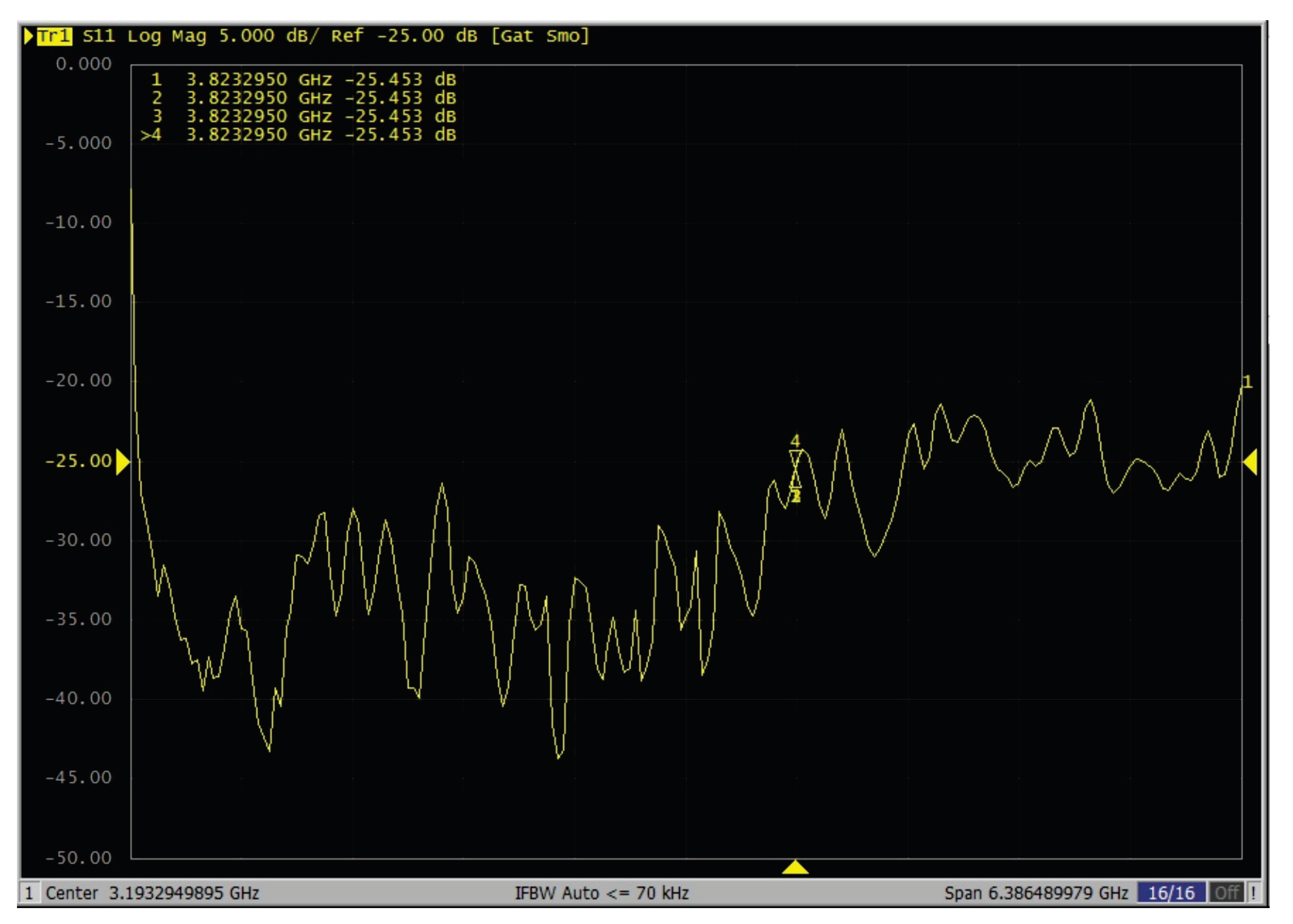
The parameter of the fabricated antenna is shown in Figure 5. The parameter is defined as the reflection coefficient between the port impedance and the network’s input impedance, and it shows how much power is reflected back at the antenna port due to mismatch from the transmission line, and it measures the amount of energy returning to the analyzer. The amount of energy that returns to the analyzer is affected directly by how well the antenna is matched to the transmission line. A small indicates a significant amount of energy has been delivered to the antenna. A good compromise is at −13 dB. If is smaller than −13 dB, the impact from reflections will not be seen on the transmitted signal. Figure 5 shows the measured parameter where parameter values are below −20 dB for frequency range between 100 kHz and 6.3 GHz.
4. System Overview and Operation
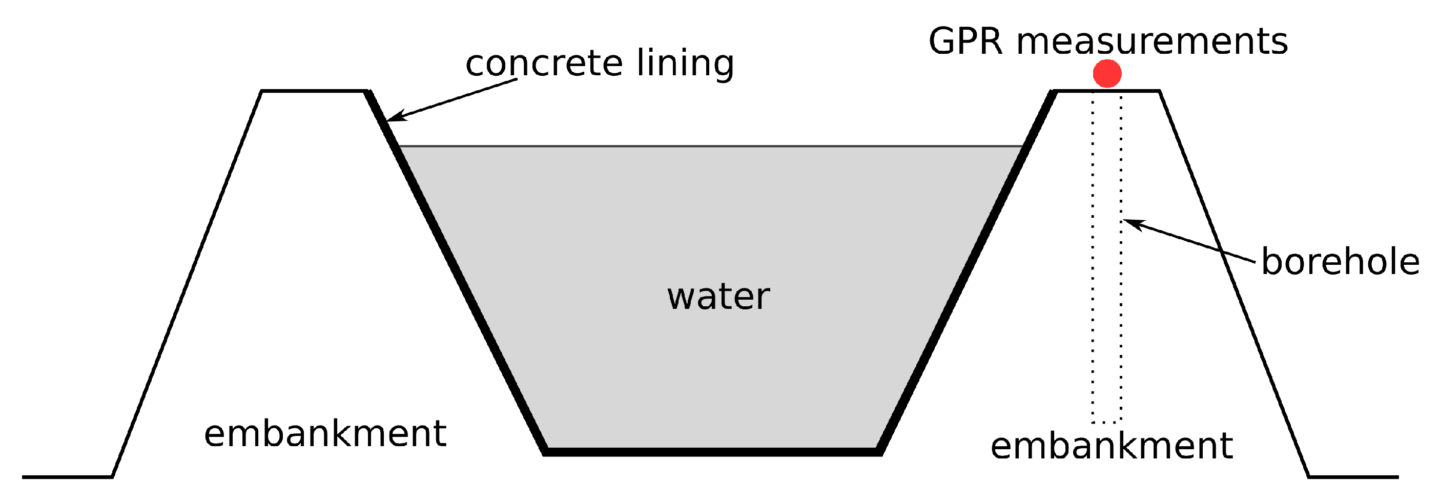
This paper aimed to detect changes in soil moisture over more considerable distances. Figure 6 shows the water canal’s cross-section. The water canal is raised over the ground surface using an embankment of compacted soil. The inside of the water canal is lined with a layer of concrete to retain water. If there is a lining leak, the embankment’s soil moisture will change. Therefore, constant soil moisture monitoring in the embankment is performed since higher water content can cause soil erosion, and less water is distributed using a water canal. This paper proposes a cross-hole GPR system for autonomous monitoring over larger sections. The proposed system could reduce maintenance costs and could raise water distribution efficiency.
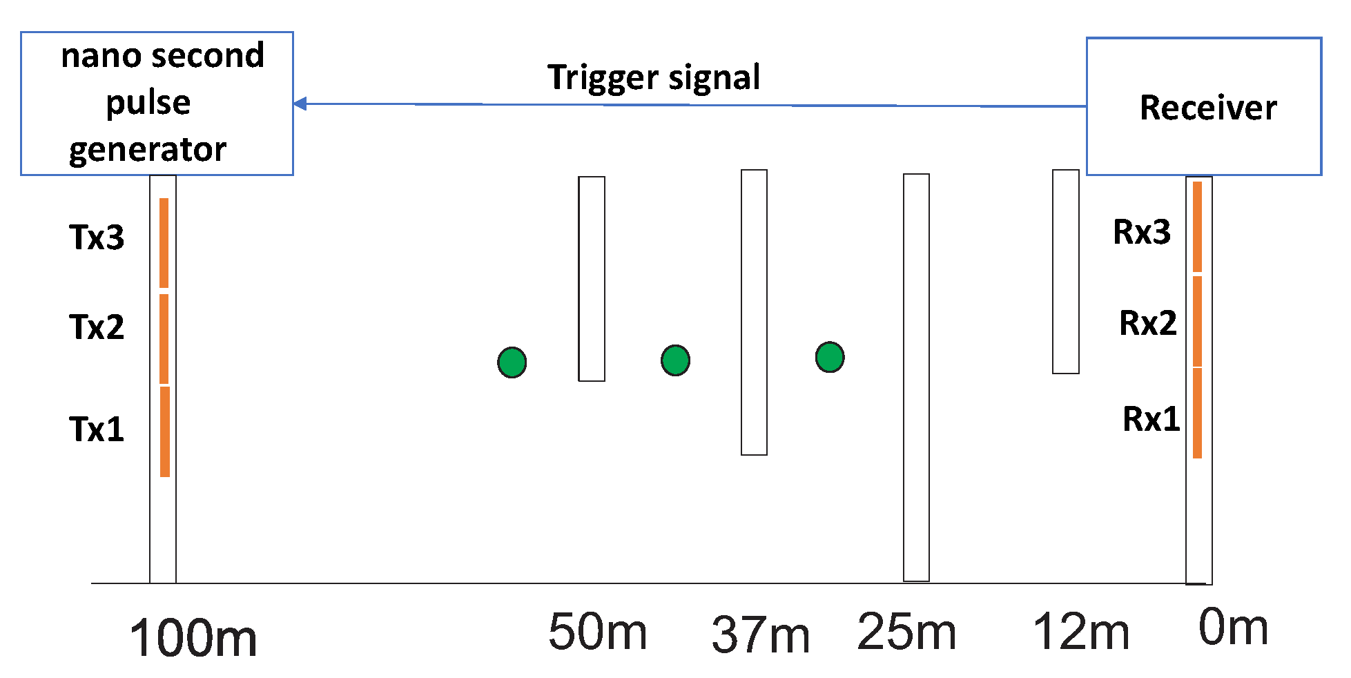
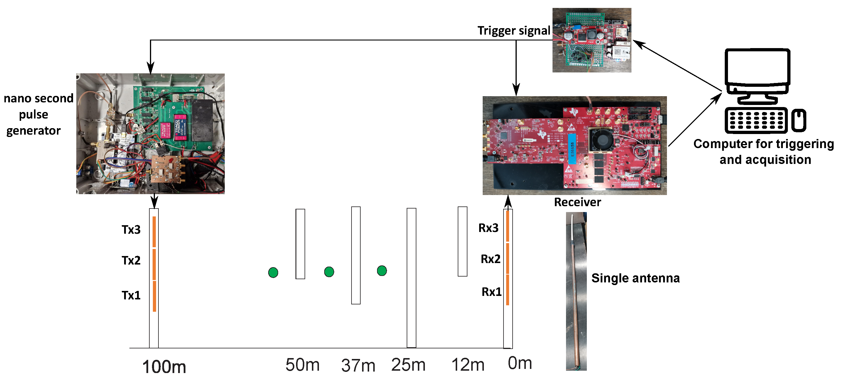
The system overview and the borehole placement at the test area are shown in Figure 7. The transmitter (Tx) and receiver (Rx) of the designed system were placed on opposite sides of the observation area. The Tx unit transmits nanosecond pulses and the Rx unit is receiving them using a high-speed data acquisition card with a sampling rate of 3 Giga Samples per second. On the Rx side the timing unit was allocated that triggers the pulse generator at the Tx side and enables data acquisition. A series of pulses were transmitted using the pulse repetition frequency (PRF) of 1 kHz. Ten received pulses were averaged at the Rx side.
The boreholes for the Tx and Rx sides were 100 m apart, and additional boreholes were drilled at distances of 12.5, 25, 37.5, and 50 m from the Rx side. A total of six antennas were placed at different depths inside the Rx and Tx boreholes, and the system switched between three Tx and three Rx antennas, obtaining all 3 × 3 combinations. The antennas were designed to be 1.55 m in length, therefore, 3 antennas were placed inside the boreholes at depths of 2, 4, and 6 m. The soil moisture was measured by the soil moisture sensor buried at the depth of 2 m at three locations: 31, 43, and 56 m from the Rx borehole.
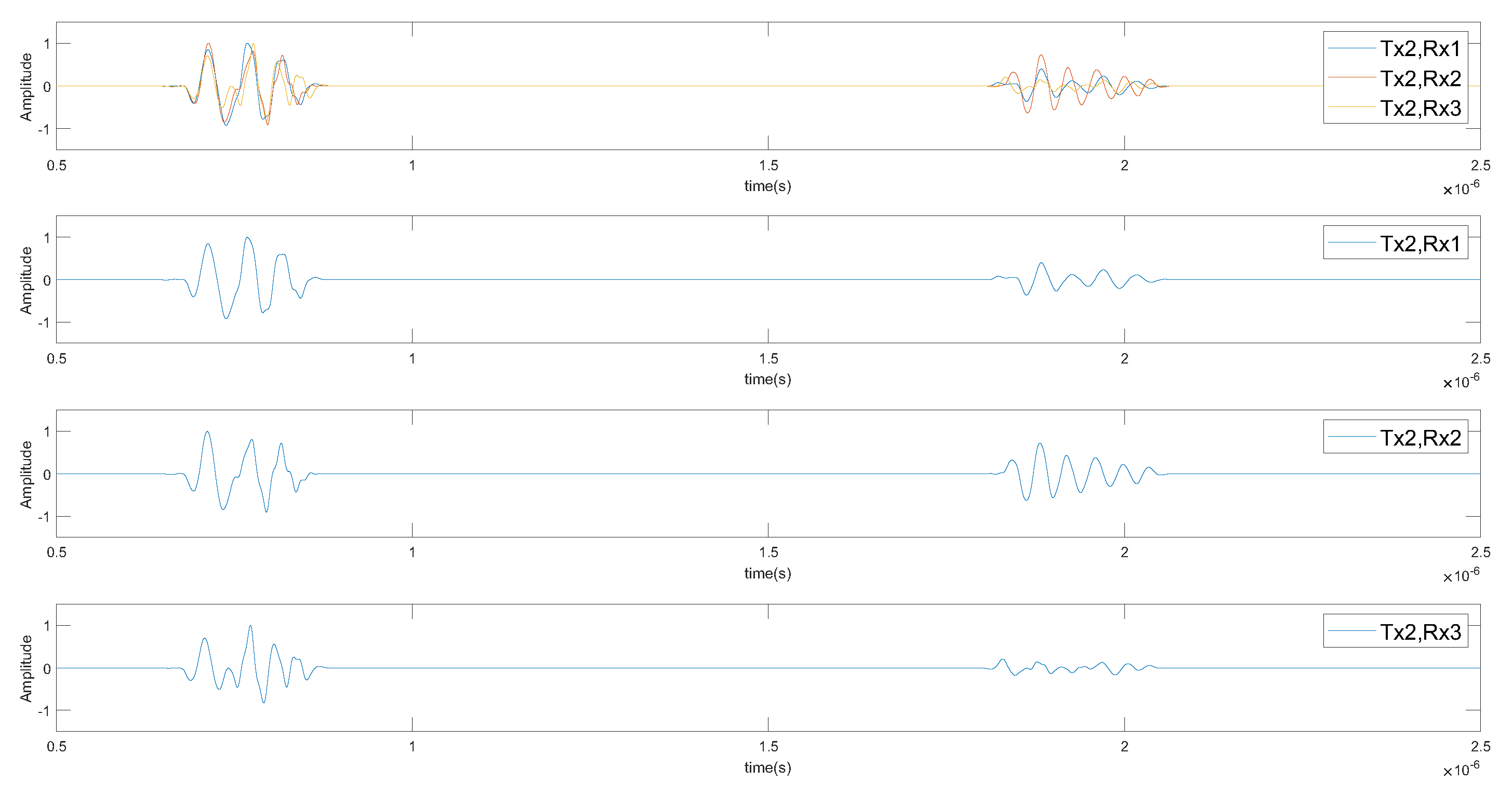
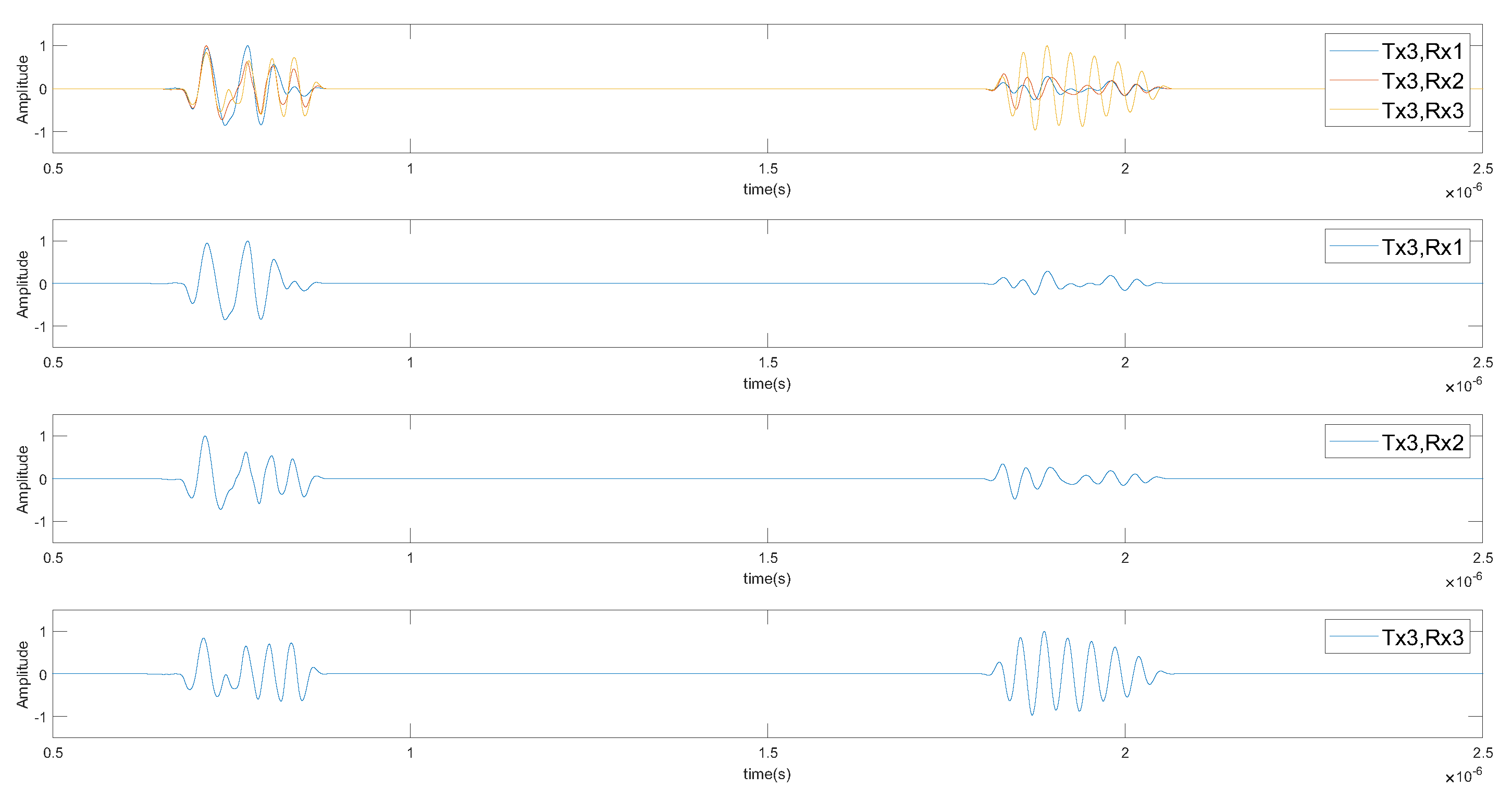
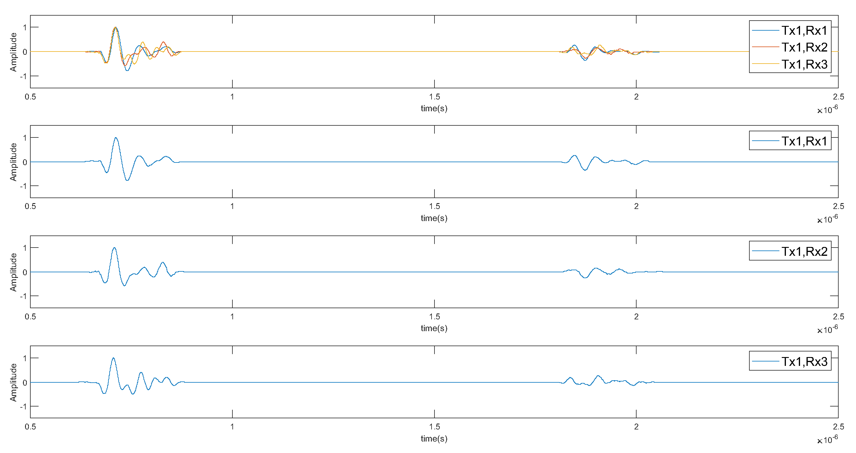
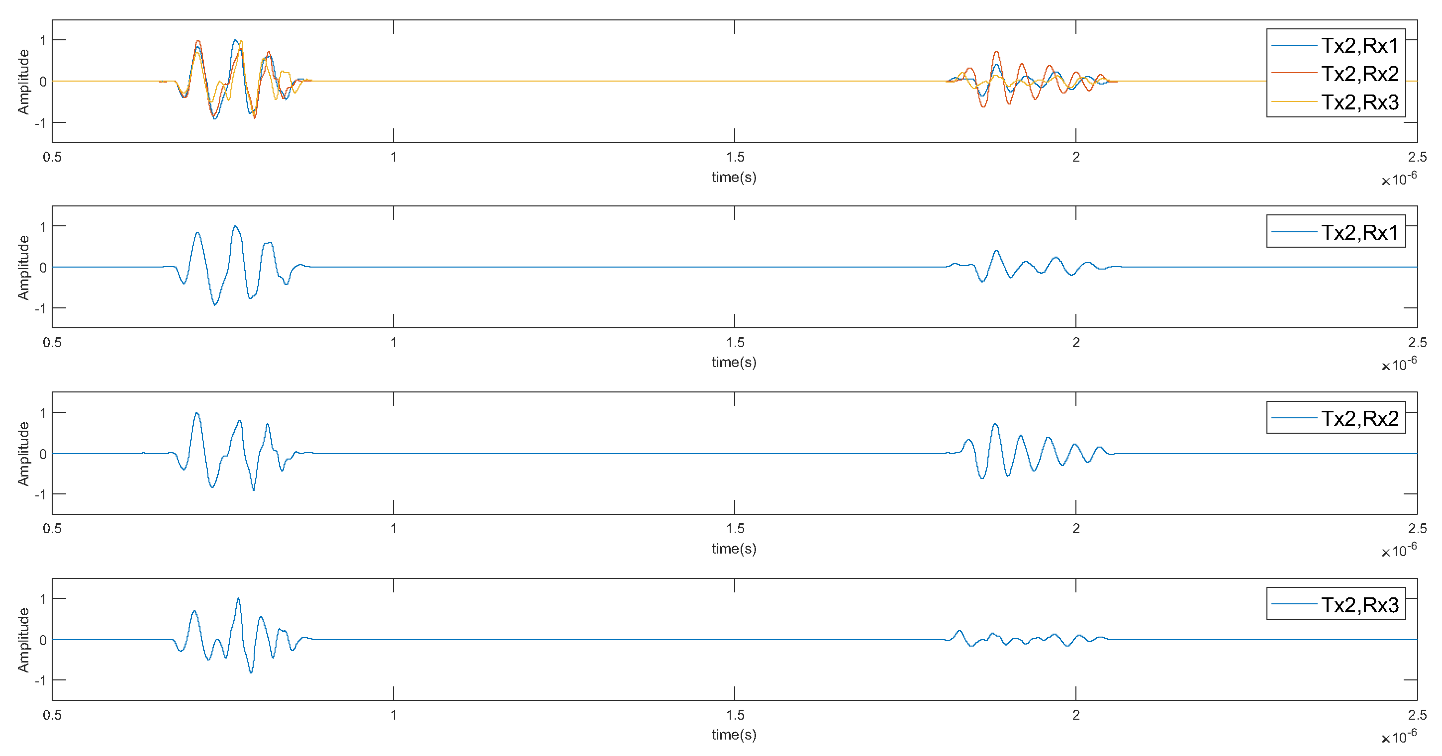
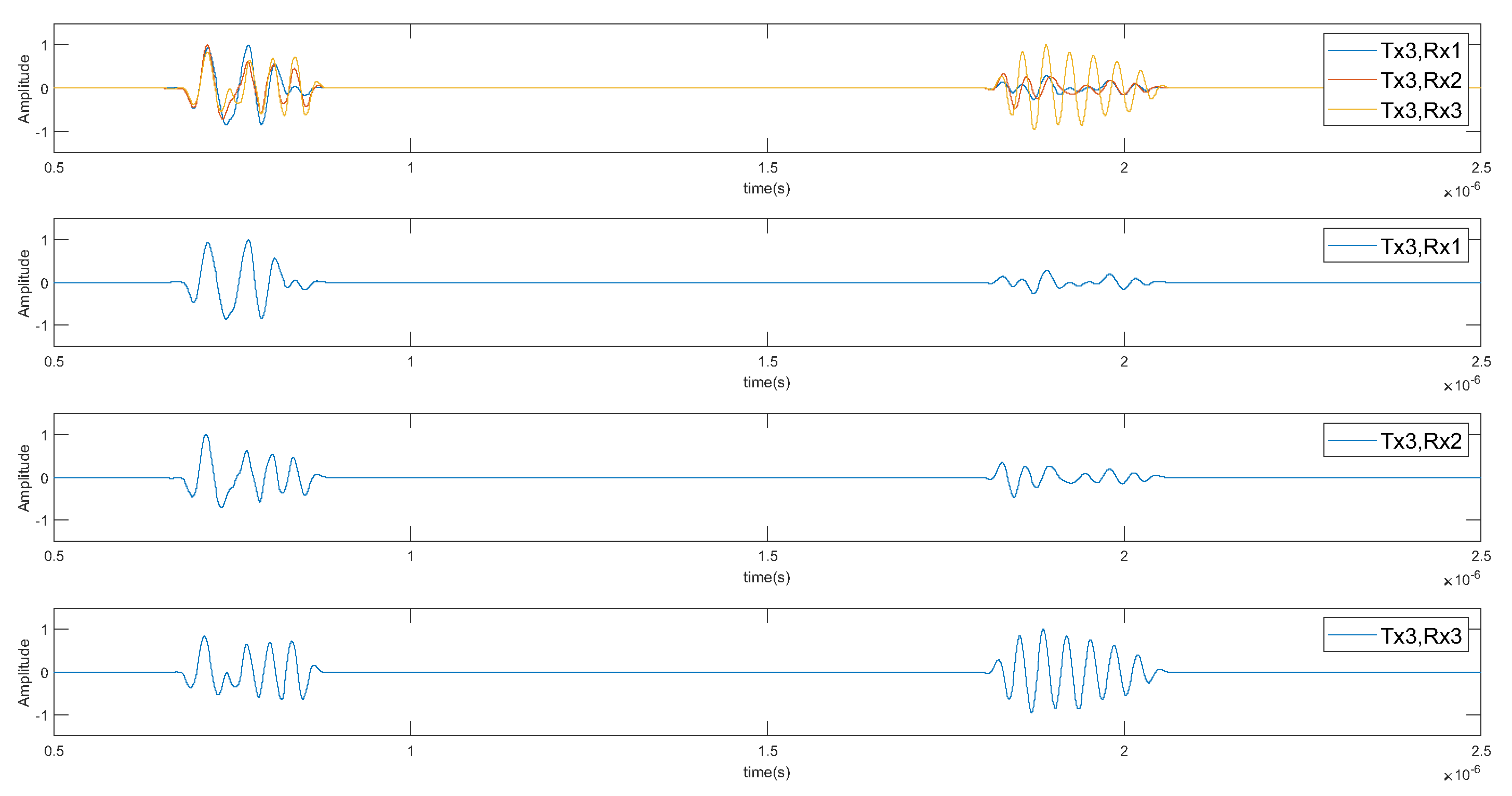
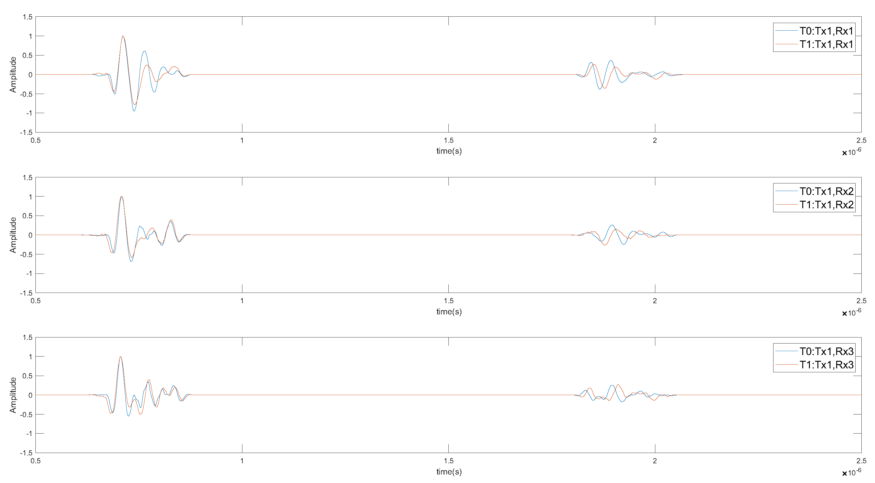
The signal’s time dependency for all three Rx antennas and all Tx antennas are shown in Figure 8, Figure 9 and Figure 10. From Figure 8, it can be seen that after the acquisition starts the transmitted signal can be detected on all the receiver’s antenna. The signal is delayed by the time trigger signal needs to travel 100 m from Rx side to Tx side over the coaxial cable (15 μs). The ground signal can be spotted at time 0.8 μs after triggering (signal propagates over the coaxial cable with a speed of , where c is the speed of EM wave in free space, resulting in 0.49 μs, and the ground signal propagates for additional 0.33 μs). It can be noticed that the designed antenna filters the input pulse from 2 ns to 57 ns at the receiver. This is due to the not optimally matched and balanced antenna resistance, which was approx. 200 Ω. The antenna was not designed and fabricated optimally. Nevertheless, the proposed system is used for soil moisture estimation and soil moisture change detection.
Figure 8, Figure 9 and Figure 10 show the signals received when Tx1–Tx3 are transmitting one-by-one and antennas Rx1–Rx3 are all receiving transmitted signals. The air-coupled signals have a constant delay. Figure 8, Figure 9 and Figure 10 show the acquisition for dry soil condition.
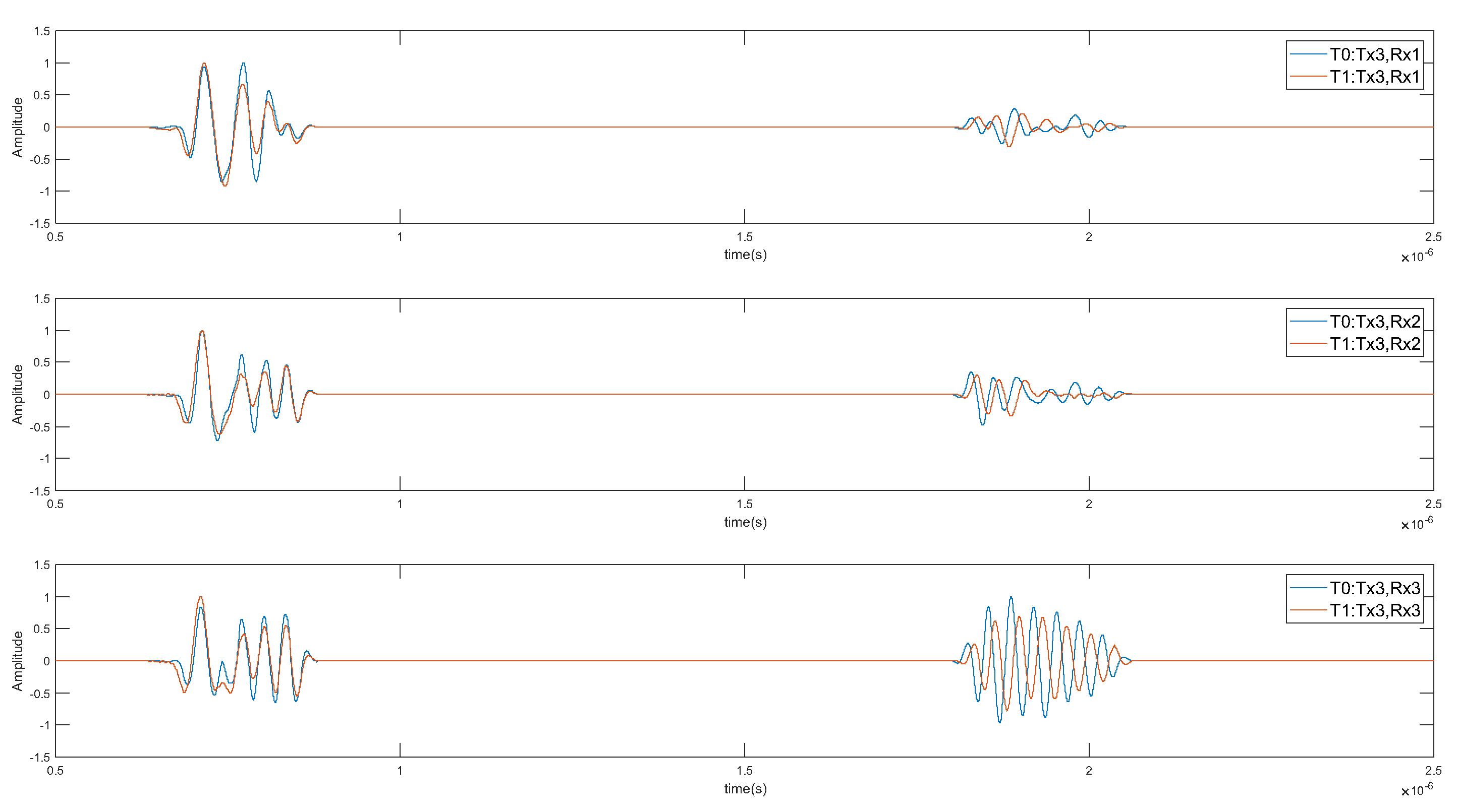
The dielectric constant was estimated using the Topp model [38] given in (2) and volumetric soil moisture was estimated with (2). Using the time delay of the received signal the dielectric constant was estimated to be 7.85 in dry conditions, resulting in 15% volumetric moisture and a propagation speed of . Several experiments were made where 800 L of water were poured into a borehole installed at 50 m from the Rx borehole within 10 min. Figure 11, Figure 12 and Figure 13 show time delayed signals before event and 1 h after the event. It is clearly visible that the received signals were additionally delayed due to the change in the soil moisture content. The measurements showed that the soil moisture in the upper layers changed from 15 to 19% of volumetric moisture.
The proposed system can cause safety concerns since the RF amplitudes are in the 1 kV range. Following the European Council recommendation on the limitation of exposure of the general public to electromagnetic fields (0 Hz to 300 GHz) 1999/519/EC, the reference levels for electric, magnetic, and electromagnetic fields should not exceed values presented in the first row of Table 1. Electromagnetic field values were estimated to ensure the proposed cross-hole GPR system complies with the 1999/519/EC recommendations, as shown in the second row of Table 1. The proposed system operates within 1999/519/EC limits for a frequency range of 10–400 MHz. Nevertheless, safety measures to protect the researchers and the environment were taken, such as limited exposure time, personal protection equipment, etc.
5. Regression Convolutional Neural Network
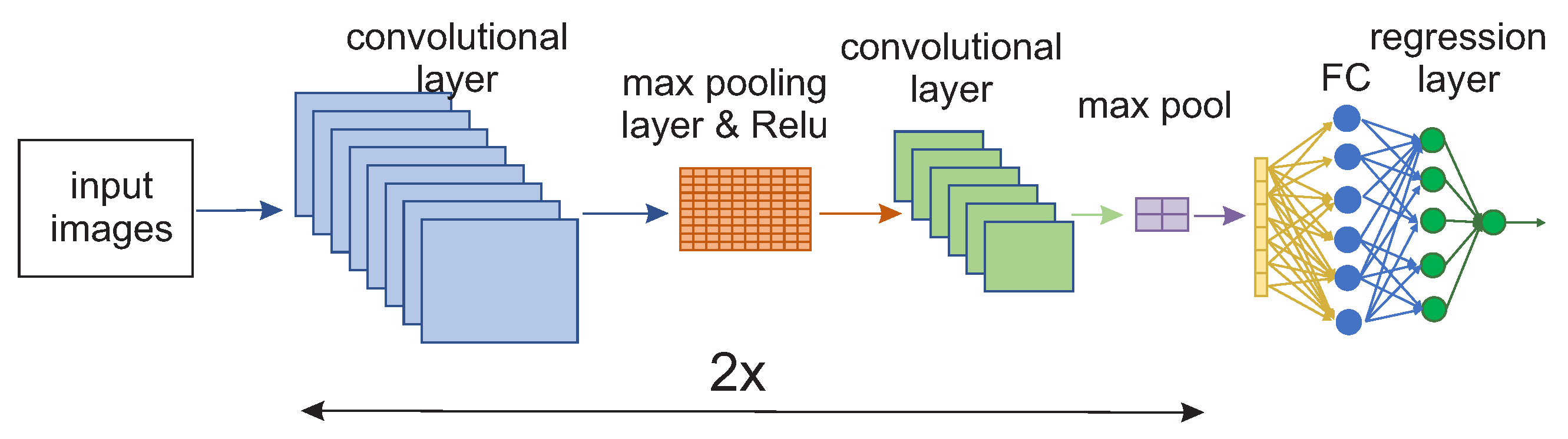
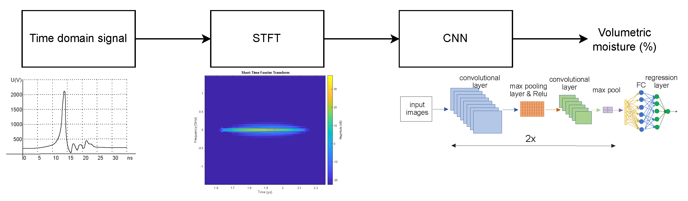
A CNN represent a series of filtering operations to extract features from the data and weight estimation, using regularization layers and closing a network with the fully connected layers. The STFT data are filtered by a series of 2D convolutional filters or kernels, and fed to a non-saturating activation function using the special rectified linear units (ReLU). The structure of proposed 2D regression CNN (2DCNN) is shown in Figure 14. The structure of convolutional layer, max-pooling, ReLU, second convolutional layer, and max-pooling is repeated two times in a series in the proposed 2DCNN, and is followed by a fully connected layer and a regression layer. The 2D convolution extracts features using the local neighborhood. The feature evaluation is based on additive bias, and the result is estimated with the sigmoid function. Features compose the feature map, a 2D image containing the values of the extracted features. The value of extracted feature at position in the j-th feature map in the i-th layer can be estimated as
where is the hyperbolic tangent function, is the bias, m represents indexes of the feature maps in the -th layer connected to the current feature map, is the value at the position of the kernel connected to the k-th feature map, and and are the dimensions of the kernel. The resolution of the feature maps is reduced by pooling over a local neighborhood on the feature maps, and provides invariance to the distortions. The trainable parameters of the CNN are the bias and the kernel weights . The supervised learning approach was used in this paper.
5.1. 3-Dimensional Convolutional Neural Networks
The idea of this paper is to extend a 2DCNN to a 3D regression CNN (3DCNN). The 2DCNN extracts 2D feature maps which represent features from the spatial dimensions only. A 3DCNN can enable both spatial and temporal feature extraction. The 3D convolution is represented by 3D convolutional filters or kernels. The feature maps in a 3D convolutional layer are interconnected over the temporal data inside the previous layer. This enables the extraction of temporal information. Equation (3) represents a value in the feature map at position for the 2DCNN, and can be expended into the value at the position on the j-th feature map in the i-th layer for the 3DCNN. The value is estimated as
where is the size of the 3D kernel along the temporal dimension, is the -th value of the kernel connected to the m -th feature map in the previous layer. One drawback of the proposed 3DCNN is that the 3D convolutional filter can extract only one type of feature from the frame cube. This is due to the filter weights being replicated across the whole cube. This can be resolved similar to the 2D convolution. A general design principle of CNNs is that the number of feature maps should be increased in late layers by generating multiple types of features from the same set of lower-level feature maps. Therefore, by applying multiple 3D convolutions with distinct filter weights to the same location in the previous layer would enable multiple feature extraction.
5.2. Pre-Processing of Acquired Data Using STFT
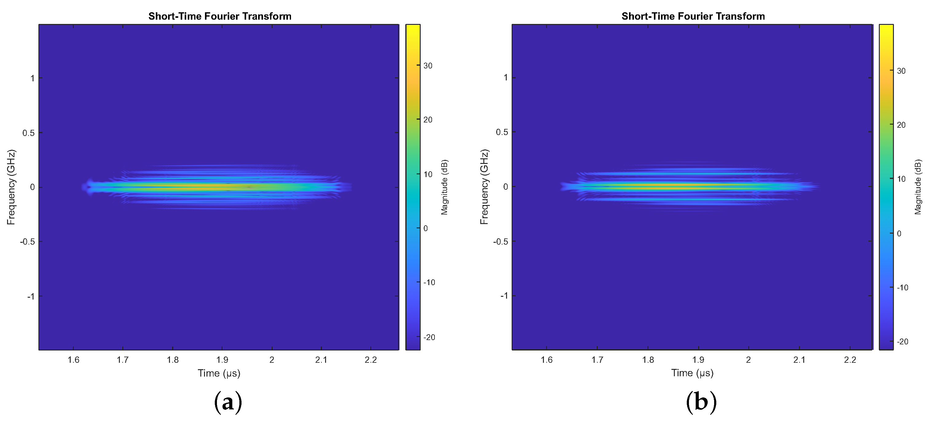
Figure 15 and Figure 16 shows measurements and comparison in dry conditions. The received signal can be divided into an air-coupled signal and a ground-coupled signal. The air-coupled signal represents the first part of the signal that propagates through the air and partly over the ground. The air component is much higher in the amplitude than the ground component. Therefore, we decided to observe just the received signal that propagates over the ground. The 1D signal was sampled using the sample frequency of 3 GHz and the acquisition lasted for 4 μs. Using a 1D signal process (i.e., data series) using CNN, the 1D signal is transformed into a 2D signal or image using STFT. The STFT of the received signal is shown in Figure 17a. The Hamming window of size 1024 samples and overlapping of 1023 samples was used to produce a 2D image 1024 × 1024 pixels in size. The STFT of the received signal on antenna Rx2 using transmitting antenna Tx2 in the dry condition and after 800 L of water were poured into borehole, is shown in Figure 17b. After the event, higher frequencies within the STFT spectrogram were much more visible.
Figure 17a,b represent spectrograms of the received signal before and after the water was poured into the borehole. The change in frequency and its phase components are clearly evident. The complex values regression CNN is used to estimate soil moisture using the designed system.
6. Data Processing Using CNN
The soil moisture can be estimated by processing the data using analysis of time delayed signals. To perform a tomography, many antennas or moving antenna platform would be needed. The system was designed to monitor the soil moisture of the canal which supplies a hydro-power station, constantly between two boreholes and detect possible leaks. To process the data, we propose to use the CNNs to extract changes in the soil moisture automatically. Changes in the soil moisture can also be caused by longer rain periods. The acquired data were correlated with the rainy days’ data, and it was found that the estimated dielectric constant depends on an antenna’s position within the borehole. The proposed system has an additional feature, since the air-coupled signal was attenuated strongly on the rainy days.
Figure 18 shows proposed data processing procedure. The radar signals are acquired with proposed cross-hole GPR system. The serialized data are then transformed into an image using STFT. To extract features from the acquired signals automatically, a CNN-based regression network was designed to process the 1D data series. In addition, a 3D regression CNN that can analyze data series and characterize the content of the soil moisture is proposed in this paper.
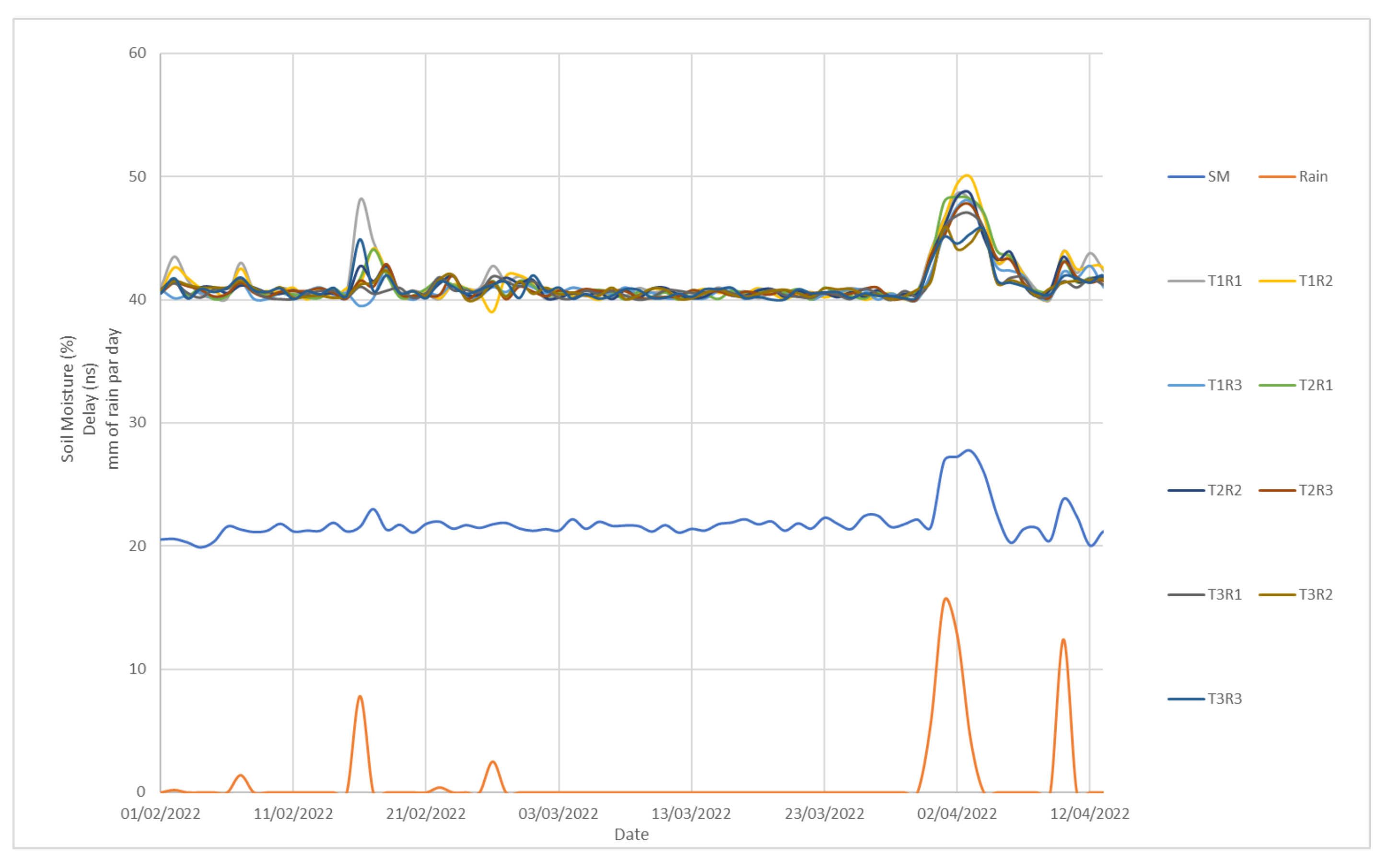
Figure 19 shows amount of rain in mm, average measurements of soil moisture using buried soil moisture sensors and delays between signals on Tx and Rx antennas in ns from 1 February till 15 April 2022. In that period, rain fell seven times and the amount of rain was between 0.5 mm to 12 mm per day. Soil moisture sensors buried below surface were capturing only 2 events on 1 April and 10 April. The delays between Tx and RX were randomly changing for all events, except the last 2. We decided to exclude data from continuous data acquisition and from training, validation, and testing when the amount of rain was below 12 mm per day.
All acquired data in the span of 73 days were used to test the proposed system and volumetric moisture. In addition, a second experiment was performed in which 800 L of water was poured in the specially prepared boreholes. Goal of the second experiment was to track changes in soil moisture in the case of a sudden injection of water. This was simulated by pouring the 800 L of water in specially prepared boreholes and measurements were taken every 15 min for next 6 h.
7. Experimental Results
The soil moisture extraction experiment is divided into several steps. The first step is data preparation, and the second step is a CNN configuration. The CNN is trained and validated in the last step. The training, validation, and testing data were acquired using a custom built database. Each data set consisted of an acquisition using 800 L of water poured into four different boreholes, located at different locations. The experiment was repeated four times, and Tx and Rx positions were swapped each time. The data were acquired every 30 min for 12 h after water injection, and the reference measurements were acquired using soil moisture sensors buried at the locations marked in Figure 20. Each batch consisted of a hundred acquisitions of each measurement. Ten batches were used for CNN training, which covered a thousand samples for each measurement. The samples are divided equally into training, validation, and testing data sets.
The acquired data were firstly transformed using the STFT. The 3D convolution was applied, with a kernel size of . The 3D max-pooling operation was applied with dimensions of , followed by the batch normalization layer. The 3D convolutional layer was applied once again with the 3D max-pooling layer and batch normalization. The flatten, dense, and activation ReLU layers were applied, followed by the dense, ReLU activation, dense, and activation layers with a sigmoid function. The model was compiled with an Adam optimizer, a learning rate of and mean square error loss function. Too many layers in the network can cause overfitting. The overfitting prevents the network from processing non-learned samples accurately. The number of filters or kernels and kernel size and stride were determined experimentally.
The training and validation data parameters are reported in Table 2. Table 2 summarizes the measured relative soil moisture SM (%), and measured time delay between the transmitted signal and the groundcoupled signal at the Rx for all measurements. More than 20,000 measurements were made using the same distance between the Tx and Rx and different combinations. The measurements were sorted regarding the measured soil moisture, as shown in the first column of Table 2. The reference soil moistures, shown in the last three columns of Table 2, were measured at three different locations, as shown in Figure 7. The reference measurements were averaged, and the average soil moisture was used as a target value in the supervised CNN learning. The reference soil moisture sensors were located 2 m below the surface, and the boreholes for water injection were 2–3 m in depth. The soil in the experiments was very dry at the beginning of the experiments, and the soil moisture was increased gradually by pouring several 1000 L of water into the boreholes to cover soil moisture between 15–45%, as shown in the first column of Table 2.
Table 3 shows a comparison of different variations of the proposed method. Different network configurations are compared. The regression network (RN) depicted in Figure 14 is compared to the method where the input data were pre-processed using STFT and trained with the RN, 3DCNN trained using the original data, 3DCNN trained using STFT pre-processed data. The results reported in Table 3 show that all the presented methods can estimate soil moisture using the regression convolutional network. It is interesting that 1D data are not appropriate for a current configuration resulting in a mean square error (MSE) of 25, 3.4, 27.7, and 1.14, which shows clearly that the RN and 3DCNN methods cannot estimate the time delay using the regression approach. By converting 1D data to the 2D data the RN and 3DCNN methods can model the time delay efficiently, and thus predict the soil moisture. The 3DCNN method provided the best results in MSE measurements, followed by the RN method.
8. Conclusions
This paper presents automated soil moisture estimation using a custom-built system for cross borehole pulse transmission and soil moisture estimation using time domain data and 3DCNN. The novelty in this paper is the soil moisture extraction form real valued data using the proposed GPR system. The efficiency of CNN-based soil moisture extraction depends on the pre-processing technique; in this case, STFT, which is proven as a suitable approach for deep learning algorithms. The STFT provided higher accuracy, being more robust on measurement uncertainty and bias. The impact on the accuracy of soil moisture recognition was observed for regression-based estimation and regression-based estimation using a 3DCNN. The simple network can extract the soil moisture parameters efficiently, and the accuracy can be increased for when 1D data series is transformed using STFT into a 2D image. The advantage of the proposed system is efficient soil moisture estimation using a 3DCNN regression network, thus providing a simple data processing technique with high accuracy.
Preliminary research presented in this paper shows the ability to detect soil moisture changes over a large area. Further research should combine several proposed systems arranged in sections over the lined water canal’s full-length (several km). A network system of proposed cross-hole GPR systems could provide automated leak detection in lined water canals over large distances.
Author Contributions
Conceptualization, M.M. and D.G.; methodology, M.M. and D.G.; software, B.P., A.S. and D.G.; validation, B.P. and D.G.; formal analysis, B.P. and D.G.; investigation, B.P., D.G. and A.S.; resources, D.G. and A.S.; data curation, M.M. and D.G.; writing—original draft preparation, B.P., M.M. and D.G.; writing—review and editing, A.S.; visualization, D.G.; supervision, A.S. and D.G.; project administration, D.G.; funding acquisition, D.G. All authors have read and agreed to the published version of the manuscript.
Funding
This research was funded by the Slovenian Research Agency (ARRS) Research program number P2-0065.
Data Availability Statement
Not applicable.
Conflicts of Interest
The authors declare no conflict of interest.
Abbreviations
The following abbreviations are used in this manuscript:
| FMCW | Frequency Modulated Continuous Wave |
| SFCW | Stepped Frequency Continuous Wave |
| ADC | Analog-to-Digital converters |
| IF | Intermediate Frequency |
| GPR | Ground Penetrating Radar |
| RF | Radio Frequency |
| IDFT | Inverse Discrete Fourier Transform |
| CNN | Convolutional Neural Networks |
| 3D | 3-Dimensional |
| 1D | 1-Dimensional |
| 2D | 2-Dimensional |
| STFT | Short Time Fourier Transform |
| MOSFET | Metal-Oxide-Semiconductor Field-Effect Transistor |
| ReLU | Rectified Linear Unit |
| 2DCNN | 2-Dimensional Convolutional Neural Networks |
| 3DCNN | 3-Dimensional Convolutional Neural Networks |
| RN | Regression Network |
| MSE | Mean Square Error |
References
- Taylor, J.D. Ultrawideband Radar: Applications and Design; CRC Press: Boca Raton, FL, USA, 2012. [Google Scholar]
- Purnomo, A.T.; Komariah, K.S.; Lin, D.B.; Hendria, W.F.; Sin, B.K.; Ahmadi, N. Non-Contact Supervision of COVID-19 Breathing Behaviour With FMCW Radar and Stacked Ensemble Learning Model in Real-Time. IEEE Trans. Biomed. Circuits Syst. 2022, 16, 664–678. [Google Scholar] [CrossRef] [PubMed]
- Hovanessian, S.A. Radar System Design and Analysis; Artech House Inc.: Norwood, MA, USA, 1984. [Google Scholar]
- Skolnik, M.I.M.I. Introduction to Impulse Radar; Naval Research Laboratory: Washington, DC, USA, 1991. [Google Scholar] [CrossRef]
- Richards, M.A.; Scheer, J.A.; Holm, W.A. Principles of Modern Radar: Basic Principles; Institution of Engineering and Technology: Raleigh, NC, USA, 2010. [Google Scholar]
- Nguyen, C.; Park, J. Stepped-Frequency Radar Sensor Analysis. In Stepped-Frequency Radar Sensors; Springer International Publishing: Cham, Switzerland, 2016; pp. 39–64. [Google Scholar] [CrossRef]
- Kong, F.N.; By, T.L. Performance of a GPR system which uses step frequency signals. J. Appl. Geophys. 1995, 33, 15–26. [Google Scholar] [CrossRef]
- Sugak, V.G.; Sugak, A.V. Phase Spectrum of Signals in Ground-Penetrating Radar Applications. IEEE Trans. Geosci. Remote. Sens. 2010, 48, 1760–1767. [Google Scholar] [CrossRef]
- Xu, Z.; Baker, C.J.; Pooni, S. Range and Doppler Cell Migration in Wideband Automotive Radar. IEEE Trans. Veh. Technol. 2019, 68, 5527–5536. [Google Scholar] [CrossRef]
- Ju, Y.; Jin, Y.; Lee, J. Design and implementation of a 24 GHz FMCW radar system for automotive applications. In Proceedings of the 2014 International Radar Conference, Lille, France, 13–17 October 2014; pp. 1–4. [Google Scholar] [CrossRef]
- Umehira, M.; Okuda, T.; Wang, X.; Takeda, S.; Kuroda, H. An Adaptive Interference Detection and Suppression Scheme Using Iterative Processing for Automotive FMCW Radars. In Proceedings of the 2020 IEEE Radar Conference (RadarConf20), Florence, Italy, 21–25 September 2020; pp. 1–5. [Google Scholar] [CrossRef]
- Sato, M.; Thierbach, R. Analysis of a borehole radar in cross-hole mode. IEEE Trans. Geosci. Remote Sens. 1991, 29, 899–904. [Google Scholar] [CrossRef]
- Farquharson, G.; Langman, A.; Inggs, M. Detection of water in an airport tarmac using SFCW ground penetrating radar. In Proceedings of the IEEE 1999 International Geoscience and Remote Sensing Symposium, IGARSS’99 (Cat. No.99CH36293), Hamburg, Germany, 28 June–2 July 1999; Volume 3, pp. 1749–1751. [Google Scholar] [CrossRef]
- Hamran, S.; Langley, K. A 5.3 GHz step-frequency GPR for glacier surface characterisation. In Proceedings of the Tenth International Conference on Grounds Penetrating Radar, GPR 2004, Delft, The Netherlands, 21–24 June 2004; pp. 761–764. [Google Scholar]
- Bende, R.; Kulkarni, A.; Khandare, A.; Bakade, K. Transceiver module of GPR for soil parameter measurement. In Proceedings of the 2017 International Conference on Wireless Communications, Signal Processing and Networking (WiSPNET), Chennai, India, 22–24 March 2017; pp. 1394–1397. [Google Scholar] [CrossRef]
- Langman, A.; Inggs, M. A 1–2 GHz SFCW radar for landmine detection. In Proceedings of the 1998 South African Symposium on Communications and Signal Processing-COMSIG ’98 (Cat. No. 98EX214), Rondebosch, South Africa, 8 September 1998; pp. 453–454. [Google Scholar] [CrossRef]
- Sipos, D.; Gleich, D. Design of Small Sized SFCW Radar for Landmine Detection. In Proceedings of the 2019 PhotonIcs Electromagnetics Research Symposium-Spring (PIERS-Spring), Rome, Italy, 17–20 June 2019; pp. 3983–3986. [Google Scholar] [CrossRef]
- Hu, Z.; Zeng, Z.; Wang, K.; Feng, W.; Zhang, J.; Lu, Q.; Kang, X. Design and Analysis of a UWB MIMO Radar System with Miniaturized Vivaldi Antenna for Through-Wall Imaging. Remote Sens. 2019, 11, 1867. [Google Scholar] [CrossRef]
- Li, Y.C.; Oh, D.; Kim, S.; Chong, J.W. Dual Channel S-Band Frequency Modulated Continuous Wave Through-Wall Radar Imaging. Sensors 2018, 18, 311. [Google Scholar] [CrossRef] [PubMed]
- Inanan, G.; Pay, G.; Hamurcu, V.; Sutcuoglu, O. Handheld Ultra-Wideband Through-Wall Radar. In Proceedings of the 2017 Seminar on Detection Systems Architectures and Technologies (DAT), Algiers, Algeria, 20–22 February 2017; pp. 1–6. [Google Scholar] [CrossRef]
- Lu, B.; Song, Q.; Zhou, Z.; Wang, H. A SFCW radar for through wall imaging and motion detection. In Proceedings of the 2011 8th European Radar Conference, Manchester, UK, 9–14 October 2011; pp. 325–328. [Google Scholar]
- Beev, N.; Keller, J.; Mehlstäubler, T.E. Note: An avalanche transistor-based nanosecond pulse generator with 25 MHz repetition rate. Rev. Sci. Instrum. 2017, 88, 126105–126115. [Google Scholar] [CrossRef] [PubMed]
- Matiss, A.; Poloczek, A.; Stohr, A.; Brockerhoff, W.; Prost, W.; Tegude, F.J. Sub-Nanosecond Pulse Generation using Resonant Tunneling Diodes for Impulse Radio. In Proceedings of the 2007 IEEE International Conference on Ultra-Wideband, Singapore, 24–26 September 2007; pp. 354–359. [Google Scholar] [CrossRef]
- Johnson, J.M. 10 kV, 44 ns pulse generator for 1 kHz trigatron reprate operation of NLTL. In Proceedings of the 2014 IEEE International Power Modulator and High Voltage Conference (IPMHVC), Santa Fe, NM, USA, 1–5 June 2014; pp. 108–110. [Google Scholar] [CrossRef]
- Han, J.; Nguyen, C. On the development of a compact sub-nanosecond tunable monocycle pulse transmitter for UWB applications. IEEE Trans. Microw. Theory Tech. 2006, 54, 285–293. [Google Scholar] [CrossRef]
- Takahashi, K.; Igel, J.; Preetz, H.; Kuroda, S. Basics and Application of Ground-Penetrating Radar as a Tool for Monitoring Irrigation Process. In Problems, Perspectives and Challenges of Agricultural Water Management; Kumar, M., Ed.; IntechOpen: Rijeka, Croatia, 2012; Chapter 8. [Google Scholar] [CrossRef]
- Karlsen, B.; Larsen, J.; Sorensen, H.; Jakobsen, K. Comparison of PCA and ICA based clutter reduction in GPR systems for anti-personal landmine detection. In Proceedings of the 11th IEEE Signal Processing Workshop on Statistical Signal Processing (Cat. No.01TH8563), Singapore, 8 August 2001; pp. 146–149. [Google Scholar] [CrossRef]
- Stone, J.V. Independent component analysis: An introduction. Trends Cogn. Sci. 2002, 6, 59–64. [Google Scholar] [CrossRef] [PubMed]
- Li, Y.; Zhao, Z.; Luo, Y.; Qiu, Z. Real-Time Pattern-Recognition of GPR Images with YOLO v3 Implemented by Tensorflow. Sensors 2002, 20, 59–64. [Google Scholar] [CrossRef] [PubMed]
- Hassaballah, M.; Awad, A. (Eds.) Deep Learning in Computer Vision: Principles and Applications, 1st ed.; CRC Press: Boca Raton, FL, USA, 2020. [Google Scholar] [CrossRef]
- Zayed, M.E.; Zhao, J.; Li, W.; Sadek, S.; Elsheikh, A.H. Chapter three—Applications of artificial neural networks in concentrating solar power systems. In Artificial Neural Networks for Renewable Energy Systems and Real-World Applications; Elsheikh, A.H., Abd Elaziz, M.E., Eds.; Academic Press: Cambridge, MA, USA, 2022; pp. 45–67. [Google Scholar] [CrossRef]
- Pirc, E.; Miklavčič, D.; Reberšek, M. Nanosecond Pulse Electroporator With Silicon Carbide <sc>mosfet</sc>s: Development and Evaluation. IEEE Trans. Biomed. Eng. 2019, 66, 3526–3533. [Google Scholar] [CrossRef] [PubMed]
- Sanders, J.M.; Kuthi, A.; Wu, Y.H.; Vernier, P.T.; Gundersen, M.A. A linear, single-stage, nanosecond pulse generator for delivering intense electric fields to biological loads. IEEE Trans. Dielectr. Electr. Insul. 2009, 16, 1048–1054. [Google Scholar] [CrossRef]
- Leone, M. Advances in fiber optic sensors for soil moisture monitoring: A review. Results Opt. 2022, 7, 100213. [Google Scholar] [CrossRef]
- Shlager, K.L.; Smith, G.S.; Maloney, J.G. TEM horn antenna for pulse radiation: An optimized design. IEEE 2008, 2, 201–211. [Google Scholar]
- Sagnard, F.; Fauchard, C. FDTD Modeling of a Resistively Loaded Monopole for Narrow Borehole Ground Penetrating Radar. Prog. Electromagn. Res. M 2008, 2, 201–211. [Google Scholar] [CrossRef]
- Wu, T.; King, R. The cylindrical antenna with nonreflecting resistive loading. IEEE Trans. Antennas Propag. 1965, 13, 369–373. [Google Scholar] [CrossRef]
- Topp, G.C.; Davis, J.L.; Annan, A.P. Electromagnetic determination of soil water content: Measurements in coaxial transmission lines. Water Resour. Res. 1980, 16, 574–582. [Google Scholar] [CrossRef]
Figure 1.
Schematics of the proposed pulse generator’s basic principle [32].
Figure 1.
Schematics of the proposed pulse generator’s basic principle [32].

Figure 2.
Schematic of a custom built pulse generator using four MOSFET transistors in a parallel configuration [32].
Figure 2.
Schematic of a custom built pulse generator using four MOSFET transistors in a parallel configuration [32].

Figure 3.
Nanosecond pulse generated with the proposed custom built pulse generator circuit.

Figure 4.
Designed borehole antenna used for pulse transmission [36].
Figure 4.
Designed borehole antenna used for pulse transmission [36].

Figure 5.
Measured parameter of the antenna shown in Figure 4.
Figure 5.
Measured parameter of the antenna shown in Figure 4.

Figure 6.
Cross-section of the lined water canal. GPR measurements were performed on embankment made of compacted soil.
Figure 6.
Cross-section of the lined water canal. GPR measurements were performed on embankment made of compacted soil.

Figure 7.
A system overview. Six bore-holes placed on a distance between 0 and 100 m. The acquisition system was installed into two boreholes. The green dots represent the measured soil moisture at a depth of 2 m.
Figure 7.
A system overview. Six bore-holes placed on a distance between 0 and 100 m. The acquisition system was installed into two boreholes. The green dots represent the measured soil moisture at a depth of 2 m.

Figure 8.
Signals acquired in dry conditions when Tx1 is transmitting pulses and Rx1 –3 are receiving signals.
Figure 8.
Signals acquired in dry conditions when Tx1 is transmitting pulses and Rx1 –3 are receiving signals.

Figure 9.
Signals acquired in dry conditions when Tx2 is transmitting pulses and Rx1 –3 are receiving signals.
Figure 9.
Signals acquired in dry conditions when Tx2 is transmitting pulses and Rx1 –3 are receiving signals.

Figure 10.
Signals acquired in dry conditions when Tx3 is transmitting pulses and Rx1 –3 are receiving signals.
Figure 10.
Signals acquired in dry conditions when Tx3 is transmitting pulses and Rx1 –3 are receiving signals.

Figure 11.
Signals acquired 1 h after pouring water in specially prepared boreholes. Tx1 is transmitting pulses and Rx1 –3 are receiving signals.
Figure 11.
Signals acquired 1 h after pouring water in specially prepared boreholes. Tx1 is transmitting pulses and Rx1 –3 are receiving signals.

Figure 12.
Signals acquired 1 h after pouring water in specially prepared boreholes. Tx2 is transmitting pulses and Rx1 –3 are receiving signals.
Figure 12.
Signals acquired 1 h after pouring water in specially prepared boreholes. Tx2 is transmitting pulses and Rx1 –3 are receiving signals.

Figure 13.
Signals acquired 1 h after pouring water in specially prepared boreholes. Tx3 is transmitting pulses and Rx1 –3 are receiving signals.
Figure 13.
Signals acquired 1 h after pouring water in specially prepared boreholes. Tx3 is transmitting pulses and Rx1 –3 are receiving signals.

Figure 14.
Regression-based convolutional neural network.

Figure 15.
Comparison of signals in dry condition, event T0 and 1 h after 800 L of water were injected into borehole at 50 m (event T1). The signals were acquired when Tx1 was transmitting pulses and Rx1-3 were receiving signals.
Figure 15.
Comparison of signals in dry condition, event T0 and 1 h after 800 L of water were injected into borehole at 50 m (event T1). The signals were acquired when Tx1 was transmitting pulses and Rx1-3 were receiving signals.

Figure 16.
Comparison of signals in dry condition, event T0 and 1 h after 800 L of water were injected into borehole at 50 m (event T1). The signals were acquired when Tx3 was transmitting pulses and Rx1-3 were receiving signals.
Figure 16.
Comparison of signals in dry condition, event T0 and 1 h after 800 L of water were injected into borehole at 50 m (event T1). The signals were acquired when Tx3 was transmitting pulses and Rx1-3 were receiving signals.

Figure 17.
The short -time Fourier transform of signal Tx2-Rx2, shown in Figure 9: (a) before the water was poured into borehole, and (b) after the water was poured into borehole.
Figure 17.
The short -time Fourier transform of signal Tx2-Rx2, shown in Figure 9: (a) before the water was poured into borehole, and (b) after the water was poured into borehole.

Figure 18.
Block diagram of proposed data processing procedure. Time domain signals are acquired and using an STFT transformed into an image. The image is then processed using the proposed CNN structures and the result is presented in volumetric moisture content (%).
Figure 18.
Block diagram of proposed data processing procedure. Time domain signals are acquired and using an STFT transformed into an image. The image is then processed using the proposed CNN structures and the result is presented in volumetric moisture content (%).

Figure 19.
Graph of fallen rain in mm, average measurements of soil moisture (SM in %) and delays between signals on Tx and Rx antennas in ns from 1 February until 15 April 2022.
Figure 19.
Graph of fallen rain in mm, average measurements of soil moisture (SM in %) and delays between signals on Tx and Rx antennas in ns from 1 February until 15 April 2022.

Figure 20.
A system overview with implemented nano-second pulse generator, trigger signal generator, and acquisition system.
Figure 20.
A system overview with implemented nano-second pulse generator, trigger signal generator, and acquisition system.


Table 1.
Comparison between reference levels for electric, magnetic, and electromagnetic fields and estimated levels of electric, magnetic, and electromagnetic fields emitted from proposed system in frequency range 10–400 MHz.
Table 1.
Comparison between reference levels for electric, magnetic, and electromagnetic fields and estimated levels of electric, magnetic, and electromagnetic fields emitted from proposed system in frequency range 10–400 MHz.
| Level | E-Field (V/m) | H-Field (A/m) | B-Field (μT) | Power Density (W/m2) |
|---|---|---|---|---|
| Reference | 28 | 0.073 | 0.092 | 2 |
| Estimated | 2.46 | 0.006535 | 8.227 | 0.016 |
Table 2.
Estimated soil moisture based on measured time delay. Estimated soil moisture can be compared to the referenced soil moisture, which was acquired using reference soil moisture sensors.
Table 2.
Estimated soil moisture based on measured time delay. Estimated soil moisture can be compared to the referenced soil moisture, which was acquired using reference soil moisture sensors.
| Reference Soil Moisture (int %) | Measured Time Delay (in ns) | Estimated Soil Moisture (in %) | ||
|---|---|---|---|---|
| 15 | 0 | 14 | 16 | 13 |
| 20 | 6 | 19 | 19 | 20 |
| 25 | 13 | 24 | 22 | 24 |
| 30 | 21 | 29 | 28 | 31 |
| 35 | 26 | 33 | 33 | 36 |
| 40 | 32 | 41 | 42 | 39 |
| 45 | 39 | 44 | 40 | 43 |
Table 3.
Average reference soil moisture acquired by soil moisture sensors compared to the estimated soil moisture by RN, RN + STFT, 3DCNN, and 3DCNN + STFT methods and radar data.
Table 3.
Average reference soil moisture acquired by soil moisture sensors compared to the estimated soil moisture by RN, RN + STFT, 3DCNN, and 3DCNN + STFT methods and radar data.
| Reference Soil Moisture (%) | RN | RN + STFT | 3DCNN | 3DCNN + STFT |
|---|---|---|---|---|
| 15 | 14 | 16 | 14 | 13 |
| 20 | 21 | 19 | 19 | 20 |
| 25 | 24 | 24 | 23 | 24 |
| 30 | 29 | 31 | 37 | 31 |
| 35 | 30 | 33 | 28 | 36 |
| 40 | 35 | 44 | 33 | 39 |
| 45 | 34 | 45 | 36 | 45 |
| MSE | 25 | 3.4 | 27.7 | 1.14 |
Disclaimer/Publisher’s Note: The statements, opinions and data contained in all publications are solely those of the individual author(s) and contributor(s) and not of MDPI and/or the editor(s). MDPI and/or the editor(s) disclaim responsibility for any injury to people or property resulting from any ideas, methods, instructions or products referred to in the content. |
© 2023 by the authors. Licensee MDPI, Basel, Switzerland. This article is an open access article distributed under the terms and conditions of the Creative Commons Attribution (CC BY) license (https://creativecommons.org/licenses/by/4.0/).
Share and Cite
MDPI and ACS Style
Pongrac, B.; Gleich, D.; Malajner, M.; Sarjaš, A. Cross-Hole GPR for Soil Moisture Estimation Using Deep Learning. Remote Sens. 2023, 15, 2397. https://doi.org/10.3390/rs15092397
AMA Style
Pongrac B, Gleich D, Malajner M, Sarjaš A. Cross-Hole GPR for Soil Moisture Estimation Using Deep Learning. Remote Sensing. 2023; 15(9):2397. https://doi.org/10.3390/rs15092397
Chicago/Turabian StylePongrac, Blaž, Dušan Gleich, Marko Malajner, and Andrej Sarjaš. 2023. "Cross-Hole GPR for Soil Moisture Estimation Using Deep Learning" Remote Sensing 15, no. 9: 2397. https://doi.org/10.3390/rs15092397
Note that from the first issue of 2016, this journal uses article numbers instead of page numbers. See further details here.