Neural Network Based Control of Four-Bar Mechanism with Variable Input Velocity

Abstract

For control applications, the angular velocity of the drive crank of a four-bar mechanism is traditionally assumed to be constant. In this paper, we propose control of variable velocity of the drive crank to obtain the desired output motions for the coupler point. To estimate the reference trajectory for the crank velocity, a neural network is trained with data from the kinematic model. The control law is designed from feedback linearization of the tracking error dynamics and a Proportional–Integral–Derivative (PID) controller. The applicability of the proposed scheme is validated through simulations for three variable speed profiles, obtaining excellent results from the system.

1. Introduction

When an electric motor is coupled in a four-bar mechanism, a periodically time varying torque, produced by the changing inertia of the mechanism during its rotation, is applied as an external load to the motor [1]. Different control techniques have been studied to regulate the crank angular velocity fluctuations introduced by the inertia of the rotor and the rotating bars in four-bar linkages. Among applied controllers that address this issue, are proportional–integral–derivative (PID) [1], proportional–derivative (PD) [2,3,4], nonlinear PD [5], model reference adaptive control [6], fuzzy [7], type-2 fuzzy sliding mode [8], adaptive fuzzy sliding mode [9], robust fuzzy [10], PID Fuzzy [11], PID neural network [12], PD and neural adaptive [13], moving sliding mode [14], robust backstepping control [15], and fuzzy logic controller combined with grey system modeling approach [16]. In [17], several control schemes are investigated (filtered proportional–integral–derivative, filtered sliding mode, filtered fuzzy, and filtered genetic-based reinforcement neuro-controller). In reference [18], experimental data were used to develop parametric models for a four-bar mechanism driven by a geared DC motor by employing artificial neural networks. In reference [19], PID linear control was used to control a micro-aerial-vehicle that has four flapping wings (four-bar mechanisms). In [20], the gains of a PID controller for the four-bar mechanism are optimized via evolutionary algorithms. Recently, in [21], an indirect adaptive control based on online multi-objective optimization for the velocity regulation of the four-bar mechanism was proposed. Other advanced control schemes for trajectory tracking in mechanical systems consider sliding modes [22] and Linear Matrix Inequalities (LMI) approaches [23], which are both applied for docking mechanisms. Furthermore, optimal sliding mode control has been applied in quick-return mechanisms [24]. On the other hand, fuzzy-based controlled schemes for trajectory tracking have been recently developed with applications on mobile robots with promising results [25,26,27]. In reference [25], the design of a highly efficient path-following scheme for wheeled mobile robots is proposed. Here the authors present a new controller constructed by the type-3 (T3) fuzzy logic systems (FLS) and a predictive compensator where the stability of the complete system is validated with the Lyapunov methodology. Furthermore, this scheme is tested with good performance in a chaotic generated path.

The main topic of this work is to integrate computational intelligence methods to solve the inverse kinematics problem to control a four-bar mechanism for trajectory tracking in the coupler point; this trajectory requires a variable angular velocity of the drive crank. This control scheme is defined as variable input velocity control. There are few reports of simulation studies on cases of trajectory tracking where the problem of variable input velocity control is addressed [2,3,6,15,28,29,30]. In [6], a model reference adaptive controller for the velocity regulation of a four-bar mechanism is designed. In reference [2], motion control of four-bar mechanism driven by a brushless servo motor is applied where simulation and experimental results were validated for different crank motion profiles. In [3], a PD control algorithm is employed for trajectory tracking in a four-bar mechanism which is redesigned by applying a new mass-distribution scheme. In reference [28], an integrated approach for variable input velocity servo four-bar linkages is designed in order to satisfy the kinematic requirements, reduce the shaking force and moment, improve the velocity trajectory tracking performance, and minimize the motor power dissipation where dimensions of the links, counterweights, input-velocity trajectory and controller parameters are considered as design variables simultaneously. In [15], a robust backstepping controller is designed and tested in simulation for a four-bar linkage mechanism that is driven by a DC motor, without a priori knowledge of the model parameters where five cases were examined. In reference [29,30], the problem of trajectory tracking by controlling the angular velocity of the input link is investigated in a four-bar mechanism to fulfill moving the coupler point with a constant velocity. A vision controller for regulation of the velocity of the coupler point in a four-bar mechanism was implemented in [30], where the desired trajectory for the coupler point of the mechanism is achieved by controlling the angular velocity of the crank using a feedback linearization algorithm for the error dynamics and a PID controller.

For a four-bar mechanism, the characteristics of the output movement depend on the crank’s input movement. Then, it is necessary that the designed control fulfills the mechanism desired input velocity profile in order for the output motion to follow the desired trajectory. In this work, the problem of trajectory tracking is considered; the variable input velocity control is designed to ensure that the coupler point follows a constant velocity reference. To obtain the reference for the crank velocity and to reduce the computational burden for the synthesized control, a neural network is implemented. Neural networks have been widely applied to aid the control design process for mechanisms due to their simple design and easy implementation. In [12], a feed-forward neural network is applied to predict the reference model used by a PID controller for the constant velocity of the crank.

The structure of this work is presented as follows: Section 2 explains the kinematic model for the four-bar mechanism, the DC motor and mechanical coupling mathematical models are developed, and the overall dynamic model is presented. In Section 3, the Artificial Neural Network and PID control scheme are synthesized. Section 4 presents the path for the coupler point in the mechanism, and simulation results for several cases of trajectory tracking are discussed. In Section 5, the conclusions are summarized.

2. Mathematical Model for a Motor-Driven Four-Bar Mechanism System

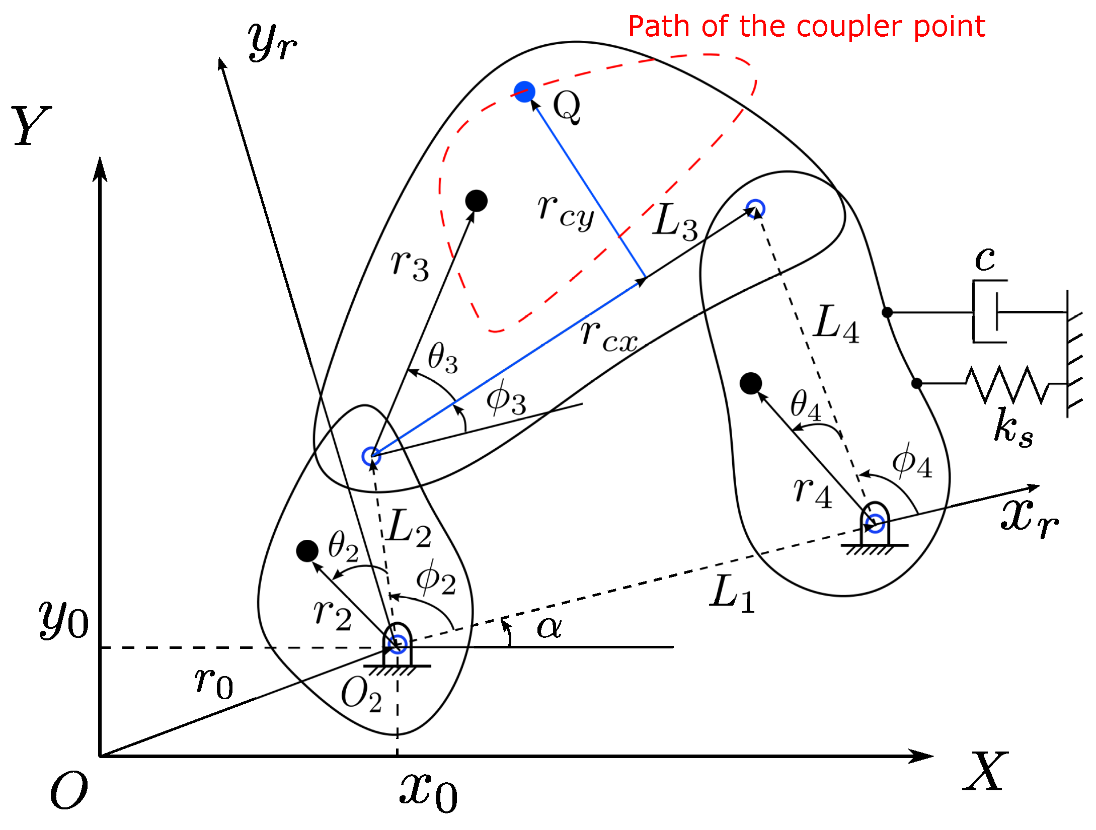
2.1. Dynamics of the Four-Bar Linkages

A general four-bar linkage is presented in Figure 1, where link $L_2$ (crank) is driven by an electrical motor, and it is able to perform a complete rotation. The link $L_3$ (coupler) performs a general motion in the plane, and it transmits the movement to link $L_4$ (rocker), which executes an oscillatory motion, and the link $L_1$ (ground) is fixed with respect to the reference frame. The kinematic model of the four-bar mechanism is defined with respect to the global reference system $\{X-Y\}$. The local reference system $\{x_r-y_r\}$ is assigned with the origin coinciding on the pivot $O_2$ of the mechanism and is specified the direction $x_r$ along of the link $L_1$. Thus, the relation between the local reference system with respect to the global $\{X-Y\}$, is defined by the translation $r_0$ and orientation $\alpha$.

The parameters in Figure 1 required to develop the dynamical model of the mechanism are summarized in

Table 1. Parameters of four-bar mechanism.

Parameter	Description for Each Link
$L_i$	length of the link i
${\varphi }_i$	angular position for link i with respect to the axis $x_r$
$m_i$	mass of link i
$J_i$	mass moment of inertia
$r_i$ and ${\theta }_i$	location of the center of mass for each link i
$r_{cx}$ and $r_{cy}$	location of point Q on link 3

. Each link has a mass of $m_i$, a mass moment of inertia with respect to the centroid $J_i$, and $L_i$ is the length of the link i. The angular positions of each link with respect to the $x_r$ axis of the base frame are denoted by ${\varphi }_2$, ${\varphi }_3$, and ${\varphi }_4$. The position vector of the center of mass for each link i is displayed by a dark circle and their locations are described by $r_i$ and ${\theta }_i$. A torsional spring with a stiffness constant $k_s$ and a torsional damper with a damping constant c are attached to the rocker link to represent a general loading situation.

Applying the Euler–Lagrange modeling methodology [1,31], the equation of motion for the mechanism, by using the crank angle ${\varphi }_2$ as the generalized coordinate, is given by

$$\frac{d}{dt}\left(\frac{\partial K}{\partial {\dot{\varphi }}_2}\right)-\frac{\partial K}{\partial {\varphi }_2}+\frac{\partial P}{\partial {\varphi }_2}+\frac{\partial D}{\partial {\dot{\varphi }}_2}=T$$

(1)

where $K,P,$ and D denote the kinetic, potential, and dissipative energies, respectively, and T is the applied external torque. The dissipation term can be neglected in the mechanism, since the damping is relatively small.

The kinetic energy of the mechanism is defined as

$${\displaystyle K=\sum _{i=2}^4\left[\frac{1}{2}{m}_i(V_{ix}^2+V_{iy}^2)+\frac{1}{2}{J}_i{\dot{\varphi }}_i^2\right]}$$

(2)

where $V_{ix}$ and $V_{iy}$ represent the components of velocity at the mass center in X and Y of the link i, and ${\dot{\varphi }}_i$ is the angular velocity of the link i.

According to the scheme in Figure 1, the kinetic energy can be expressed as

$$K=\frac{1}{2}A\left({\varphi }_2\right){\dot{\varphi }}_2^2$$

(3)

where $A\left({\varphi }_2\right)$ is defined as,

$$A\left({\varphi }_2\right)=C_0+C_1{\gamma }_3^2+C_2{\gamma }_4^2+C_3{\gamma }_{3}cos({\varphi }_2-{\varphi }_3-{\theta }_3)$$

(4)

and

$$\begin{array}{cc}\hfill C_0& =J_2+m_2{r}_2^2+m_3{L}_2^2\hfill \\ \hfill C_1& =J_3+m_3{r}_3^2\hfill \\ \hfill C_2& =J_4+m_4{r}_4^2\hfill \\ \hfill C_3& =2L_2{r}_3{m}_3\hfill \end{array}$$

From the four-bar linkage kinematics analysis position, the functions for the angular position of the coupler link, ${\varphi }_3$, and the oscillator link, ${\varphi }_4$, are determined.

The angle ${\varphi }_3$, corresponding to the orientation for coupler link, $L_3$, is defined from

$${\varphi }_3\left({\varphi }_2\right)=2arctan\left(\frac{-k_b\pm \sqrt{k_b^2-4k_a{k}_c}}{2k_a}\right)$$

(5)

where

$$\begin{array}{cc}\hfill k_a& =-l_1+(l_2+1)cos{\varphi }_2+l_3,\hfill \\ \hfill k_b& =-2sin{\varphi }_2,\hfill \\ \hfill k_c& =l_1+(l_2-1)cos{\varphi }_2+l_3,\hfill \end{array}$$

and the constants $l_1$, $l_2$, and $l_3$ are

$$\begin{array}{cc}\hfill l_1& =\frac{L_1}{L_2}\hfill \\ \hfill l_2& =\frac{L_1}{L_3}\hfill \\ \hfill l_3& =\frac{L_4^2-L_1^2-L_2^2-L_3^2}{2L_2{L}_3}\hfill \end{array}$$

The angle ${\varphi }_4$, corresponding to the orientation for oscillator link $L_4$, is defined from

$${\varphi }_4\left({\varphi }_2\right)=2arctan\left(\frac{-k_b\pm \sqrt{k_b^2-4k_d{k}_e}}{2k_d}\right)$$

(6)

where the coefficients $k_d$ and $k_e$ are

$$\begin{array}{cc}\hfill k_d& =-l_1+(1-l_4)cos{\varphi }_2+l_5,\hfill \\ \hfill k_e& =l_1-(l_4+1)cos{\varphi }_2+l_5,\hfill \end{array}$$

and the constants $l_4$ and $l_5$ are

$$\begin{array}{cc}\hfill l_4& =\frac{L_1}{L_4}\hfill \\ \hfill l_5& =\frac{L_2^2-L_3^2+L_4^2+L_1^2}{2L_2{L}_4}.\hfill \end{array}$$

From four-bar linkage kinematics analysis, the functions for the angular velocity of the coupler link, $\dot{{\varphi }_3}$ can be expressed as

$$\dot{{\varphi }_3}={\gamma }_3\dot{{\varphi }_2}$$

(7)

where ${\gamma }_3$ is defined as

$${\gamma }_3=\frac{L_{2}sin({\varphi }_4-{\varphi }_2)}{L_{3}sin({\varphi }_3-{\varphi }_4)}$$

and the angular velocity of the rocker link, $\dot{{\varphi }_4}$ is

$$\dot{{\varphi }_4}={\gamma }_4\dot{{\varphi }_2}$$

(8)

where ${\gamma }_4$ is defined as

$${\gamma }_4=\frac{L_{2}sin({\varphi }_3+{\varphi }_2)}{L_{4}sin({\varphi }_3-{\varphi }_4)}$$

It is important to notice that from (7) and (8), both $\dot{{\varphi }_3}$ and $\dot{{\varphi }_4}$ are functions of the crank link-driven velocity $\dot{{\varphi }_2}$, which is the time derivative of the generalized coordinate.

The first term of the Euler–Lagrange movement equation is

$$\begin{array}{c}\hfill \frac{d}{dt}\left(\frac{\partial K}{\partial {\dot{\varphi }}_2}\right)=\frac{dA\left({\varphi }_2\right)}{d{\varphi }_2}{\dot{\varphi }}_2^2+A\left({\varphi }_2\right){\ddot{\varphi }}_2\end{array}$$

(9)

Then, the second term of (1), yields

$$\begin{array}{cc}\hfill \frac{\partial K}{\partial {\varphi }_2}& =\frac{1}{2}\frac{dA\left({\varphi }_2\right)}{d{\varphi }_2}{\dot{\varphi }}_2^2\hfill \end{array}$$

(10)

In order to determine ${\displaystyle \frac{dA\left({\varphi }_2\right)}{d{\varphi }_2}}$, it is necessary to calculate ${\displaystyle \frac{d{\gamma }_3}{d{\varphi }_2}}$ and ${\displaystyle \frac{d{\gamma }_4}{d{\varphi }_2}}$

The term ${\displaystyle \frac{d{\gamma }_3}{d{\varphi }_2}}$ can be obtained from

$$\begin{array}{c}\hfill \frac{d{\gamma }_3}{d{\varphi }_2}=\frac{L_2}{L_3}\left[\frac{D_1+D_2}{{sin}^2({\varphi }_3-{\varphi }_4)}\right]\end{array}$$

(11)

where

$$\begin{array}{c}{D}_1=({\gamma }_4-1)cos({\varphi }_4-{\varphi }_2)sin({\varphi }_3-{\varphi }_4)\\ D_2=({\gamma }_4-{\gamma }_3)sin({\varphi }_4-{\varphi }_2)cos({\varphi }_3-{\varphi }_4)\end{array}$$

The term ${\displaystyle \frac{d{\gamma }_4}{d{\varphi }_2}}$ is expressed as

$$\begin{array}{c}\hfill {\displaystyle \frac{d{\gamma }_4}{d{\varphi }_2}}=\frac{L_2}{L_4}\left[\frac{D_3+D_4}{{sin}^2({\varphi }_3-{\varphi }_4)}\right]\end{array}$$

(12)

where

$$\begin{array}{c}{D}_3=({\gamma }_3-1)cos({\varphi }_3-{\varphi }_2)sin({\varphi }_3-{\varphi }_4)\\ D_4=({\gamma }_4-{\gamma }_3)sin({\varphi }_3-{\varphi }_2)cos({\varphi }_3-{\varphi }_4)\end{array}$$

Using the expressions (11) and (12), we can rewrite ${\displaystyle \frac{dA\left({\varphi }_2\right)}{d{\varphi }_2}}$ as

$$\begin{array}{cc}\hfill \frac{dA\left({\varphi }_2\right)}{d{\varphi }_2}& =\frac{L_2}{L_3}\left[\frac{D_1+D_2}{{sin}^2({\varphi }_3-{\varphi }_4)}\right][2C_1{\gamma }_3+C_{3}cos({\varphi }_2-{\varphi }_3-{\theta }_3)]+2C_2{\gamma }_4\frac{L_2}{L_4}\left[\frac{D_3+D_4}{{sin}^2({\varphi }_3-{\varphi }_4)}\right]\hfill \\ \hfill & +C_3\gamma 3[-sin({\varphi }_2-{\varphi }_3-{\theta }_3)(1-{\gamma }_3)]\hfill \end{array}$$

(13)

To obtain the term ${\displaystyle \frac{\partial P}{\partial {\varphi }_2}}$, let us consider that the potential energy from the four-bar mechanism can be expressed as

$$P=P_g+P_s$$

(14)

where $P_g$ indicates the potential energy caused by gravity and $P_s$ is the potential energy stored in the torsional spring. The potential energy due to gravitational forces can be expressed as

$$\begin{array}{cc}\hfill P_g=& [m_2{r}_{2}sin({\theta }_2+{\varphi }_2)+m_3(L_{2}sin{\varphi }_2+r_{3}sin({\theta }_3+{\varphi }_3))\hfill \\ \hfill & +m_4(L_{1}sin{\theta }_1+r_{4}sin({\varphi }_4+{\theta }_4))]g\hfill \end{array}$$

Now, taking the time derivative of the potential energy with respect to ${\varphi }_2$, it follows

$$\begin{array}{cc}\hfill \frac{\partial P_g}{\partial {\varphi }_2}=& [m_2{r}_{2}cos({\theta }_2+{\varphi }_2)+m_4(r_4{\gamma }_{4}cos({\theta }_4+{\varphi }_4))\hfill \\ \hfill & +m_3(L_{2}cos{\varphi }_2+r_3{\gamma }_{3}cos({\theta }_3+{\varphi }_3))]g\hfill \end{array}$$

(15)

The potential energy stored in the torsional spring can be written as

$$P_s=\frac{1}{2}k{({\varphi }_4-{\varphi }_{4,0})}^2$$

(16)

and the dissipation energy is given by

$$D=\frac{1}{2}c\dot{{\varphi }_4^2}$$

(17)

Differentiating Equation (16) with respect to ${\varphi }_2$, and (17) with respect to $\dot{{\varphi }_2}$, and using (8) we have

$$\frac{\partial P_s}{\partial {\varphi }_2}=k_s{\gamma }_4({\varphi }_4-{\varphi }_{4,0})$$

(18)

$$\frac{\partial D}{\partial {\dot{\varphi }}_2}=C{\gamma }_4^2\dot{{\varphi }_2}$$

(19)

To this end, the motion equation can be written by employing (9), (10), (15), (18), and (19) as

$$\begin{array}{cc}\hfill & A\left({\varphi }_2\right){\ddot{\varphi }}_2+\frac{1}{2}\frac{dA\left({\varphi }_2\right)}{d{\varphi }_2}{\dot{\varphi }}_2^2+k{\gamma }_4({\varphi }_4-{\varphi }_{4,0})+c{\gamma }_4^2\dot{{\varphi }_2}+[m_2{r}_{2}cos({\theta }_2+{\varphi }_2)\hfill \\ \hfill & +m_4(r_4{\gamma }_{4}cos({\theta }_4+{\varphi }_4))m_3(L_{2}cos{\varphi }_2+r_3{\gamma }_{3}cos({\theta }_3+{\varphi }_3))]g=T\hfill \end{array}$$

(20)

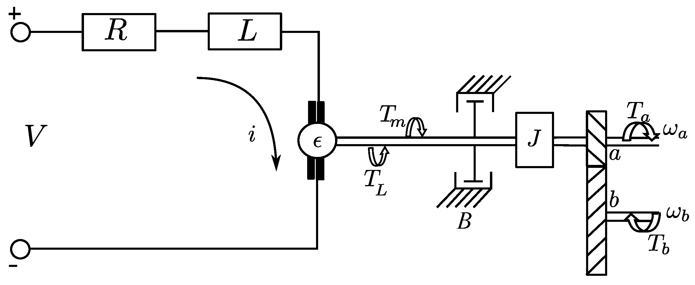
2.2. Mathematical Model of the Electric Motor and Transmission

In Figure 2, a schematic diagram of the electric motor is presented. The transmission ratio is

$$n=\frac{T_b}{T_a}=\frac{{\omega }_a}{{\omega }_b}$$

(21)

where ${\omega }_a$ and $T_a$ are the angular speed and the torque at the shaft a, respectively, ${\omega }_b$ is the angular velocity of the shaft b. $T_b$ is the system-delivered torque and is equal to T in Equation (1).

By using Kirchoff’s voltage law we obtain

$$V_a=Ri\left(t\right)+L\dot{i}\left(t\right)+e$$

(22)

where $V_a$ is the input voltage to the motor–gear system, R is the motor’s armature resistance, L is the motor inductance, $i\left(t\right)$ is the current, and e is the electromotive force generated by the motor. The applied torques in the motor and gear are expressed as

$$T=n(T_m-T_L-B{\omega }_a-J{\dot{\omega }}_a)$$

(23)

where $T_m$ represents the motor electromagnetic torque and n is the transmission ratio defined in Equation (21).

The magnetic torque and the back electromotive force are defined as

$$\begin{array}{c}{T}_m=K_{m}i\left(t\right)\end{array}$$

(24)

$$\begin{array}{c}e=K_g{\omega }_a\end{array}$$

(25)

where $K_m$ and $K_g$ represent the torque and voltage parameters of the motor.

Since the shaft b gives propulsion to the crank mechanism, (21) can be written as:

$${\omega }_a=n{\omega }_b=n{\dot{\varphi }}_2$$

(26)

From (22)–(26), the mathematical model of the motor is obtained as

$$\begin{array}{cc}\hfill \dot{i}\left(t\right)& =\frac{1}{L}(V_a-Ri\left(t\right)-n{K}_g{\dot{\varphi }}_2)\hfill \end{array}$$

(27)

$$\begin{array}{cc}\hfill T& =n{K}_{m}i\left(t\right)-n{T}_L-n^{2}B{\dot{\varphi }}_2-n^{2}J{\ddot{\varphi }}_2\hfill \end{array}$$

(28)

2.3. Dynamic Model of the System

The potential and dissipative energies can be neglected in the mechanism since they are relatively small and the terms related to potential energy and due to the orientation of the mechanism. In this way, combining (20) and (28), the nonlinear equation of the system movement is

$$A\left({\varphi }_2\right){\ddot{\varphi }}_2+\frac{1}{2}\frac{dA\left({\varphi }_2\right)}{d{\varphi }_2}{\dot{\varphi }}_2^2=n{K}_{m}i\left(t\right)-n{T}_L-n^{2}B{\dot{\varphi }}_2-n^{2}J{\ddot{\varphi }}_2$$

(29)

From (27) and (29), it is possible to present the complete system model in state space as

$$\begin{array}{cc}\hfill \frac{d}{dt}\left(\frac{d{\varphi }_2}{dt}\right)& =A_0\left[A_1{\left(\frac{d{\varphi }_2}{dt}\right)}^2+A_2\frac{d{\varphi }_2}{dt}+n{K}_{m}i+A_3\right]\hfill \end{array}$$

(30)

$$\begin{array}{cc}\hfill \frac{di}{dt}& =\frac{1}{L}\left(V_a-Ri-n{K}_g\frac{d{\varphi }_2}{dt}\right)\hfill \end{array}$$

(31)

where

$$\begin{array}{cc}\hfill A_0& =\frac{1}{A\left({\varphi }_2\right)+n^{2}J}\hfill \\ \hfill A_1& =-\frac{1}{2}\frac{A\left({\varphi }_2\right)}{{\varphi }_2}\hfill \\ \hfill A_2& =-n^{2}B\hfill \\ \hfill A_3& =-n{T}_L\hfill \end{array}$$

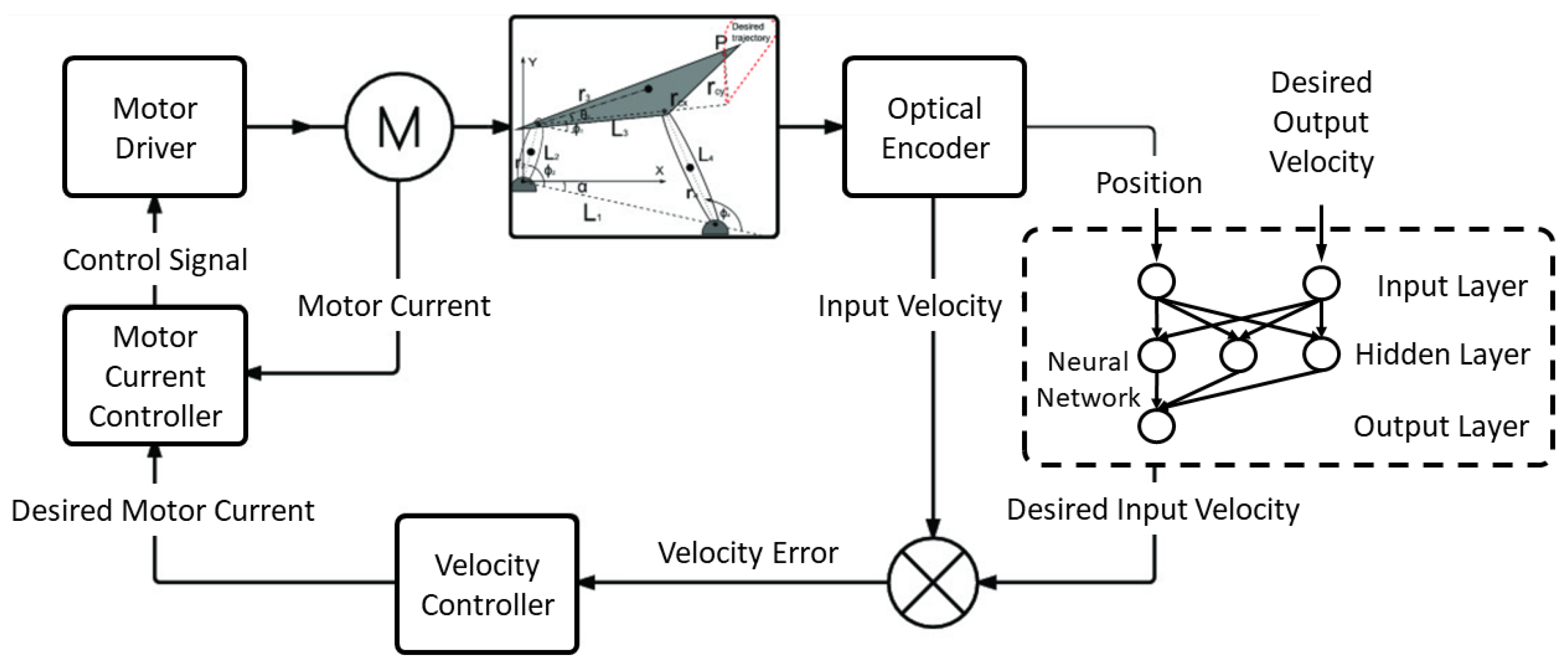
3. ANN-Based PID Control Scheme

The control scheme described in this work consists of two stages. The first one obtains the current reference ($i_a$), which is a virtual control signal as a function of the velocity error. The second stage determines the armature voltage applied to the motor ($v_a$), which is necessary to achieve the desired coupler point velocity. Linearization via feedback and a PID controller are applied in both control loops to assure the correct velocity regulation in the coupler point. It is important to highlight that for each point of the trajectory, it is necessary to solve the kinematic model for the crank velocity for the coupler point motion to reach the desired speed. A neural network estimator is used for this task as a variable velocity drive estimator. The complete control scheme is presented in Figure 3.

3.1. Current Control Loop

To synthesize the control law for the motor current, the tracking error is defined as $e_i=i-i^{\ast }$. Taking into account (31), the error dynamics ${\displaystyle \frac{d{e}_i}{dt}}$ can be written as

$${\displaystyle \frac{d{e}_i}{dt}}=\frac{1}{L}\left(V_a-Ri-n{k}_g\dot{{\varphi }_2}\right)-{\displaystyle \frac{d{i}^{\ast }}{dt}}.$$

(32)

From (32), a linearizing PID control signal can be proposed as follows:

$$V_a=Ri+n{k}_g\dot{{\varphi }_2}+L{\displaystyle \frac{d{i}^{\ast }}{dt}}-L\left(k_p{e}_i+k_i\eta +k_d{\displaystyle \frac{d{e}_i}{dt}}\right)$$

(33)

where

$${\displaystyle \frac{d\eta }{dt}}=e_i$$

Introducing the control law (33) into the error dynamics (32), we obtain

$$\begin{array}{cc}\hfill {\displaystyle \frac{d{e}_i}{dt}}& =-k_p{e}_i-k_i\eta -k_d{\displaystyle \frac{d{e}_i}{dt}}\hfill \\ \hfill & =-\frac{k_p{e}_i+k_i\eta }{1+k_d}\hfill \end{array}$$

(34)

where the error dynamics can be globally asymptotically stable if the gains $k_p$, $k_i$, and $k_d$ are adequately selected.

3.2. Velocity Control Loop

As can be noted, the control law (33), includes the current reference ($i^{\ast }$) and its time derivative. To calculate this reference signal, we design the second control loop where we must consider the velocity tracking error, defined as $e_v=\dot{{\varphi }_2}-{\dot{{\varphi }_2}}^{\ast }$, where ${\dot{{\varphi }_2}}^{\ast }$ is the reference velocity. Considering (30), the velocity error dynamics can be written as

$${\displaystyle \frac{d{e}_v}{dt}}=A_0\left(A_1{\dot{{\varphi }_2}}^2+A_2\dot{{\varphi }_2}+n{K}_{m}i+A_3\right)-{\displaystyle \frac{d}{dt}}{\dot{{\varphi }_2}}^{\ast }.$$

(35)

Replacing i with $e_i+i^{\ast }$,

$${\displaystyle \frac{d{e}_v}{dt}}=A_0\left(A_1{\dot{{\varphi }_2}}^2+A_2\dot{{\varphi }_2}+n{K}_m(e_i+i^{\ast })+A_3\right)-{\displaystyle \frac{d}{dt}}{\dot{{\varphi }_2}}^{\ast }.$$

(36)

Taking into account that the first control loop ensures that $e_i\to 0$ in short time, (36) is reduced to

$${\displaystyle \frac{d{e}_v}{dt}}=A_0\left(A_1{\dot{{\varphi }_2}}^2+A_2\dot{{\varphi }_2}+n{K}_m{i}^{\ast }+A_3\right)-{\displaystyle \frac{d}{dt}}{\dot{{\varphi }_2}}^{\ast }.$$

(37)

As $i^{\ast }$ is considered a virtual control signal, it can be proposed as

$$i^{\ast }=-{\displaystyle \frac{1}{n{k}_m}}\left(A_1{\dot{{\varphi }_2}}^2+A_2\dot{{\varphi }_2}+A_3+{\displaystyle \frac{k_{p2}{e}_v+k_{i2}\xi +k_{d2}{\displaystyle \frac{d{e}_v}{dt}}-{\displaystyle \frac{d}{dt}}{\dot{{\varphi }_2}}^{\ast }}{A_0}}\right),$$

(38)

where

$$\dot{\xi }=e_v.$$

Then, replacing the control law (38) into the velocity error dynamics (37), we obtain

$$\begin{array}{cc}\hfill d{\displaystyle \frac{e_v}{dt}}& =-k_{p2}{e}_v-k_{i2}\xi -k_{d2}d{\displaystyle \frac{e_v}{dt}}\hfill \\ \hfill & =-\frac{k_{p2}{e}_v+k_{i2}\xi }{1+k_{d2}}.\hfill \end{array}$$

(39)

To verify the stability of the complete closed loop system, a Lyapunov candidate function is proposed as

$$W\left(z\right)=z^{T}Kz>0$$

(40)

where

$$z={\left[e_i,e_v,\eta ,\xi \right]}^T$$

and

$$K=\left[\begin{array}{cccc}1+k_{d2}& 0& 1+k_{d2}& 0\\ 0& 1+k_d& 0& 1+k_d\\ 1+k_{d2}& 0& k_{p2}+k_{i2}& 0\\ 0& 1+k_d& 0& k_p+k_i\end{array}\right]$$

Selecting $k_p+k_i>1+k_d>0$ and $k_{p2}+k_{i2}>1+k_{d2}>0$, we can guarantee that the matrix K is positive definite.

Then, if $\dot{W}\left(z\right)<0\forall z\in \mathbb{R}-\left\{0\right\}$, the global and asymptotically stability condition of the system is demonstrated. So, this time derivative can be written as follows:

$$\begin{array}{ccc}\dot{W}\left(z\right)\hfill & =& {\dot{z}}^{T}Kz\hfill \\ \hfill & =& -\left(k_{p2}-k_{d2}-1\right)e_i^2-\left(k_p-k_d-1\right)e_v^2-k_{i2}{\xi }^2-k_i{\eta }^2\hfill \end{array}$$

The above result satisfies the stability condition if $k_p>1+k_d$, $k_{p2}>1+k_{d2}$, $k_i>0$, and $k_{i2}>0$, then the origin of the error dynamics of the complete closed loop system is the unique stability point, and is global and asymptotically stable.

It is important to remark that in the stability proof, the error $e_i=i-i^{\ast }$ was not explicitly included because it is identical to the variable $\xi$.

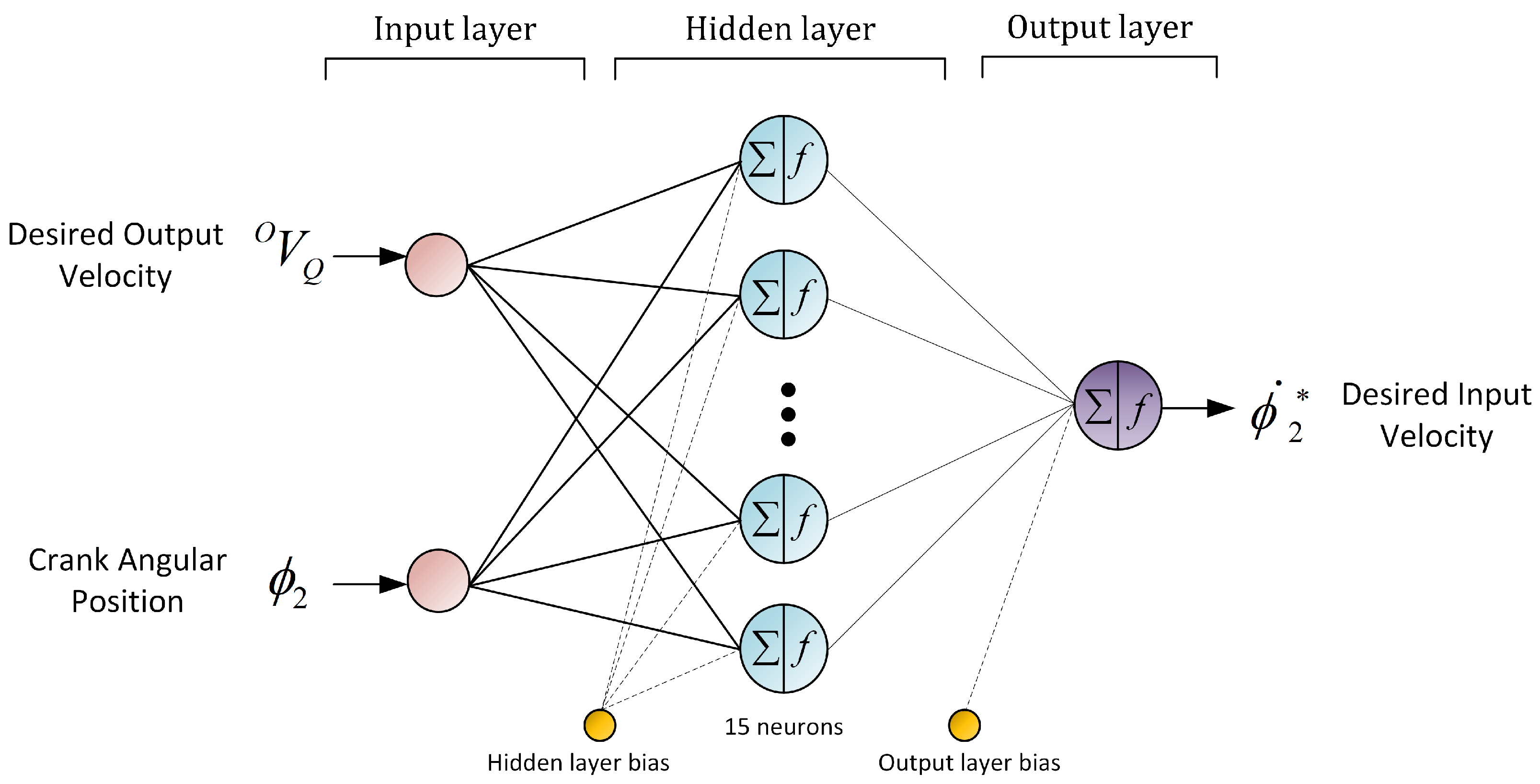
3.3. Variable Input Velocity Generator with Artificial Neural Networks (ANNs)

To determine the velocity reference ${\dot{{\varphi }_2}}^{\ast }$ at which the crank must rotate so that the coupler point Q reaches the desired velocity, we first establish a kinematics model for the four-bar mechanism.

The description of the position of ${}^O\mathbf{Q}$ with respect to the global reference system $\{X-Y\}$, from Figure 1, is given by

$${}^O\mathbf{Q}={\mathbf{r}}_0+R{(\widehat{z},\alpha )}^r\mathbf{Q}$$

(41)

where ${}^r\mathbf{Q}$ represents the position of the point Q measured with respect the local reference system, ${\mathbf{r}}_0$ represents the translation, and $R(\widehat{z},\alpha )$ corresponds to the canonical rotation matrix of an angle $\alpha$ around the $\widehat{z}$ axis, between the local reference system $\{x_r-y_r\}$ and the global $\{X-Y\}$. This can be expanded as

$${}^O\mathbf{Q}=\left[\begin{array}{c}{}^0{Q}_x\\ {}^0{Q}_y\end{array}\right]=\left[\begin{array}{c}{x}_0+L_{2}cos({\varphi }_2+\alpha )+r_{cx}cos({\varphi }_3+\alpha )-r_{cy}sin({\varphi }_3+\alpha )\\ y_0+L_{2}sin({\varphi }_2+\alpha )+r_{cx}sin({\varphi }_3+\alpha )+r_{cy}cos({\varphi }_3+\alpha )\end{array}\right]$$

(42)

The linear velocity of the point ${}^O\mathbf{Q}$ is obtained from the derivate of Equation (42) as

$${}^O{\mathbf{V}}_Q=\left[\begin{array}{c}{}^0{V}_x\\ {}^0{V}_y\end{array}\right]=\left[\begin{array}{c}-L_{2}sin({\varphi }_2+\alpha ){\dot{\varphi }}_2-r_{cx}sin({\varphi }_3+\alpha ){\dot{\varphi }}_3-r_{cy}cos({\varphi }_3+\alpha ){\dot{\varphi }}_3\\ L_{2}cos({\varphi }_2+\alpha ){\dot{\varphi }}_2+r_{cx}cos({\varphi }_3+\alpha ){\dot{\varphi }}_3-r_{cy}sin({\varphi }_3+\alpha ){\dot{\varphi }}_3\end{array}\right]$$

(43)

The function of the linear input velocity profile is defined as

$${\Vert }^O{\mathbf{V}}_Q\Vert =\sqrt{{}^0{V}_x^2{+}^0{V}_y^2}$$

(44)

The desired angular velocity profile function is given by

$${\dot{\varphi }}_2=\frac{\sqrt{{}^0{V}_x^2{+}^0{V}_y^2}}{\lambda }$$

(45)

where

$${\lambda }^2=L_2^2+r_{cx}^2{\gamma }^3+r_{cy}^2{\gamma }^3+2L_2{\gamma }_3[r_{cx}cos({\varphi }_2-{\varphi }_3)+r_{cy}sin({\varphi }_2-{\varphi }_3)]$$

To reduce the computational burden in the numerical solution of (45), when estimating ${\dot{\varphi }}_2^{\ast }$ we train an artificial neural network feed with the measured crank angular position ${\varphi }_2$ and the desired output velocity ${}^O{\mathbf{V}}_Q$. Computational intelligence methods have been successfully integrated with control schemes to relax the requirement of knowledge of the system model, consider uncertainties, and incorporate performance criteria. In particular, Artificial Neural Networks (ANNs) are attractive due to their nonlinear function approximation capabilities and simplicity of design and implementation.

A neural network generates a function approximation through a training process. The ANN is composed of an input layer with m inputs, a hidden neurons layer with N neurons, and an output layer with one single neuron as shown in Figure 4. Each hidden neuron is fully connected to the inputs and neurons in the output layer via the adaptable weights $w_{Ok}$ and $w_{I\left(k,m\right)}$, and $b_m$ and $b_O$ are the bias terms for each neuron. The function $\phi$ is known as the activation function and is usually a sigmoid. In feedforward networks, the learning algorithm is based on retro-propagation of the approximation error which adapts each weight in the network [32].

$$\begin{array}{cc}\hfill y& =\sum _{k=1}^N\left[w_{Ok}·\phi \left(\sum _{m=1}^M{w}_{I\left(k,m\right)}·x_m+b_m\right)+b_O\right]\hfill \\ \hfill \phi \left(x\right)& =\frac{1}{1+e^{-x}}\hfill \end{array}$$

(46)

In this study, a two-layer feed-forward neural network with fifteen neurons in its hidden layer was designed. The data to build the neural net were taken by turning the crank at various velocities; the velocity, the coupler point velocity, and the angular position of both were recorded. To adjust the neural network, the crank’s angular position and the coupler point’s velocity are used as input data; the output data point is the crank velocity. Of the 46 simulation runs under different velocity profiles, 16,560 samples constituted the data set where $70\%$ was used for training, $15\%$ for validation, and $15\%$ for testing. The training algorithm used was Bayesian regularization and the number of epochs is fixed at 1000, with a fitness calculated as $R^2=99.99\%$ and a medium square error $MSE=0.000372$ as displayed in Figure 4.

4. Simulation Results and Discussion

To verify the performance of the proposed control scheme, several simulations in closed-loop were performed. The first simulation applies the state space model of the four-bar mechanism with a PID controller and constant crank velocity. The second test presents the proposed control scheme with a variable input velocity to obtain a constant output velocity at the coupler point. The third experiment presents the proposed control scheme with a variable input velocity, but in this case, it generates two different output velocities at the coupler point. These tests are intended to demonstrate the advantages of the proposed control scheme compared with [28].

4.1. Servo-Controlled Four-Bar Mechanism Simulation Parameters

The parameters of the simulated servo-controlled four-bar mechanism are detailed in

Table 2. Mechanism Parameters.

Parameter	Value
$L_1$ (m)	0.3972
$L_2$ (m)	0.0588
$L_3$ (m)	0.2351
$L_4$ (m)	0.22716
$r_{cx}$ (m)	0.403779
$r_{cy}$ (m)	0.093921
$J_2$ (kg·m${}^2$)	$2.76\times {10}^{-5}$
$J_3$ (kg·m${}^2$)	$3.5468\times {10}^{-3}$
$J_4$ (kg·m${}^2$)	$\mathrm{3.8779}\mathrm{\times }{\mathrm{10}}^{\mathrm{-}\mathrm{4}}$
m${}_2$ (kg)	0.04234
m${}_3$ (kg)	0.2586
m${}_4$ (kg)	0.08156
$\alpha$ (rad)	5.83047

and

Table 3. Motor Parameters.

Parameter	Value
R ($\mathsf{\Omega }$)	2
L(H)	1
$K_m$ (N·m/A)	0.260
$K_g$ (V·s)	0.260
J (kg·m${}^2$)	0.011
$T_L$ (N·m)	0.28
B (N·m·s)	0

. The resulting path of the coupler point for this mechanism is shown in Figure 5. As can be seen, this path has two linear sections followed by two curved segments, the upper one is smooth and the lower one is more demanding. This behavior demonstrates that the relationship between the velocity of the crank and the velocity of the coupler point is nonlinear since the displacements are different, even if the angular movement is the same. Hence, some points the trajectory generated by the coupler point of the four-bar mechanism have a complex geometric trajectory that will cause abrupt changes in the velocity direction. Therefore, one complex trajectory and the required constant speed profile of the coupler point during the whole trajectory, and limit positions for the output link, evidently will generate speed fluctuations that the controller has to overcome in order to fulfil the task.

4.2. Constant Crank Velocity

The test consists of regulating the crank angular velocity of the mechanism at $5$ rad/s ($47.74$ rpm) by means of the PID controller presented in [29]. The controller gains are given in

Table 4. Controller Gains.

Parameter	Value
$K_p$	3000
$K_d$	200
$K_i$	50
$K_{p2}$	10.8
$K_{d2}$	0
$K_{i2}$	100

. As observed in Figure 6a, the crank angular velocity is regulated with a maximum error of 0.02 rad/s, and the convergence time is $0.05$ s (at ${15}^{\circ }$). In addition, Figure 6b shows that the velocity of the coupler point is variable all the time during the trajectory of the mechanism. As previously mentioned, this is the traditional control task for this mechanism; however, the coupler point is where the work is performed, so it is important to control its velocity at a desired value.

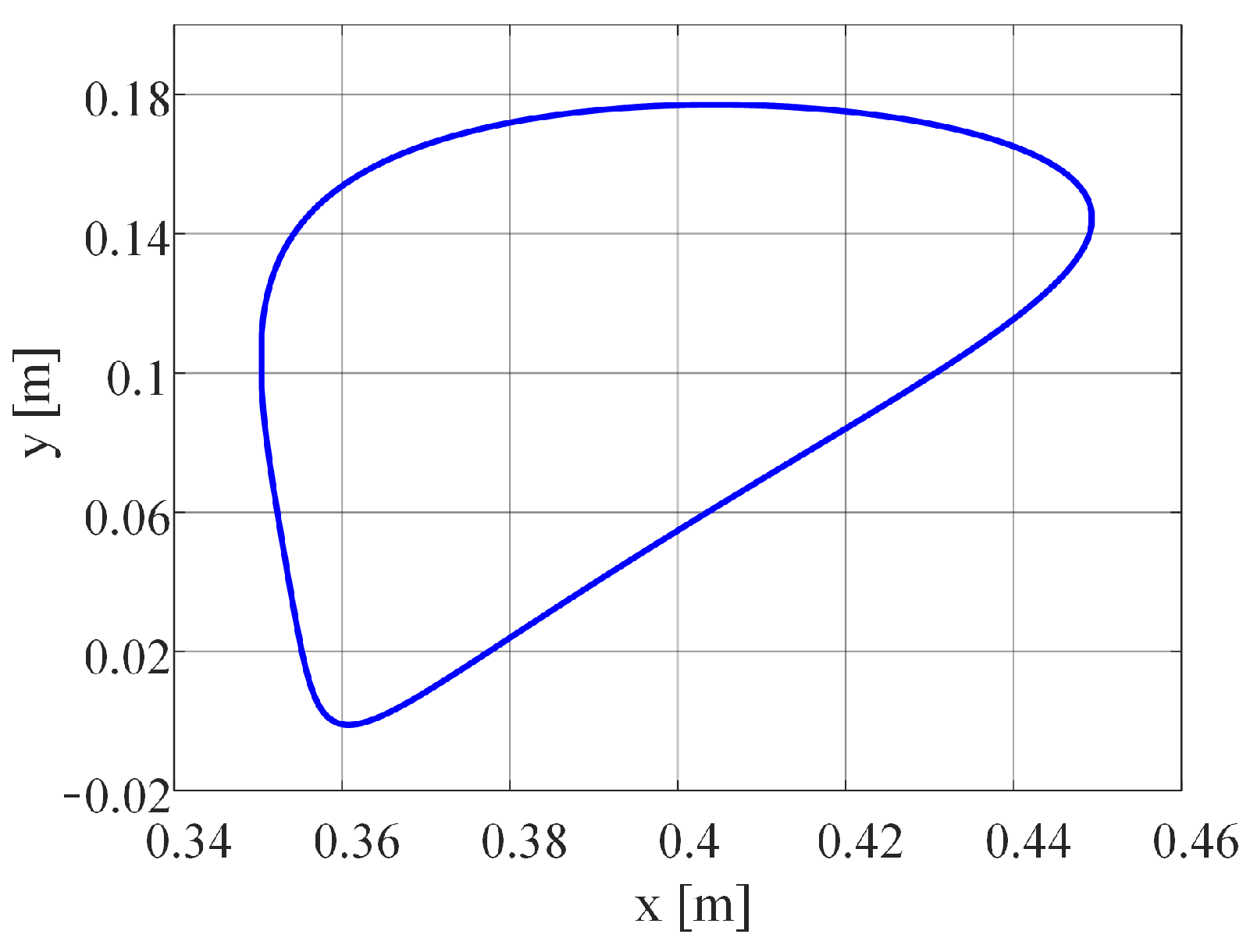
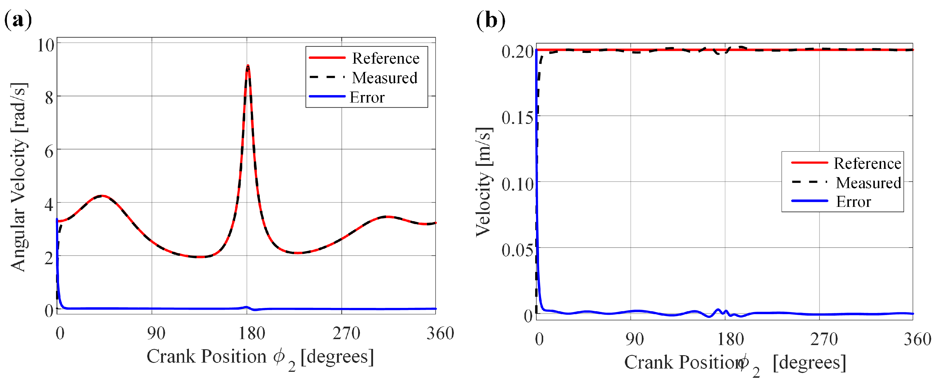
4.3. Variable Input Velocity for Obtaining a Constant Output Velocity at the Coupler Point

This test is carried out to show that the proposed control scheme allows for indirect regulation of the velocity of the coupler point by fulfilling two requirements. Firstly, the reference crank velocity, obtained through the developed neural network, is close to the real value; additionally, the proposed control tracks this reference with minimal error. In this case, a velocity of 0.2 m/s is imposed for the coupler point. In Figure 7a it is noted that there is an excellent tracking of the desired trajectory, since the convergence time is 0.02 s (at $8^{\circ }$) and the maximum error is 0.07 rad/s. The previous result makes it possible to regulate the velocity of the coupler point at the desired value, as shown in Figure 7b. Note that the coupler point velocity error is less than 0.003 m/s and the convergence time is 0.02 s, which is consistent with that of the angular velocity of the crank presented in Figure 7a.

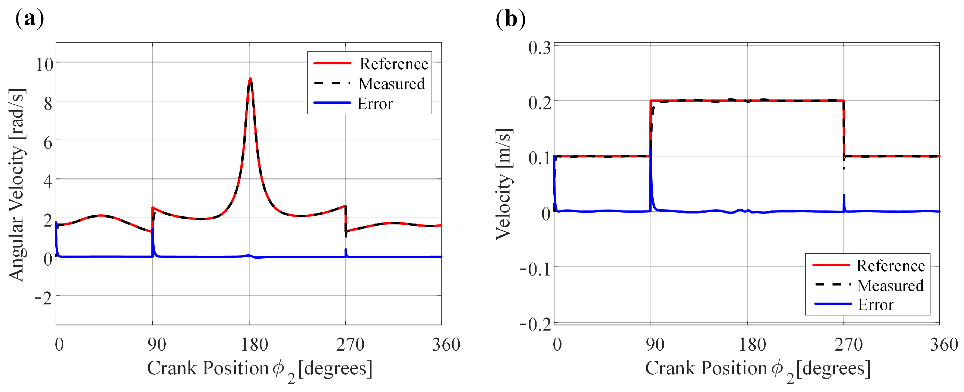
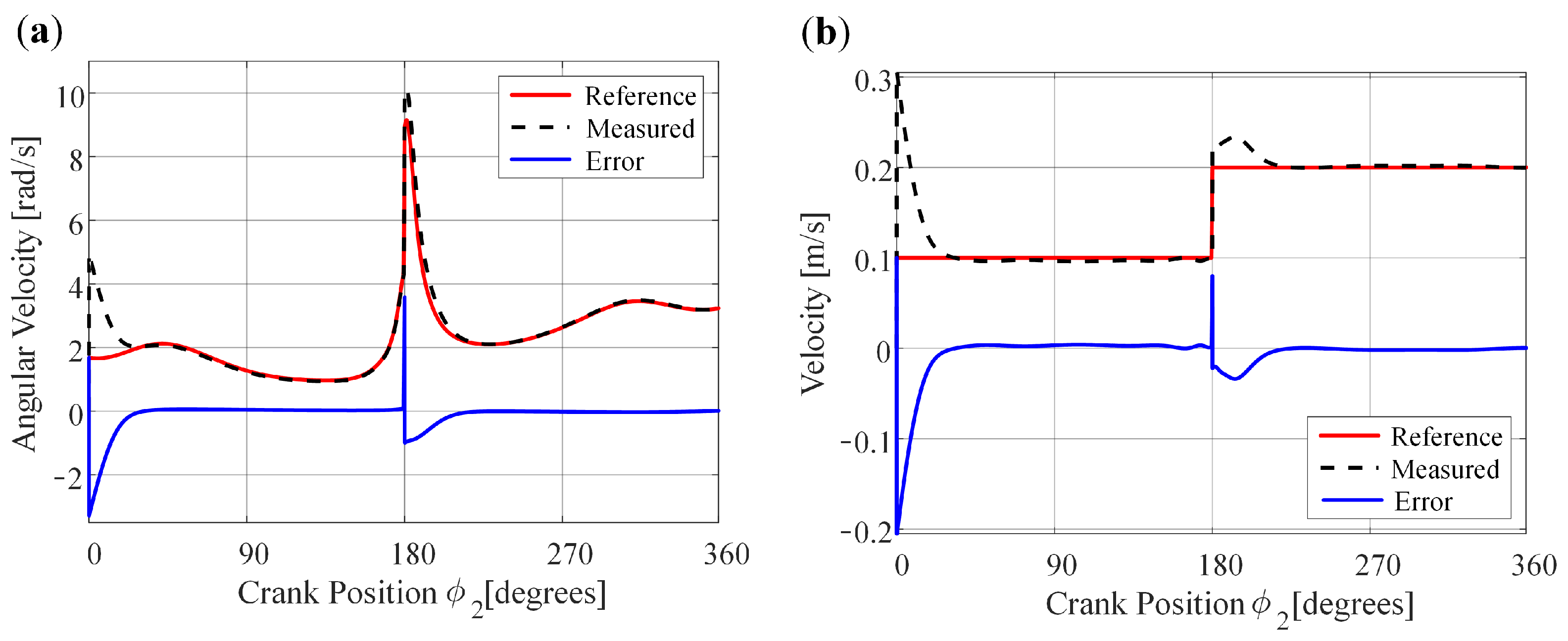
4.4. Variable Input Velocity for Generating Two Different Output Velocities at the Coupler Point

In real applications, the coupler point is not required to carry out its entire travel with a constant velocity, but rather to have a specific velocity in the segment in which it performs the work and a different velocity for the return. For this reason, the experiment is carried out when a more complex velocity profile is imposed on the coupler point. As displayed in Figure 8a, the angular crank velocity reference has abrupt changes at $90{}^{\circ }$ and $270{}^{\circ }$. These are needed to regulate the coupler point velocity to the conditions

$$V_Q=\left\{\begin{array}{cc}0.2\mathrm{m}/\mathrm{s}\hfill & {90}^{\circ }\le {\varphi }_2<{270}^{\circ }\\ 0.1\mathrm{m}/\mathrm{s}\hfill & \mathrm{otherwise}.\end{array}\right.$$

(47)

In Figure 8b, the coupler point velocity error is less than 0.003 m/s and the convergence time is 0.02 s, which are the same as the presented in Section 4.3 for the coupler point.

A more severe test is the one that implies that the velocity changes of the coupler point are where the control is most demanded, this happens when ${\varphi }_2={180}^{\circ }$, which is where the most abrupt change would occur. In this test, the velocity profile that is imposed on the coupler point is

$$V_Q=\left\{\begin{array}{cc}0.2\mathrm{m}/\mathrm{s}\hfill & {180}^{\circ }\le {\varphi }_2<{360}^{\circ }\\ 0.1\mathrm{m}/\mathrm{s}\hfill & \mathrm{otherwise}.\end{array}\right.$$

(48)

Figure 9a shows the tracking of the crank velocity reference, this is fast and with minimum error. In Figure 9b, the change of velocity at the coupler point is presented. In this case, the convergence time is 0.0266 s (at ${20}^{\circ }$) and the maximum error is 0.03 m/s. It can be emphasized that this would be the worst case for this mechanism; in spite of that, the system is controlled at the desired velocity at the specified points.

It is important to indicate that the saturation function was used in the simulation to prevent $V_a$ from increasing to values that could cause some damage to the system; however, it was observed that in all the cases presented, such voltage did not reach the saturation limits. To exhibit this performance, Figure 10 shows the input voltage to the motor corresponding to the input profiles defined by (47) and (48), and the results are shown in Figure 8 and Figure 9.

In summary, the designed controller achieved trajectory tracking with good performance both on tracking error and transient response. The proposed control scheme has a simple structure and low computational burden for real-time applications. In the case when more demanding performance is required, then the computational intelligence methods can be integrated with other high-performance algorithms such as the type-2 fuzzy presented in [25,26,27] which can deliver exact responses and robustness.

5. Conclusions

In this work, the problem of controlling a four-bar mechanism for the case of variable velocity of the crank is considered. To obtain the desired output motions for the coupler point, an indirect control is designed to estimate the reference values for the motor current to achieve trajectory tracking for each crank velocity profile. Furthermore, a neural network is introduced in the control scheme to solve the kinematic model of the mechanism to obtain the velocity reference. The controlled system is tested through simulations under several trajectories, obtaining excellent results. Further research will implement the four-bar mechanism with the proposed controller using an optical encoder and or computer vision for the position feedback.

References

1. Tao, J.; Sadler, J. Constant speed control of a motor driven mechanism system. Mech. Mach. Theory 1995, 30, 737–748. [Google Scholar] [CrossRef]
2. Dulger, L.; Uyan, S. Modelling, simulation and control of a four-bar mechanism with a brushless servo motor. Mechatronics 1997, 7, 369–383. [Google Scholar] [CrossRef]
3. Li, Q.; Tso, S.; Guo, L.; Zhang, W. Improving motion tracking of servomotor-driven closed-loop mechanisms using mass-redistribution. Mech. Mach. Theory 2000, 35, 1033–1045. [Google Scholar] [CrossRef]
4. Wu, F.X.; Zhang, W.J.; Li, Q.; Ouyang, P.R. Integrated Design and PD Control of High-Speed Closed-loop Mechanisms. J. Dyn. Syst. Meas. Control 2002, 124, 522–528. [Google Scholar] [CrossRef]
5. Su, Y.; Sun, D.; Zheng, C. Nonlinear trajectory tracking control of a closed-chain manipulator. In Proceedings of the Fifth World Congress on Intelligent Control and Automation (IEEE Cat. No. 04EX788), Hangzhou, China, 15–19 June 2004; Volume 6, pp. 5012–5016. [Google Scholar] [CrossRef]
6. Lin, M.C.; Chen, J.S. Experiments toward MRAC design for linkage system. Mechatronics 1996, 6, 933–953. [Google Scholar] [CrossRef]
7. Gündoğdu, Ö.; Erentürk, K. Fuzzy control of a dc motor driven four-bar mechanism. Mechatronics 2005, 15, 423–438. [Google Scholar] [CrossRef]
8. Koca, G.O.; Akpolat, Z.H.; Özdemir, M. Type-2 Fuzzy Sliding Mode Control of A Four-Bar Mechanism. Int. J. Model. Simul. 2011, 31, 60–68. [Google Scholar] [CrossRef]
9. Hwang, C.L.; Kuo, C.Y. A stable adaptive fuzzy sliding-mode control for affine nonlinear systems with application to four-bar linkage systems. IEEE Trans. Fuzzy Syst. 2001, 9, 238–252. [Google Scholar] [CrossRef]
10. Koca, G.O.; Akpolat, Z.H.; Özdemir, M. Development of robust fuzzy control methods and their applications to a mechanical system. Turk. J. Sci. Technol. 2014, 9, 47–56. [Google Scholar]
11. Ren, Q.; Bigras, P. Design and implementation of model-free PID fuzzy logic control on a 4-bar parallel mechanism. In Proceedings of the 2015 IEEE International Conference on Advanced Intelligent Mechatronics (AIM), Busan, Republic of Korea, 7–11 July 2015; pp. 1647–1652. [Google Scholar] [CrossRef]
12. Zhang, Y.; Feng, C.; Li, B. PID Control of Nonlinear Motor-Mechanism Coupling System Using Artificial Neural Network. In Advances in Neural Networks—ISNN 2006, Proceedings of the Third International Symposium on Neural Networks, Chengdu, China, 28 May–1 June 2006; Wang, J., Yi, Z., Zurada, J.M., Lu, B.L., Yin, H., Eds.; Springer: Berlin/Heidelberg, Germany, 2006; pp. 1096–1103. [Google Scholar]
13. Lungu, R.; Sepcu, L.; Lungu, M. Four-Bar Mechanism’s Proportional-Derivative and Neural Adaptive Control for the Thorax of the Micromechanical Flying Insects. J. Dyn. Syst. Meas. Control 2015, 137, 051005. [Google Scholar] [CrossRef]
14. Çakar, O.; Tanyıldızı, A.K. Application of moving sliding mode control for a DC motor driven four-bar mechanism. Adv. Mech. Eng. 2018, 10, 1687814018762184. [Google Scholar] [CrossRef]
15. Salah, M.; Al-Jarrah, A.; Tatlicioglu, E.; Banihani, S. Robust Backstepping Control for a Four-Bar Linkage Mechanism Driven by a DC Motor. J. Intell. Robot. Syst. 2019, 94, 327–338. [Google Scholar] [CrossRef]
16. Erenturk, K. Hybrid Control of a Mechatronic System: Fuzzy Logic and Grey System Modeling Approach. IEEE/ASME Trans. Mechatronics 2007, 12, 703–710. [Google Scholar] [CrossRef]
17. Al-Jarrah, A.; Salah, M.; Banihani, S.; Al-Widyan, K.; Ahmad, A. Applications of Various Control Schemes on a Four-Bar Linkage Mechanism Driven by a Geared DC Motor. WSEAS Trans. Syst. Control 2015, 10, 584–597. [Google Scholar]
18. Tutunji, T.A.; Salah, M.; Al-Jarrah, A.; Ahmad, A.; Alhamdan, R. Modeling and Identification of a Four-Bar Linkage Mechanism Driven by a Geared DC Motor. Int. Rev. Mech. Eng. 2015, 9, 296–306. [Google Scholar] [CrossRef]
19. İşbitirici, A.; Altuğ, E. Design and Control of a Mini Aerial Vehicle that has Four Flapping-Wings. J. Intell. Robot. Syst. 2017, 88, 247–265. [Google Scholar] [CrossRef]
20. Mohseni, S.A.; Duchaine, V.; Wong, T. A comparative study of the optimal control design using evolutionary algorithms: Application on a close-loop system. In Proceedings of the 2017 Intelligent Systems Conference (IntelliSys), London, UK, 7–8 September 2017; pp. 942–948. [Google Scholar] [CrossRef]
21. Rodríguez-Molina, A.; Villarreal-Cervantes, M.G.; Aldape-Pérez, M. Indirect adaptive control using the novel online hypervolume-based differential evolution for the four-bar mechanism. Mechatronics 2020, 69, 102384. [Google Scholar] [CrossRef]
22. Shi, K.; Liu, C.; Sun, Z.; Yue, X. Coupled orbit-attitude dynamics and trajectory tracking control for spacecraft electromagnetic docking. Appl. Math. Model. 2022, 101, 553–572. [Google Scholar] [CrossRef]
23. Liu, C.; Yue, X.; Shi, K.; Sun, Z. Spacecraft Attitude Control: A Linear Matrix Inequality Approach; Elsevier: London, UK, 2022. [Google Scholar] [CrossRef]
24. Perrusquía, A.; Flores-Campos, J.A.; Yu, W. Optimal sliding mode control for cutting tasks of quick-return mechanisms. ISA Trans. 2022, 122, 88–95. [Google Scholar] [CrossRef]
25. Hua, G.; Wang, F.; Zhang, J.; Alattas, K.A.; Mohammadzadeh, A.; The Vu, M. A New Type-3 Fuzzy Predictive Approach for Mobile Robots. Mathematics 2022, 10, 3186. [Google Scholar] [CrossRef]
26. Xu, S.; Zhang, C.; Mohammadzadeh, A. Type-3 Fuzzy Control of Robotic Manipulators. Symmetry 2023, 15, 483. [Google Scholar] [CrossRef]
27. Mohammadzadeh, A.; Sabzalian, M.H.; Ahmadian, A.; Nabipour, N. A dynamic general type-2 fuzzy system with optimized secondary membership for online frequency regulation. ISA Trans. 2021, 112, 150–160. [Google Scholar] [CrossRef]
28. Yan, H.S.; Yan, G.J. Integrated control and mechanism design for the variable input-speed servo four-bar linkages. Mechatronics 2009, 19, 274–285. [Google Scholar] [CrossRef]
29. Peón-Escalante, R.; Flota-Bañuelos, M.; Ricalde, L.J.; Acosta, C.; Perales, G.S. On the coupler point velocity control of variable input speed servo-controlled four-bar mechanism. Adv. Mech. Eng. 2016, 8, 1687814016678356. [Google Scholar] [CrossRef]
30. Flota-Bañuelos, M.; Peón-Escalante, R.; Ricalde, L.J.; Cruz, B.J.; Quintal-Palomo, R.; Medina, J. Vision-based control for trajectory tracking of four-bar linkage. J. Braz. Soc. Mech. Sci. Eng. 2021, 43. [Google Scholar] [CrossRef]
31. Goldstein, H.; Poole, C.; Safko, J. Classical Mechanics; Pearson Education: London, UK, 2011. [Google Scholar]
32. Haykin, S.S. Neural Networks and Learning Machines; Prentice Hall: London, UK, 2016. [Google Scholar]
Figure 1. Schematic of four-bar linkage.
Mathematics 11 02148 g001
Figure 2. Schematic diagram of the motor and transmission.
Mathematics 11 02148 g002
Figure 3. ANN-based control scheme for variable input velocity tracking of four-bar mechanism.
Mathematics 11 02148 g003
Figure 4. Neural network estimator for the input velocity Feedforward architecture.
Mathematics 11 02148 g004
Figure 5. Path of the coupler point of the mechanism.
Mathematics 11 02148 g005
Figure 6. Simulation results of constant crank velocity with PID Control. (a) Crank angular velocity. (b) Coupler point velocity.
Mathematics 11 02148 g006
Figure 7. Variable input velocity for obtaining a constant output velocity at the coupler point. (a) Crank angular velocity. (b) Coupler point velocity.
Mathematics 11 02148 g007
Figure 8. Variable input velocity for generating two different output velocities at the coupler point. (a) Crank angular velocity. (b) Coupler point velocity.
Mathematics 11 02148 g008
Figure 9. Variable input velocity for generating two different output velocities at the coupler point. (a) Crank angular velocity. (b) Coupler point velocity.
Mathematics 11 02148 g009
Figure 10. Variable input velocity for generating two different output velocities at the coupler point. (a) V Q described in Equation (47). (b) V Q described in Equation (48).
Mathematics 11 02148 g010