
Analysis and Consequences on Some Aggregation Functions of PRISM (Partial Risk Map) Risk Assessment Method


1
Department of Management and Business Economics, Budapest University of Technology and Economics, H-1117 Budapest, Hungary
2
Department of Supply Chain Management, University of Pannonia, H-8200 Veszprém, Hungary
*
Author to whom correspondence should be addressed.
Mathematics 2022, 10(5), 676; https://doi.org/10.3390/math10050676
Submission received: 22 January 2022
/
Revised: 13 February 2022
/
Accepted: 19 February 2022
/
Published: 22 February 2022
(This article belongs to the Special Issue Mathematical Methods and Operation Research in Logistics, Project Planning, and Scheduling)
Abstract
:The PRISM (partial risk map) methodology is a novel risk assessment method developed as the combination of the failure mode and effect analysis and risk matrix risk assessment methods. Based on the concept of partial risks, three different aggregation functions are presented for assessing incident risks. Since the different aggregation functions give different properties to the obtained PRISM numbers and threshold surfaces (convex, concave, linear), the description of these properties is carried out. Similarity analyses based on the sum of ranking differences (SRD) method and rank correlation are performed and robustness tests are applied related to the changes of the assessment scale lengths. The PRISM method provides a solution for the systematically criticized problem of the FMEA, i.e., it is not able to deal with hidden risks behind the aggregated RPN number, while the method results in an expressive tool for risk management. Applying new aggregation functions, proactive assessment can be executed, and predictions can be given related to the incidents based on the nature of their hidden risk. The method can be suggested for safety science environments where human safety, environmental protection, sustainable production, etc., are highly required.
Keywords:
partial risk map; PRISM; PRISM number; failure mode and effect analysis; FMEA; RPN; risk matrix; risk assessment; safety science; systems safetyMSC:
90B50; 90B251. Introduction
Nowadays, the development of risk assessment methodologies is clearly visible in the industry and service sector as well. One typical development direction is to combine different mathematical methodologies with a platform risk assessment methodology such as FMEA—failure mode and effect analysis [1,2], RM—risk matrix [3], HAZOP—hazard and operability analysis [4], FTA—fault tree analysis [5], etc. The typical aim of these studies is to develop the platform methodology, increasing its strengths and/or decreasing its weaknesses by adding new, typically mathematical features. Another major development direction is to combine a risk assessment methodology with another one [6,7,8]. Typically, the aim is to combine the strength of the risk assessment methodologies in this case. Throughout the decades of development, the reliability, effectiveness, usefulness, applicability, etc., of the platform risk assessment methodologies were significantly increased by dominantly mathematic-based methodological developments [9,10,11,12].
In our understanding, the risk is not just the probability of an incident but a composite of all the characteristics that are relevant to the incident and its possible outcome. In this paper, just the probability of the occurrence, the severity of the consequences, and the degree of undetectability are considered, but other aspects or features of the incident can be regarded as a component of the risk (e.g., criticality, range/expansion of the effects, controllability, etc.). The number of such characteristics that are considered can vary method by method; in most of the cases, these characteristics are described with values and condensed into a single value for each incident.
Based on the combination of the FMEA and RM methodologies, a novel risk assessment methodology called partial risk map (PRISM) was described. Although, the application of the methodology was presented in a case study related to the assessment of compliance risks in the banking sector [13], the PRISM risk assessment method is more generic and can be applied in different operational fields as well, where the risk assessment is based on similar rating factors to the FMEA, and the identification of hidden risks is essential. Thus, the method can be offered for safety science environments, where human health, environmental protection, and sustainable production are in the focus, and also applied to those fields, where the incident consequences can be generally high. Since the methodology is quite novel, it still has potential to improve in different descriptive, comparative, and developmental directions. Although, the methodology builds on the strengths of both the FMEA and RM methods, the mathematical process of the incident ranking is still not defined [13]. The purpose of this work is the mathematical development and description of the ranking algorithm of the PRISM method. The aim is to create, describe, and compare some aggregation functions for the incident characteristics to determine and to detail the application of the PRISM number. Since PRISM methodology applies the same risk assessment dimensions as FMEA, the paper also focuses on putting the results related to the PRISM number into the context of the RPN (risk priority number) of FMEA. Thus, the aim of the paper is to create the formal description of the theory of partial risks and to compare the newly developed formulas to each other and to the formula of RPN. The main results and innovations of the paper are the following:
- Three functions are developed for assessing partial risks (one algorithm is sensitive for incidents, having a high risk level at one rating factor, one algorithm is sensitive for middle risk levels at all the rating factors, one is a balanced algorithm). Applying the new functions, proactive assessment can be executed, and predictions can be given related to the incidents based on the nature of their hidden risk.
- The developed functions have an exact description based on the distribution of their possible values and these are compared to the distribution of RPN number.
- The rankings of the functions are compared to each other by applying different analyses, and detailed discussion of the theoretical differences is given based on the comparison.
- The rankings are robust related to the change of evaluation factor scales. This test is important, since, in the practical field, the evaluation scale lengths can be different.
Therefore, the work aims to identify the evaluation specialties of the different methods, and based on the comparisons, possible application suggestions are given for the practitioners and other research gaps are presented for future research and development.
Since the PRISM methodology builds off of some key specialties of FMEA and RM as well, in Section 1.1, a brief introduction of these two methodologies is given, and in Section 1.2, the description of the PRISM method is presented. All the methods featured in these subsections evaluate the risk of the incidents based on several risk factors and use some aggregation of these factors to provide an order of priority among the incidents. The applied method influences the priorities and directs the focus of risk mitigation in a different way.
1.1. Brief Description of the RM and FMEA
In this subsection, the focus is on the brief introduction of two methodologies, which have significant impacts on the aim of this study. Thus, RM and FMEA are introduced here since the PRISM method builds on some key features of these methodologies [14]. The introduction aims to describe the basic structures of the methods and to refer to some important notes of existing developments. There is no focus on the complete introduction of these methods, their practical applications, and all the consequences in the field of risk assessment techniques.
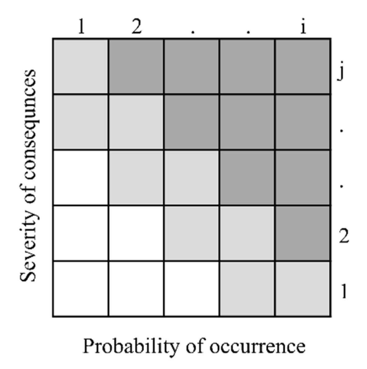
The methodology of the risk matrix is a widely applicable method of risk assessment. The structure of risk matrices is built up by factors developed to assess the risk of particular objects [15]. Risk matrices are usually based on two independent rating factors, which are the probability of occurrence and the severity of consequences [16]. In most cases, RM estimates the risk on ordinal or higher measurement scales having usually four to five different values. The higher the factor-related risk of the object, the higher the value of the factor.
The risk assessment is generally based on the score of the probability of occurrence and the severity of consequences factors [17]. In the case of having high values related to both rating factors, the associated risk is usually interpreted as high, while in the case of having low values related to the factors, the indicated risk level is low. However, other categories can be created as well. The visualization of the methodology is usually represented with a matrix as shown in Figure 1.
Selection of the set of the riskiest incidents that must be averted, mitigated, eliminated, etc., can be executed using a given or calculated threshold level. Once an aggregated value reaches the threshold level, it signals to the control system. In Figure 1, two threshold levels are visualized on the frontiers of the white, light gray, and dark gray cells as examples. The darker the region, the higher the priority.
Similar to the risk matrices, the failure mode and effect analysis methodology also estimates risks of certain incidents by different rating factors. In the case of FMEA, the estimation is based on the aggregation of three rating factor values (probability of occurrence, severity of consequences, and degree of undetectability). The most typical aggregation of these values is multiplication, as many scientific papers refer to it [1,2,18,19,20].
As for the result of the multiplication, the RPN can be calculated. Based on the RPN value, it can be decided whether any risk reduction action is necessary to be launched or not in case of certain incidents. Over the past decades, the RPN is widely criticized by scientists, highlighting a couple of weaknesses of the RPN.
One of the most criticized properties of the RPN is that some hidden or latent risks can be unestimated or misestimated because different combinations of the three factors can result in the same RPN [13,21,22,23,24,25]. Thus, these hidden risks can later lead to unexpected errors.
Despite structured criticisms [22,23,26,27,28,29], the method is used quite frequently in the latest publications as well without modifications applied to it. As for example, an application is given for the classical failure mode and effects analysis in the context of smart grid cyber–physical systems [30].
1.2. Brief Description of the Partial Risk Map (PRISM) Methodology
The PRISM methodology is a novel risk assessment methodology [13], and it builds on the synergies of some key properties of both the FMEA and RM methods. Similar to the FMEA method, PRISM applies three risk assessment factors (probability of occurrence, severity of consequences, degree of undetectability). Since the PRISM methodology defines and visualizes the phenomena of partial risk, the method describes well all the potentially existing hidden risks that are not taken into consideration by the RPN. Many criticisms said that the relative importance of the three rating factors is not highlighted in the case of FMEA [31,32,33,34,35,36], the PRISM method also solves this problem as well as the latent or hidden risk problem of FMEA. The method is offered to apply in situations when safety and reliability has a high priority.
According to [37], based on parametrization, the methodology gives the possibility of focusing either on the FMEA or PRISM-related assessment results. In the context of the method, the partial risk is a combination of any two of the applied assessment factors, and the risk level of an incident can be estimated partially regarding this factor combination.
According to [38], the PRISM methodology can be applied as a sophisticated approach option of risk analysis in the field of project management, since the partial risks of a certain project can be estimated and visualized by it.
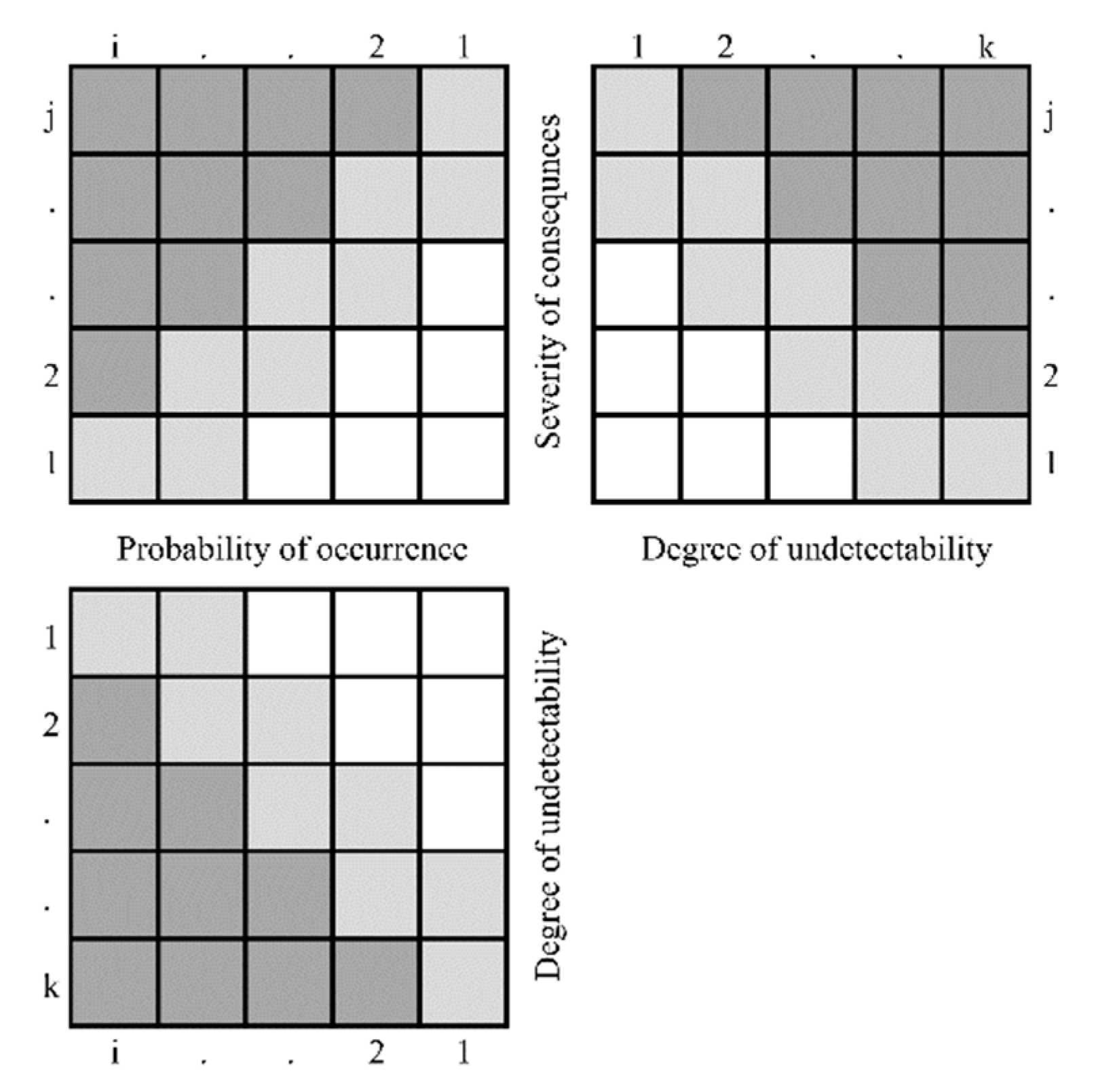
The structure of the PRISM method is a set of three sub-matrices, as visible in Figure 2. Some theoretical priority levels are also visualized as previously modeled in Figure 1.
Based on the scores of the rating factors, a certain incident can be visualized in the Partial Risk Map [13]. If a partial risk is in any of the gray cells in at least one of the three matrices, it will signal the need for control. The location of a partial risk in the map indicates the direction of the action, mitigation, etc., that should be performed.
Although the basic idea of the PRISM methodology has already been described, the deeper analysis of the method cannot be executed without the formal description of the methodology and the definition of aggregation functions for the calculation of the PRISM number. Based on the formal description, the comparison of the RPNs and PRISM numbers determined by different aggregation functions can be executed, the differences can be described, and suggestions can be made for the practical application of the methodology.
2. Materials and Methods
In this section, the focus is on the formal description of different aggregation functions for the PRISM methodology.
The first step is to define incidents and their characteristics. Denote as a failure mode or incident that has three characteristics: o probability of occurrence (occurrence), s severity of consequences (severity), and d degree of undetectability (detection). The characteristics have the following values, , and . For every failure mode or incident, some aggregate risk value can be calculated from the o, s, and d values by applying the ⊗ aggregation function. As mentioned in Section 1, this aggregate value is used to prioritize the incidents, and the higher the aggregated value, the higher the risk of the incident compared to the cases that are assessed with the same aggregation method.
The risk assessment is three dimensional in the case of FMEA, so the RPN value is a point in the three-dimensional space represented by Equation (1).
Denote r(m) = r(o,s,d) = (o⊗s⊗d) a three-dimensional risk evaluation function of m incident in the case of FMEA. For the calculation of the RPN, the typical aggregation method in the industry is the multiplication of o, s, and d values, as shown by Equation (2).
The PRISM methodology observes partial risks that describe three paired characteristics of m incident [13]. Formally, the Partial Risk Map can be described, with a set of three matrices represented by Equations (3)–(5).
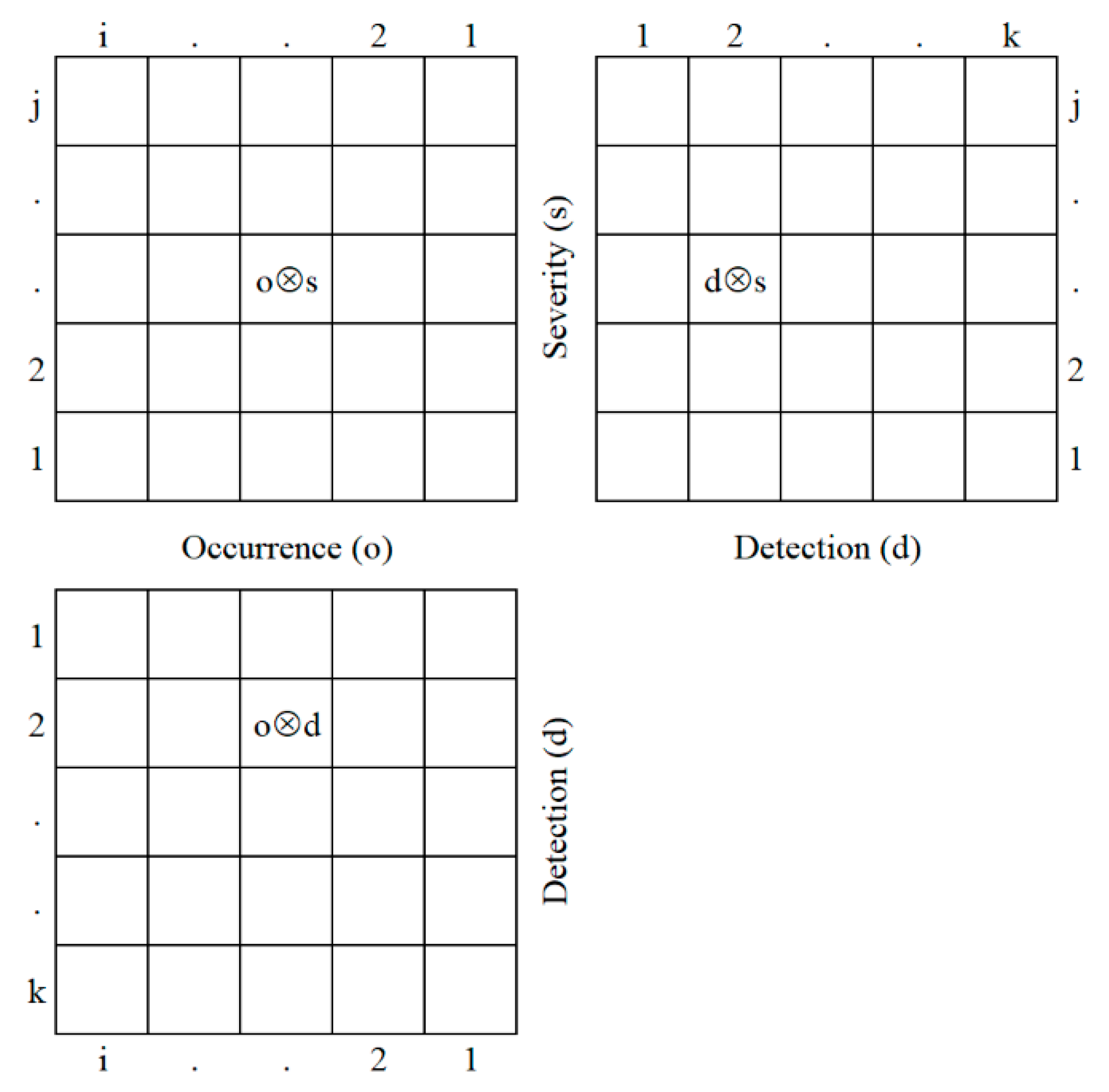
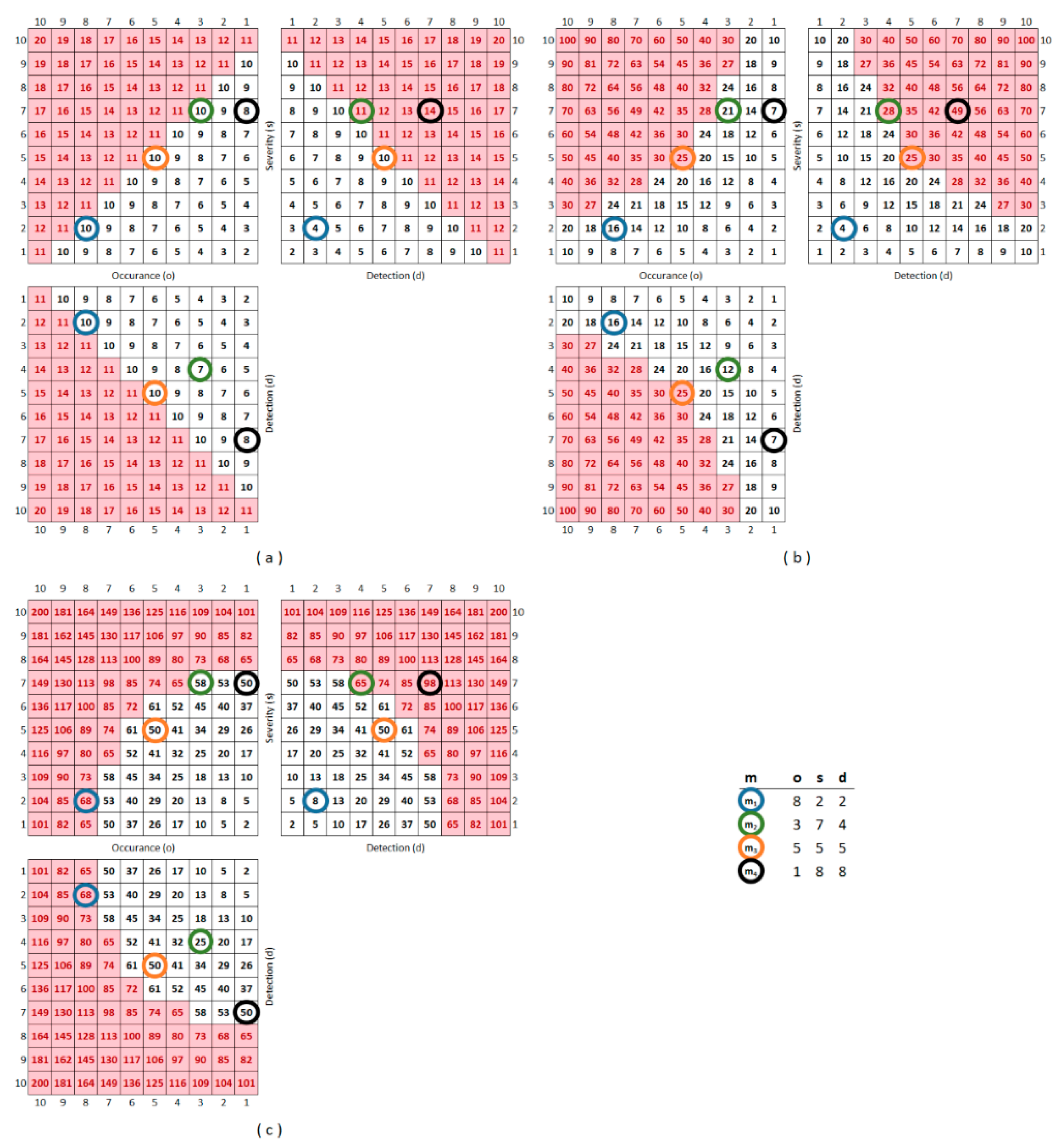
Since the PRISM methodology calculates the aggregate values of the paired characteristics of m incident, denote p(m) = p(o,s,d) = (o⊗s, o⊗d, d⊗s) as the PRISM pattern of an incident. The representation of a theoretical PRISM pattern is visible in Figure 3.
Let M denote the maximal number of m incidents with different risk characteristic combinations, this can be formulated as follows.
In most of the practical cases, , and thus, the value of M is 1000.
The PRISM number of incident m can be given by selecting the maximal value of the three aggregates of p(m). Let PRISM(m) denote the PRISM number of a certain incident. The calculation of the PRISM number is as follows:
In this study, three different formulas are proposed for the PRISM number calculation, as shown by Equations (8)–(10). Note that, the PRISM method is for considering partial risks, no formula is previously given for any calculations.
Let N denote the size of the image set of an aggregation function, i.e., the number of different output values that can be given by an aggregation function. Applying different aggregation functions can result in different N values. In the cases of the applied A(m), M(m), and S(m) aggregation functions, the followings can be given, when , and :
In the case of RPN(m), the following formula can be given, when , and
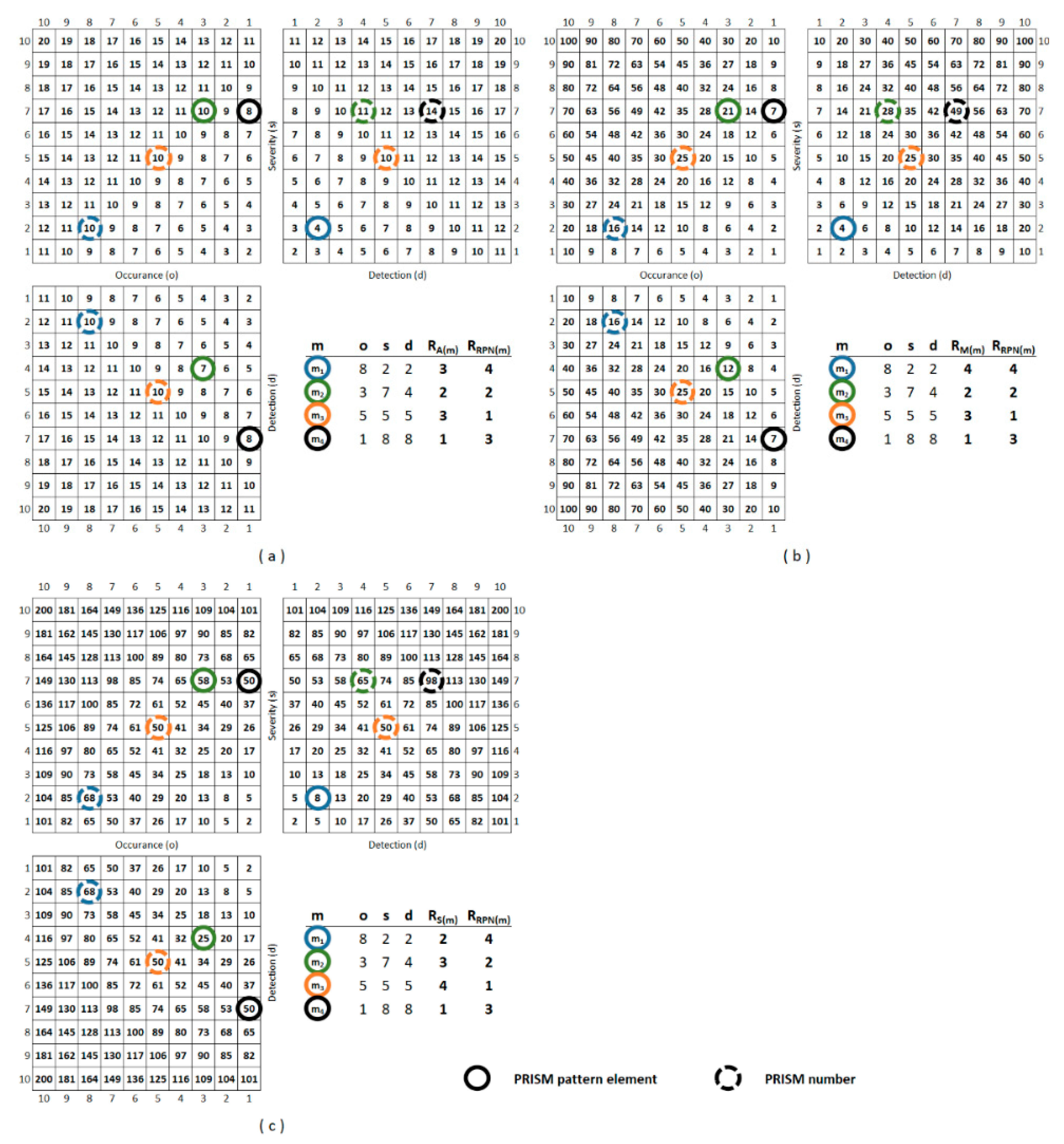
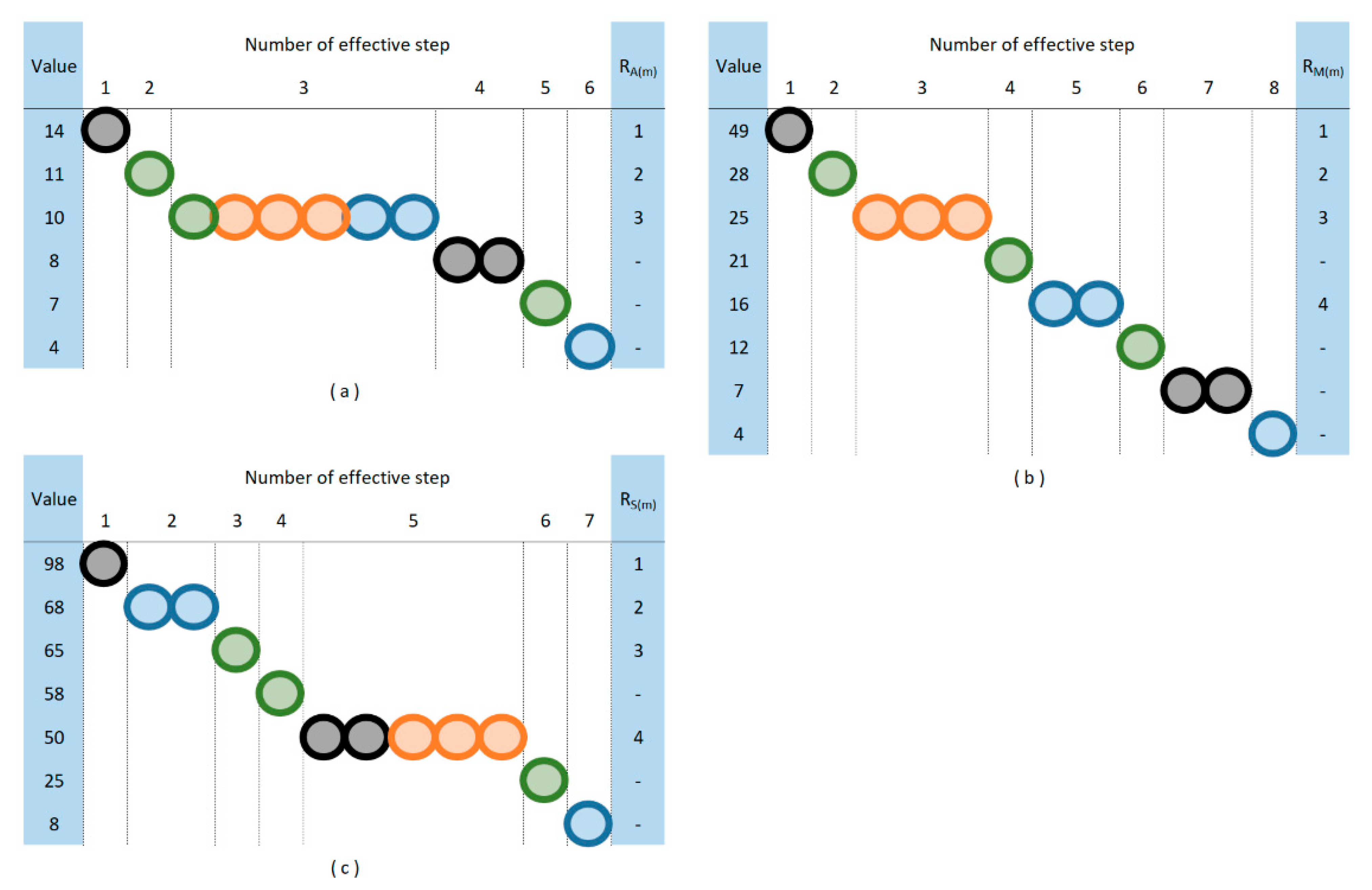
The generated values of the PRISM numbers are visualized in Figure 4 including the PRISM pattern representation of four different (m1, m2, m3, m4) incidents. Based on the PRISM numbers, the ranks of the incidents are also given in Figure 4 as well as the ranks by the RPNs. The higher the value of the PRISM number, the lower the rank. Changing the aggregation function could also change the order of incident priorities as well.
Putting more focus on the application of thresholds, there is an option for further profiling the incident set—instead of only ranking the incidents. As previously described, a threshold is a maximal value of the aggregated result of different m incident patterns that cannot be reached or exceeded by the aggregated result of an incident pattern; otherwise, it signals to the control system. Naturally, the aggregation function of the PRISM number affects also the threshold surface, and the number of steps can be applied from the least strict threshold level to the strictest one (in the case of A(m) from 20 to 2, in the case of M(m) from 100 to 1, and in the case of S(m) from 200 to 2.) The maximum number of different effective threshold levels naturally equals the number of N.
Based on the number N of the aggregation function, the sensitivity for a given threshold can be characterized. Since the A(m) function has the lowest N value, it has sectioning with the largest steps available. In the case of the S(m) function, the N value is the highest, so thresholds can be set by the smallest units. The aggregation function also determines the threshold surface; thus, it affects the set of incidents that need to be treated.
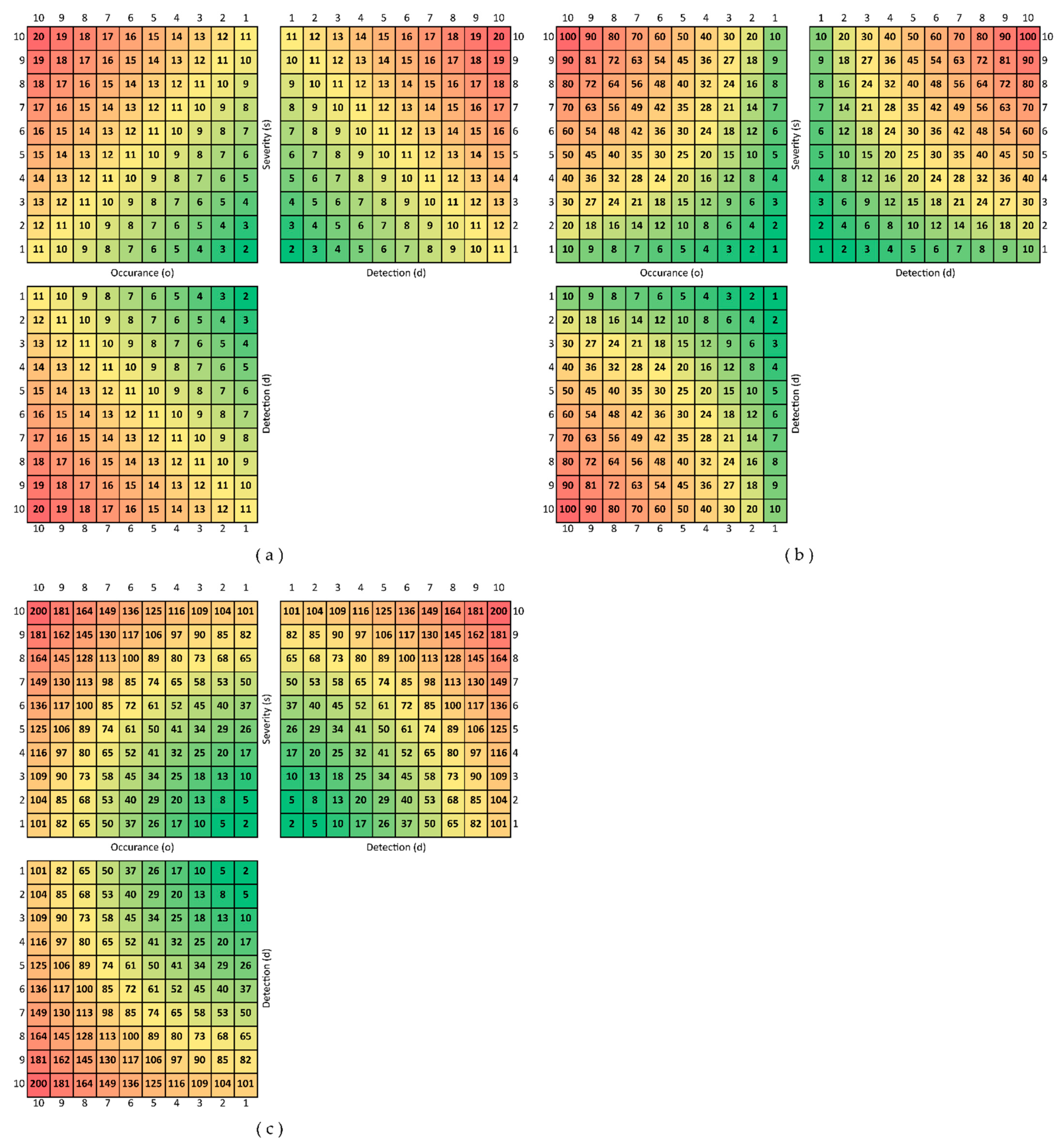
Figure 5 shows an example for the different threshold surfaces in the case of each of the applied aggregation functions. A(m) function results in a linear threshold surface, M(m) results in a convex, and S(m) results in a concave one. In Appendix A, Figure A1 shows the colored partial risk maps, representing all the possible threshold surfaces related to the three aggregation functions.
In Figure 6, the set of m1, m2, m3, and m4 incidents are profiled by applying increasingly stricter threshold levels until all the PRISM pattern elements exceed this threshold.
Of course, the ranking by the PRISM number will not change, but further information on the nature of the risk set can be described as well, which gives a more detailed picture to the decision-makers.
3. Results
In this section, descriptive statistics of the set of PRISM numbers produced by the presented aggregation functions and the set of traditional RPN numbers are described and compared. Some key relations between the aggregation functions of the PRISM method are also presented in this section. Robustness tests of the rankings based on PRISM numbers determined by different aggregation functions are described as well.
3.1. Descriptive Statistics
The descriptive statistics of the three different sets of the PRISM numbers and the set of traditional RPN numbers are shown in Table 1.
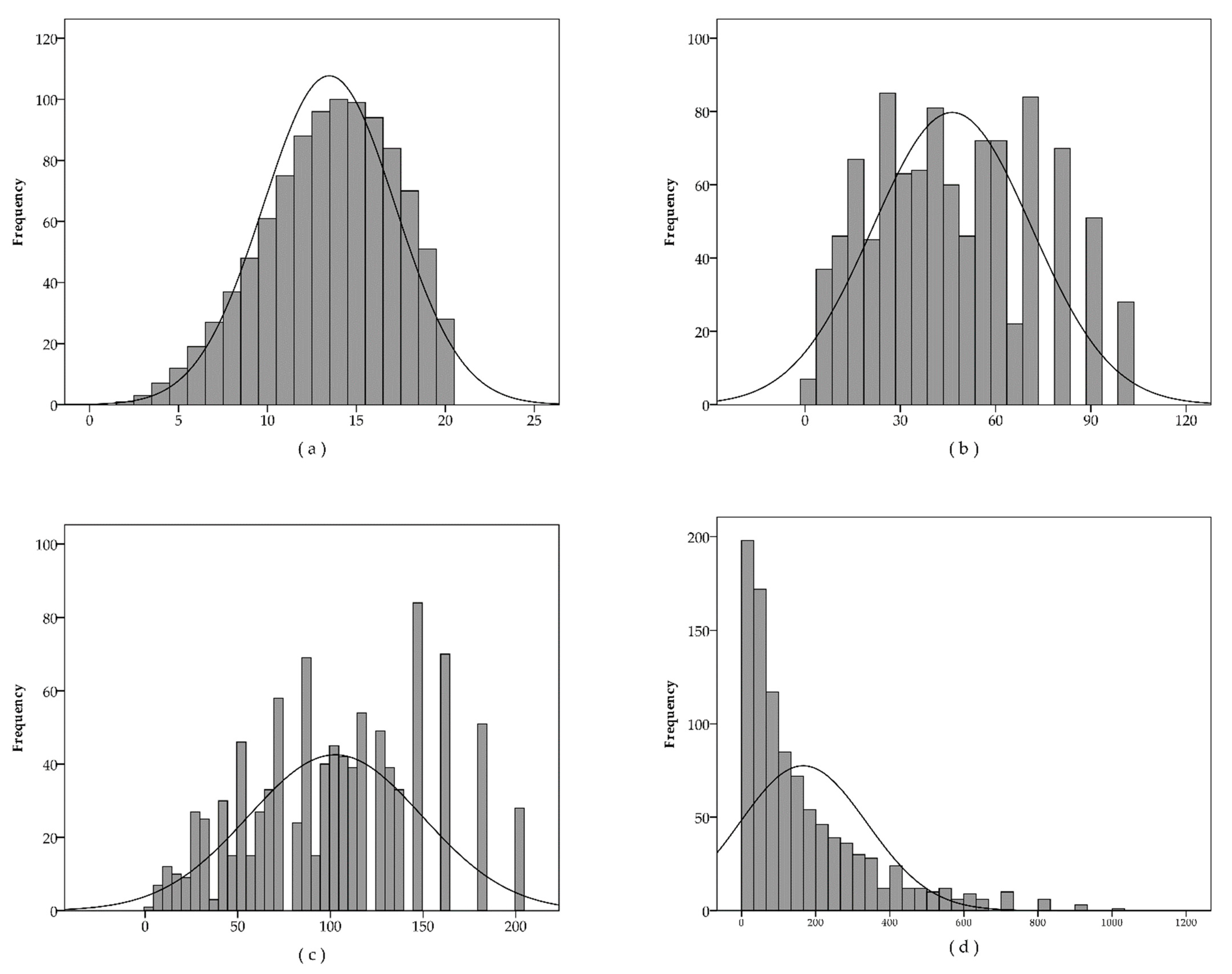
Changing to the PRISM aggregation functions from RPN(m), the number of distinct values (N) drops off from 120 to 19, 42, and 52 for the A(m), M(m), and S(m) versions, respectively, that also decrease the variability of the values. The coefficient of variation (the standard deviation over the mean) is between the quarter and the half of the same value of the traditional RPN. However, the PRISM spreads the values more evenly around the mean, and the absolute values of skewness are also lower than that for the traditional RPN (see Figure 7).
Figure 7 shows that, while the traditional RPN has exponential-like distribution with most of the values close to the lower end of the scale, the PRISM produces more cases on the upper half of its scale.
3.2. Comparison of the Methods
The incidents are ranked by the RPN and the PRISM numbers from the highest to the lowest, ties are resolved by giving the same rank to incidents with the same value—the arithmetic mean of the ranks, i.e., fractional ranking is applied.
All the three PRISM rankings have high (Spearman’s rho) rank correlation to the ranking of traditional RPN, ρ(RRPN(m), RA(m)) = 0.820, ρ(RRPN(m), RM(m)) = 0.842, and ρ(RRPN(m), RS(m)) = 0.778. To evaluate the similarity of the rankings made by the studied methods, the sum of ranking differences (SRD) method [39] is applied. The sum of ranking differences (SRD) [40] method assesses ranking methods according to the sum of the absolute differences in ranks of the objects (i.e., the Manhattan distance) compared to an ideal ranking (a golden standard). If the ideal rank is not known or cannot be explicitly determined, the average rank of the objects can be used since the errors of the different methods cancel each other and the maximum likelihood principle ensures that the most probable ranking is provided by the average [40]. This method is non-parametric and robust, and it is used in several fields of science, see, e.g., [41,42]. In contrast to other statistical methods, such as Spearman’s rho, Kendall’s tau, and Mann–Whitney U test, the SRD not only provides pairwise comparison but also puts all the assessed rankings (aggregation methods) into an order according to their similarity (or dissimilarity) to the golden standard [40]. In this way, SRD also can distinguish groupings and outliers among the ranking methods. Considering all the possible permutations in a ranking, the probability distribution of the SRD values can be determined. This probability distribution is then used to assess the significance of a ranking, i.e., how low is the probability of receiving this ranking as a random permutation.
For the SRD, no universally applicable ranking can be created as a reference in this case because the three characteristics of m are not commensurable with each other, and their relative importance is appraised subjectively. Thus, the average ranking was calculated for each of the 1000 combinations of o, s, and d values. Alongside the traditional RPN and the previously introduced three PRISM aggregations, the total sum (o + s + d), and total squared sum (o2 + s2 + d2) of the three characteristics were used as a rank determining method. This was necessary to avoid the bias toward the three new PRISM-based approaches (similar to each other) against the singleton of the traditional RPN. This setting has equal number of approaches for the pairwise holistic comparison and also for each aggregation. The normalized SRD distances from this reference are shown in Table 2. For the normalization, the theoretical maximum of SRD was calculated and it received the value 1 on the scale. Considering all the possible permutations of the M = 1000 cases, the normalized SRD values can be described with a normal distribution with 0.6667 mean and 0.0133 standard deviation.
The average ranking of the three PRISM aggregations is used as a reference when only these functions are compared to each other. The SRD of the three methods to this reference is shown in the diagonal of Table 3. The upper triangle of the table gives the pairwise distance of the methods. From the results, it can be inferred that the additive PRISM gives the closest ranking to the average, and it is at an equal distance from the other two methods. The Spearman rho coefficients are in the lower triangle and indicate high rank correlations between the rankings.
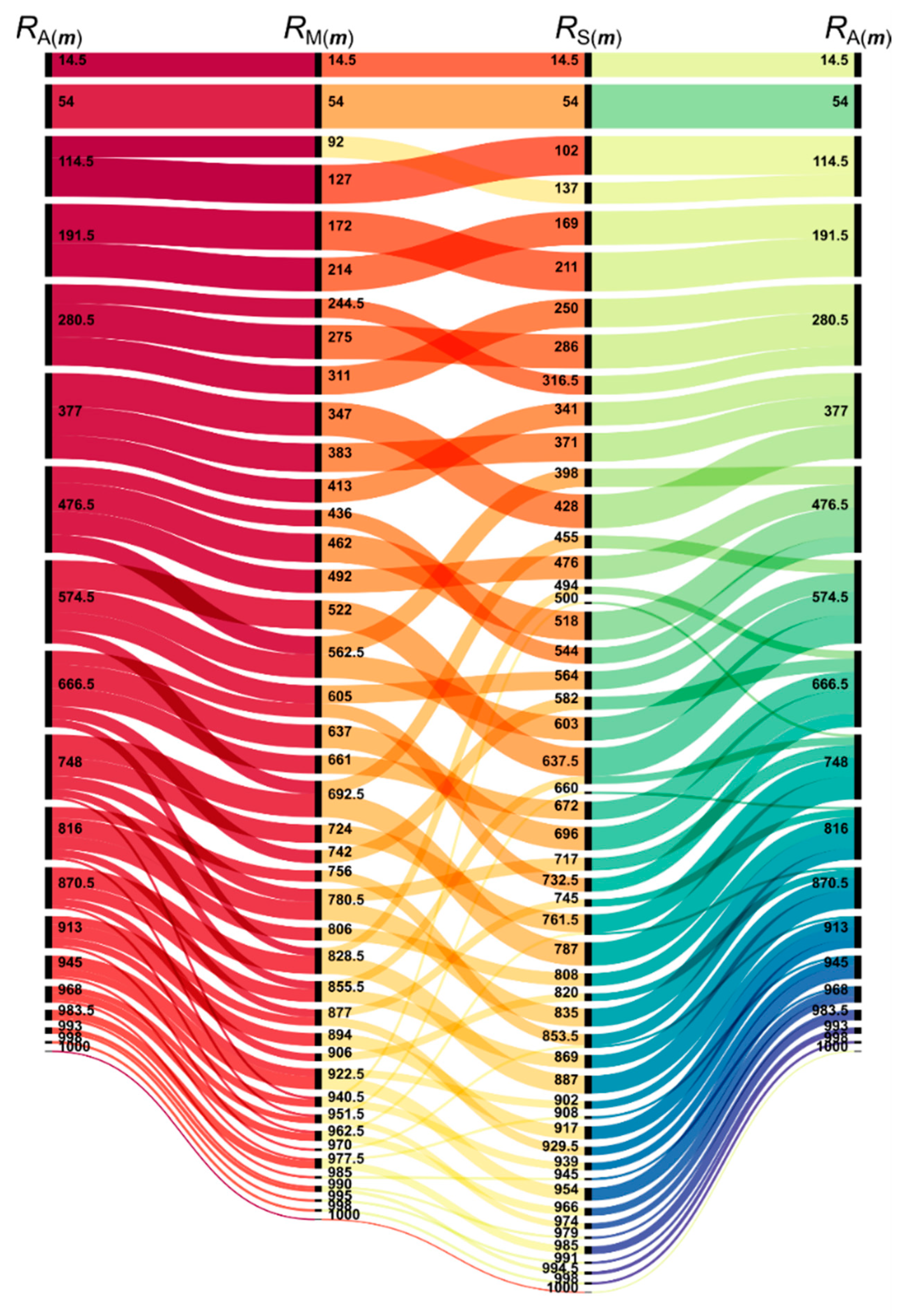
The method-by-method change in ranking or classification can also be visualized with alluvial diagrams (Figure 8).
The three algorithms rank the most important 79 (28 + 51) cases from the 1000 in the same way (see Figure 8). After that, there are some rearrangements in the rankings. The addition and the multiplication have almost the same order in the first half of the possible 1000 cases, multiplication just breaks the ties of the addition; however, the multiplication ranks further back some cases in the second half of the cases. The sum of squares produces a very different order and breaks the ties of the addition in the opposite order than the multiplication does immediately after the first 79 cases.
Let denote RA(m), RM(m), and RS(m) denote the ranks of m incident according to the value produced by A(m), M(m), and S(m) aggregation or evaluation functions, respectively. The rank here means an order of importance and means that incident m is more important than incident l, and incident k has the same importance as l.
In Figure 8, several groups can be identified in which the methods give different priority orders, for instance, see Equations (15)–(17).
Evidently, any permutation of the scores of m produces the same output value, and thus, the same rank for the given evaluation function. The points in Equation (17) are on three perpendicular frontiers of A(m) that are between the concave and convex frontiers of S(m) and M(m) as the SRD values also indicated in Table 2.
3.3. Effect of the Scale
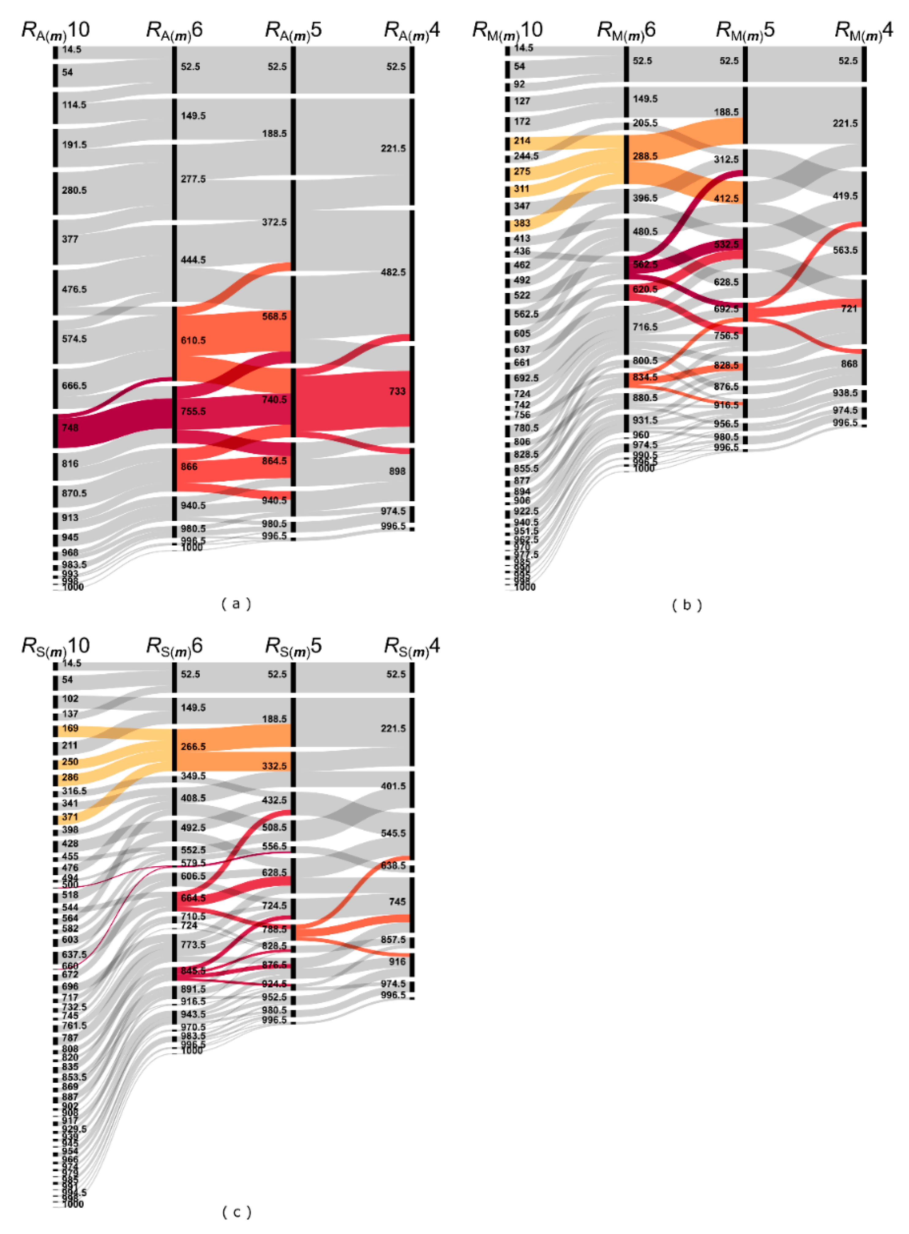
The ranking can vary not only when the evaluation method is altered but also with the change of resolution of characteristics of the incidents while the same evaluation method is maintained. If the resolution of the scale that is used for the specification of the o, s, and d values decreases from range 10 (RA(m)10, RM(m)10, and RS(m)10) to 6 (RA(m)6, RM(m)6, and RS(m)6), 5 (RA(m)5, RM(m)5, and RS(m)5), or 4 (RA(m)4, RM(m)4, and RS(m)4), the rank of the incidents can change even within the same evaluation method. However, according to the Spearman’s rank correlations (see Table 4), the rankings can maintain most of their priority order even with a rougher scale, the correlation coefficient between the original and any investigated lower-resolution scale with the same aggregation is not lower than 0.938. The correlation is even higher if one switches between methods but keeps the same scale of the risk factor scores (o, s, and d); see the shaded cells in Table 4. Comparing the SRD values in the Table 2 and Table 4, it can be seen that even using PRISM with fewer steps results in a lower distance from the golden standard than the cumulative Manhattan distance of the RPN (0.2073).
Figure 9 shows the rankings in the case of range 10 (RA(m)10, RM(m)10 and RS(m)10), 6 (RA(m)6, RM(m)6 and RS(m)6), 5 (RA(m)5, RM(m)5 and RS(m)5), and 4 (RA(m)4, RM(m)4 and RS(m)4) of the methods, and whether or how they change on transferring from one to the another. The most robust ranking is made by A(m); here, just a few swaps happen between neighboring categories. In the case of the other aggregation methods (M(m) and S(m)), the lower resolution makes the incident skip categories in both directions, which alters the priority order considerably. The higher the number of crossings on the alluvial diagrams (Figure 9), the lower is the correlation between the rankings (Table 4).
4. Discussion
The PRISM method is effective in identifying risks, where there is a high partial risk; however, the entire risk level does not make any signal for the control system. In the cases of high partial risks, the possibility of sudden failures can be higher, which can lead to unexpected costs, loss of availability, unplanned breakdowns, unnecessary environmental impacts, etc. Similar to the FMEA methodology, the PRISM method also gives high priority to those incidents, where all the factor values (o, s, d) are relatively high, but PRISM puts also more focus on those cases where only two of the factor values are relatively high while the third one is relatively low [13]. In these cases, a relatively small increase in the value of the third factor can result in a significant increase in the entire risk level.
Applying different aggregation functions for the calculation of the PRISM number generates different partial risk maps, with different properties. Instead of conventional FMEA, which applies multiplication [43] for aggregating the three factors, PRISM creates the opportunity of application in scenarios related to the risk assessment process.
In the case of the S(m) function (sum of squares), an additional focus exists besides the attention to partial risks. Since the S(m) function provides a concave threshold surface, the additional focus is on the higher priority of those incidents, which have a very high value at one factor. An example for this case is m1 in Figure 5. Applying the S(m) function, the relative priority of m1 significantly increases; however, when applying other functions for creating the PRISM number, this incident stays in the background.
This function can be proposed for practical cases, where signaling of very high values of any factor is important. Since a new trend is unfolding in the automotive industry, special attention is given to the severity factor in the new AIAG-VDA FMEA handbook [44]. The S(m) PRISM function can be useful in a risk assessment environment where the focus is on high-priority incidents that have high severity values. The S(m) function is also offered for testing, modification, and development in safety-related cases as well, such as in the energy industry [45], healthcare industry [46], or in the field of compliance management [47].
In the case of the M(m) function (multiplication), the focus is on the “mid-values” since this function provides a convex surface (see Figure A1). The outputs of the M(m) function have the highest correlation to the RPN(m) outputs. Thus, the application of M(m) can be offered in cases where the application experience of RPN is high, but the possible effects of the partial risks should be useful to be considered. For assessing compliance risks, multiplication is applied for constructing the risk matrix [17], but the results cannot be as detailed as applying the M(m) function of the PRISM method.
As is clearly visible in the results, the A(m) function stays between the previously discussed two functions. Based on the normalized SRD values (see Table 3), the A(m) function is almost definitely in the center between the M(m) and S(m) functions. This can be visually proved by Figure 8 since there are significantly more changes in the rankings between the M(m) and S(m) functions than between the A(m) and M(m) or the A(m) and S(m) ones. Although an addition function is already applied for creating a risk matrix of o and s [7], the analysis could be more detailed by applying the A(m) function of PRISM.
The priority order provided by the PRISM method is robust to the resolution of the scales of the risk factors o, s, and d. If the number of distinct categories decreases from the conventional 10 to a reasonable low value, the PRISM keeps a high rate of the original order. This also means that it is applicable for fuzzy approaches, since in fuzzification, reducing the number of categories of the crisp set to the fuzzy set with help of the membership function is the same as coherently using broader risk factor categories (in Table 4 and Figure 9).
Applying any of the PRISM functions, the nature of the incident risk can be described more precisely than in the case of [30], where only the RPN function is applied. According to [13,37], the combined application of the traditional RPN and PRISM number can result in a balanced risk assessment since the effects of partial risks and risk priority number can be adjusted using any of the PRISM functions.
When more incidents have the same PRISM number, the one that has its value in more submatrices should be prioritized. As a management tool, the PRISM methodology gives a better option than traditional RM [17] or FMEA [30] in visualizing the risk assessment results, and the estimated outcomes after risk reduction actions were executed were more favorable.
Although applying PRISM functions can improve the usability of the partial risk map methodology [13], other potentials of the method can be developed in future works. Based on many lessons learned related to other previously created platform risk assessment methods (FMEA, RM, FTA, HAZOP, etc.), possible development directions of the PRISM method can be forecasted. Since the most methodological similarity can be identified between PRISM and FMEA, based on some systematic and rigorous literature reviews of FMEA developments [28,48,49], some developmental fields can be highlighted for the PRISM method as well.
Although many criticisms expressed that different combinations of o, s, and d can result in the same RPN while the hidden risk content behind the RPN is different [21,22,23,24,25,47,50,51], the PRISM method solves this problem, since it describes hidden risks with different aggregation functions and visualizes hidden risks via the PRISM pattern. On the other hand, realizing more potentials for the methodology, one development direction can be of the future of applying MCDM methods such as AHP [1,52] or ANP [32] or multilevel methods such as TREF [53] for solving the possible subjective ranking issues of the evaluators. Another major direction in the future can be to describe the nature and applicability of different partial risk maps using different aggregation functions in different submatrices of the map.
5. Conclusions
Risk assessment and mitigation is an evergreen topic among practitioners and scholars. One of the most widespread tools to evaluate and prioritize risky incidents is FMEA, which condenses several risk factors into one variable, the RPN. However, this simple condensing operation neglects a lot of information about the investigated incidents. Several methods try to enhance this risk evaluation and prioritization process by balancing between the information loss and handling a multicriteria decision-making problem.
The PRISM method and some of its possible aggregation functions are studied in this paper to describe how it relates to the traditional FMEA and which properties of the PRISM method and its functions make it suitable for risk evaluation and prioritization in different cases. The PRISM method can focus the user’s attention to such incidents where just some of the risk factors are high and the RPN of the traditional FMEA falls below the stimulus threshold of the process but a small change in the lower value factor(s) would launch up the aggregated value. Choosing the appropriate aggregation method can fine-tune this feature of the PRISM, increasing (S(m)) or decreasing (M(m)) its sensitivity toward these kinds of incidents.
Though the PRISM can reveal some hidden potential risks, it cannot tell how one can eliminate or mitigate these risks, the PRISM is just a risk assessment method and not a risk management tool. Thus, it cannot decide for the user where (on what level) the threshold should be drawn, but the priority order given by the PRISM and resource constraints can specify a set of incidents to be treated.
As a limitation of the PRISM, it can be stated that its capability depends on the exactitude of its inputs: although the uncertainty or fuzziness in the determination risk factor values does not radically change the priority order of the incidents, a biased evaluation of o, s, or d can turn the focus of risk management to a wrong direction. The effects of biased risk factor evaluation or using weights for these factors in the aggregation is a possible topic of future research.
Author Contributions
Conceptualization, methodology, formal analysis, visualization, writing—original draft preparation, and writing—review and editing, F.B. and C.H. All authors have read and agreed to the published version of the manuscript.
Funding
The work was supported by the TKP2020-NKA-10 project financed under the 2020-4.1.1-TKP2020 Thematic Excellence Program by the National Research, Development, and Innovation Fund of Hungary.
Data Availability Statement
Not applicable.
Conflicts of Interest
The authors declare no conflict of interest.
Appendix A
Figure A1.
Colored visualization of the possible thresholds of the partial risk maps. (a) The threshold surfaces in the case of A(m), (b) threshold surfaces in the case of M(m), and (c) threshold surfaces in the case of S(m).
Figure A1.
Colored visualization of the possible thresholds of the partial risk maps. (a) The threshold surfaces in the case of A(m), (b) threshold surfaces in the case of M(m), and (c) threshold surfaces in the case of S(m).

References
- Braglia, M. MAFMA: Multi-attribute failure mode analysis. Int. J. Qual. Reliab. Manag. 2000, 17, 1017–1033. [Google Scholar] [CrossRef] [Green Version]
- Shan, H.; Tong, Q.; Shi, J.; Zhang, Q. Risk Assessment of Express Delivery Service Failures in China: An Improved Failure Mode and Effects Analysis Approach. J. Theor. Appl. Electron. Commer. Res. 2021, 16, 2490–2514. [Google Scholar] [CrossRef]
- Somi, S.; Seresht, N.G.; Fayek, A.R. Developing a risk breakdown matrix for onshore wind farm projects using fuzzy case-based reasoning. J. Clean. Prod. 2021, 311, 127572. [Google Scholar] [CrossRef]
- Marhavilas, P.K.; Filippidis, M.; Koulinas, G.K.; Koulouriotis, D.E. Safety-assessment by hybridizing the MCDM/AHP & HAZOP-DMRA techniques through safety’s level colored maps: Implementation in a petrochemical industry. Alex. Eng. J. 2022, 61, 6959–6977. [Google Scholar] [CrossRef]
- Zhang, J.; Kang, J.; Sun, L.; Bai, X. Risk assessment of floating offshore wind turbines based on fuzzy fault tree analysis. Ocean Eng. 2021, 239, 109859. [Google Scholar] [CrossRef]
- Shafiee, M.; Enjema, E.; Kolios, A. An Integrated FTA-FMEA Model for Risk Analysis of Engineering Systems: A Case Study of Subsea Blowout Preventers. Appl. Sci. 2019, 9, 1192. [Google Scholar] [CrossRef] [Green Version]
- Schafer, H.L.; Beier, N.A.; Macciotta, R. A Failure Modes and Effects Analysis Framework for Assessing Geotechnical Risks of Tailings Dam Closure. Minerals 2021, 11, 1234. [Google Scholar] [CrossRef]
- Bradley, J.R.; Guerrero, H.H. An Alternative FMEA Method for Simple and Accurate Ranking of Failure Modes. Decis. Sci. 2011, 42, 743–771. [Google Scholar] [CrossRef]
- Kang, J.; Sun, L.; Sun, H.; Wu, C. Risk assessment of floating offshore wind turbine based on correlation-FMEA. Ocean Eng. 2017, 129, 382–388. [Google Scholar] [CrossRef]
- Ivančan, J.; Lisjak, D. New FMEA Risks Ranking Approach Utilizing Four Fuzzy Logic Systems. Machines 2021, 9, 292. [Google Scholar] [CrossRef]
- Fabis-Domagala, J.; Domagala, M.; Momeni, H. A Concept of Risk Prioritization in FMEA Analysis for Fluid Power Systems. Energies 2021, 14, 6482. [Google Scholar] [CrossRef]
- Carnero, M.C. Waste Segregation FMEA Model Integrating Intuitionistic Fuzzy Set and the PAPRIKA Method. Mathematics 2020, 8, 1375. [Google Scholar] [CrossRef]
- Bognár, F.; Benedek, P. A Novel Risk Assessment Methodology—A Case Study of the PRISM Methodology in a Compliance Management Sensitive Sector. Acta Polytech. Hung. 2021, 18, 89–108. [Google Scholar] [CrossRef]
- Bognár, F.; Benedek, P. Case Study on a Potential Application of Failure Mode and Effects Analysis in Assessing Compliance Risks. Risks 2021, 9, 164. [Google Scholar] [CrossRef]
- Qazi, A.; Shamayleh, A.; El-Sayegh, S.; Formaneck, S. Prioritizing risks in sustainable construction projects using a risk matrix-based Monte Carlo Simulation approach. Sustain. Cities Soc. 2021, 65, 102576. [Google Scholar] [CrossRef]
- Wang, R.; Wang, J. Risk Analysis of Out-drum Mixing Cement Solidification by HAZOP and Risk Matrix. Ann. Nucl. Energy 2020, 147, 107679. [Google Scholar] [CrossRef]
- Losiewicz-Dniestrzanska, E. Monitoring of compliance risk in the bank. Procedia Econ. Financ. 2015, 26, 800–805. [Google Scholar] [CrossRef] [Green Version]
- Jeon, H.; Park, K.; Kim, J. Comparison and Verification of Reliability Assessment Techniques for Fuel Cell-Based Hybrid Power System for Ships. J. Mar. Sci. Eng. 2020, 8, 74. [Google Scholar] [CrossRef] [Green Version]
- Zheng, H.; Tang, Y. Deng Entropy Weighted Risk Priority Number Model for Failure Mode and Effects Analysis. Entropy 2020, 22, 280. [Google Scholar] [CrossRef] [Green Version]
- Lv, Y.; Liu, Y.; Jing, W.; Woźniak, M.; Damaševičius, R.; Scherer, R.; Wei, W. Quality Control of the Continuous Hot Pressing Process of Medium Density Fiberboard Using Fuzzy Failure Mode and Effects Analysis. Appl. Sci. 2020, 10, 4627. [Google Scholar] [CrossRef]
- Lo, H.W.; Liou, J.J.H.; Huang, C.N.; Chuang, Y.C. A novel failure mode and effect analysis model for machine tool risk analysis. Reliab. Eng. Syst. Saf. 2019, 183, 173–183. [Google Scholar] [CrossRef]
- Liou, J.J.H.; Liu, P.C.Y.; Lo, H.W. A Failure Mode Assessment Model Based on Neutrosophic Logic for Switched-Mode Power Supply Risk Analysis. Mathematics 2020, 8, 2145. [Google Scholar] [CrossRef]
- Chang, T.W.; Lo, H.W.; Chen, K.Y.; Liou, J.J.H. A Novel FMEA Model Based on Rough BWM and Rough TOPSIS-AL for Risk Assessment. Mathematics 2019, 7, 874. [Google Scholar] [CrossRef] [Green Version]
- Lo, H.W.; Liou, J.J.H. A novel multiple-criteria decision-making-based FMEA model for risk assessment. Appl. Soft Comput. 2018, 73, 684–696. [Google Scholar] [CrossRef]
- Ghoushchi, S.J.; Yousefi, S.; Khazaeili, M. An extended FMEA approach based on the Z-MOORA and fuzzy BWM for prioritization of failures. Appl. Soft Comput. 2019, 81, 105505. [Google Scholar] [CrossRef]
- Chanamool, N.; Naenna, T. Fuzzy FMEA application to improve decision-making process in an emergency department. Appl. Soft Comput. 2016, 43, 441–453. [Google Scholar] [CrossRef]
- Liu, H.C.; Liu, L.; Liu, N.; Mao, X.L. Risk evaluation in failure mode and effects analysis with extended VIKOR method under fuzzy environment. Expert Syst. Appl. 2012, 39, 12926–12934. [Google Scholar] [CrossRef]
- Liu, H.C.; Liu, L.; Liu, N. Risk evaluation approaches in failure mode and effects analysis: A literature review. Expert Syst. Appl. 2013, 40, 828–838. [Google Scholar] [CrossRef]
- Kutlu, A.C.; Ekmekçioğlu, M. Fuzzy failure modes and effects analysis by using fuzzy TOPSIS-based fuzzy AHP. Expert Syst. Appl. 2012, 39, 61–67. [Google Scholar] [CrossRef]
- Zúñiga, A.A.; Baleia, A.; Fernandes, J.; Branco, P.J.D.C. Classical Failure Modes and Effects Analysis in the Context of Smart Grid Cyber-Physical Systems. Energies 2020, 13, 1215. [Google Scholar] [CrossRef] [Green Version]
- Sharma, R.K.; Kumar, D.; Kumar, P. Modeling and analysing system failure behaviour using RCA, FMEA and NHPPP models. Int. J. Qual. Reliab. Manag. 2007, 24, 525–546. [Google Scholar] [CrossRef]
- Zammori, F.; Gabbrielli, R. ANP/RPN: A multi criteria evaluation of the risk priority number. Qual. Reliab. Eng. Int. 2011, 28, 85–104. [Google Scholar] [CrossRef]
- Gargama, H.; Chaturvedi, S.K. Criticality assessment models for failure mode effects and criticality analysis using fuzzy logic. IEEE Trans. Reliab. 2011, 60, 102–110. [Google Scholar] [CrossRef]
- Braglia, M.; Frosolini, M.; Montanari, R. Fuzzy criticality assessment model for failure modes and effects analysis. Int. J. Qual. Reliab. Manag. 2003, 20, 503–524. [Google Scholar] [CrossRef]
- Seyed-Hosseini, S.M.; Safaei, N.; Asgharpour, M.J. Reprioritization of failures in a system failure mode and effects analysis by decision making trial and evaluation laboratory technique. Reliab. Eng. Syst. Saf. 2006, 91, 872–881. [Google Scholar] [CrossRef]
- Abdelgawad, M.; Fayek, A.R. Risk management in the construction industry using combined fuzzy FMEA and fuzzy AHP. J. Constr. Eng. Manag. 2010, 136, 1028–1036. [Google Scholar] [CrossRef]
- Forgács, A.; Lukács, J.; Horváth, R. The Investigation of the Applicability of Fuzzy Rule-based Systems to Predict Economic Decision-Making. Acta Polytech. Hung. 2021, 18, 97–115. [Google Scholar] [CrossRef]
- Rosenberger, P.; Tick, J. Multivariate Optimization of PMBOK, Version 6 Project Process Relevance. Acta Polytech. Hung. 2021, 18, 9–28. [Google Scholar] [CrossRef]
- Kollár-Hunek, K.; Héberger, K. Method and model comparison by sum of ranking differences in cases of repeated observations (ties). Chemom. Intell. Lab. Syst. 2013, 127, 139–146. [Google Scholar] [CrossRef]
- Héberger, K.; Kollár-Hunek, K. Sum of ranking differences for method discrimination and its validation: Comparison of ranks with random numbers. J. Chemom. 2011, 25, 151–158. [Google Scholar] [CrossRef]
- Ipkovich, Á.; Héberger, K.; Abonyi, J. Comprehensible Visualization of Multidimensional Data: Sum of Ranking Differences-Based Parallel Coordinates. Mathematics 2021, 9, 3203. [Google Scholar] [CrossRef]
- Mizik, T.; Gál, P.; Török, Á. Does Agricultural Trade Competitiveness Matter? The Case of the CIS Countries. AGRIS On-Line Pap. Econ. Inform. 2020, 12, 61–72. [Google Scholar] [CrossRef] [Green Version]
- Wang, Q.; Jia, G.; Jia, Y.; Song, W. A new approach for risk assessment of failure modes considering risk interaction and propagation effects. Reliab. Eng. Syst. Saf. 2021, 216, 108044. [Google Scholar] [CrossRef]
- AIAG; VDA. FMEA Handbook, 1st ed.; Automotive Industry Action Group: Southfield, MI, USA, 2019. [Google Scholar]
- Koval, K.; Torabi, M. Failure mode and reliability study for Electrical Facility of the High Temperature Engineering Test Reactor. Reliab. Eng. Syst. Saf. 2021, 210, 107529. [Google Scholar] [CrossRef]
- Abrahamsen, A.B.; Abrahamsen, E.B.; Høyland, S. On the need for revising healthcare failure mode and effect analysis for assessing potential for patient harm in healthcare processes. Reliab. Eng. Syst. Saf. 2016, 155, 160–168. [Google Scholar] [CrossRef]
- Benedek, P. Compliance management—A new response to legal and business challenges. Acta Polytech. Hung. 2012, 9, 135–148. [Google Scholar]
- Liu, H.C.; Chen, X.Q.; Duan, C.Q.; Wang, Y.M. Failure mode and effect analysis using multi-criteria decision making methods: A systematic literature review. Comput. Ind. Eng. 2019, 135, 881–897. [Google Scholar] [CrossRef]
- Huang, J.; You, J.X.; Liu, H.C.; Song, M.S. Failure mode and effect analysis improvement: A systematic literature review and future research agenda. Reliab. Eng. Syst. Saf. 2020, 199, 106885. [Google Scholar] [CrossRef]
- Tay, K.M.; Lim, C.P. Enhancing the failure mode and effect analysis methodology with fuzzy inference techniques. J. Intell. Fuzzy Syst. 2010, 21, 135–146. [Google Scholar] [CrossRef]
- Zhang, Z.F.; Chu, X.N. Risk prioritization in failure mode and effects analysis under uncertainty. Expert Syst. Appl. 2011, 38, 206–214. [Google Scholar] [CrossRef]
- Ilangkumaran, M.; Shanmugam, P.; Sakthivel, G.; Visagavel, K. Failure mode and effect analysis using fuzzy analytic hierarchy process. Int. J. Product. Qual. Manag. 2014, 14, 296–313. [Google Scholar] [CrossRef]
- Kosztyán, Z.T.; Csizmadia, T.; Kovács, Z.; Mihálcz, I. Total Risk Evaluation Framework. Int. J. Qual. Reliab. Manag. 2020, 37, 575–608. [Google Scholar] [CrossRef]
Figure 1.
Visualization example of the risk matrix.

Figure 2.
Visualization example of the partial risk map.

Figure 3.
The visualization of the PRISM pattern in the partial risk map.

Figure 4.
The visualization of the PRISM patterns and PRISM numbers in the case of A(m), M(m), and S(m) functions. Picture part (a) shows all the results of p(m) and PRISM(m) in the case of A(m), part (b) represents the results for M(m), while part (c) shows the results for S(m).
Figure 4.
The visualization of the PRISM patterns and PRISM numbers in the case of A(m), M(m), and S(m) functions. Picture part (a) shows all the results of p(m) and PRISM(m) in the case of A(m), part (b) represents the results for M(m), while part (c) shows the results for S(m).

Figure 5.
The example thresholds are set at the 25th percentiles of all the incidents. (a) The threshold surface in the case of A(m), (b) the threshold surface in the case of M(m), and (c) the threshold surface in the case of S(m).
Figure 5.
The example thresholds are set at the 25th percentiles of all the incidents. (a) The threshold surface in the case of A(m), (b) the threshold surface in the case of M(m), and (c) the threshold surface in the case of S(m).

Figure 6.
(a) The profile of the incident set in the case of A(m), (b) the case of M(m), and (c) the case of S(m).
Figure 6.
(a) The profile of the incident set in the case of A(m), (b) the case of M(m), and (c) the case of S(m).

Figure 7.
The histograms of all the possible results of the assessment algorithms, when o, s, and d ∈ [1,2,…,10]. Picture part (a) shows the histogram of A(m), part (b) shows the histogram of M(m), part (c) shows the histogram of S(m) while part (d) shows the histogram of RPN(m).
Figure 7.
The histograms of all the possible results of the assessment algorithms, when o, s, and d ∈ [1,2,…,10]. Picture part (a) shows the histogram of A(m), part (b) shows the histogram of M(m), part (c) shows the histogram of S(m) while part (d) shows the histogram of RPN(m).

Figure 8.
The alluvial diagram of the rankings of the three PRISM methods. One node represents the incidents with the same fractional rank (the value on the node).
Figure 8.
The alluvial diagram of the rankings of the three PRISM methods. One node represents the incidents with the same fractional rank (the value on the node).

Figure 9.
The alluvial diagram of the rankings of the three PRISM methods—addition (a), multiplication (b), and the sum of squares (c)—when the range of the scores (o, s, d) decreases from 10 to 6, 5, and 4. Some cases are colored to make them more distinguishable.
Figure 9.
The alluvial diagram of the rankings of the three PRISM methods—addition (a), multiplication (b), and the sum of squares (c)—when the range of the scores (o, s, d) decreases from 10 to 6, 5, and 4. Some cases are colored to make them more distinguishable.


Table 1.
Descriptive statistics related to the different PRISM numbers and the traditional RPN number.
Table 1.
Descriptive statistics related to the different PRISM numbers and the traditional RPN number.
| A(m) | M(m) | S(m) | RPN(m) | ||
|---|---|---|---|---|---|
| Number of incidents (M) | 1000 | 1000 | 1000 | 1000 | |
| Mean | 13.48 | 46.32 | 102.64 | 166.38 | |
| Std. error of mean | 0.117 | 0.791 | 1.483 | 5.424 | |
| Mode | 14 | 90 | 181 | 60 | |
| Std. deviation | 3.704 | 25.012 | 46.901 | 171.509 | |
| Variance | 13.721 | 625.594 | 2199.668 | 29,415.400 | |
| Coefficient of variation | 0.275 | 0.540 | 0.457 | 1.031 | |
| Skewness | −0.383 | 0.274 | 0.044 | 1.672 | |
| Kurtosis | −0.398 | −0.838 | −0.727 | 2.828 | |
| Number of different ranks (N) | 19 | 42 | 52 | 120 | |
| Range | 18 | 99 | 198 | 999 | |
| Minimum | 2 | 1 | 2 | 1 | |
| Maximum | 20 | 100 | 200 | 1000 | |
| Percentiles | 25 | 11.00 | 25.00 | 65.00 | 42.00 |
| 50 | 14.00 | 45.00 | 101.00 | 105.00 | |
| 75 | 16.00 | 64.00 | 136.00 | 240.00 | |
Table 2.
Sum of ranking differences compared to the average rankings.
| Method | Formula | SRD |
|---|---|---|
| RPN(m) | 0.2074 | |
| A(m) | 0.0653 | |
| M(m) | 0.0897 | |
| S(m) | 0.0967 |
Table 3.
Sum of ranking differences (SRD) between each PRISM aggregation pair in the upper triangle, SRD compared to the average of PRISM rankings in the diagonal, Spearman’s rho values in the lower triangle.
Table 3.
Sum of ranking differences (SRD) between each PRISM aggregation pair in the upper triangle, SRD compared to the average of PRISM rankings in the diagonal, Spearman’s rho values in the lower triangle.
| A(m) Ranking | M(m) Ranking | S(m) Ranking | |
|---|---|---|---|
| A(m) ranking | SRDA = 0.0170 | SRDAM = 0.0594 | SRDAS = 0.0596 |
| M(m) ranking | ρMA = 0.990 | SRDM = 0.0606 | SRDMS = 0.1182 |
| S(m) ranking | ρSA = 0.988 | ρSM = 0.957 | SRDS = 0.0624 |
Table 4.
Spearman rho rank correlations between the ranks determined by additive (RA(m)), multiplicative (RM(m)), or sum of squares (RS(m)) aggregations based on o, s, and d scores with 10, 6, 5, and 4 categories on their scale. RM(m)6 means the ranks come from a multiplicative aggregation of score values on a six-category-long scale. The last row contains the SRD values of the rankings.
| RA(m)6 | RA(m)5 | RA(m)4 | RM(m)10 | RM(m)6 | RM(m)5 | RM(m)4 | RS(m)10 | RS(m)6 | RS(m)5 | RS(m)4 | |
|---|---|---|---|---|---|---|---|---|---|---|---|
| RA(m)10 | 0.982 | 0.981 | 0.958 | 0.990 | 0.980 | 0.970 | 0.951 | 0.988 | 0.969 | 0.969 | 0.943 |
| RA(m)6 | 0.955 | 0.965 | 0.966 | 0.990 | 0.932 | 0.947 | 0.977 | 0.993 | 0.958 | 0.959 | |
| RA(m)5 | 0.950 | 0.974 | 0.949 | 0.990 | 0.939 | 0.966 | 0.946 | 0.987 | 0.939 | ||
| RA(m)4 | 0.945 | 0.954 | 0.929 | 0.987 | 0.951 | 0.959 | 0.951 | 0.989 | |||
| RM(m)10 | 0.982 | 0.981 | 0.957 | 0.957 | 0.939 | 0.942 | 0.913 | ||||
| RM(m)6 | 0.944 | 0.956 | 0.956 | 0.968 | 0.932 | 0.930 | |||||
| RM(m)5 | 0.938 | 0.936 | 0.909 | 0.954 | 0.900 | ||||||
| RM(m)4 | 0.923 | 0.924 | 0.917 | 0.953 | |||||||
| RS(m)10 | 0.980 | 0.976 | 0.954 | ||||||||
| RS(m)6 | 0.965 | 0.968 | |||||||||
| RS(m)5 | 0.960 | ||||||||||
| SRD | 0.106 | 0.107 | 0.143 | 0.090 | 0.109 | 0.124 | 0.153 | 0.097 | 0.129 | 0.128 | 0.162 |
Publisher’s Note: MDPI stays neutral with regard to jurisdictional claims in published maps and institutional affiliations. |
© 2022 by the authors. Licensee MDPI, Basel, Switzerland. This article is an open access article distributed under the terms and conditions of the Creative Commons Attribution (CC BY) license (https://creativecommons.org/licenses/by/4.0/).
Share and Cite
MDPI and ACS Style
Bognár, F.; Hegedűs, C. Analysis and Consequences on Some Aggregation Functions of PRISM (Partial Risk Map) Risk Assessment Method. Mathematics 2022, 10, 676. https://doi.org/10.3390/math10050676
AMA Style
Bognár F, Hegedűs C. Analysis and Consequences on Some Aggregation Functions of PRISM (Partial Risk Map) Risk Assessment Method. Mathematics. 2022; 10(5):676. https://doi.org/10.3390/math10050676
Chicago/Turabian StyleBognár, Ferenc, and Csaba Hegedűs. 2022. "Analysis and Consequences on Some Aggregation Functions of PRISM (Partial Risk Map) Risk Assessment Method" Mathematics 10, no. 5: 676. https://doi.org/10.3390/math10050676
Note that from the first issue of 2016, this journal uses article numbers instead of page numbers. See further details here.