
G-DMD: A Gated Recurrent Unit-Based Digital Elevation Model for Crop Height Measurement from Multispectral Drone Images


School of Engineering and Informatics, University of Sussex, Brighton BN1 9QT, UK
*
Author to whom correspondence should be addressed.
Machines 2023, 11(12), 1049; https://doi.org/10.3390/machines11121049
Submission received: 29 September 2023
/
Revised: 13 November 2023
/
Accepted: 21 November 2023
/
Published: 25 November 2023
(This article belongs to the Special Issue New Trends in Robotics, Automation and Mechatronics)
Abstract
:Crop height is a vital indicator of growth conditions. Traditional drone image-based crop height measurement methods primarily rely on calculating the difference between the Digital Elevation Model (DEM) and the Digital Terrain Model (DTM). The calculation often needs more ground information, which remains labour-intensive and time-consuming. Moreover, the variations of terrains can further compromise the reliability of these ground models. In response to these challenges, we introduce G-DMD, a novel method based on Gated Recurrent Units (GRUs) using DEM and multispectral drone images to calculate the crop height. Our method enables the model to recognize the relation between crop height, elevation, and growth stages, eliminating reliance on DTM and thereby mitigating the effects of varied terrains. We also introduce a data preparation process to handle the unique DEM and multispectral image. Upon evaluation using a cotton dataset, our G-DMD method demonstrates a notable increase in accuracy for both maximum and average cotton height measurements, achieving a 34% and 72% reduction in Root Mean Square Error (RMSE) when compared with the traditional method. Compared to other combinations of model inputs, using DEM and multispectral drone images together as inputs results in the lowest error for estimating maximum cotton height. This approach demonstrates the potential of integrating deep learning techniques with drone-based remote sensing to achieve a more accurate, labour-efficient, and streamlined crop height assessment across varied terrains.
1. Introduction
Agriculture is essential for human development, and its sustainability heavily relies on accurate measurements of crop status. Monitoring crop height over time offers valuable insights into the overall health and condition of crop ecosystems, enabling optimization of agricultural practices and promotion of sustainable development [1]. However, in situ monitoring, such as manual measurements and handheld sensors, is limited in coverage, labour-intensive, and time-consuming.
One potential and widely used approach to counter these challenges is using remote sensing technologies which can monitor crop height over large areas and track changes throughout the growing season. While satellite-based remote sensing offers broad coverage, it remains susceptible to weather conditions, sampling frequency, and spatial resolution [1]. In contrast, remote sensing via drones introduces enhanced flexibility and convenience in data collection procedures, allowing for timely and accurate assessments of crop height with reduced dependence on external factors [2,3].
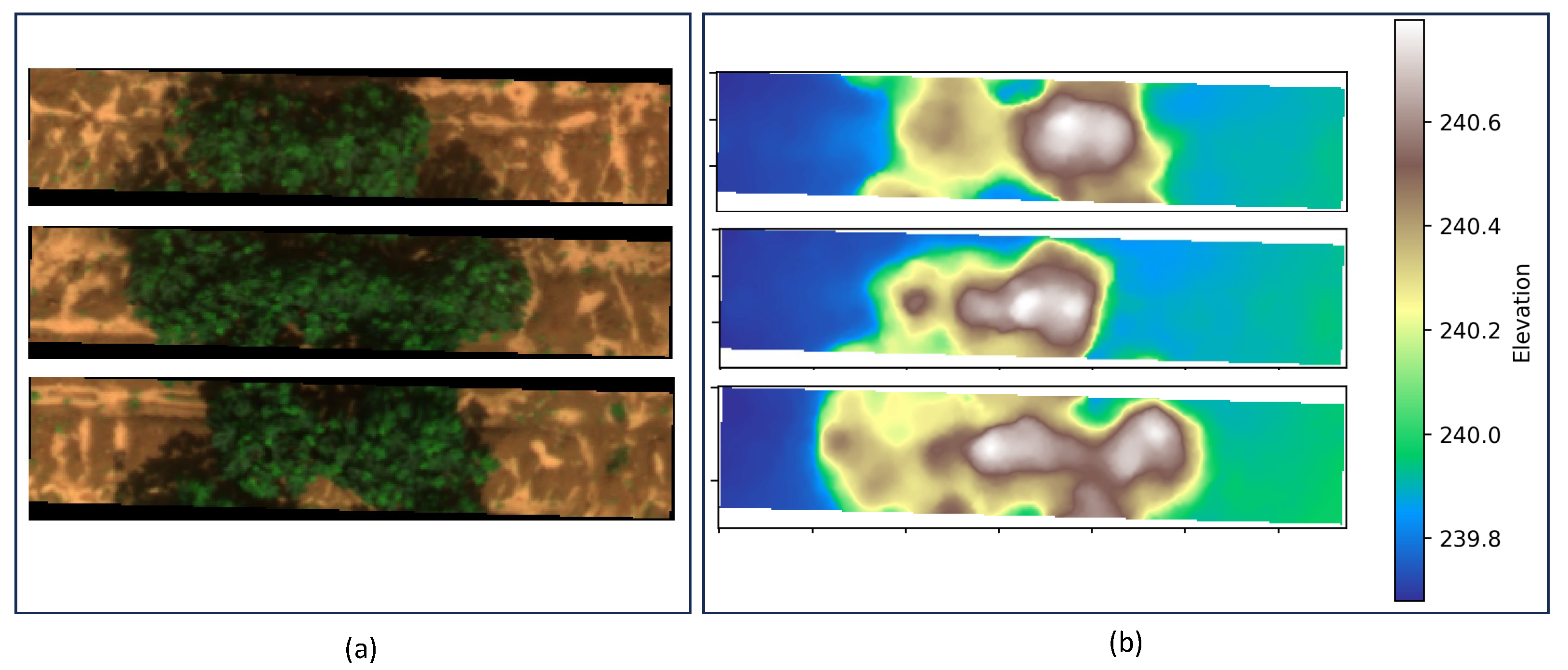
By mounting a multispectral camera on a drone, overlapping images of the field can be captured. These images can be processed using software such as DJI TERRA [4] to reconstruct both the Digital Elevation Model (DEM) and the multispectral image of the field. In the DEM, each pixel corresponds to an elevation. One traditional method for crop height prediction involves calculating the difference between the Digital Terrain Model (DTM)—representing the bare ground surface—and the DEM—signifying crop canopy elevation [5,6,7,8,9,10,11]—as depicted in Figure 1 and Figure 2. However, crop height derived from drone images is often shorter than the actual values [12], and the method itself is influenced by canopy density. As crop leaves expand, ground elevation data beneath the canopy become less visible, as shown in Figure 2b. In such cases, recovering the DTM or the ground 3D model becomes challenging.
In certain studies, Ground Calibration Targets (GCTs) have been used as references to address this issue [13,14]. For example, Han et al. [14] constructed wooden frames comprising ground, lower platform, and upper platform calibration points, serving as a semipermanent calibration system. Although using GCTs as references has demonstrated efficacy in specific contexts, this approach faces challenges in real-world farming scenarios, especially when fields span diverse terrains over extensive areas. Distinct terrains, including hilltops, slopes, and valleys, significantly influence the accuracy of canopy height calculations derived from drone images [15]. Generally, the traditional method of gathering spatial information remains labour-intensive and necessitates professional expertise. Moreover, the potential of using the multispectral image of the field for crop height estimation is still underexplored.
Actually, crop canopy reflectance captured via multispectral images is highly related to crop health and growth stages [16]. To be specific, Vegetation Indices (VIs), derived from mathematical formulations of canopy spectral reflectances, have a strong relation to specific characteristics in crops. Recently, some studies have used these specific VIs through machine learning methods to develop models for crop height prediction including wheat [17], maize [18], cotton [19], potatoes [20], and sunflower [21]. Unlike the traditional method that relies on preset models or equations, machine learning uses specific features as model input to calibrate and identify the most optimal parameters with the ground truth. However, traditional machine learning algorithms like support vector machines [22], random forests [23], and decision trees [24] often lack the capability to autonomously extract features from raw data. In the case of multispectral images, manually extracting correlated VIs is still necessary for predicting different crop heights. The manual feature selection approach often neglects variations in crop type, growth stage, and environmental influences on reflectance, which can impact model prediction accuracy. Moreover, the crucial DEM data, which are closely correlated to crop height, are frequently neglected.
To address these challenges, deep learning, a subset of machine learning with multiple layers, can automatically extract and learn features from multispectral images, which eliminates the need for manual feature selection. This adaptability enables the model to generalize across various crop types and growth stages, ensuring more consistent performance. Moreover, deep learning models can handle multiple data types, allowing both multispectral images and DEM to be used as model inputs. Some studies have used deep learning methods for crop classification [25], growth stage identification [26,27], disease detection [28], crop counts [29], weed detection [30], soil and crop segmentation [31], and yield prediction [32,33]. However, its application in crop height measurement using multispectral drone images remains a largely untapped area of research.
In general, the traditional method relies heavily on the generation of the DTM to obtain the difference between canopy elevation and ground elevation, which often suffers from the information beneath the canopy and varied terrains. Additionally, crop spectral reflectance, which is also related to crop height, is always overlooked. Machine learning provides solutions for using crop spectral reflectance to estimate crop height. However, its reliance on manual feature selection from multispectral images often neglects variances in crop type and growth stage. This oversight subsequently leads to variability in model performance across different crops and stages, and results can be inconsistent among different algorithms. Additionally, the significant DEM data, closely related to crop height, are frequently overlooked. Therefore, our objective is to find a solution that uses deep learning to automatically extract and learn features from both multispectral images and DEM to estimate crop height. This method aims to effectively use the DEM for capturing differences between canopy and ground elevations and terrain situations like slope and direction. Meanwhile, it incorporates multispectral images to identify potential VIs derived from crop spectral reflectance to distinguish between ground and crop regions and recognize different crop growth stages. We aim to overcome challenges including DTM generation, manual feature selection, and performance variability.
Based on the objective, we introduce a deep learning approach G-DMD that is based on Gated Recurrent Units (GRUs) [34] and uses DEM and multispectral drone images as model inputs to predict crop height. Inside the model, we combine a Convolutional Neural Network (CNN) [35] and GRUs for automatic feature extraction from inputs. The employment of GRUs enriches the model’s capability to analyse data with temporal dependencies, facilitating the recognition of long-term relationships between channels. Recognizing the unique characteristics of DEM and multispectral images, we introduce a data preparation process to enhance model learning efficacy. This method is adaptable to diverse terrains, various crop types, and all growth stages. It eliminates the need for manual GCP placement to gather additional ground information for DTM generation, as well as manual feature extraction from the inputs. Furthermore, the proposed approach allows for comprehensive surveying in each drone flight, facilitating accurate crop height assessments throughout the growing season while substantially reducing both labour and expertise requirements.
To evaluate the effectiveness of the G-DMD, we used a cotton dataset derived from Xu et al. [13], which comprises both DEM and multispectral images from a drone, correlated with on-ground measurements of both maximum and average cotton height. We began our evaluation with a comparison of the G-DMD against the traditional method. Subsequently, we demonstrated the enhancements brought by our visual data preparation process, underscoring its advantage in model learning performance. A baseline model without the GRU architecture was set to emphasize the robustness and advantages of adding GRU to the model structure. Our assessment also included testing the model with different input combinations such as only RGB, DEM, NIR, and RedEdge to highlight the importance of integrating both DEM and multispectral images. Evaluation results show that the G-DMD method significantly improved accuracy in measuring both maximum and average cotton height, with a 34% and 72% reduction in RMSE compared to the traditional method. Notably, the GRU-inclusive model achieved greater stability and accuracy during the training process and even showed slight outperformance in results compared to the GRU-exclusive model. Additionally, the combination of DEM and multispectral images achieved better results than any other single input. The contributions of our research are as follows:
- We develop the G-DMD as a method for crop height measurement using drone images. One of the main advantages is that our method does not require ground elevation information, i.e., DTM, eliminating the labour- and time-intensive process of gathering additional data. Meanwhile, this method has adaptability to diverse topographic landforms where the generation of DTMs often poses challenges to the precision of traditional techniques. Additionally, G-DMD negates the need for manual feature selection, and it becomes suitable for various crop types throughout their entire growth stages.
- We introduce the no-data value mask for the DEM, allowing the model to focus on the valuable parts of the DEM. This approach is essential as DEM data sometimes misses certain details. In addition to this, we present a separate normalization procedure for processing DEM and multispectral images as model inputs, addressing the different pixel characteristics between the two data types.
- We incorporate GRUs into our model after the CNN feature extraction layer to better capture the interchannel relationships among inputs. These inputs combine DEM data with spectral channels, each representing different segments of the electromagnetic spectrum. While CNNs are adept at discerning spatial hierarchies, they often lack in capturing sequential dependencies. Our evaluation results show that the addition of GRUs improves training stability. Additionally, combining DEM and multispectral image data as model inputs further boosts prediction accuracy.
- We evaluate and discuss the G-DMD, exploring its performance and potential applications in crop height measurement.
2. Materials and Methods
The G-DMD is designed to overcome the challenges associated with traditional crop height monitoring methods including the labour-intensive and time-consuming process of gathering additional information to build DTM and automatically extract features from inputs. It involves two main components: a unique data preparation method for DEM and multispectral images and a deep learning model based on GRU. The model is trained to automatically extract relevant features from inputs to regress actual crop heights. As a result, it offers not only a more precise prediction of crop height but also better applicability to varying topographic landforms without the necessity of DTMs.
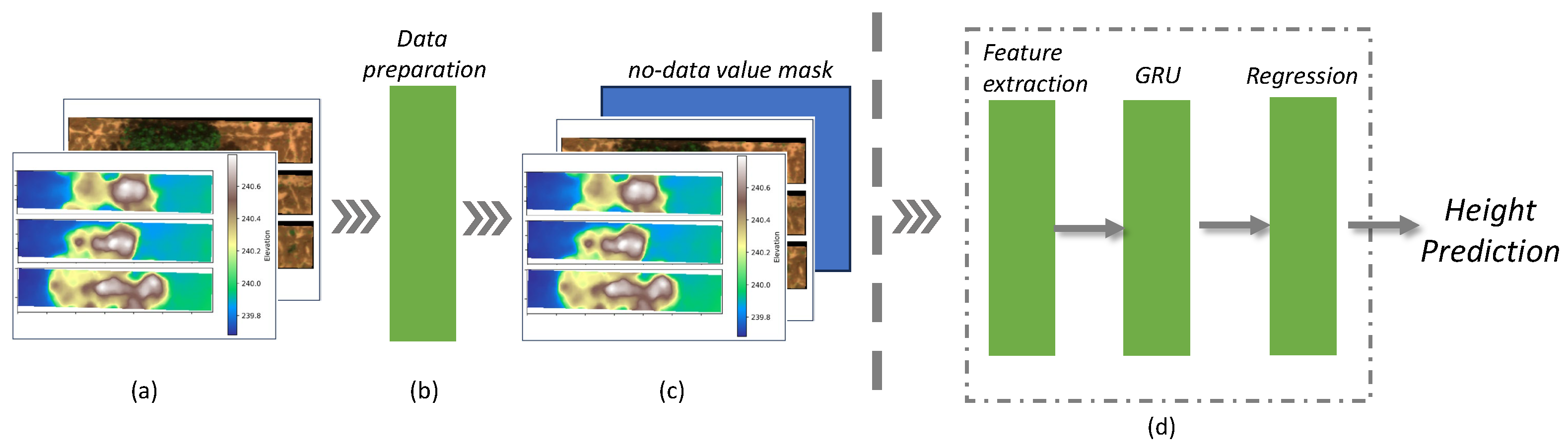
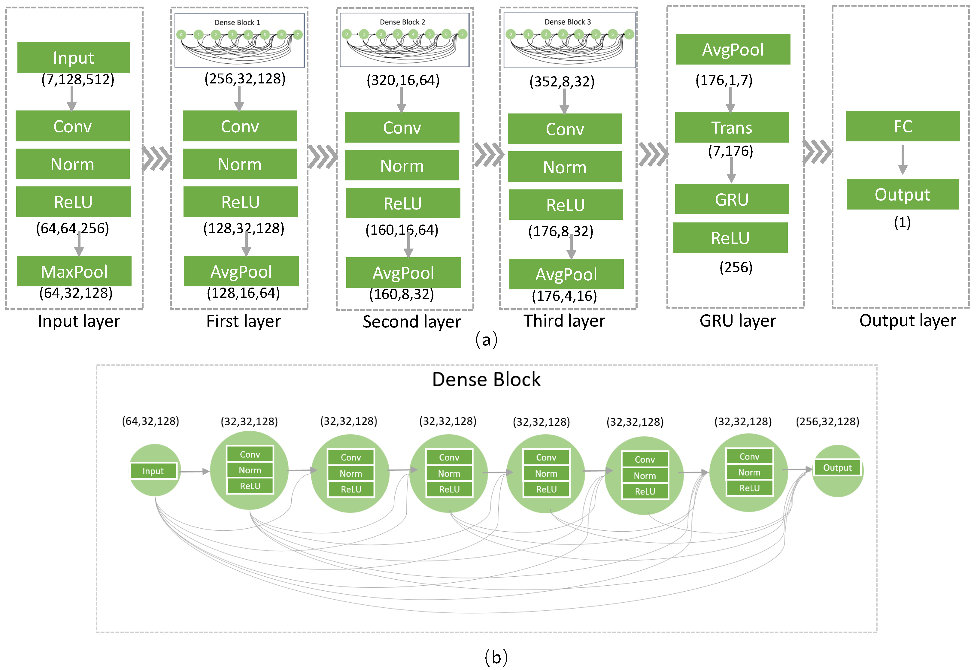
Figure 3 illustrates the comprehensive procedure of the G-DMD, encompassing both the data processing workflow and the deep learning model structure. In Figure 3a, the input data is displayed, which includes six channels: the DEM, blue, green, red, NIR, and RedEdge channels. Following the data preparation, as illustrated in Figure 3b, a mask is designed to address the missing information in the DEM. This is then incorporated into the dataset, followed by padding and data normalization. Figure 3c illustrates the prepared dataset. Finally, Figure 3d outlines the proposed deep learning model, which is composed of three integral components: feature extraction, GRUs, and the regression stage.
Section 2.1 discusses the data preparation, explaining the unique characteristics of the model inputs and the underlying principles that guide the data preparation process. Section 2.2 presents the feature extraction, detailing the model used for this purpose and explaining how it extracts features from the inputs. Section 2.3 discusses the principles of GRUs and how they contribute to enhancing model accuracy. Finally, Section 2.4 and Section 2.5 introduce the regression layer and the loss function, respectively.
2.1. Data Preparation
As part of the model inputs, DEM allows the deep learning model to learn the relationship between the DEM elevation and crop height at specific time points. This approach allows the model to distinguish terrain attributes like slope and orientation while understanding the correlation between plant height and the landscape, to predict plant height in specific situations. However, it faces challenges due to the nonlinear and dynamic progression of crop growth across varying temporal scales, which prevents the model from predicting crop height at different time points using only DEM features. Therefore, multispectral images are incorporated as part of the data inputs, enabling the model to identify different crop growth stages.
The DEM data provide continuous spatial information, capturing topographical variations within the landscape. However, like other Geographic Information System (GIS) data, the DEM also contains regions with no-data values, indicating either missing or obstructed information. Directly deleting the no-data values within the DEM data can cause confusion during the model training. This is because the deletion of these values may alter the spatial relationships and continuity in the data. In the PyTorch framework, positions that have been removed are not subject to updates during the model training process, potentially leading to prolonged training duration in our work. We first set all no-value data to zero to maintain consistency across the data and prevent potential computational issues during analysis. Then, we create a mask to identify these areas, as shown in Algorithm 1. In this mask layer, no-data values are represented by 1, and all other values are represented by 0. This layer allows the model to recognize and distinguish the no-value regions, preserving spatial relationships, and ensuring that subsequent analyses focus only on valid data from the DEM.
Additionally, the uniformity of input data size is a critical consideration for effective model training. The input data including the DEM and multispectral image are padded into the same dimension of .
Data normalization, a vital preprocessing technique, has proven to be efficient in deep learning models. By scaling all features to a uniform range, normalization mitigates issues related to the scale sensitivity, preventing one feature from dominating others. Meanwhile, it can accelerate the convergence to reduce the training time [36]. The Mini-Max Scaler is chosen for data normalization, as it maintains the original shape of the distribution. In our method, we differentiate between the DEM and other spectral channels, treating them as separate entities in the preprocessing stage. The DEM represents topographical information with unique scaling and distribution characteristics, while other channels may correspond to various spectral or radiometric attributes. Given these differences, we use separate normalization procedures for the DEM and other channels. This method enhances the model’s ability to capture between topographical and spectral features, thereby facilitating a more accurate and comprehensive analysis. Similarly, we extend this normalization approach to the ground truth data in our study. While this method has the advantage of enhancing the efficiency and coherence of model training, it may lead to a temporary reduction in interpretability as the original scales of the values are transformed. However, this concern is addressed in the prediction phase of our analysis. By employing a denormalization algorithm, the model can directly predict the actual heights from the input images, thereby translating the normalized predictions back into the real-world context.
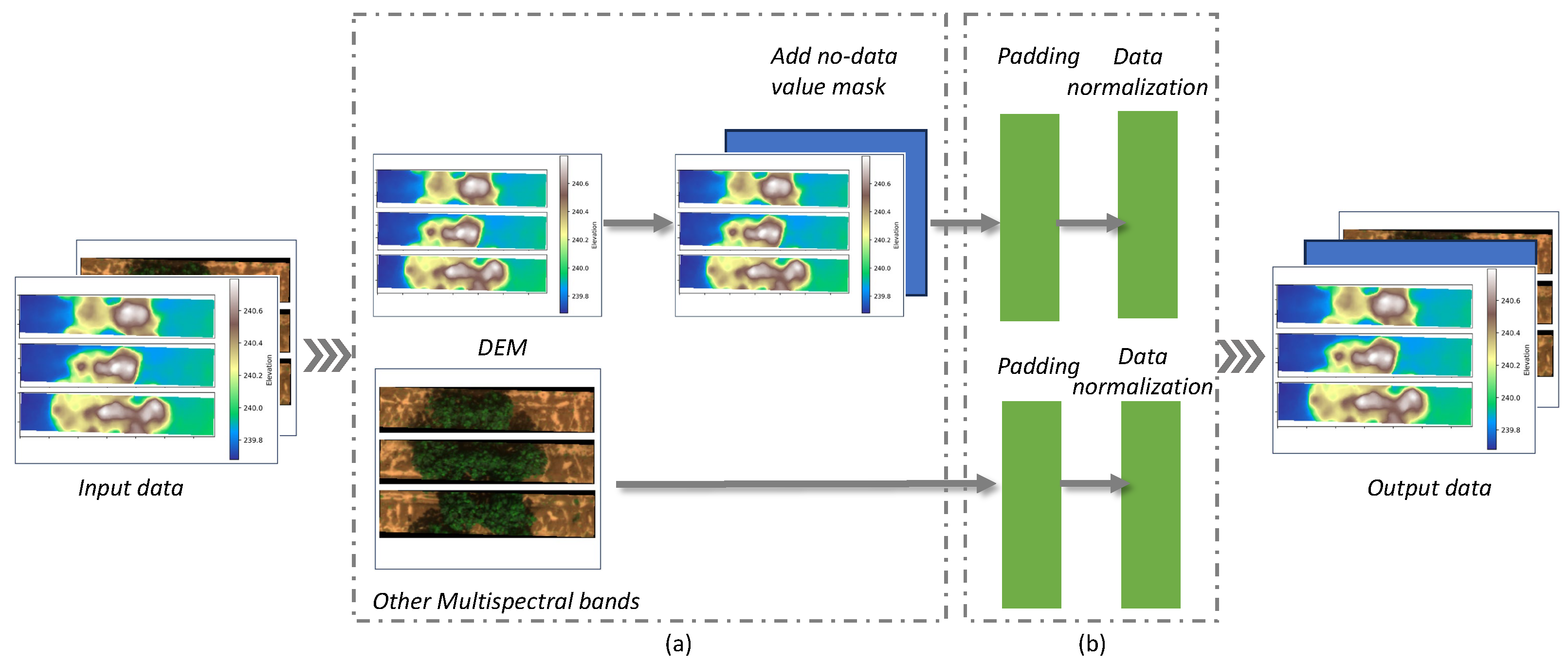
The data preparation process is illustrated in Figure 4. Initially, input data are divided into the DEM channel and other multispectral image channels. Then, the no-data value mask is added to enable the deep learning model to better understand the data. Subsequently, the DEM channel and other multispectral image channels undergo separate padding and normalization processes to ensure uniformity and that all input features are on a similar scale.
During the training process, we employed data augmentation techniques including random horizontal flips, vertical flips, and rotations on the DEM data and colour adjustments including brightness, contrast, saturation, and hue throughout the training epochs for the multispectral images.
| Algorithm 1: No-data value mask |
|
2.2. Feature Extraction
The feature extraction part plays a crucial role in transforming the prepared input dataset, which includes the DEM and multispectral images, into a set of meaningful and informative features. The feature extraction process involves reducing the dimensionality of the input data while retaining the most important and informative attributes for crop height prediction. This process focuses on the critical attributes of the data, such as edges, corners, and textures, and enhances the speed and efficiency of the model. Ultimately, the extracted feature set is fed into the subsequent stages of the model—GRUs and regression stage—for further analysis and final crop height prediction.
In the feature extraction process, the Convolutional Neural Network (CNN) [35] is used because of its proficiency in automatically learning and extracting features from images, eliminating the need for traditional manual feature extraction. Specifically, our study aims to infer the crop growth stages and establish the relationship between crop height and ground elevation in different terrain characteristics using the DEM and multispectral images from a drone. The DEM provides terrain characteristics, while the multispectral images capture the crop growth stages. Additionally, the CNN possesses translational invariance, which can recognize the same features across different positions in an image. This capability of the CNN, combined with the comprehensive input data, enables the extraction of intricate features and relationships essential for understanding crop growth stages and their relationship with ground elevation.
In this research, the feature extraction network structure is inspired by the Dense Connectivity Network (DenseNet) [37], which has achieved good results in classification. Compared to a single CNN layer, a comprehensive network framework typically includes multiple convolutional layers, activation functions, and pooling layers. This complexity helps the model learn more intricate and rich feature representations from raw image data, capturing hierarchical structures that a single CNN layer might fail to grasp. Additionally, complete network frameworks are often adaptable to various tasks and datasets which is a crucial aspect in handling the specific requirements in this research. Compared to previously published networks such as ResNet [38], VGG [39], and Inception [40], the fundamental idea behind the DenseNet is the dense connections, as shown in Figure 5b. Firstly, the Dense Block lets each layer use features from previous layers, which helps gather detailed features. This accumulation of features helps to capture intricate details and relationships between terrain characteristics and crop growth stages. Secondly, the Dense Blocks enhance the gradient flow throughout the network, mitigating issues related to vanishing gradients and thus making it possible to train deeper models effectively. This is particularly important when dealing with multitemporal, multispectral data where capturing complex patterns becomes essential. Finally, the Dense Blocks provide a parameter-efficient design. Their ability to facilitate efficient feature extraction and feature reuse allows us to achieve high accuracy while keeping the model size relatively small. Therefore, the inclusion of the Dense Blocks serves to enrich the feature extraction capability of our model, making it more effective and efficient in predicting crop height based on complex, multisource data. Figure 5 demonstrates the feature extraction network, comprising the first, second, and third layers, each containing a Dense Block. A Dense Block consists of six consecutive convolutional processes, where the input is combined with the previous output before each process.
As illustrated in Figure 5a, the initial step involves padding the DEM and multispectral image data to ensure uniformity, resulting in input samples with dimensions of , where 7 represents input channels and represents input dimension. These samples are then processed via consecutive convolution layers to obtain a size of . After a max pooling process, the size is reduced to , which is then passed through the first Dense Block, as shown in Figure 5b. This Dense Block contains six basic convolution processes, each consisting of convolution, normalization, and Rectified Linear Unit (ReLU) activation functions. Each basic convolution processes all the previous outputs. After the first Dense Block, the feature map changes to 256 features with a size of , and then, following another basic process including convolution, normalization, ReLU, and average pooling, the size changes to 128 features with a size of . After the third layer process, the size is transformed to . Subsequently, these embedding data are fed into a GRU layer, enabling the model to learn the sequential relationships within the data. From the GRU module, a new embedding with a dimension of 256 is obtained. This is then passed into an output layer to predict the crop height.
2.3. GRU-Based Modelling
The initial feature extraction through the DenseNet is pivotal for the model as it helps spatial relationships and complicated patterns within each individual channel. In this research, the input data include the DEM and five specific spectral channels from multispectral images. These inputs capture discrete portions of the electromagnetic spectrum, thereby encompassing both spatial and contextual features [41].
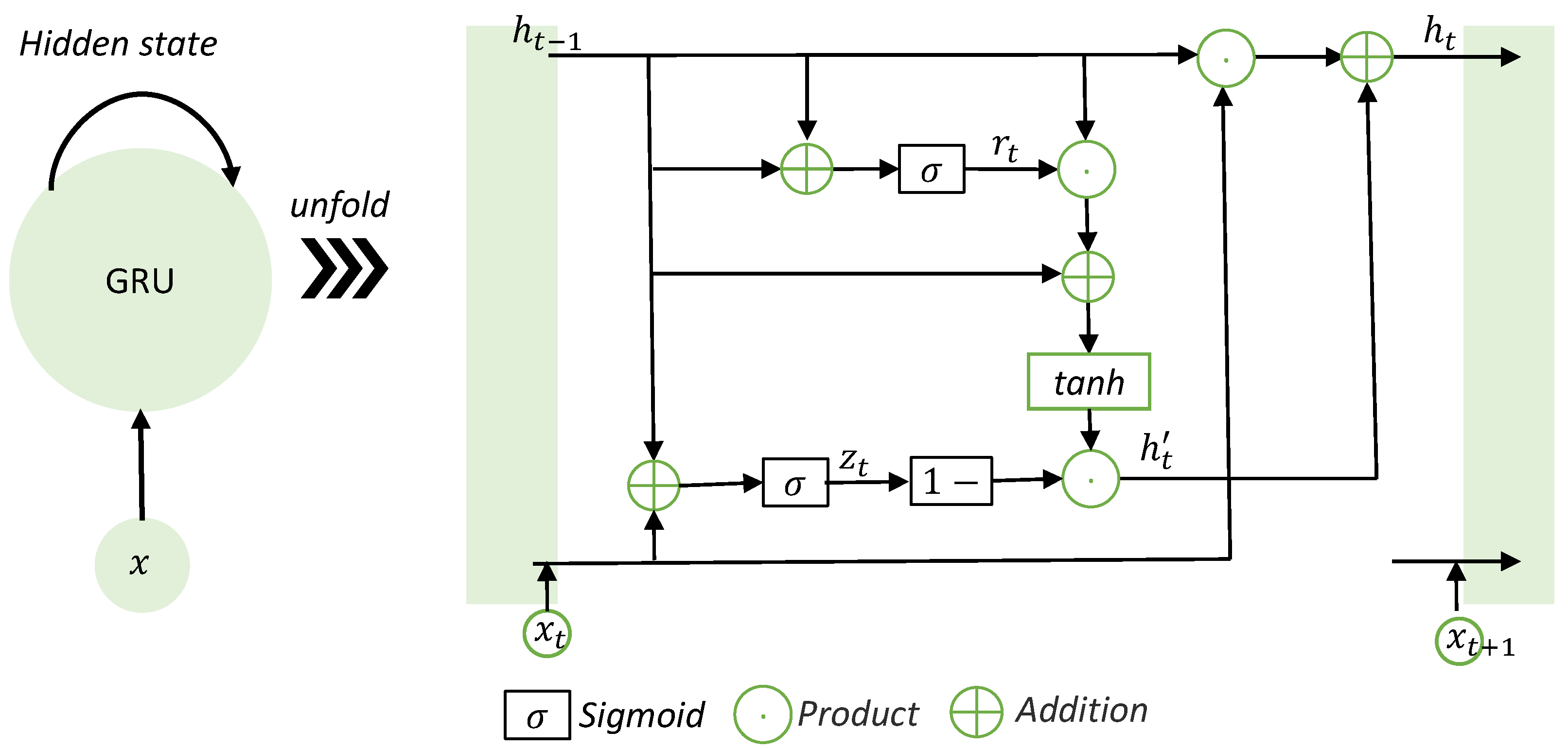
In order to optimally capture the nonlinear relationship between the extracted features and crop height, a GRU layer is integrated into the feature extraction network. The GRU is proficient in identifying dependencies and sequential patterns across different channels, effectively marrying the spatial characteristics with the unique relationships potentially existing among DEM and multispectral image data. This is accomplished by incorporating a gate structure, inspired by neurons, which facilitates the continuous transmission of sequence states from the preceding stages [42].
The Gated Recurrent Unit (GRU) [34] is a type of Recurrent Neural Network (RNN) [43] that is capable of learning long-term dependencies in sequence data. The traditional RNN faces challenges when processing data with long-term dependencies as it is difficult to capture patterns that span extended sequences [44]. Compared to the Long Short-Term Memory unit (LSTM) [45] and the Transformer [46], the GRU has a simpler architecture with fewer parameters which can lead to faster training times and reduce computational power needs. Our research aims to find the relationships among the input channels, so using LSTMs or Transformers might be excessive, especially when the input sequences are relatively short.
In Figure 6, a detailed depiction of information transmission for feature points at different positions in the GRU space is presented. The GRU consists of two main gates: the reset gate and the update gate , as shown in the following Equations (1) and (2). The updated gate helps the model to decide how much of the past information from the hidden state needs to be passed along to the future. This is important for capturing dependencies over different time steps. The reset gate helps the model to decide how much of the past information needs to be forgotten. The gates are regulated by the sigmoid activation function, which compresses values into a range between 0 to 1, allowing them to be interpreted as probabilities. This is crucial for the model to not remember unnecessary information from the past. is the current memory content which is a candidate hidden state that includes the current input and the past hidden state (modulated by the reset gate). The function used in Equation (3) scales the values to be in the range of to 1, which can help the model to learn and converge faster as the values are centred around 0. is the final memory at the current time step which is a combination of the past hidden state and the candidate hidden state, modulated by the updated gate as shown in Equation (4). This helps the model decide on the final memory at the current time step, taking into account the past hidden state, the current candidate memory content, and the update gate.
In preparation for the GRU module, the dimensions of the input are transformed from to as shown in Figure 5’s ‘GRU layer’ section. This transformation is achieved by applying average pooling over the appropriate dimensions, resulting in 7 time steps and 176 features for each time step. Subsequently, these data are processed by the GRU module with a hidden state size of 256, ultimately producing 256 features as output.
where represents the input at time t; are the weight matrices for the input ; are the weight matrices for the previous hidden state ; are the bias terms; represents the sigmoid activation function; represents the hyperbolic tangent activation function; and ⊙ represents element-wise multiplication [34].
2.4. Regression Layer
Subsequent to the GRU layer, a regression layer is incorporated into the model. This layer is crucial for refining the high-dimensional output from the GRU layer and regressing it to the actual crop height. More specifically, the regression layer employs a fully connected (FC) layer to ensure that the model’s output is consistent with the expected range and distribution of crop heights, as illustrated in the ‘Output layer’ section of Figure 5, where the dimensions are transformed from 256 to 1.
2.5. Loss Function
The MSE (Mean Squared Error) as shown in Equation (5) is chosen as the loss function in our study which is calculated as the average of the squared differences between the ground truth and predicted values for crop height.
where is the actual value of the data point, is the predicted value of the data point, and n is the total number of data points.
3. Results
In this section, we introduce the details of dataset preparation, the experimental environment, evaluations, and the obtained results. In Section 3.1, we present the dataset and processing methodologies. Section 3.2 outlines our experimental environment, the parameter configurations, and the evaluation indexes. Section 3.3 draws a comparison between the G-DMD and the traditional method. Section 3.4 shows the significance of the introduced no-data value mask using heat maps. Section 3.5 presents outcomes from the model without normalization. Section 3.6 compares the G-DMD with a model without GRU layers. Finally, Section 3.7 compares varied input channels.
3.1. Dataset
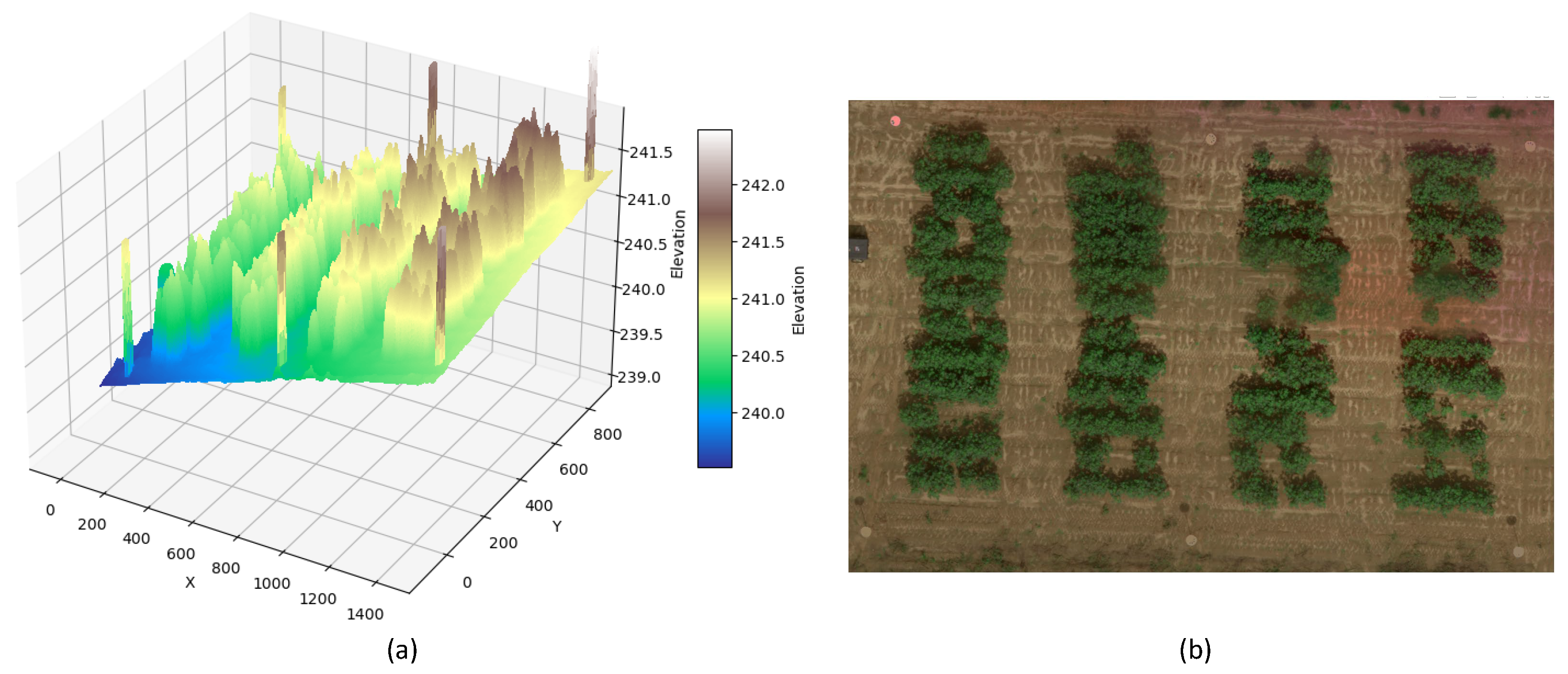
In this paper, we use the dataset collected by Xu et al. [13] which is published in Figshare [47]. These data were collected at the University of Georgia Plant Sciences Farm in Watkinsville, GA, encompassing 48 plots, each 3 m long and 0.9 m wide. Height measurements of each plant within the plots were manually recorded on six separate occasions. The data collection was divided into two segments: 48 plots were measured twice, and 24 plots were measured four times, due to the tractor’s rolling pattern. Images of the experimental field were captured via an Octocopter (s1000+, DJI) equipped with a lightweight multispectral camera (RedEdge, MicaSense) at a speed of 2.5 m/s and a height of 20 m above ground level. The software/services PhotoScan and MicaSense ATLASGigital were used to create the DEMs and orthomosaic images as depicted in Figure 7. Each DEM pixel represents elevation, while the orthomosaic image is an overlaying of blue, green, red, NIR, and RedEdge bands. Overall, the dataset consists of six cotton field DEMs and orthomosaic images, as shown in Figure 7, alongside 192 plot height data records.
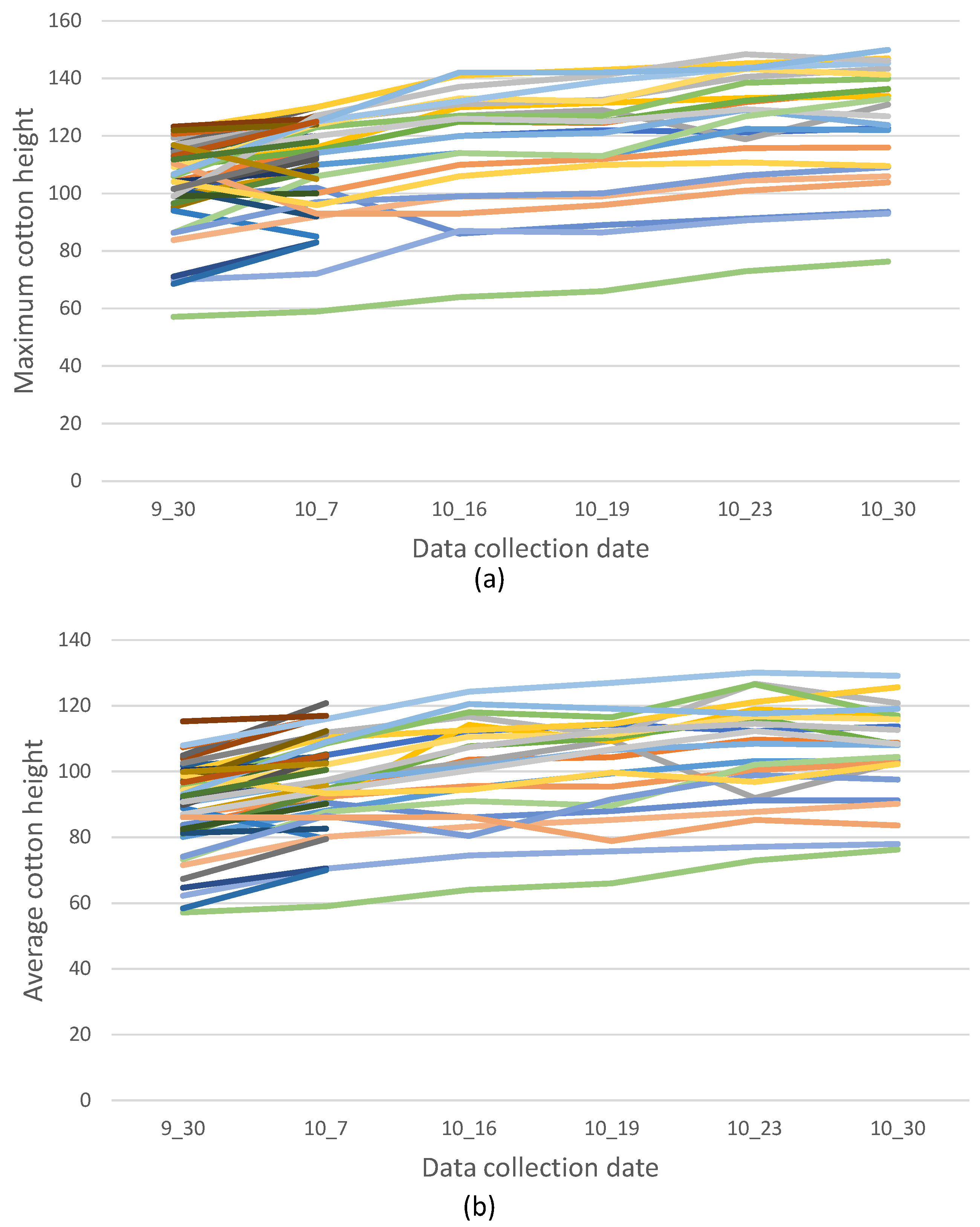
In this research, we have further processed the data to suit our study’s objectives. Specifically, we focus on the maximum and average cotton height within each plot. The trends in maximum and average cotton height across the data collection dates are illustrated in Figure 8. Each line in the figure represents maximum and average cotton height changes during the measurement dates in one plot. Notably, the dates 30 September (9_30) and 7 October (10_7) have 48 plots, while other dates have 24 plots. Additionally, we have divided the DEM and orthomosaic images into plot segments using the QGIS software [48]. This division allows us to correlate each plot with the corresponding maximum and average cotton height ground truth. Some examples of these plot images can be seen in Figure 9.
The dataset is separated into training, validation, and test datasets according to a stratified sampling method, ensuring that each subset retains the same proportion of dates as present in the original dataset. The distribution is as follows: the training subset encompasses 60% with 115 samples; the validation and test subsets each consist of 20%, tallying 38 and 39 samples, respectively.
3.2. Configuration
We used the Python programming language and the Rasterio and Sklearn packages to read, process, and save the dataset. Model training was conducted on a DELL Academ-J7G2SV3 with Intel (R) Xeon (R) W-11955M CPU with 32.0 GB RAM and NVIDIA RTX A3000. The deep learning model was built in Pytorch. The optimizer used to train the model was Adam, the initial learning rate was 0.001, the batch size was 4, and the total epoch was 300. In DenseNet, the growth rate was set at 32. The architecture comprised three blocks, with each block containing six layers. The GRU’s hidden size was configured to 256, and it consisted of four stacked layers. These settings helped manage the increasing complexity as the network deepened, ensuring effective feature extraction. For the subsequent experiments, the model was trained from scratch. A total of 192 samples were used for the experiment, of which 115 samples were selected as the training data, 38 samples were used as the validation dataset, and 39 samples were used as the testing dataset.
To assess the accuracy of the predicted value and ground truth, the Root Mean Square Error (RMSE) and Mean Absolute Error (MAE) shown in Equations (6) and (7) were used as evaluation metrics. The RMSE measures the average difference between the predicted values and the corresponding ground truth values. A lower RMSE indicates a more accurate prediction of the cotton plant height using the model. MAE calculates the average of the absolute differences between the actual values and predicted values, intuitively reflecting the magnitude of the prediction error.
where is the observed value, is the predicted value, and n is the number of observations.
3.3. Comparison with Traditional Method
As previously mentioned, the conventional approach for obtaining crop height involves using a DEM to construct a 3D model of the ground surface as DTM, where the difference between the z-coordinates of the model is considered as the crop height. We used the cotton dataset to reproduce the traditional method in the following steps [13]:
- Generate the DEM and orthomosaic images from drone images and separate them into plots. The pixel values of the DEM present the cotton and ground elevations.
- Calculate the cotton height. (a) Separate the ground and cotton according to the Normalized Difference Vegetation Index (NDVI) value. (b) Build the point cloud model of the ground to find the fitted plane to represent the ground surface. (c) Calculate the difference in elevation between the ground plane surface, i.e., DTM, and cotton canopy, i.e., DSM, to calculate the maximum and average cotton height of each plot.
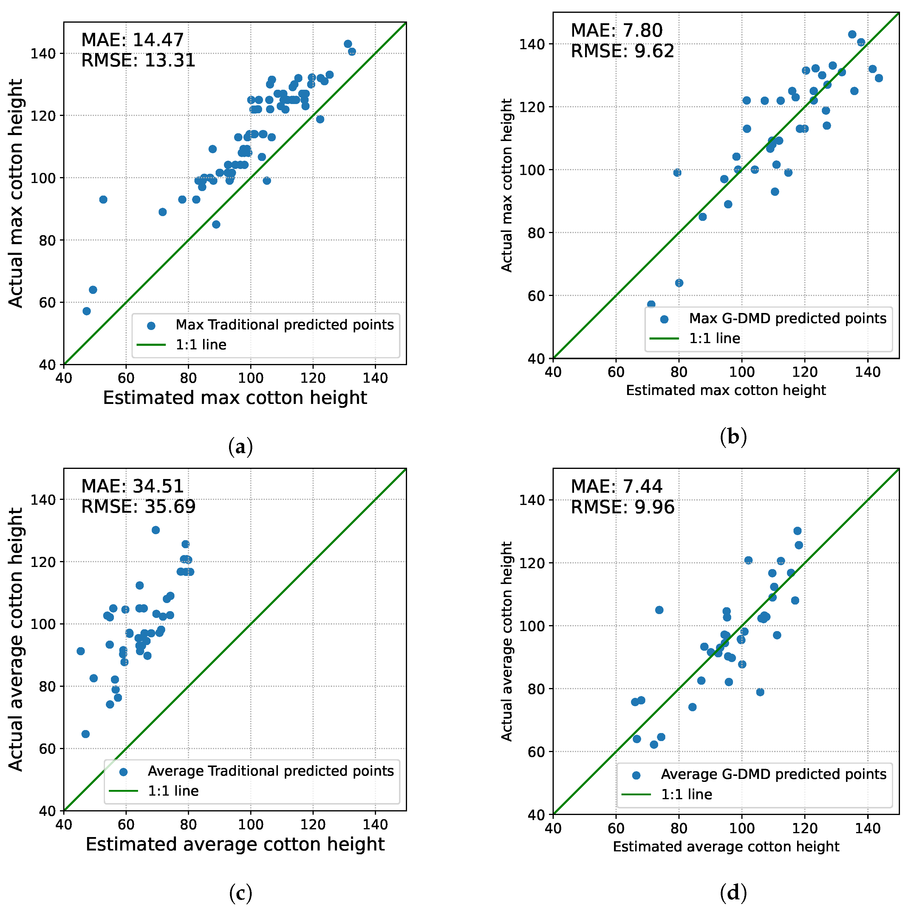
We used the G-DMD to train the model for maximum and average cotton height prediction separately. The test dataset was used to evaluate the G-DMD and the traditional method results. We used the RMSE and MAE to test the accuracy of these two methods. The results are shown in Table 1 and Table 2.
In the comparison of maximum cotton height, as shown in Table 1, the advanced capabilities of the G-DMD method in predicting crop height became apparent. Compared to the traditional method, the G-DMD showcased its refined predictive capability, reducing the RMSE to 9.62 cm from the 14.47 cm observed in the traditional method—a 33.5% improvement. Similarly, the MAE also significantly declined, achieving 7.8 cm for the G-DMD, a 41.4% improvement from the 13.31 cm of the traditional approach.
When assessing the prediction of average cotton height as shown in Table 2, the advantages of the G-DMD method become even more significant. The RMSE for the G-DMD is recorded at 9.96 cm, marking a 72.1% decrease relative to the 35.69 cm RMSE of the traditional approach. Similarly, the MAE highlighted the G-DMD’s enhanced precision, achieving 7.44 cm compared to the traditional method’s 34.51 cm—a reduction of 78.4%.
Figure 10 presents scatter plots comparing the predicted versus actual cotton height for both maximum and average measures. The x-axis denotes the estimated cotton height, while the y-axis illustrates the actual measurements. In Figure 10a, the dispersion of prediction points from the 1:1 line underscores the variability in the traditional method’s estimation of maximum cotton height. Conversely, Figure 10b reveals a tighter clustering of points around the 1:1 line, signifying the superior accuracy of the G-DMD method for maximum height prediction. Similarly, Figure 10c,d contrast the performance of the traditional and G-DMD methods in predicting average cotton height. While the traditional method seems to be more accurate for maximum cotton height than for the average height, the G-DMD method consistently exhibits stability in its RMSE and MAE predictions across both measures.
3.4. Comparison with the No-Data Value Mask
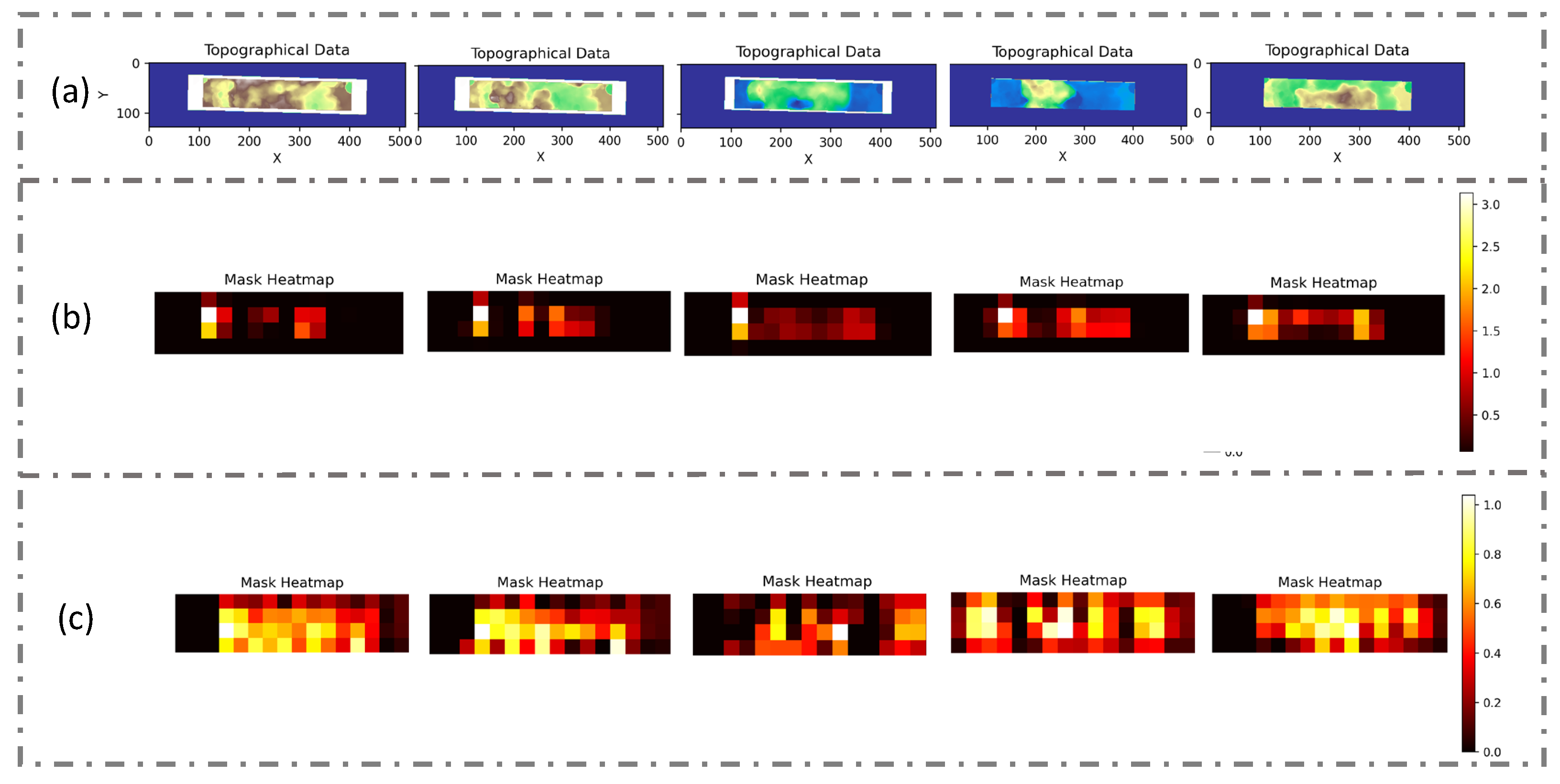
In this evaluation, heat maps were used to provide an intuitive depiction of the model’s learning progression, particularly when the no-data value mask was incorporated into the input dataset. This no-data value mask was specifically designed to pinpoint invalid data within the DEM, thereby enabling the model to discern the true characteristics of the terrain with greater accuracy and faster speed. By adopting this strategy, the model was able to concentrate on the vital information contained within the DEM images, whilst simultaneously disregarding the invalid data that might otherwise have led to erroneous interpretations. For this reason, in this experiment, we used the presetting parameters, but only the DEM channel was used as the input, and we compared the input with and without the no-data value mask. Moreover, we arranged the input data into the model in sequence, allowing us to track the trend of the heat maps in the same input DEM.
The heat maps were generated after 100 epochs of training because, by this point, the model was likely to have either reached convergence or be nearing it, signifying a stabilization in its parameter and weight updates. The findings are illustrated in Figure 11. Figure 11a displays the original DEM input, with lighter shades representing higher elevations. To maintain uniformity in the size of the input DEM, the image was padded to a dimension of 512 × 128, with the padded areas highlighted in blue. Figure 11b reveals the heat map corresponding to the input with the no-data value mask after 100 epochs of training, while Figure 11c shows the heat map for the input without the no-data value mask after 100 epochs.
During training, the use of the no-data value mask led to a heightened heat index and concentrated the model’s attention on pertinent parts of the image, effectively excluding the padded regions. In contrast, the model without the mask dispersed its focus onto the padded parts. One potential reason for this performance difference is that the mask aids the model in distinctly differentiating between data points and no-data points, thus sharpening its focus on valid data. Additionally, the mask layer might enable the model to filter out irrelevant noise during training, allowing for greater concentration on essential features.
3.5. Comparison with the Non-Normalization Method
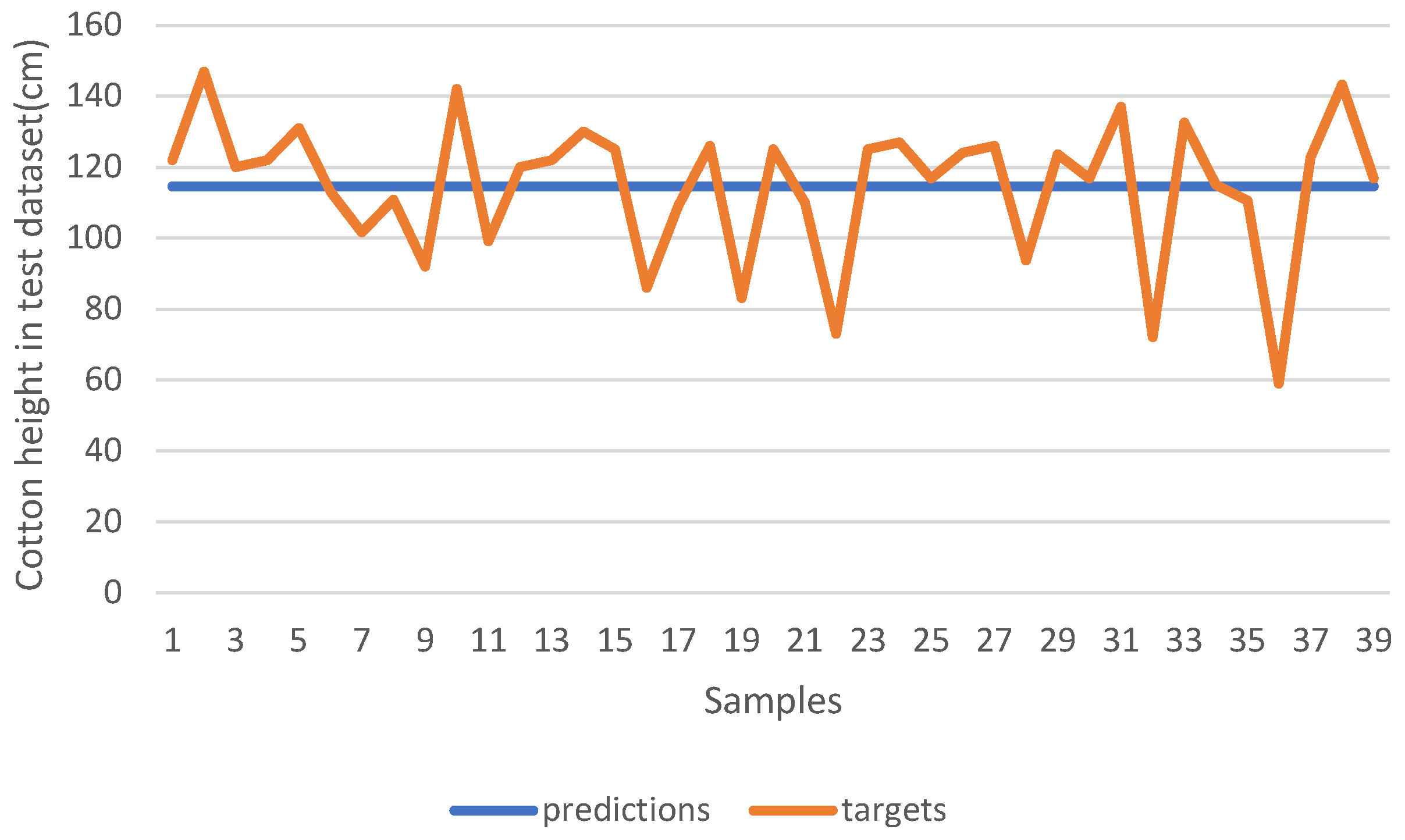
In this part, we use an experiment to show the significance of data normalization in the context of training a model for cotton height prediction. While prior research has suggested that data normalization can save training time and enhance accuracy, this method often falls short in providing an intuitive demonstration of the process during both training and prediction stages. In our method, we first used data normalization for DEM and multispectral images separately and then extended the renormalization process during prediction, allowing for a more precise and intuitive representation of the results.
We trained the model using the input dataset without normalization; the results are shown in Figure 12. The blue line shows the model prediction in the test dataset, and the orange line shows the ground truth. It is observed that the model outputs consistent results across different input samples. The lack of normalization appears to cause the model to converge on predictions of uniform values to minimize the overall training loss. This phenomenon occurs because, when data are not normalized, large feature values can dominate the loss calculation. Consequently, the model predominantly focuses on these large-scale features and tends to neglect others. While predicting a constant value may reduce this dominant loss, it fails to exhibit robust generalization across varied data points, leading to compromised model accuracy.
3.6. Comparison with a Model without GRU Layer
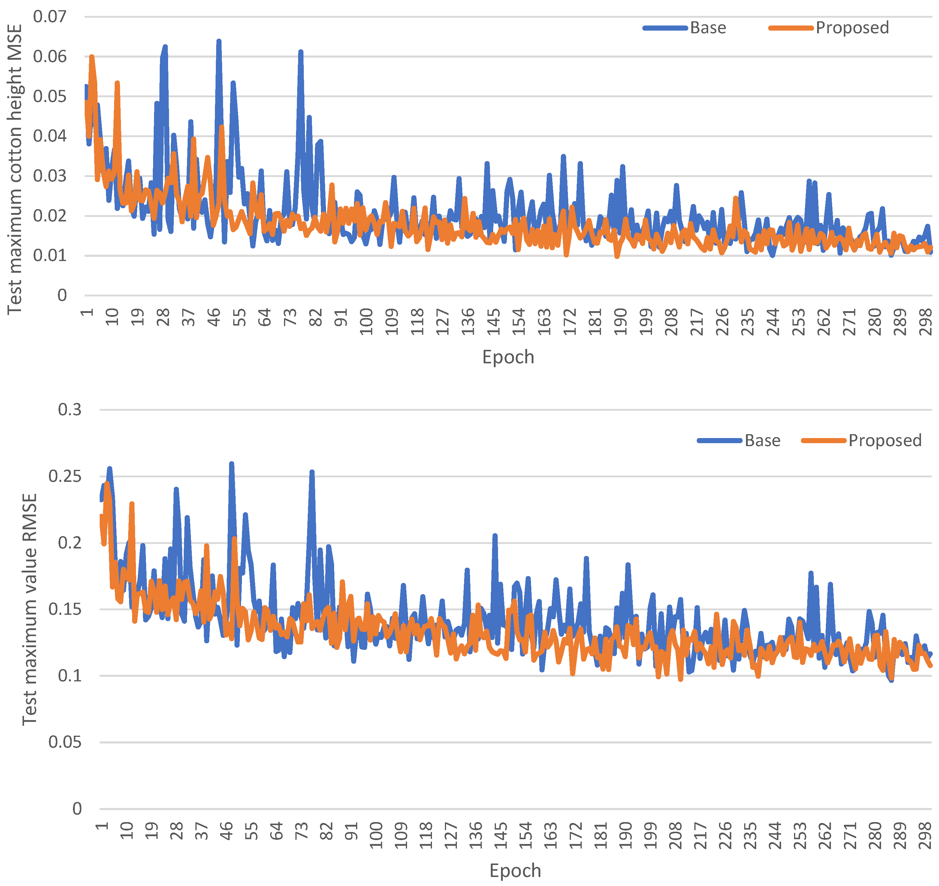
To assess the value of the GRU structure, we compared its performance with a simplified network, hereafter referred to as the ‘base’ model. This ‘base’ model consists of only a feature extraction network and a regression module. Other factors, such as variations in optimization algorithms and learning rates, are kept the same. We aimed to isolate the specific contributions of the GRU to prediction accuracy. During this investigation, we monitored the model’s response on the test dataset throughout its training, recording the results at each epoch to provide a clearer understanding of its performance trajectory and the GRU’s incremental benefits.
Figure 13 presents a comparative analysis of the MSE and RMSE for two distinct models: the ‘base’ model and our proposed model. The x-axis represents the training epochs, while the y-axis illustrates the corresponding MSE values and RMSE values. In the experimental results, the ‘base’ model, represented by the blue line, demonstrates a slower rate of decline in both RMSE and MSE compared to our proposed model, depicted by the yellow line. Moreover, the error of the model prediction in the test dataset exhibits greater stability than the ‘base’ model. This disparity in convergence speed may be attributed to the enhanced capability of our proposed method, which employs the GRU structure, to capture the complex patterns and characteristics inherent in the data.
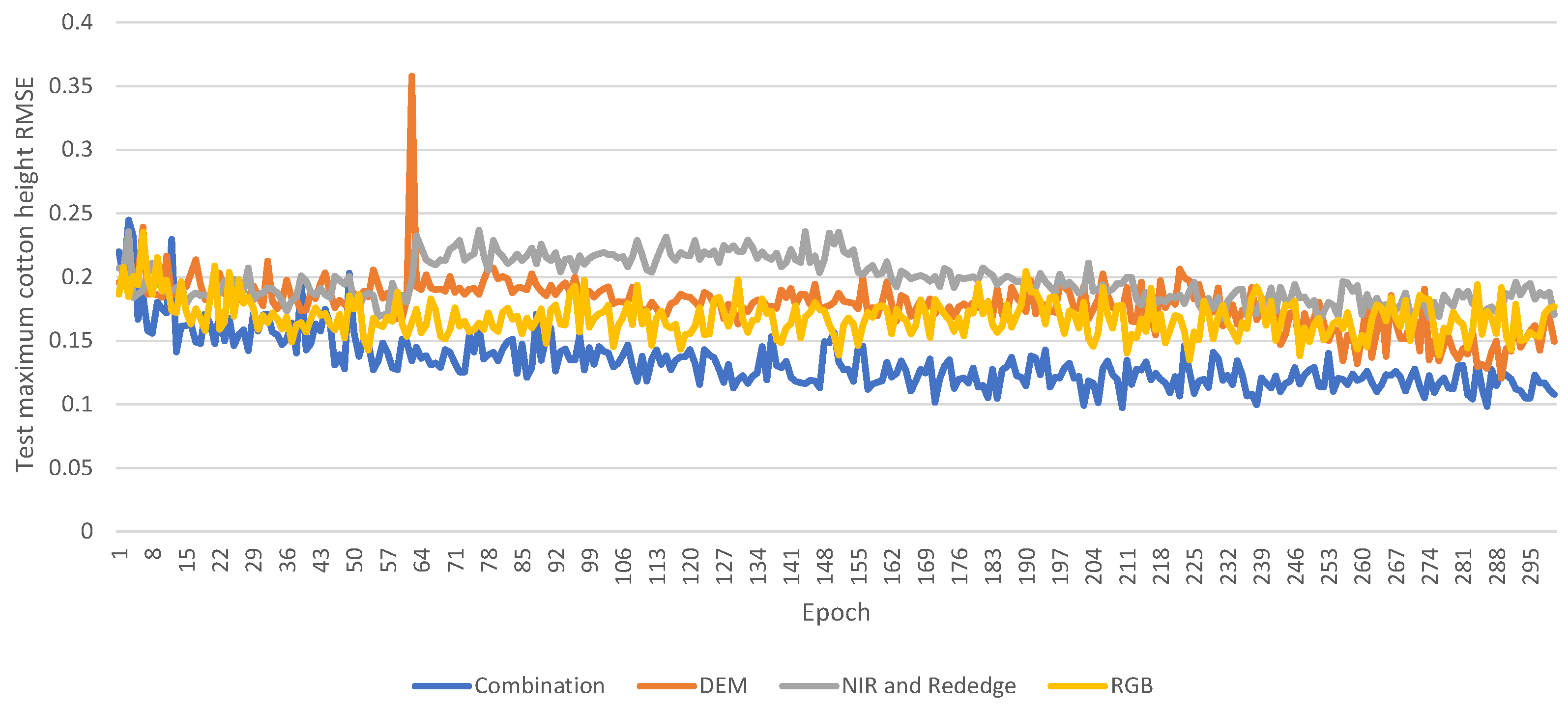
3.7. Comparison with Different Input Channels
To investigate the complex relationships between different input features and their influence on model learning, we conducted a series of experiments using various input channels, i.e., DEM, RGB, NIR, RedEdge, and a combination of all, with the model to determine which kind of combination of channels is the most influential in accurately predicting crop height. The model trained 300 epochs for each set of input channels, and the test dataset was used to assess the model’s quality. Table 3 shows the results with the test dataset after renormalization. Figure 14 shows the trend of RMSE on the test dataset during training. Since the test dataset remained invisible during training, the model’s performance on this test set provides insights into its potential accuracy in real-world applications.
The results demonstrate that the input combining all channels presents the most accurate predictions. During the training, this combination exhibits a stable decline in RMSE on the test dataset. In each training epoch, it consistently outperforms other input methods by registering the lowest error on the test dataset. This improved performance can be attributed to the complementary information that each channel—DEM, RGB, NIR, and RedEdge—provides about the terrain and crops. By integrating all channels, the model benefits from a richer set of features, which capture different facets of the crops and enhance its predictive capabilities. Moreover, combining data from diverse channels can counterbalance any noise or errors inherent to individual channels. This is because inconsistencies or noise in one channel might be offset by reliable signals from others. In general, each channel offers insights into specific terrain attributes and the growth stages. Consequently, using multiple channels as model inputs provides a more robust prediction of cotton height, effectively associating them with terrain attributes and growth stages.
4. Discussion
Our findings highlight the potential of using the DEM and multispectral images from a drone to measure crop height, particularly in real agricultural contexts. This approach enables crop height prediction without the necessity for ground elevation information, which is often obscured by crop foliage in real-world scenarios. This obstruction typically necessitates additional spatial information to reconstruct the DTM to calculate the difference in z-coordinates between ground and canopy elevation, a process that is both time-consuming and labour-intensive.
We use the no-value mask during data preparation to process the unique characteristics of DEM data and use the heat map to assess its efficacy. Our primary objective is not merely to enhance accuracy through the no-value mask but to ensure the model focuses on crucial input segments and achieves faster convergence. The result presented in Section 3.4, as illustrated by the heat maps, confirms that the model focuses on pertinent terrain features due to the incorporation of the no-value mask.
Additionally, due to the distinct characteristics of the DEM, multispectral images, and ground truth, we apply normalization separately to each component and renormalize the output using the previous scaler, resulting in predictions more closely aligned with reality.
In the evaluation of the ‘base’ network, our attention is directed towards the test dataset’s performance during training epochs. We also implement the GRU to identify the relationships between channels, particularly in multispectral images, where temporal correlations often exist. Experiment results indicate that this approach contributes to the model’s stability.
In selecting input data channels, we determine that using multiple channels, including the DEM, RGB, NIR, and RedEdge, facilitates more precise cotton height predictions than previous research.
In the cotton dataset, while the maximum and average cotton height RMSE errors of the G-DMD model are 9.62 cm and 9.96 cm, they are still 38% lower for maximum cotton height and 72% lower for average cotton height compared to the traditional method. One reason for this discrepancy is the error associated with the manual measurement of cotton ground truth data. As observed in Figure 8, the maximum and average heights in each plot do not exhibit consistent growth, and in some instances, the height even decreases over time, which indicates possible errors in manual measurement. Another factor is the small size of the cotton dataset, increasing the likelihood of overfitting.
Our findings corroborate the results presented by Malachy et al. [49], where the RMSE errors for the traditional method in measuring maximum cotton, tomato, and potato height are 25 cm, 19 cm, and 11 cm and for average height are 32 cm, 29 cm, and 13 cm. These results are similar to our experiments for the traditional method, where the RMSE for maximum cotton height is 14 cm and for average cotton height is 35 cm. While Malachy et al. observe reduced errors after optimizing their machine learning approach with actual data, this optimization compromises the model’s transferability, necessitating actual data from new fields for result adjustment. In contrast, our method produces results without the need for secondary optimization. When compared with the actual cotton height of around 70–100 cm in the dataset we used, the error margin remains within an acceptable threshold. Moreover, a study by Valluvan et al. [50] highlights that the traditional method’s accuracy in determining crop height is impacted due to slope variations. Despite using a linear model for ground elevation adjustment, their reported RMSE error for maize crop height remains around 14.17 cm.
Meanwhile, our findings are in agreement with the study by Da Silva Andrea et al. [19] which tested different machine learning algorithms combined with different manual feature selections using satellite multispectral imagery for cotton height prediction during the entire growing season and obtained MAE errors ranging from 8 to 25 cm. Moreover, Osco et al. [18] reported RMSE errors between 17 cm and 30 cm for maize plant height predictions using drone multispectral images, combined with machine learning methodologies and manual feature extraction.
Our findings provide valuable guidance for agricultural crop height monitoring. By integrating both elevation and multispectral image data, we aim to increase the model’s adaptability in different scenarios, which is to be tested in our future work.
Finally, since these experimental results are specific to the cotton dataset, generalizing these findings requires caution. Variations in crop types or crop average height could result in different outcomes, thus emphasizing the need for additional research to thoroughly understand the automatic solution for crop height monitoring. Future studies should extend this exploration with larger crop datasets, aiming to train the model with transfer learning for different real scenarios. While the results are promising, further studies could explore the application of this model to other crops and varied geographical regions.
5. Conclusions
In this paper, we introduce the G-DMD, an approach for crop height measurement in real agriculture scenarios based on a deep learning model that autonomously extracts features from the multispectral images and DEM. Our approach obviates the need for ground elevation information, specifically the DTM, thereby overcoming the labour- and time-consuming process of gathering additional data. Moreover, the G-DMD is adaptable across various topographic landforms, addressing accuracy issues often encountered in traditional methods due to errors in DTM reconstruction. Importantly, we use a deep learning method to autonomously extract and learn features from raw data, including multispectral images and DEM obtained from drone imagery. This approach overcomes the accuracy uncertainties associated with manual feature selection across different crop types and growth stages. We add a GRU layer after CNN-based feature extraction to better capture features across varied characteristic inputs. Simultaneously, we introduce a data preparation process for both the DEM and multispectral images, optimizing the extraction of diverse features from these inputs.
Evaluation results confirm that the G-DMD predicts crop height with an acceptable RMSE error in the test dataset, outperforming the traditional method with around 38% lower error for maximum cotton height and 72% lower error for average cotton height. The incorporation of GRUs in the model resulted in a more stable training process on the test dataset. The evaluation also revealed that the combination of inputs (DEM and multispectral images) yielded superior results compared to single-input models. While this study focused solely on the cotton dataset, the entire process we detailed—from preparing the dataset to training and prediction—can be applied to other datasets. While the model’s adaptability to other datasets has not yet been explored, our next step is to expand our research to different datasets, aiming to enhance the robustness and generalizability of the G-DMD. This method has held promise for automatic crop height monitoring in agricultural settings.
As agriculture continues to evolve towards more automated crop monitoring, the demand for efficient and automated solutions for crop height measurement will become increasingly important. Our work highlights the potential of advanced deep learning techniques to enhance agricultural practices.
Author Contributions
Conceptualization, methodology, software, validation, formal analysis, investigation, resources, writing—original draft preparation, writing—review and editing, visualization, J.W. Writing—review and editing, N.O. Review, P.B. Review and supervision, B.K.N. All authors have read and agreed to the published version of the manuscript.
Funding
This research was funded by the University of Sussex.
Data Availability Statement
The original dataset used in this study is openly accessible and was obtained from the work of Xu et al. [13] published in Figshare [47]. For researchers interested in the implementation details and the processed data, the corresponding code and dataset are available upon request from the corresponding author.
Acknowledgments
We extend our heartfelt gratitude to Xu et al. [13] for generously providing the foundational dataset for this research.
Conflicts of Interest
The authors declare no conflict of interest.
Abbreviations
The following abbreviations are used in this manuscript:
| DEM | Digital Elevation Model |
| DTM | Digital Terrain Model |
| CNN | Convolutional Neural Network |
| RNN | Recurrent Neural Network |
| GRU | Gated Recurrent Unit |
| DenseNet | Dense Connectivity Network |
| ReLU | Rectified Linear Unit |
| GCP | Ground Control Point |
| VIs | Vegetation Indices |
| GCT | Ground Calibration Target |
| NIR | Near-Infrared |
| MSE | Mean Squared Error |
| RMSE | Root Mean Square Error |
| MAE | Mean Absolute Error |
References
- Chang, A.; Jung, J.; Maeda, M.M.; Landivar, J. Crop height monitoring with digital imagery from Unmanned Aerial System (UAS). Comput. Electron. Agric. 2017, 141, 232–237. [Google Scholar] [CrossRef]
- ten Harkel, J.; Bartholomeus, H.; Kooistra, L. Biomass and crop height estimation of different crops using UAV-based LiDAR. Remote Sens. 2019, 12, 17. [Google Scholar] [CrossRef]
- Bendig, J.; Yu, K.; Aasen, H.; Bolten, A.; Bennertz, S.; Broscheit, J.; Gnyp, M.L.; Bareth, G. Combining UAV-based plant height from crop surface models, visible, and near infrared vegetation indices for biomass monitoring in barley. Int. J. Appl. Earth Obs. Geoinf. 2015, 39, 79–87. [Google Scholar] [CrossRef]
- DJI. DJI Terra, Version 2021.05. 2021. Available online: https://www.dji.com/uk/dji-terra/info (accessed on 1 August 2023).
- Wang, J.; Zhao, X.; Zhao, D.; Triantafilis, J. Selecting optimal calibration samples using proximal sensing EM induction and γ-ray spectrometry data: An application to managing lime and magnesium in sugarcane growing soil. J. Environ. Manag. 2021, 296, 113357. [Google Scholar] [CrossRef] [PubMed]
- Rueda-Ayala, V.P.; Peña, J.M.; Höglind, M.; Bengochea-Guevara, J.M.; Andújar, D. Comparing UAV-based technologies and RGB-D reconstruction methods for plant height and biomass monitoring on grass ley. Sensors 2019, 19, 535. [Google Scholar] [CrossRef]
- Wijesingha, J.; Moeckel, T.; Hensgen, F.; Wachendorf, M. Evaluation of 3D point cloud-based models for the prediction of grassland biomass. Int. J. Appl. Earth Obs. Geoinf. 2019, 78, 352–359. [Google Scholar] [CrossRef]
- Oliveira, R.A.; Näsi, R.; Niemeläinen, O.; Nyholm, L.; Alhonoja, K.; Kaivosoja, J.; Jauhiainen, L.; Viljanen, N.; Nezami, S.; Markelin, L.; et al. Machine learning estimators for the quantity and quality of grass swards used for silage production using drone-based imaging spectrometry and photogrammetry. Remote Sens. Environ. 2020, 246, 111830. [Google Scholar] [CrossRef]
- Pranga, J.; Borra-Serrano, I.; Aper, J.; De Swaef, T.; Ghesquiere, A.; Quataert, P.; Roldán-Ruiz, I.; Janssens, I.A.; Ruysschaert, G.; Lootens, P. Improving accuracy of herbage yield predictions in perennial ryegrass with uav-based structural and spectral data fusion and machine learning. Remote Sens. 2021, 13, 3459. [Google Scholar] [CrossRef]
- Bareth, G.; Schellberg, J. Replacing manual rising plate meter measurements with low-cost UAV-derived sward height data in grasslands for spatial monitoring. PFG-Photogramm. Remote Sens. Geoinf. Sci. 2018, 86, 157–168. [Google Scholar] [CrossRef]
- Belton, D.; Helmholz, P.; Long, J.; Zerihun, A. Crop height monitoring using a consumer-grade camera and UAV technology. PFG-Photogramm. Remote Sens. Geoinf. Sci. 2019, 87, 249–262. [Google Scholar] [CrossRef]
- Maimaitijiang, M.; Sagan, V.; Sidike, P.; Daloye, A.M.; Erkbol, H.; Fritschi, F.B. Crop monitoring using satellite/UAV data fusion and machine learning. Remote Sens. 2020, 12, 1357. [Google Scholar] [CrossRef]
- Xu, R.; Li, C.; Paterson, A.H. Multispectral imaging and unmanned aerial systems for cotton plant phenotyping. PLoS ONE 2019, 14, e0205083. [Google Scholar] [CrossRef]
- Han, X.; Thomasson, J.A.; Bagnall, G.C.; Pugh, N.A.; Horne, D.W.; Rooney, W.L.; Jung, J.; Chang, A.; Malambo, L.; Popescu, S.C.; et al. Measurement and calibration of plant-height from fixed-wing UAV images. Sensors 2018, 18, 4092. [Google Scholar] [CrossRef]
- Miura, N.; Yamada, S.; Niwa, Y. Estimation of canopy height and biomass of Miscanthus sinensis in semi-natural grassland using time-series UAV data. ISPRS Ann. Photogramm. Remote Sens. Spat. Inf. Sci. 2020, 3, 497–503. [Google Scholar] [CrossRef]
- Miller, J.J.; Schepers, J.S.; Shapiro, C.A.; Arneson, N.J.; Eskridge, K.M.; Oliveira, M.C.; Giesler, L.J. Characterizing soybean vigor and productivity using multiple crop canopy sensor readings. Field Crops Res. 2018, 216, 22–31. [Google Scholar] [CrossRef]
- Zhen, Z.; Yunsheng, L.; Moses, O.A.; Rui, L.; Li, M.; Jun, L. Hyperspectral vegetation indexes to monitor wheat plant height under different sowing conditions. Spectrosc. Lett. 2020, 53, 194–206. [Google Scholar] [CrossRef]
- Osco, L.P.; Junior, J.M.; Ramos, A.P.M.; Furuya, D.E.G.; Santana, D.C.; Teodoro, L.P.R.; Gonçalves, W.N.; Baio, F.H.R.; Pistori, H.; Junior, C.A.d.S.; et al. Leaf nitrogen concentration and plant height prediction for maize using UAV-based multispectral imagery and machine learning techniques. Remote Sens. 2020, 12, 3237. [Google Scholar] [CrossRef]
- da Silva Andrea, M.C.; de Oliveira Nascimento, J.P.F.; Mota, F.C.M.; de Souza Oliveira, R. Predictive framework of plant height in commercial cotton fields using a remote sensing and machine learning approach. Smart Agric. Technol. 2023, 4, 100154. [Google Scholar] [CrossRef]
- Papadavid, G.; Hadjimitsis, D.; Toulios, L.; Michaelides, S. Mapping potato crop height and leaf area index through vegetation indices using remote sensing in Cyprus. J. Appl. Remote Sens. 2011, 5, 053526. [Google Scholar] [CrossRef]
- Abdikan, S.; Sekertekin, A.; Narin, O.G.; Delen, A.; Sanli, F.B. A comparative analysis of SLR, MLR, ANN, XGBoost and CNN for crop height estimation of sunflower using Sentinel-1 and Sentinel-2. Adv. Space Res. 2023, 71, 3045–3059. [Google Scholar] [CrossRef]
- Hearst, M.A.; Dumais, S.T.; Osuna, E.; Platt, J.; Scholkopf, B. Support vector machines. IEEE Intell. Syst. Their Appl. 1998, 13, 18–28. [Google Scholar] [CrossRef]
- Breiman, L. Random forests. Mach. Learn. 2001, 45, 5–32. [Google Scholar] [CrossRef]
- Kingsford, C.; Salzberg, S.L. What are decision trees? Nat. Biotechnol. 2008, 26, 1011–1013. [Google Scholar] [CrossRef]
- Fan, C.; Lu, R. UAV image crop classification based on deep learning with spatial and spectral features. IOP Conf. Ser. Earth Environ. Sci. 2021, 783, 012080. [Google Scholar] [CrossRef]
- Zhong, L.; Hu, L.; Zhou, H. Deep learning based multi-temporal crop classification. Remote Sens. Environ. 2019, 221, 430–443. [Google Scholar] [CrossRef]
- Lu, X.; Zhou, J.; Yang, R.; Yan, Z.; Lin, Y.; Jiao, J.; Liu, F. Automated Rice Phenology Stage Mapping Using UAV Images and Deep Learning. Drones 2023, 7, 83. [Google Scholar] [CrossRef]
- Shahi, T.B.; Xu, C.Y.; Neupane, A.; Guo, W. Recent Advances in Crop Disease Detection Using UAV and Deep Learning Techniques. Remote Sens. 2023, 15, 2450. [Google Scholar] [CrossRef]
- Vong, C.N.; Conway, L.S.; Zhou, J.; Kitchen, N.R.; Sudduth, K.A. Early corn stand count of different cropping systems using UAV-imagery and deep learning. Comput. Electron. Agric. 2021, 186, 106214. [Google Scholar] [CrossRef]
- Wang, J.; Yao, X.; Nguyen, B.K. Identification and localisation of multiple weeds in grassland for removal operation. In Proceedings of the Fourteenth International Conference on Digital Image Processing (ICDIP 2022), Wuhan, China, 20–23 May 2022; Volume 12342, pp. 290–299. [Google Scholar]
- Dyson, J.; Mancini, A.; Frontoni, E.; Zingaretti, P. Deep learning for soil and crop segmentation from remotely sensed data. Remote Sens. 2019, 11, 1859. [Google Scholar] [CrossRef]
- Maimaitijiang, M.; Sagan, V.; Sidike, P.; Hartling, S.; Esposito, F.; Fritschi, F.B. Soybean yield prediction from UAV using multimodal data fusion and deep learning. Remote Sens. Environ. 2020, 237, 111599. [Google Scholar] [CrossRef]
- Muruganantham, P.; Wibowo, S.; Grandhi, S.; Samrat, N.H.; Islam, N. A systematic literature review on crop yield prediction with deep learning and remote sensing. Remote Sens. 2022, 14, 1990. [Google Scholar] [CrossRef]
- Dey, R.; Salem, F.M. Gate-variants of gated recurrent unit (GRU) neural networks. In Proceedings of the 2017 IEEE 60th International Midwest Symposium on Circuits and Systems (MWSCAS), Boston, MA, USA, 6–9 August 2017; pp. 1597–1600. [Google Scholar]
- Russakovsky, O.; Deng, J.; Su, H.; Krause, J.; Satheesh, S.; Ma, S.; Huang, Z.; Karpathy, A.; Khosla, A.; Bernstein, M.; et al. Imagenet large scale visual recognition challenge. Int. J. Comput. Vis. 2015, 115, 211–252. [Google Scholar] [CrossRef]
- Ali, P.J.M.; Faraj, R.H.; Koya, E.; Ali, P.J.M.; Faraj, R.H. Data normalization and standardization: A technical report. Mach. Learn. Tech. Rep. 2014, 1, 1–6. [Google Scholar]
- Huang, G.; Liu, Z.; Van Der Maaten, L.; Weinberger, K.Q. Densely connected convolutional networks. In Proceedings of the IEEE Conference on Computer Vision and Pattern Recognition, Honolulu, HI, USA, 21–26 July 2017; pp. 4700–4708. [Google Scholar]
- He, K.; Zhang, X.; Ren, S.; Sun, J. Deep residual learning for image recognition. In Proceedings of the IEEE Conference on Computer Vision and Pattern Recognition, Las Vegas, NV, USA, 26 June–1 July 2016; pp. 770–778. [Google Scholar]
- Simonyan, K.; Zisserman, A. Very deep convolutional networks for large-scale image recognition. arXiv 2014, arXiv:1409.1556. [Google Scholar]
- Szegedy, C.; Liu, W.; Jia, Y.; Sermanet, P.; Reed, S.; Anguelov, D.; Erhan, D.; Vanhoucke, V.; Rabinovich, A. Going deeper with convolutions. In Proceedings of the IEEE Conference on Computer Vision and Pattern Recognition, Boston, MA, USA, 7–12 June 2015; pp. 1–9. [Google Scholar]
- Liang, L.; Zhang, S.; Li, J. Multiscale DenseNet meets with bi-RNN for hyperspectral image classification. IEEE J. Sel. Top. Appl. Earth Obs. Remote Sens. 2022, 15, 5401–5415. [Google Scholar] [CrossRef]
- Sherstinsky, A. Fundamentals of recurrent neural network (RNN) and long short-term memory (LSTM) network. Phys. D Nonlinear Phenom. 2020, 404, 132306. [Google Scholar] [CrossRef]
- Schuster, M.; Paliwal, K.K. Bidirectional recurrent neural networks. IEEE Trans. Signal Process. 1997, 45, 2673–2681. [Google Scholar] [CrossRef]
- Elman, J.L. Finding structure in time. Cogn. Sci. 1990, 14, 179–211. [Google Scholar] [CrossRef]
- Hochreiter, S.; Schmidhuber, J. Long short-term memory. Neural Comput. 1997, 9, 1735–1780. [Google Scholar] [CrossRef]
- Vaswani, A.; Shazeer, N.; Parmar, N.; Uszkoreit, J.; Jones, L.; Gomez, A.N.; Kaiser, Ł; Polosukhin, I. Attention is all you need. In Advances in Neural Information Processing Systems 30 (NIPS 2017); Curran Associates, Inc.: Red Hook, NY, USA, 2017; Volume 30. [Google Scholar]
- Xu, R.; Li, C.; Paterson, A.H. UAV Multispectral. Figshare. Dataset. 2018. Available online: https://figshare.com/articles/dataset/UAV_multispectral/7122143/1 (accessed on 1 August 2023).
- QGIS Development Team. QGIS Geographic Information System, Version 3.16; QGIS Development Team: Bern, Switzerland, 2021. [Google Scholar]
- Malachy, N.; Zadak, I.; Rozenstein, O. Comparing methods to extract crop height and estimate crop coefficient from UAV imagery using structure from motion. Remote Sens. 2022, 14, 810. [Google Scholar] [CrossRef]
- Valluvan, A.B.; Raj, R.; Pingale, R.; Jagarlapudi, A. Canopy height estimation using drone-based RGB images. Smart Agric. Technol. 2023, 4, 100145. [Google Scholar] [CrossRef]
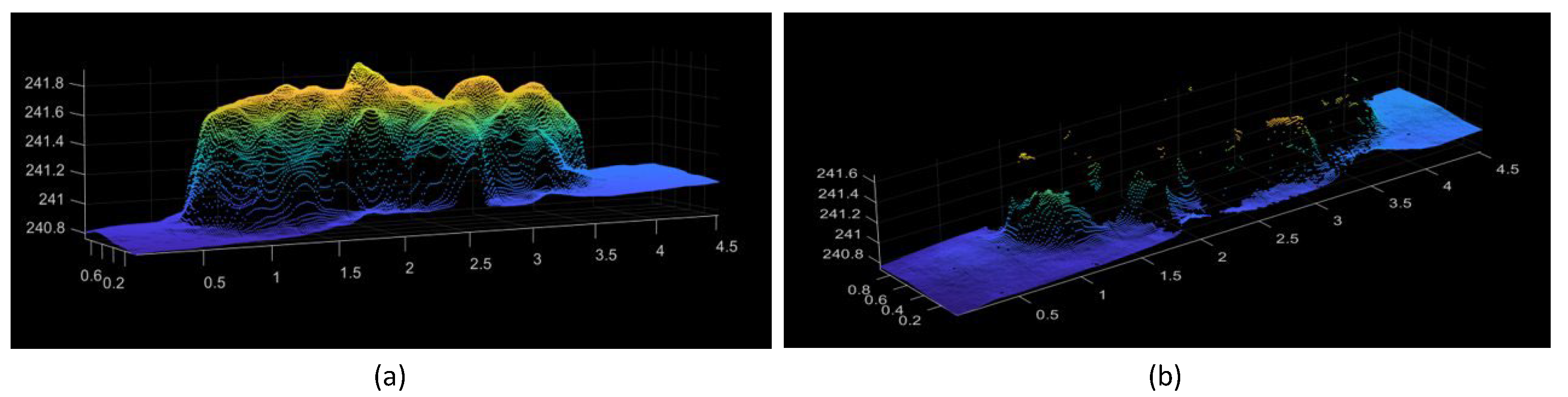
Figure 1.
Visualization of 3D models of the canopy and ground surfaces [13]. (a) DEM—representing the elevation of the crop canopy. (b) DTM—representing the bare ground surface, with only ground points remaining.
Figure 1.
Visualization of 3D models of the canopy and ground surfaces [13]. (a) DEM—representing the elevation of the crop canopy. (b) DTM—representing the bare ground surface, with only ground points remaining.

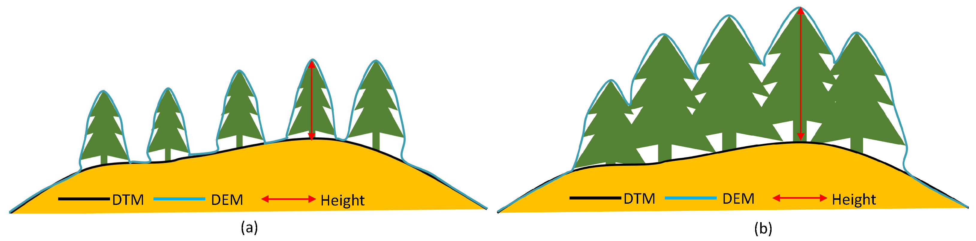
Figure 2.
Illustration of crop height calculation derived from the difference between DEM and DTM. (a) A scenario where the crop canopy does not cover the ground. (b) A scenario where the crop canopy tends to cover the ground, resulting in the loss of ground elevation information.
Figure 2.
Illustration of crop height calculation derived from the difference between DEM and DTM. (a) A scenario where the crop canopy does not cover the ground. (b) A scenario where the crop canopy tends to cover the ground, resulting in the loss of ground elevation information.

Figure 3.
Overview of G-DMD, including data preparation and deep learning model structure. (a) Input dataset consisting of six channels: DEM, blue, green, red, NIR, and RedEdge channels. (b) Data preparation step which includes the incorporation of a no-data value mask into the DEM channel, followed by padding and data normalization. (c) The prepared input dataset with seven channels. (d) Proposed deep learning model composed of feature extraction, GRUs, and regression stage.

Figure 4.
Data preparation process. (a) The input data are separated into the DEM channel and other multispectral image channels, followed by the application of a no-data value mask to the DEM. (b) DEM channel and multispectral image channels are then subjected to padding and normalization separately.

Figure 5.
Depiction of the deep learning model incorporating layers for feature extraction (from input layer section to third layer section), GRUs, and regression. (a) The proposed architecture with input dimensions , where 7 signifies the number of channels and represents the image size. (b) The structure of the Dense Block.

Figure 6.
Diagrammatic representation of a Gated Recurrent Unit (GRU).

Figure 7.
Sample DEM and orthomosaic image from the experimental field. (a) A 3D visualization of the DEM. (b) RGB components of the orthomosaic image [13].
Figure 7.
Sample DEM and orthomosaic image from the experimental field. (a) A 3D visualization of the DEM. (b) RGB components of the orthomosaic image [13].

Figure 8.
The cotton height trend in each plot. (a) The maximum cotton height trend in each plot. (b) The average cotton height trend in each plot.
Figure 8.
The cotton height trend in each plot. (a) The maximum cotton height trend in each plot. (b) The average cotton height trend in each plot.

Figure 9.
Some input samples from the dataset. (a) RGB plot segments. (b) DEM plot segments.

Figure 10.
Scatter plots for maximum and average cotton height predictions (cm) using traditional and G-DMD methods. (a,b) are of the traditional method and the G-DMD method in maximum cotton height prediction, respectively. (c,d) are of the traditional method and the G-DMD method in average cotton height prediction, respectively.

Figure 11.
The training process of the initial DEM input over 100 epochs with and without the no-data value mask. (a) Original DEM input where lighter shades represent higher elevations. The DEM was padded to dimensions of 512 × 128 to maintain consistent input size, with the padded areas highlighted in blue. (b) Heat map for the DEM input with the no-data value mask after 100 training epochs. (c) Heat map for the DEM input without the no-data value mask after 100 training epochs.

Figure 12.
The prediction result without data normalization.

Figure 13.
Comparison of MSE and RMSE trends during training epochs for maximum cotton height prediction using the ‘base’ model and the G-DMD on the test dataset.
Figure 13.
Comparison of MSE and RMSE trends during training epochs for maximum cotton height prediction using the ‘base’ model and the G-DMD on the test dataset.

Figure 14.
Trend of RMSE during training epochs for maximum cotton height on test dataset with various input channels, including DEM, RGB, NIR, RedEdge, and a combination of all channels.
Figure 14.
Trend of RMSE during training epochs for maximum cotton height on test dataset with various input channels, including DEM, RGB, NIR, RedEdge, and a combination of all channels.


Table 1.
Comparison of maximum cotton height prediction error using RMSE and MAE for the G-DMD and traditional method.
Table 1.
Comparison of maximum cotton height prediction error using RMSE and MAE for the G-DMD and traditional method.
| G-DMD | Traditional Method | |
|---|---|---|
| RMSE (cm) | 9.62 | 14.47 |
| MAE (cm) | 7.8 | 13.31 |
Table 2.
Comparison of average cotton height prediction error using RMSE and MAE for the G-DMD and traditional method.
Table 2.
Comparison of average cotton height prediction error using RMSE and MAE for the G-DMD and traditional method.
| G-DMD | Traditional Method | |
|---|---|---|
| RMSE (cm) | 9.96 | 35.69 |
| MAE (cm) | 7.44 | 34.51 |
Table 3.
Comparison of RMSE and MAE for maximum cotton height prediction on the test dataset with various input channels such as DEM, RGB, NIR, RedEdge, and a combination of all channels.
Table 3.
Comparison of RMSE and MAE for maximum cotton height prediction on the test dataset with various input channels such as DEM, RGB, NIR, RedEdge, and a combination of all channels.
| DEM | RGB | NIR Red Edge | Combination | |
|---|---|---|---|---|
| RMSE (cm) | 11.52 | 14.5 | 16.74 | 9.62 |
| MAE (cm) | 8.82 | 11.48 | 12.38 | 7.8 |
Disclaimer/Publisher’s Note: The statements, opinions and data contained in all publications are solely those of the individual author(s) and contributor(s) and not of MDPI and/or the editor(s). MDPI and/or the editor(s) disclaim responsibility for any injury to people or property resulting from any ideas, methods, instructions or products referred to in the content. |
© 2023 by the authors. Licensee MDPI, Basel, Switzerland. This article is an open access article distributed under the terms and conditions of the Creative Commons Attribution (CC BY) license (https://creativecommons.org/licenses/by/4.0/).
Share and Cite
MDPI and ACS Style
Wang, J.; Oishi, N.; Birch, P.; Nguyen, B.K. G-DMD: A Gated Recurrent Unit-Based Digital Elevation Model for Crop Height Measurement from Multispectral Drone Images. Machines 2023, 11, 1049. https://doi.org/10.3390/machines11121049
AMA Style
Wang J, Oishi N, Birch P, Nguyen BK. G-DMD: A Gated Recurrent Unit-Based Digital Elevation Model for Crop Height Measurement from Multispectral Drone Images. Machines. 2023; 11(12):1049. https://doi.org/10.3390/machines11121049
Chicago/Turabian StyleWang, Jinjin, Nobuyuki Oishi, Phil Birch, and Bao Kha Nguyen. 2023. "G-DMD: A Gated Recurrent Unit-Based Digital Elevation Model for Crop Height Measurement from Multispectral Drone Images" Machines 11, no. 12: 1049. https://doi.org/10.3390/machines11121049
Note that from the first issue of 2016, this journal uses article numbers instead of page numbers. See further details here.