
Resampling to Classify Rare Attack Tactics in UWF-ZeekData22

1
Department of Computer Science, University of West Florida, Pensacola, FL 32514, USA
2
Department of Mathematics and Statistics, University of West Florida, Pensacola, FL 32514, USA
*
Author to whom correspondence should be addressed.
Knowledge 2024, 4(1), 96-119; https://doi.org/10.3390/knowledge4010006
Submission received: 31 January 2024
/
Revised: 11 March 2024
/
Accepted: 12 March 2024
/
Published: 14 March 2024
Abstract
:One of the major problems in classifying network attack tactics is the imbalanced nature of data. Typical network datasets have an extremely high percentage of normal or benign traffic and machine learners are skewed toward classes with more data; hence, attack data remain incorrectly classified. This paper addresses the class imbalance problem using resampling techniques on a newly created dataset, UWF-ZeekData22. This is the first dataset with tactic labels, labeled as per the MITRE ATT&CK framework. This dataset contains about half benign data and half attack tactic data, but specific tactics have a meager number of occurrences within the attack tactics. Our objective in this paper was to use resampling techniques to classify two rare tactics, privilege escalation and credential access, never before classified. The study also looks at the order of oversampling and undersampling. Varying resampling ratios were used with oversampling techniques such as BSMOTE and SVM-SMOTE and random undersampling without replacement was used. Based on the results, it can be observed that the order of oversampling and undersampling matters and, in many cases, even an oversampling ratio of 10% of the majority data is enough to obtain the best results.
1. Introduction
Digital technological advances have made life ever more convenient, but this boon is not without its downsides. As much as it enables the purchase of a product from the comfort of a home using a credit card, it carries the risk of the card information being stolen by adversaries. Approximately 5.18 billion people worldwide use the internet daily, roughly 65% of the world’s population [1], and that count increases daily. Since the internet runs on data exchanged between entities, there is a definite risk of hackers stealing information for fraudulent purposes. In 2022, 44% of credit card users reported two or more fraudulent charges [2]. Identity theft is also a cyberattack, leaving adults and children vulnerable. In 2022, more than 915,000 children in the US were affected by identity theft [2]. Hence, it is not only personal users but also organizations such as banks, government agencies, telecommunication networks, armed forces, state elections, and even hospitals that have come under cyberattack recently [3]. Cyberattacks cost individuals and organizations significant revenues, reputation, public trust, legal issues, and possible ransom payments. In its 2022 “Cost of a Data Breach” report, IBM stated that a data breach in the US costs roughly double the global average [4]. Such ramifications have pushed companies to invest in cyber security measures after they happen and prepare strategies for identification and prevention before attacks happen.
Many cyberattacks start with exploring systems, such as open-access scanning for vulnerabilities, before homing in on specific systems [5]. Our work focuses on classifying network cyberattack tactics, which analyze how adversaries are planning an attack before the attack happens. These tactics, defined per the MITRE Adversarial Tactics, Techniques, and Common Knowledge (ATT&CK) Framework [6], present the motives of the adversary and are used to identify vulnerabilities in the system. To date, the MITRE ATT&CK framework has 14 tactics and several techniques and sub-techniques belonging to one or more tactics [6].
For classification, machine learning (ML) models are widely used [7]. However, the major issue with using ML models is that attack tactics often form a tiny percentage of the normal network traffic, making it extremely difficult to detect these scarce attack tactics using ML models. For correct classification using ML models, there is a need for lots of data. ML results are skewed to classes that have more data (majority classes) and correctly classify classes that have more data [7,8,9], and oftentimes do not even detect classes that have very few instances (minority classes or rare tactics) [9]. The objective of our work was to identify these extremely rare tactics after applying different resampling techniques. The resampling techniques undersample (or reduce) the majority class (the class with more data) and oversample the minority class (the class with very less data) until the tactics can be identified with predictable results. In relation to resampling, we also intended to determine whether we need to oversample the minority data to the amount of the majority data or whether a lower resampling ratio would work as well.
Most of the attack datasets available today are highly imbalanced in nature. This paper used a newly created dataset, UWF-ZeekData22 [10,11]. UWF-ZeekData22 [10,11] has a couple of tactics, reconnaissance (TA0034) [12] and discovery (TA0007) [13], that have a good number of occurrences, but the dataset also has several tactics that have a minimal number of occurrences. In this study, we tried to classify two rare tactics, privilege escalation [14] and credential access [15], which comprise only 0.00014% and 0.00033%, respectively, of the total tactic data in this dataset.
To summarize, the points that make this paper unique are: it classifies the rare tactics privilege escalation (TA0004) [14] and credential access (TA0006) [15], which have never before been classified, from UWF-ZeekData22. In determining the best classification results, this paper defines the best resampling ratios (oversampling percentages) to classify these rare tactics that make up such low percentages of the total data. This work also looks at the difference between two oversampling techniques, BSMOTE and SVM-SMOTE, and studies the effect of various KNN values on these oversampling techniques for these two tactics.
The rest of this paper is organized as follows. Section 2 presents the background; Section 3 offers work related to oversampling and undersampling; Section 4 details the data used in this paper; Section 5 presents the experimental design; Section 6 presents the metrics used for presentation of results; Section 7 presents the results and discussions; Section 8 collates the conclusions; and Section 9 presents the future works.
2. Background: The Class Imbalance Problem and Resampling
Though the number of attacks on networks is increasing, most of the network traffic is still normal or benign traffic, that is, non-attack traffic. Hence, network traffic data suffer from a class imbalance problem. This means there is inherently disproportionately more benign traffic than attack traffic instances on any set of network traffic data collected. Moreover, of the attack traffic, there are usually many different types of attack traffic. The normal or benign traffic usually forms the majority class, while the attack traffic usually forms the minority class(es). This is known as the class imbalance problem and leads ML models to be biased towards the majority class, whereas minority data might carry significant importance. Data imbalance problems are usually dealt with using resampling, and various resampling techniques exist [9]. Additionally, the class imbalance problem does not mean that both datasets (benign as well as attack data) have to be at a 50–50 ratio, respectively [16]. This paper will show that even lower ratios of the attack data will be enough to identify the attack tactics in most cases. Hence, this work uses various resampling ratios in combination with various resampling techniques.
2.1. Data Resampling Techniques
Resampling is a technique where samples are taken repeatedly from the same dataset, either with or without replacement, until the model is sufficiently trained to produce the optimum performance [17]. This paper uses standard resampling techniques such as oversampling and undersampling.
2.1.1. Oversampling and Undersampling
Oversampling increases the count of the minority class instances, and undersampling reduces the majority class instances to the level of balance desired. The simplest way of dealing with oversampling or undersampling is randomly oversampling (RO) or randomly undersampling (RU). Both random oversampling and random undersampling can be considered brute force techniques with their fair share of problems that would affect the ML model’s predictive capability. In the case of oversampling, possible duplication of data points at specific regions might lead to overfitting. On the other hand, random undersampling may remove data points essential for arriving at the decision boundaries [9].
Oversampling Techniques
Since RO runs the risk of overfitting, we use other oversampling techniques in this work. Another widely used oversampling technique is the synthetic minority oversampling technique (SMOTE) [9,18]. SMOTE is an enhanced oversampling technique where new samples are created synthetically instead of oversampling by replacement [18]. This paper compares two variations of SMOTE: borderline SMOTE (BSMOTE) and support vector machine (SVM) SMOTE.
BSMOTE is a version of SMOTE where borderline minority samples are identified using the k-nearest neighbor (KNN) technique. KNN is a non-parametric technique used to classify any given instance; it looks at its k neighbors and assigns the instance to the nearest class based on a distance measure. K-nearest neighbor (KNN) generates samples between the line connecting that sample and the selected neighbors [18,19,20].
On the other hand, SVM-SMOTE uses SVM instead of KNN to locate the minority samples, and then synthetic samples are generated along the lines connecting minority support vectors and the neighboring minority points identified [18]. In SVM-SMOTE, KNN values are not used to create the decision boundary but to select the k-th nearest neighbor to create the new instances. So, KNN plays different roles in BSMOTE and SVM-SMOTE.
Undersampling Techniques
In this paper, RU without replacement was used to bring the majority class (benign data) to 50% of the original data.
3. Related Works
The theme of this paper is the class imbalance problem and resampling; hence, the related works section contains papers on the class imbalance problem and resampling. Additionally, since this paper uses BSMOTE and SVM-SMOTE, we focused on related works that focused on different forms of SMOTE.
The effect of data imbalance on learners has been analyzed in numerous scientific research papers for decades. Elreedy and Atiya [21] provide a very comprehensive theoretical analysis of SMOTE. They studied the impact of SMOTE on LDA, KNN, as well as SVM classifiers.
Kubat et al. [19] discuss the effect of imbalance on nearest neighbors, Bayesian classifiers, and decision trees. Chawla et al. [22] devised the SMOTE algorithm, which formed the basis for many further classifiers in the subsequent years. Batista et al. [23] compared the results of ten different heuristic and non-heuristic methods to achieve a balance in training data. Their analysis concludes that the oversampling methods’ results are more accurate than those of the undersampling methods in the AUC-ROC curve. Additionally, a combination of algorithms, SMOTE + Tomek and SMOTE + ENN, performed better for datasets with fewer positive samples.
Fernández et al. [24] analyzed the properties for categorizing the SMOTE-based extensions, including the initial selection of instances, how it is integrated with undersampling, and how the synthetic samples are generated, to name a few. The authors also summarized all the extensions of the SMOTE algorithm in numerous research papers published to date. They also discussed the limitations of SMOTE in areas such as disjoint datasets, overlap among classes, dataset shifts, dimensionality, real-time processing, and imbalanced classification in big data.
In another research on the cybersecurity dataset, NSL-KDD, Tauscher et al. [25] utilized SVM-SMOTE for oversampling the minority instances in a four-class classification problem. They observe that oversampling, despite having a minor impact on the accuracy and the micro F1 score, helps the deep neural network based model in learning patterns and improving the F1 score of the U2R attack category. Liu et al. [26] tried to reduce the effect of a single feature dimension on resampling. They used different feature subsets in different subtrees. This resulted in increasing the diversity of the base classifier. The authors used SMOTE, BSMOTE, and ADASYN resampling techniques in combination with random forest and various optimization algorithms to classify the imbalanced dataset.
Chakravarthy et al. [27] studied the effectiveness of SMOTE and random oversampling techniques by varying the resampling ratios and concluded that it is a multivariate function depending on the algorithms, ratios, and dataset characteristics. They found that the classifier’s performance improved when the test dataset had the same imbalance as the training dataset.
Douzas et al. [28] presented an oversampling method using k-means clustering and SMOTE. This work claimed that their method consistently outperformed other popular oversampling methods.
Wang et al. [29] proposed a different oversampling method, DEBOHID, based on a differential evolutionary algorithm that uses nearest neighbors of the minority class to synthesize samples.
Li et al. [30] proposed a general weighted oversampling framework based on relative neighborhood density that can be combined with most SMOTE-based sampling algorithms to improve performance.
Joloudari et al. [31] proposed a CNN-based model combination with SMOTE. They found that mixed SMOTE with normalization gave the best results in CNN.
Bagui and Li [9] examined the effect of several resampling techniques on several datasets using ANN. This work showed that with oversampling, more of the minority data were detected. Bagui et al. [16] also studied resampling using UNSW-NB15. This paper found that 10% oversampling was enough to give good results for both BMOTE and SVM-SMOTE, irrespective of the order of resampling.
However, the main unique point of this paper is that all previous works used attack data; this work is based on tactic data. There is no previous work on tactic data. Moreover, this paper analyzes both oversampling as well as undersampling and looks at whether it is better to perform oversampling before undersampling or undersampling before oversampling. Additionally, different ratios of oversampling were studied, keeping the undersampling constant at 50%. This work has not previously been carried out on tactic data.
4. The Data
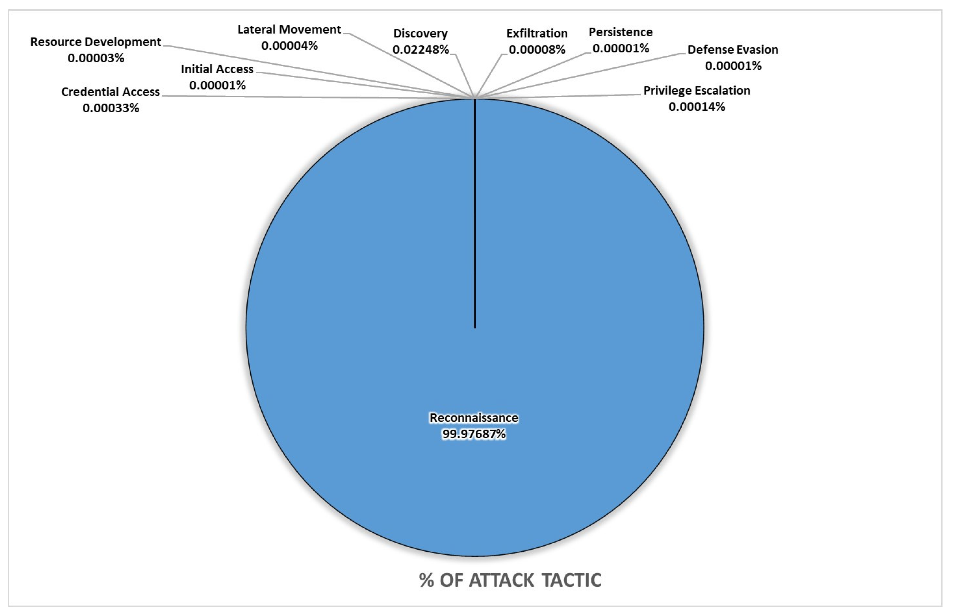
UWF-Zeekdata22 [10,11], a new dataset created in 2022, is a crowd-sourced dataset comprising benign as well as attack tactic data collected from Zeeklogs, an open-source network-monitoring tool used to collect data. This dataset, labeled using the MITRE Adversarial Tactics, Techniques, and Common Knowledge (ATT&CK) framework [32], has 9280 million tactic records and 9281 million benign records. The breakdown of the tactic data in UWF-ZeekData22 is presented in Figure 1. As can be seen from the dataset, the reconnaissance tactic makes up 99.97% of the attack tactics, and the second highest tactic is the discovery tactic, making up 0.02247%. The reconnaissance and discovery tactics were easily detectable using ML algorithms, as seen from [32]. These results will show that, though the discovery tactic made up a much smaller percentage of the dataset, this tactic was still detectable using ML algorithms without resampling.
The other tactics in this dataset, exfiltration lateral movement, resource development, credential access, privilege escalation, persistence, defense evasion, and initial access, have meager representation. These tactics are rare and would not be detectable using regular ML algorithms without resampling measures.
Out of the eight rare tactics in UWF-ZeekData22, in this study, we focused on only two rare tactics, privilege escalation, and credential access, which comprise 0.00014% and 0.00033% of the tactic data, respectively. These two tactics had the highest number of occurrences among the rare tactics in this dataset.
Privilege escalation is a tactic that refers to 14 different techniques that adversaries may use to obtain greater permissions in a system or network. This allows the adversary to access more resources and perform more actions that would have been impossible with their previous privileges; techniques involving exploiting software vulnerabilities or misconfigurations in the system, allowing them to gain higher-level privileges.
Credential access is a tactic that involves 17 different techniques that adversaries may use to obtain account credentials. These credentials can then access systems, applications, and sensitive information. Techniques for this tactic involve brute forcing, network sniffing, using credentials from dumping password stores, and even adversary-in-the-middle, where the attacker intercepts credentials.
5. The Experimental Setup
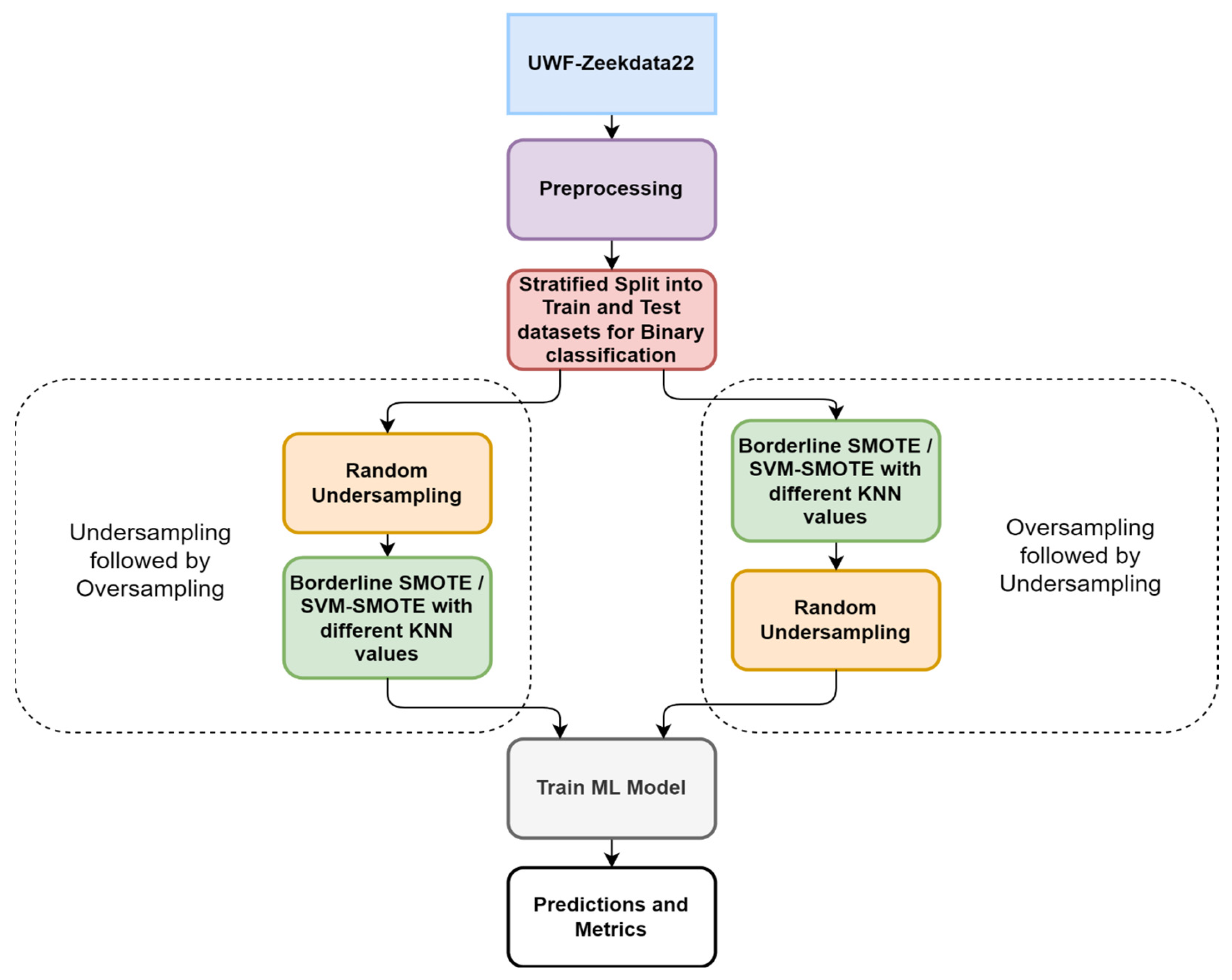
Figure 2 presents an overview of the experimental setup. As shown in Figure 2, the first step was to preprocess the data and then create training and testing datasets using stratified sampling; following this, the resampling was carried out. The ML model, random forest, was then trained on the resampled datasets, and the results were captured.
5.1. Preprocessing
Preprocessing followed [32], in which, first, the data were binned, and then the information gain [33] of the attributes was calculated.
After preprocessing, the training and testing datasets were created to perform binary classification. The first training and testing dataset was created with benign plus privilege escalation data and the second training and testing dataset was created with benign plus credential access data.
Stratified sampling was used to create these training and testing datasets. Stratified sampling was used to ensure that actual minority class instances were present in the trainingand testing datasets before performing synthetic generation using resampling techniques.
5.2. Approach to Resampling
Using the training and testing data, resampling was carried out using two approaches: (i) oversampling the minority data followed by undersampling, and (ii) undersampling the majority data followed by oversampling. These two approaches were compared in this study to analyze the order of resampling effectiveness.
Two oversampling techniques, BSMOTE and SVM-SMOTE, were used in both approaches, with RU of the majority class kept constant at 50% of the majority (benign) data. Oversampling ratios of 10% to 100% were used. Ten percent oversampling means the data were oversampled until 10% of the majority class was reached. Three values of KNN are selected for analysis—3, 5, and 8.
5.3. Machine Learning Model Used to Train Model
In this work, the random forest (RF) algorithm, initially proposed by Breiman [34] and a widely used ML algorithm, was used for classification. RF, which utilizes many decision trees to classify data, is less susceptive to overfitting and has gained its merit from its fast learning speed and high classification accuracy.
6. Metrics Used for Presentation of Results
In this section, we present the classification metrics as well as the Welch t-test results and analysis.
6.1. Classification Metrics Used
Accuracy, precision, recall, and macro-precision were used to evaluate the classification of the random forest results.
Accuracy is the number of correctly classified instances (i.e., true positives (TP) and negatives (TN)) divided by the total number of classifications [35].
Precision is the proportion of predicted positive cases correctly labeled positive [35]. Precision by label considers only one class and measures the number of times a specific label was predicted correctly, normalized by the number of times that label appears in the output.
where FP is the false positives.
Recall is the ability of the classifier to find all the positive samples or the true positive rate. Recall is also known as sensitivity and is the proportion of real positive cases that are correctly predicted as positive [35].
when FN is the false positives and TN is the true negatives.
F-Score is the harmonic mean of a prediction’s precision and recall metrics. It is another overall measure of the test’s accuracy [35].
Macro-precision is the arithmetic mean of each individual class’s precision.
6.2. Welch’s t-Tests
The final objective was to find the best classification results with the lowest oversampling ratios. Welch’s t-tests were used to compare two population means (in this case, the results of two oversampling ratios) with unequal variances. Because of unequal variances, the Satterthwaite approximation was used to obtain the degrees of freedom (d.f.).
7. Results and Discussion
This section presents the results of ML runs for binary classification using random forest. Binary classification means that data from each attack were separately combined with benign data.
Four sets of runs were performed for each minority class tactic, privilege escalation and credential access: (i) the first set of runs used data composed of oversampling using BSMOTE followed by undersampling; (ii) the second set of runs used data composed of undersampling followed by oversampling using BSMOTE; (iii) the third set of runs used data composed of oversampling using SVM-SMOTE followed by undersampling; (iv) and the fourth set of runs used data composed of undersampling followed by oversampling using SVM-SMOTE. And all results presented are an average of 10 runs.
KNN was varied for each set of runs and, for all processing, undersampling (without replacement) was limited to 50% of the majority class and oversampling was varied from 10% to 100% of the majority class. In all the datasets, the non-attack (benign) data was the majority class, and the particular tactic was the minority class. Each combination was run ten times and all results presented are an average of ten runs.
First, the BSMOTE oversampling followed by random undersampling results are presented using privilege escalation and credential access and then the SVM-SMOTE oversampling followed by random undersampling results are presented using privilege escalation and credential access. Then, the random undersampling followed by BSMOTE oversampling for privilege escalation and credential access followed by the corresponding SVM-SMOTE oversampling results are presented.
All the resulting metrics were analyzed using Welch’s t-tests. The means were compared. The first mean was compared to the second, and the better of the two results were compared with the next mean, and so on. The best results are highlighted in green. In some cases, when two paths were taken, the best results are highlighted in green as well as yellow. For brevity’s sake, all the tables have not been presented for Welch’s t-tests. Ater the first table showing the analysis for Privilege Escalation for BSMOTE oversampling using KNN = 3 followed by random undersamping, only the tables that had a divergence in the results were presented.
7.1. Selection of KNN
Since the SMOTE algorithms use KNN, the effect of varying KNN was studied. KNN = 3, 5, and 8 were used.
7.2. BSMOTE Oversampling Followed by Random Undersampling
This section presents the results for BSMOTE oversampling using varied KNN, followed by random undersampling. Using UWF-ZeekData22, we are considering two minority attack tactics, privilege escalation and credential access, which have 0.00007% and 0.00016% of tactic data, respectively [10,11].
7.2.1. Privilege Escalation: BSMOTE Oversampling with Varying KNN Followed by Random Undersampling
For KNN = 3, 0.1 BSMOTE oversampling gave better overall results, as shown in Table 1, and probabilistic analysis of the Welch’s t-test results shown in Table 2 found that 0.1 oversampling consistently had better precision, F-score, and macro-precision than higher oversampling percentages.
The average metric values for the KNN = 5 runs are presented in Table 3. Probabilistic analysis of the Welch’s t-test results found that the 0.3 BSMOTE oversampling ratio had better recall and F-score than the rest of the oversampling ratios. Welch’s t-test results also found no significant differences between the variations in precision and macro-precision.
Table 4 shows the metric values for KNN = 8. When 0.1 and 0.2 oversampling ratios were compared, as shown in Table 5 and Table 6, respectively, Welch’s t-test results showed that the former had better precision and macro-precision while the latter had a better recall. At this juncture a divergence was observed, and analysis was performed on the two courses possible—continuing the study with 0.1 and 0.2 separately. When continuing with 0.1, as shown in Table 5, it was observed that 0.5 had better recall than the former, and there were no statistical differences from the rest of the oversampling results. This result is highlighted in green color in Table 4. On the other hand, with 0.2, as shown in Table 6, it had a better F-score than 0.3 and 0.7 and better recall than 0.7 and 0.1. There were no statistical differences observed with the rest of the oversampling percentages. Hence, 0.2 is highlighted in yellow in Table 4.
7.2.2. Credential Access: BSMOTE Oversampling with Varying KNN Followed by Random Undersampling
In this section, credential access is oversampled using BSMOTE, with varying KNN, at the various oversampling percentages, and then benign data are undersampled to 0.5. Table 7 shows the average metric values for KNN = 3, highlighting the best result at 0.4 oversampling. Welch’s t-test calculations showed 0.2 had a better F-score than 0.1, but there were no statistical differences from 0.3, but 0.4 had better precision and macro-precision than 0.2, 0.8, and 0.9. No statistical differences were observed in the Welch’s t-test scores for the other percentages.
For KNN = 5, as shown in Table 8, the best oversampling percentage was 0.1. Welch’s t-test results showed that there were no statistical differences with oversampling percentages from 0.1 to 0.4 but had better recall and F-score than 0.5. Along with its precision and macro-precision values, 0.1 had better recall than 0.7. No other significant differences were found with the remaining oversampling percentages until 1.0.
Table 9 shows the best oversampling percentage as 0.4 for KNN = 8. The p-values calculated for the analysis of Welch’s t-test scores showed that, initially, 0.3 performed better than 0.1 in precision and macro-precision, but it was replaced by 0.4, which performed better than the former. There were no statistical differences from 0.5 to 0.8 and 0.1. Additionally, 0.4 also performed better than 0.9 in precision, F-score, and macro-precision.
7.3. SVM-SMOTE Oversampling Followed by Random Undersampling
This section varies SVM-SMOTE oversampling percentages with KNN = 3, 5, and 8 while keeping the RU constant at 0.5.
7.3.1. Privilege Escalation: SVM-SMOTE Oversampling with Varied KNN Followed by Random Undersampling
For KNN = 3, as shown in Table 10, 0.1 oversampling had better overall results. With Welch’s t-test, probabilistic value calculations showed that 0.1 had better recall and F-score than 0.2, 0.3, and 1.0. There were no statistical differences observed with 0.4, 0.5, and 0.7. Additionally, 0.1 was better than 0.9 across all metrics.
For KNN = 5, no statistical differences were observed between 0.1 and higher oversampling percentages, and thus, 0.1 was selected as the overall better-performing oversampling percentage, as shown in Table 11.
For KNN = 8, two oversampling percentages gave better results, as highlighted in yellow and green color in Table 12. As for the Welch’s t-test analysis, it was observed that 0.3 had better recall than 0.1, and it was selected for further analysis. As the analysis progressed, 0.5 had better precision, F-score, and macro-precision than 0.3, while the latter had a better recall. Since it was difficult to conclude which was better, 0.3 or 0.5, two branches of analysis were performed—one with 0.3 and the other with 0.5. The Welch’s t-test results with 0.3 are presented in Table 13 and the analysis with 0.5 is shown in Table 14. When 0.5 was chosen, 0.6 had better results than 0.5, with better recall, while 0.6 also had better precision, F-score, and macro-precision than 0.9 and 1.0. These results are presented in Table 12. On the other branch where 0.3 was selected, 0.3 showed no statistical difference from 0.4, 0.6, 0.7, 0.9, and 1.0. It had a better recall than 0.8.
7.3.2. Credential Access: SVM-SMOTE Oversampling with Varying KNN Followed by Random Undersampling
For credential access, for KNN = 3 (Table 15), 0.7 oversampling percentage gave better results than the other values. From initial p-value calculations, it appeared that 0.3 had better precision than 0.1 and better precision, F-score, and macro-precision than 0.4, and no statistical differences from 0.5 and 0.6 results. However, 0.7 had better recall than 0.1 and better precision, F-score, and macro-precision than 0.8 and 0.9. No statistical differences were observed between 0.7 and 1.0.
For KNN = 5 (Table 16), probabilistic calculations resulted in 0.1 having the overall best results. No statistical differences were present for lower oversampling percentages until 0.6. Additionally, 0.1 consistently had better recall, F-score, and macro-precision values than higher percentages from 0.7 to 1.0.
For KNN = 8, average metrics results are presented in Table 17. Welch’s t-test calculations showed that 0.3 consistently performed better than higher oversampling percentages. Hence, it was chosen as the best oversampling percentage for KNN = 8 credential access data with SVM-SMOTE executed first, followed by RU.
7.4. Random Undersampling Followed by BSMOTE Oversampling
In this section, RU to 0.5 was first performed on the majority class or benign data before oversampling using BSMOTE using different KNN values.
7.4.1. Privilege Escalation: Random Undersampling Followed by BSMOTE Oversampling with Varying KNN
For KNN = 3 (Table 18), probabilistic analysis of Welch’s t-tests resulted in 0.2 oversampling giving the best results. We found 0.2 had better recall and F-score than 0.1, 0.9, and 1.0, better recall than 0.4, 0.7, and 1.0. No statistical differences were observed with 0.3, 0.5, 0.6, and 0.8.
For KNN = 5 (Table 19), 0.1 had better recall than 0.4, and 0.5 oversampling was better than 0.1 across all metrics in Welch’s t-test calculations. We found 0.5 was better than other higher oversampling percentages until 0.9 and had no statistical differences from 1.0.
For KNN = 8 (Table 20), no statistical differences were observed between results 0.1, 0.2, and 0.3. When 0.1 was compared with 0.4, the former had better precision, F-score, and precision, while the latter had a better recall. A divergence was observed (see Table 21 and Table 22) where there was an option to proceed with 0.1 or 0.4. When 0.4 was taken as the successor (Table 21), 0.5 had a better recall than 0.4. While there were no statistical differences with 0.6, 0.7, 0.9, and 1.0, 0.5 had a better F-score than 0.8; hence, 0.5 was considered the best overall (highlighted in yellow in Table 20).
In the alternate scenario (Table 22), when 0.1 was taken for further comparisons, no statistical differences were observed with 0.5. However, 0.6 had a better F-score than 0.1. In the next comparison between 0.6 and 0.7, the latter had better recall; 0.7 had better recall than 0.8, and there were no statistical differences with the 0.9 results. Compared with 1.0, 0.7 had a better recall. However, 1.0 had better precision, F-score, and macro-precision than 0.7 (highlighted in green in Table 20).
7.4.2. Credential Access: Random Undersampling Followed by BSMOTE Oversampling with Varying KNN
This section presents an analysis of the credential access tactic with RU followed by BSMOTE oversampling with varying KNN results. Table 23 shows the results of runs with KNN = 3, where 0.5 BSMOTE oversampling gave better results in the probabilistic analysis. The Welch’s t-test results showed that, initially, 0.3 had better precision and macro-precision than 0.1, but 0.5 had even better precision, F-score, and macro-precision than the former. When compared with higher oversampling percentages, 0.5 had a better F-score than 0.6, precision, F-score, and macro-precision than 0.9 and 1.0.
For KNN = 5 (Table 24), 0.3 BSMOTE oversampling had better precision, F-score, and macro-precision than 0.1, 0.4, 0.5, 0.7, and 1.0. This is highlighted in green. Welch’s t-test results showed that the 0.3 oversampling ratio had no statistical difference between 0.3; it had better precision and macro-precision than 0.7 and 0.8.
For KNN = 8 (Table 25), p-value calculations revealed that 0.1 BSMOTE oversampling did not have any statistical difference from most of the higher oversampling percentages except for 0.7, where the former had better precision, F-score, and macro-precision. Hence, 0.1 was considered to give the best results, highlighted in green in Table 25.
7.5. Random Undersampling Followed by SVM-SMOTE Oversampling
In this analysis set, SVM-SMOTE using KNN 3, 5, and 8 was used for oversampling the minority classes for privilege escalation and credential access in the UWF-Zeekdata22 dataset.
7.5.1. Privilege Escalation: Random Undersampling Followed by SVM-SMOTE Oversampling with Varying KNN
For KNN = 3, Table 26 contains the average metrics values. Welch’s t-test results showed that 0.1 oversampling had better precision and macro-precision than 0.2, but 0.3 oversampling percentage had better recall than 0.1, 0.4, and 0.7. There were no statistical differences between the metrics of 0.3, 0.5, 0.6, and 0.9. Additionally, 0.3 had better recall and F-score than 0.8 and was better than 0.1 across all metrics; hence, 0.3 was selected as having the best overall results.
Table 27 shows the best oversampling ratio of 0.5 for KNN = 5. Welch’s t-test analysis showed that 0.1 SVM-SMOTE oversampling had better recall than 0.2 and better precision and macro-precision than 0.3 and 0.4. Therefore, 0.5 replaced 0.1 as the best overall percentage with better recall. No statistical differences existed with 0.6, 0.7, and 0.8 oversampling percentages. Additionally, 0.5 had better recall than 0.9 and 1.0 percentages; hence, 0.5 was selected as the best oversampling percentage.
The best overall percentage decreased to 0.2 for KNN = 8 (Table 28) for privilege escalation. Welch’s t-tests results showed that 0.2 oversampling had a better F-score than 0.1 but had no statistical differences from 0.3 and 0.4 values. It also had better F-scores than 0.5 and 0.6 and better recall than 0.7. However, 0.2, 0.8, and 0.9 were statistically identical; they had better recall than 1.0.
7.5.2. Credential Access: Random Undersampling Followed by SVM-SMOTE Oversampling with Varying KNN
Table 29 presents the results for RU of benign data followed by SVM-SMOTE oversampling using KNN = 3 of the minority tactic, credential access. When analyzing Welch’s t-test results, 0.2 had better recall than 0.1 and better recall and F-score than 0.3. However, it had no statistical differences from 0.4, 0.5, and 0.6. It had better precision and macro-precision than 0.7. However, though 0.2 followed the same pattern as 0.8, it has a better F-score. Though 0.2 has no significant differences from 0.9 and 1.0, it is chosen as the best-performing oversampling percentage since it has the least data.
For KNN = 5, as shown in Table 30, 0.1 SVM-SMOTE oversampling percentage gives better results than other values. When p-values were analyzed, 0.1 did not have statistically significant differences from the higher oversampling percentages except 0.5 and 0.8: 0.1 had better precision, F-score, and macro-precision than 0.5 and better recall and F-score than 0.8; hence, 0.1 was chosen as the best result.
For KNN = 8, 0.3 SVM-SMOTE oversampling gave better results than other ratios, as presented in Table 31. Welch’s t-test analysis showed that it had better recall and F-score than 0.1 and 0.4 and better recall than 0.5. For the higher oversampling percentages, 0.3 gave better precision and macro-precision than 0.7 and a better F-score than 0.8. It had no significant differences with the rest of the percentages; hence, 0.2 was selected as the best.
7.6. Summary of the Findings
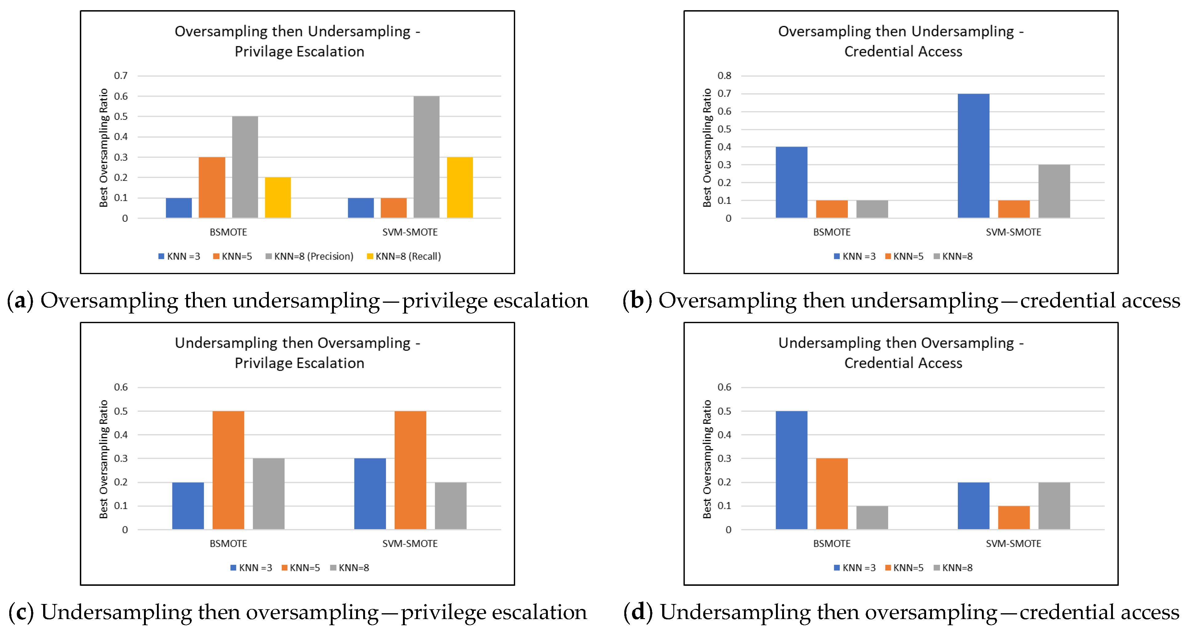
Figure 3 presents a summary of the findings. Figure 3a presents the best oversampling ratios for oversampling then undersampling for privilege escalation; Figure 3b presents the best oversampling ratios for oversampling then undersampling for credential access; Figure 3c presents the best oversampling ratios for undersampling then oversampling for privilege escalation; and Figure 3d presents the best oversampling ratios for undersampling then oversampling for credential access in UWF-Zeekdata22.
For BSMOTE for oversampling then undersampling for KNN = 8 for privilege escalation, precision was the best at the oversampling ratio of 0.5, but the recall was the best at the oversampling ratio of 0.2. For SVM-SMOTE, precision was the best at the oversampling ratio of 0.6, and recall was the best at recall of 0.3, as shown in Figure 3a.
7.7. Limitations of This Study
Since there were no other similar datasets available at the time of this work, this work was performed on only one dataset. This work needs to be tested on other similar datasets. Additionally, this dataset did not have enough data to test the other tactics.
8. Conclusions
This paper looks at the impact of the order of oversampling and undersampling on network attack tactic classification. From the results, it can be observed that the order of oversampling and undersampling matters; that is, it makes a difference whether we perform oversampling first or undersampling first. The results show that oversampling before undersampling provided better results. For oversampling before undersampling, for privilege escalation, BSMOTE and SVM-SMOTE performed equally well at a resampling ratio of 0.1, at KNN = 3. At KNN = 5, however, SVM-SMOTE performed better with a lower resampling ratio, but for KNN = 8, BSMOTE again had a lower resampling ratio. Of course, the final objective was to find the best classification results with the lowest oversampling ratios.
For credential access, however, BSMOTE used a lower resampling ratio for oversampling before undersampling.
For privilege escalation, KNN = 3 gave the best results with the lowest oversampling ratios, but for credential access, KNN = 5 gave the best results with the lowest oversampling ratios.
Contrary to the general notion, the data do not have to be oversampled to 50% (or the two sample sizes do not have to be even) to obtain the best results. In many cases, as have seen in our results, even oversampling of 10% of the minority data is enough.
These results conform to those of a previous work by Bagui et al. (2023) [16], so it can be concluded that 10% oversampling of minority data is enough for ML classification of attack data as well as tactic data. However, unlike with attack data, the order of resampling matters with tactic data.
9. Future Works
Future works will determine if these results have any practical implications. Another good study would to be test how these results compare when other oversampling techniques are used.
Author Contributions
Conceptualization S.S.B., D.M., S.C.B. and S.S.; methodology S.S.B., D.M., S.S.B. and S.S.; software S.S.; validation S.S.B., D.M., S.C.B. and S.S.; formal analysis S.S.B., D.M., S.C.B. and S.S.; investigation S.S.B., D.M., S.C.B. and S.S.; data curation S.S.; writing—original draft preparation S.S. and S.S.B; writing—review and editing S.S.B., D.M., S.C.B. and S.S.; visualization S.S.; supervision S.S.B., D.M. and S.C.B.; project administration S.S.B. and D.M.; funding acquisition S.S.B., D.M. and S.C.B. All authors have read and agreed to the published version of the manuscript.
Funding
This research was funded by the National Centers of Academic Excellence in Cybersecurity, 2021 NCAE-C-002: Cyber Research Innovation Grant Program, Grant Number: H98230-21-1-0170.
Data Availability Statement
The datasets are available at datasets.uwf.edu (accessed on 20 July 2023).
Acknowledgments
We would like to thank Mashall Elam for his assistance.
Conflicts of Interest
The authors declare no conflict of interest.
References
- Statista. Global Digital Population 2022. Available online: https://www.statista.com/statistics/617136/digital-population-worldwide/ (accessed on 3 August 2023).
- Cveticanin, N. Credit Card Fraud Statistics: What Are the Odds? Available online: https://dataprot.net/statistics/credit-card-fraud-statistics/ (accessed on 3 August 2023).
- CSIS. Significant Cyber Incidents. 2023. Available online: https://www.csis.org/programs/strategic-technologies-program/significant-cyber-incidents (accessed on 25 August 2023).
- Gottsegen, G. Machine Learning Cybersecurity: How It Works and Companies to Know. Available online: https://builtin.com/artificial-intelligence/machine-learning-cybersecurity (accessed on 25 August 2023).
- IBM. Cost of a Data Breach 2022. Available online: https://www.ibm.com/reports/data-breach (accessed on 25 August 2023).
- What Is the MITRE ATT&CK Framework? Get the 101 Guide. Trellix. 2022. Available online: https://www.trellix.com/en-us/security-awareness/cybersecurity/what-is-mitre-attack-framework.html (accessed on 25 August 2023).
- CrowdStrike. Machine Learning in Cybersecurity: Benefits and Use Cases. Available online: https://teams.microsoft.com/l/message/19:53e6bea1-e1f5-456a-abc7-a70b2fed5f46_abc83e5c-dd3c-45d8-a0e7-592e61673ca0@unq.gbl.spaces/1710410537020?context=%7B%22contextType%22%3A%22chat%22%7D (accessed on 25 August 2023).
- Mukherjee, B.; Heberlein, L.; Levitt, K.N. Network intrusion detection. IEEE Network 1994, 8, 26–41. [Google Scholar] [CrossRef]
- Bagui, S.; Li, K. Resampling Imbalanced Data for Network Intrusion Detection Datasets. J. Big Data 2021, 8, 6. [Google Scholar] [CrossRef]
- UWF-ZeekData22 Dataset. Available online: https://datasets.uwf.edu/ (accessed on 20 July 2023).
- Bagui, S.S.; Mink, D.; Bagui, S.C.; Ghosh, T.; Plenkers, R.; McElroy, T.; Dulaney, S.; Shabanali, S. Introducing UWF-ZeekData22: A Comprehensive Network Traffic Dataset Based on the MITRE ATT&CK Framework. Data 2023, 8, 18. [Google Scholar] [CrossRef]
- MITRE ATT&CK®. MITRE ATT&CK Reconnaissance, Tactic TA0043—Enterprise 2022. Available online: https://attack.mitre.org/tactics/TA0043/ (accessed on 25 August 2023).
- MITRE ATT&CK®. MITRE ATT&CK Discovery, Tactic TA0007—Enterprise 2022. Available online: https://attack.mitre.org/tactics/TA0007/ (accessed on 25 August 2023).
- Privilege Escalation. Available online: https://attack.mitre.org/tactics/TA0004/ (accessed on 25 August 2023).
- Credential Access. Available online: https://attack.mitre.org/tactics/TA0006/ (accessed on 25 August 2023).
- Bagui, S.S.; Mink, D.; Bagui, S.C.; Subramaniam, S. Determining Resampling Ratios Using BSOMTE and SVM-SMOTE for Identifying Rare Attacks in Imbalanced Cybersecurity Data. Computers 2023, 12, 204. [Google Scholar] [CrossRef]
- Krawczyk, B. Learning from imbalanced data: Open challenges and future directions. Prog. Artif. Intell. 2016, 5, 221–232. [Google Scholar] [CrossRef]
- Han, H.; Wang, W.; Mao, B. Borderline-SMOTE: A new Over-Sampling method in imbalanced Data sets learning. In Lecture Notes in Computer Science; Springer: Berlin/Heidelberg, Germany, 2005; pp. 878–887. [Google Scholar] [CrossRef]
- Kubát, M.; Matwin, S. Addressing the Curse of Imbalanced Training Sets: One-Sided selection. In Proceedings of the Fourteenth International Conference on Machine Learning (ICML 1997), Nashville, TN, USA, 8–12 July 1997; pp. 179–186. Available online: https://dblp.uni-trier.de/db/conf/icml/icml1997.html#KubatM97 (accessed on 25 August 2023).
- Nguyen, H.M.; Cooper, E.W.; Kamei, K. Borderline over-sampling for Imbalanced Data Classification. Int. J. Knowl. Eng. Soft Data Paradig. 2011, 3, 4. [Google Scholar] [CrossRef]
- Elreedy, D.; Atiya, A. A Comprehensive Analysis of Synthetic Minority Oversampling Technique (SMOTE) for Handling Class Imbalance. Inf. Sci. 2019, 505, 32–64. [Google Scholar] [CrossRef]
- Chawla, N.V.; Bowyer, K.W.; Hall, L.O.; Kegelmeyer, W.P. SMOTE: Synthetic Minority Over-sampling technique. J. Artif. Intell. Res. 2002, 16, 321–357. [Google Scholar] [CrossRef]
- Batista, G.E.; Prati, R.C.; Monard, M.C. A study of the behavior of several methods for balancing machine learning training data. SIGKDD Explor. 2004, 6, 20–29. [Google Scholar] [CrossRef]
- Fernández, A.; García, S.; Herrera, F.; Chawla, N.V. SMOTE for Learning from Imbalanced Data: Progress and Challenges, Marking the 15-year Anniversary. J. Artif. Intell. Res. 2018, 61, 863–905. [Google Scholar] [CrossRef]
- Tauscher, Z.; Jiang, Y.; Zhang, K.; Wang, J.; Song, H. Learning to Detect: A Data-driven Approach for Network Intrusion Detection. In Proceedings of the 2021 IEEE International Performance, Computing, and Communications Conference (IPCCC), Austin, TX, USA, 29–31 October 2021. [Google Scholar] [CrossRef]
- Liu, Z.; Han, Q.; Zhu, J. A combination method of resampling and random forest for imbalanced data classification. In Proceedings of the 4th International Conference on Advances in Computer Technology, Information Science and Communications (CTISC), Suzhou, China, 22–24 April 2022. [Google Scholar] [CrossRef]
- Chakravarthy, A.D.; Bonthu, S.; Chen, Z.; Zhu, Q. Predictive Models with Resampling: A Comparative Study of Machine Learning Algorithms and their Performances on Handling Imbalanced Datasets. In Proceedings of the 18th IEEE International Conference on Machine Learning and Applications (ICMLA), Boca Raton, FL, USA, 16–19 December 2019. [Google Scholar] [CrossRef]
- Douzas, G.; Bacao, F.; Last, F. Improving Imbalanced Learning through a Heuristic Oversampling Method based on K-means and SMOTE. Inf. Sci. 2018, 465, 1–20. [Google Scholar] [CrossRef]
- Wang, X.; Li, Y.; Zhange, J.; Zhang, B.; Gong, H. An Oversampling Method based on Differential Evolution and Natural Neighbors. Appl. Soft Comput. 2023, 149, 110952. [Google Scholar] [CrossRef]
- Li, M.; Zhou, H.; Liu, Q.; Gong, X.; Wang, G. A Weighted Oversampling Framework with Relative Neighborhood Density for Imbalanced Noisy Classification. Expert Syst. Appl. 2024, 241, 122593. [Google Scholar] [CrossRef]
- Joloudari, J.H.; Marefat, A.; Nenatollahi, M.A.; Oyelere, S.S.; Hussain, S. Effective Class-Imbalance Learning Based on SMOTE and Convolutional Neural Networks. Appl. Sci. 2023, 13, 4006. [Google Scholar] [CrossRef]
- Bagui, S.; Mink, D.; Bagui, S.; Ghosh, T.; McElroy, T.; Paredes, E.; Khasnavis, N.; Plenkers, R. Detecting Reconnaissance and Discovery Tactics from the MITRE ATT&CK Framework in Zeek Conn Logs Using Spark’s Machine Learning in the Big Data Framework 2018. Sensors 2022, 22, 7999. [Google Scholar] [CrossRef]
- Han, J.; Kamber, M.; Pei, J. Data Mining: Concepts and Techniques; Morgan Kaufmann: Cambridge, MA, USA, 2022. [Google Scholar]
- Breiman, L. Random Forests. Mach. Learn. 2001, 45, 5–32. [Google Scholar] [CrossRef]
- Powders David, M.W. Evaluation: From Precision, Recall and F-Measure to ROC, Informedness, Markedness & Correlation. J. Mach. Learn. Technol. 2011, 2, 37–63. [Google Scholar]

Figure 2.
Experimental design.

Figure 3.
Plot of best oversampling ratios.


Table 1.
Privilege escalation: BSMOTE oversampling using KNN = 3 followed by RU.
| Oversampling % | Accuracy | Precision | Recall | F-Score | Macro-Precision |
|---|---|---|---|---|---|
| 0.1 | 0.999 | 1.000 | 0.850 | 0.880 | 0.999 |
| 0.2 | 0.999 | 0.766 | 0.600 | 0.600 | 0.883 |
| 0.3 | 0.999 | 0.780 | 0.900 | 0.833 | 0.889 |
| 0.4 | 0.999 | 0.620 | 0.650 | 0.627 | 0.809 |
| 0.5 | 0.999 | 0.933 | 0.950 | 0.931 | 0.966 |
| 0.6 | 0.999 | 0.707 | 0.800 | 0.716 | 0.853 |
| 0.7 | 0.999 | 0.698 | 0.850 | 0.750 | 0.849 |
| 0.8 | 0.999 | 0.826 | 0.900 | 0.831 | 0.913 |
| 0.9 | 0.999 | 0.853 | 0.950 | 0.886 | 0.926 |
| 1.0 | 0.999 | 0.626 | 0.600 | 0.585 | 0.813 |
Table 2.
Welch’s t-test: privilege escalation: BSMOTE oversampling using KNN = 3 followed by RU.
| Welch’s t-Test (p < 0.10) | Precision t Value | Recall t Value | F-Score t Value | Macro-Precision t Value | Analysis |
|---|---|---|---|---|---|
| 0.1 vs. 0.2 | 2.608 | 1.234 | 2.013 | 2.608 | 0.1 has better precision, F-score, and macro-precision than 0.2 |
| 0.1 vs. 0.3 | 3.074 | −0.310 | 0.353 | 3.074 | 0.1 has better precision and macro-precision than 0.3 |
| 0.1 vs. 0.4 | 3.849 | 1.240 | 1.785 | 3.849 | 0.1 has better precision, F-score, and macro-precision than 0.4 |
| 0.1 vs. 0.5 | 1.118 | −0.707 | −0.451 | 1.118 | No statistical diffrerence between 0.1 and 0.5 |
| 0.1 vs. 0.6 | 3.685 | 0.288 | 1.335 | 3.685 | 0.1 has better precision and macro-precision than 0.6 |
| 0.1 vs. 0.7 | 3.302 | 0.000 | 0.962 | 3.302 | 0.1 has better precision and macro-precision than 0.7 |
| 0.1 vs. 0.8 | 2.589 | −0.310 | 0.413 | 2.589 | 0.1 has better precision and macro-precision than 0.8 |
| 0.1 vs. 0.9 | 2.536 | −0.707 | −0.062 | 2.536 | 0.1 has better precision and macro-precision than 0.9 |
| 0.1 vs. 1 | 2.482 | 1.165 | 1.672 | 2.482 | 0.1 has better precision, F-score, and macro-precision than 0.9 |
Table 3.
Privilege escalation: BSMOTE oversampling using KNN = 5 followed by RU.
| Oversampling % | Accuracy | Precision | Recall | F-Score | Macro-Precision |
|---|---|---|---|---|---|
| 0.1 | 0.999 | 0.866 | 0.900 | 0.853 | 0.933 |
| 0.2 | 0.999 | 0.693 | 0.900 | 0.777 | 0.846 |
| 0.3 | 0.999 | 0.933 | 1.000 | 0.960 | 0.966 |
| 0.4 | 0.999 | 0.845 | 0.850 | 0.820 | 0.922 |
| 0.5 | 0.999 | 0.866 | 0.800 | 0.807 | 0.933 |
| 0.6 | 0.999 | 0.706 | 0.750 | 0.682 | 0.853 |
| 0.7 | 0.999 | 0.866 | 0.800 | 0.828 | 0.933 |
| 0.8 | 0.999 | 0.793 | 0.750 | 0.758 | 0.896 |
| 0.9 | 0.999 | 0.700 | 0.550 | 0.580 | 0.849 |
| 1.0 | 0.999 | 0.920 | 0.750 | 0.768 | 0.959 |
Table 4.
Privilege escalation: BSMOTE oversampling using KNN = 8 followed by RU.
| Oversampling % | Accuracy | Precision | Recall | F-Score | Macro-Precision |
|---|---|---|---|---|---|
| 0.1 | 0.999 | 0.624 | 0.650 | 0.510 | 0.812 |
| 0.2 | 0.999 | 0.240 | 1.000 | 0.347 | 0.620 |
| 0.3 | 0.999 | 0.101 | 0.900 | 0.180 | 0.550 |
| 0.4 | 0.999 | 0.089 | 0.750 | 0.159 | 0.544 |
| 0.5 | 0.999 | 0.407 | 1.000 | 0.465 | 0.703 |
| 0.6 | 0.999 | 0.263 | 0.900 | 0.251 | 0.631 |
| 0.7 | 0.999 | 0.236 | 0.550 | 0.148 | 0.618 |
| 0.8 | 0.999 | 0.384 | 0.900 | 0.408 | 0.692 |
| 0.9 | 0.999 | 0.255 | 0.850 | 0.301 | 0.627 |
| 1.0 | 0.999 | 0.447 | 0.800 | 0.455 | 0.723 |
Table 5.
Welch’s t-test: privilege escalation: BSMOTE oversampling using KNN = 8 followed by RU.
| Welch’s t-Test (p < 0.10) | Precision t Value | Recall t Value | F-Score t Value | Macro- Precision t Value | Analysis |
|---|---|---|---|---|---|
| 0.1 vs. 0.2 | 1.696 | −2.608 | 0.869 | 1.696 | 0.1 has better precision and macro-precision than 0.2, except for recall, which is better in the latter. |
| 0.1 vs. 0.3 | 2.541 | −1.550 | 2.085 | 2.541 | 0.1 is better than 0.3 across all metrics except recall, where 0.3 performs better. |
| 0.1 vs. 0.4 | 2.592 | −0.512 | 2.192 | 2.592 | 0.1 has better precision, F-score, and macro-precision than 0.4. |
| 0.1 vs. 0.5 | 0.791 | −2.608 | 0.189 | 0.791 | 0.5 has better recall than 0.1. |
| 0.5 vs. 0.6 | 0.586 | 1.118 | 1.080 | 0.586 | No statistical difference between 0.5 and 0.6 |
| 0.5 vs. 0.7 | 0.683 | 2.515 | 1.709 | 0.683 | 0.5 has better recall and F-score than 0.7 |
| 0.5 vs. 0.8 | 0.092 | 1.118 | 0.248 | 0.092 | No statistical difference between 0.5 and 0.8 |
| 0.5 vs. 0.9 | 0.616 | 1.118 | 0.697 | 0.616 | No statistical difference between 0.5 and 0.9 |
| 0.5 vs. 1.0 | −0.161 | 1.825 | 0.047 | −0.161 | 0.5 has better recall than 1.0 |
Table 6.
Welch’s t-test: privilege escalation: BSMOTE oversampling using KNN = 8 followed by RU.
| Welch’s t-Test (p < 0.10) | Precision t Value | Recall t Value | F-Score t Value | Macro- Precision t Value | Analysis |
|---|---|---|---|---|---|
| 0.1 vs. 0.2 | 1.696 | −2.608 | 0.869 | 1.696 | 0.1 has better precision and macro-precision than 0.2, except for recall, which is better in the latter. |
| 0.2 vs. 0.3 | 1.432 | 1.118 | 1.593 | 1.432 | 0.2 has a better F-score than 0.3 |
| 0.2 vs. 0.4 | 1.538 | 1.767 | 1.747 | 1.538 | 0.2 is better than 0.4 across all metrics |
| 0.2 vs. 0.5 | −0.812 | 0.000 | −0.579 | −0.812 | No statistical difference between 0.2 and 0.5 |
| 0.2 vs. 0.6 | −0.122 | 1.118 | 0.700 | −0.122 | No statistical difference between 0.2 and 0.6 |
| 0.2 vs. 0.7 | 0.018 | 2.515 | 1.679 | 0.018 | 0.2 has better recall and F-score than 0.7 |
| 0.2 vs. 0.8 | −0.736 | 1.118 | −0.331 | −0.736 | No statistical difference between 0.2 and 0.8 |
| 0.2 vs. 0.9 | −0.078 | 1.118 | 0.248 | −0.078 | No statistical difference between 0.2 and 0.9 |
| 0.2 vs. 1.0 | −1.066 | 1.825 | −0.661 | −1.066 | 0.2 has better recall than 1.0 |
Table 7.
Credential access: BSMOTE oversampling using KNN = 3 followed by RU.
| Oversampling % | Accuracy | Precision | Recall | F-Score | Macro-Precision |
|---|---|---|---|---|---|
| 0.1 | 0.999 | 0.655 | 0.888 | 0.740 | 0.827 |
| 0.2 | 0.999 | 0.703 | 0.977 | 0.815 | 0.851 |
| 0.3 | 0.999 | 0.745 | 0.911 | 0.801 | 0.872 |
| 0.4 | 0.999 | 0.802 | 0.888 | 0.831 | 0.901 |
| 0.5 | 0.999 | 0.736 | 0.866 | 0.788 | 0.868 |
| 0.6 | 0.999 | 0.760 | 0.911 | 0.814 | 0.880 |
| 0.7 | 0.999 | 0.727 | 0.911 | 0.795 | 0.863 |
| 0.8 | 0.999 | 0.669 | 0.911 | 0.760 | 0.834 |
| 0.9 | 0.999 | 0.662 | 0.755 | 0.688 | 0.831 |
| 1.0 | 0.999 | 0.845 | 0.933 | 0.885 | 0.922 |
Table 8.
Credential access: BSMOTE oversampling using KNN = 5 followed by RU.
| Oversampling % | Accuracy | Precision | Recall | F-Score | Macro-Precision |
|---|---|---|---|---|---|
| 0.1 | 0.999 | 0.770 | 0.955 | 0.843 | 0.885 |
| 0.2 | 0.999 | 0.700 | 0.888 | 0.778 | 0.850 |
| 0.3 | 0.999 | 0.773 | 0.933 | 0.839 | 0.886 |
| 0.4 | 0.999 | 0.806 | 0.911 | 0.850 | 0.903 |
| 0.5 | 0.999 | 0.713 | 0.755 | 0.728 | 0.856 |
| 0.6 | 0.999 | 0.718 | 0.911 | 0.802 | 0.859 |
| 0.7 | 0.999 | 0.625 | 0.911 | 0.737 | 0.812 |
| 0.8 | 0.999 | 0.568 | 0.822 | 0.663 | 0.784 |
| 0.9 | 0.999 | 0.748 | 0.933 | 0.803 | 0.874 |
| 1.0 | 0.999 | 0.670 | 0.822 | 0.727 | 0.835 |
Table 9.
Credential access: BSMOTE oversampling using KNN = 8 followed by RU.
| Oversampling % | Accuracy | Precision | Recall | F-Score | Macro-Precision |
|---|---|---|---|---|---|
| 0.1 | 0.999 | 0.647 | 0.733 | 0.670 | 0.823 |
| 0.2 | 0.999 | 0.604 | 0.977 | 0.741 | 0.802 |
| 0.3 | 0.999 | 0.731 | 0.933 | 0.809 | 0.865 |
| 0.4 | 0.999 | 0.768 | 0.955 | 0.846 | 0.884 |
| 0.5 | 0.999 | 0.780 | 0.977 | 0.861 | 0.889 |
| 0.6 | 0.999 | 0.686 | 0.911 | 0.773 | 0.843 |
| 0.7 | 0.999 | 0.671 | 1.000 | 0.800 | 0.835 |
| 0.8 | 0.999 | 0.713 | 0.933 | 0.798 | 0.856 |
| 0.9 | 0.999 | 0.588 | 0.933 | 0.717 | 0.794 |
| 1.0 | 0.999 | 0.708 | 0.866 | 0.771 | 0.854 |
Table 10.
Privilege escalation: SVM-SMOTE oversampling using KNN = 3 followed by RU.
| Oversampling % | Accuracy | Precision | Recall | F-Score | Macro-Precision |
|---|---|---|---|---|---|
| 0.1 | 0.999 | 0.960 | 1.000 | 0.977 | 0.980 |
| 0.2 | 0.999 | 0.933 | 0.600 | 0.674 | 0.966 |
| 0.3 | 0.999 | 0.900 | 0.700 | 0.751 | 0.949 |
| 0.4 | 0.999 | 0.933 | 0.900 | 0.914 | 0.966 |
| 0.5 | 0.999 | 0.960 | 1.000 | 0.977 | 0.980 |
| 0.6 | 0.999 | 0.883 | 0.850 | 0.864 | 0.941 |
| 0.7 | 0.999 | 0.866 | 1.000 | 0.920 | 0.933 |
| 0.8 | 0.999 | 0.893 | 0.750 | 0.751 | 0.946 |
| 0.9 | 0.999 | 0.680 | 0.850 | 0.743 | 0.839 |
| 1.0 | 0.999 | 0.900 | 0.650 | 0.733 | 0.949 |
Table 11.
Privilege escalation: SVM-SMOTE oversampling using KNN = 5 followed by RU.
| Oversampling % | Accuracy | Precision | Recall | F-Score | Macro-Precision |
|---|---|---|---|---|---|
| 0.1 | 0.999 | 0.807 | 0.900 | 0.816 | 0.903 |
| 0.2 | 0.999 | 0.933 | 0.900 | 0.914 | 0.966 |
| 0.3 | 0.999 | 0.933 | 0.900 | 0.893 | 0.966 |
| 0.4 | 0.999 | 0.700 | 0.900 | 0.780 | 0.849 |
| 0.5 | 0.999 | 0.920 | 0.950 | 0.933 | 0.959 |
| 0.6 | 0.999 | 0.853 | 0.950 | 0.886 | 0.926 |
| 0.7 | 0.999 | 0.826 | 0.750 | 0.768 | 0.913 |
| 0.8 | 0.999 | 0.822 | 0.850 | 0.763 | 0.911 |
| 0.9 | 0.999 | 0.900 | 0.750 | 0.800 | 0.949 |
| 1.0 | 0.999 | 0.893 | 0.900 | 0.892 | 0.946 |
Table 12.
Privilege escalation: SVM-SMOTE oversampling using KNN = 8 followed by RU.
| Oversampling % | Accuracy | Precision | Recall | F-Score | Macro-Precision |
|---|---|---|---|---|---|
| 0.1 | 0.999 | 0.110 | 0.800 | 0.189 | 0.555 |
| 0.2 | 0.999 | 0.119 | 0.900 | 0.207 | 0.559 |
| 0.3 | 0.999 | 0.119 | 1.000 | 0.208 | 0.559 |
| 0.4 | 0.999 | 0.121 | 1.000 | 0.213 | 0.560 |
| 0.5 | 0.999 | 0.477 | 0.650 | 0.393 | 0.738 |
| 0.6 | 0.999 | 0.372 | 1.000 | 0.449 | 0.686 |
| 0.7 | 0.999 | 0.176 | 0.950 | 0.292 | 0.588 |
| 0.8 | 0.999 | 0.211 | 0.750 | 0.252 | 0.605 |
| 0.9 | 0.999 | 0.084 | 0.850 | 0.153 | 0.542 |
| 1.0 | 0.999 | 0.099 | 1.000 | 0.180 | 0.549 |
Table 13.
Welch’s t-test: privilege escalation: SVM-SMOTE oversampling using KNN = 8 followed by RU.
Table 13.
Welch’s t-test: privilege escalation: SVM-SMOTE oversampling using KNN = 8 followed by RU.
| Welch’s t-Test (p < 0.10) | Precision t Value | Recall t Value | F-Score t Value | Macro- Precision t Value | Analysis |
|---|---|---|---|---|---|
| 0.1 vs. 0.2 | −0.202 | −0.707 | −0.278 | −0.202 | No statistical difference between 0.1 and 0.2 |
| 0.1 vs. 0.3 | −0.207 | −1.825 | −0.301 | −0.207 | 0.3 has better recall than 0.1 |
| 0.3 vs. 0.4 | −0.065 | 0.000 | −0.095 | −0.065 | No statistical difference between 0.3 and 0.4 |
| 0.3 vs. 0.5 | −2.321 | 2.608 | −1.951 | −2.321 | 0.5 is better than 0.3 in precision, F-score and macro-precision. 0.3 has better recall than 0.5 |
| 0.5 vs. 0.6 | 0.470 | −2.608 | −0.312 | 0.470 | 0.6 has better recall than 0.5 |
| 0.6 vs. 0.7 | 1.181 | 1.118 | 0.960 | 1.181 | No statistical difference between 0.6 and 0.7 |
| 0.6 vs. 0.8 | 0.833 | 1.767 | 1.129 | 0.833 | 0.6 has better recall than 0.8 |
| 0.6 vs. 0.9 | 1.748 | 1.118 | 1.841 | 1.748 | 0.6 has better precision, F-score, and macro-precision than 0.9 |
| 0.6 vs. 1.0 | 1.667 | 0.000 | 1.700 | 1.667 | 0.6 has better precision, F-score, and macro-precision than 1.0 |
Table 14.
Welch’s t-test: privilege escalation: SVM-SMOTE oversampling using KNN = 8 followed by RU.
Table 14.
Welch’s t-test: privilege escalation: SVM-SMOTE oversampling using KNN = 8 followed by RU.
| Welch’s t-Test (p < 0.10) | Precision t Value | Recall t Value | F-Score t Value | Macro- Precision t Value | Analysis |
|---|---|---|---|---|---|
| 0.1 vs. 0.2 | −0.202 | −0.707 | −0.278 | −0.202 | No statistical difference between 0.1 and 0.2 |
| 0.1 vs. 0.3 | −0.207 | −1.825 | −0.301 | −0.207 | 0.3 has better recall than 0.1 |
| 0.3 vs. 0.4 | −0.065 | 0.000 | −0.095 | −0.065 | No statistical difference between 0.3 and 0.4 |
| 0.3 vs. 0.5 | −2.321 | 2.608 | −1.951 | −2.321 | 0.5 is better than 0.3 in precision, F-score, and macro-precision. 0.3 has better recall than 0.5 |
| 0.3 vs. 0.6 | −1.532 | 0.000 | −1.485 | −1.532 | No statistical difference between 0.3 and 0.6 |
| 0.3 vs. 0.7 | −1.475 | 1.118 | −1.423 | −1.475 | No statistical difference between 0.3 and 0.7 |
| 0.3 vs. 0.8 | −0.873 | 1.767 | −0.512 | −0.873 | 0.3 has better recall than 0.8 |
| 0.3 vs. 0.9 | 1.123 | 1.118 | 1.101 | 1.123 | No statistical difference between 0.3 and 0.9 |
| 0.3 vs. 1.0 | 0.740 | 0.000 | 0.673 | 0.740 | No statistical difference between 0.3 and 1.0 |
Table 15.
Credential access: SVM-SMOTE oversampling using KNN = 3 followed by RU.
| Oversampling % | Accuracy | Precision | Recall | F-Score | Macro-Precision |
|---|---|---|---|---|---|
| 0.1 | 0.999 | 0.657 | 0.888 | 0.752 | 0.828 |
| 0.2 | 0.999 | 0.663 | 0.844 | 0.739 | 0.831 |
| 0.3 | 0.999 | 0.815 | 0.888 | 0.846 | 0.907 |
| 0.4 | 0.999 | 0.633 | 0.866 | 0.717 | 0.816 |
| 0.5 | 0.999 | 0.701 | 0.866 | 0.764 | 0.850 |
| 0.6 | 0.999 | 0.697 | 0.955 | 0.798 | 0.848 |
| 0.7 | 0.999 | 0.775 | 1.000 | 0.859 | 0.887 |
| 0.8 | 0.999 | 0.629 | 0.888 | 0.727 | 0.814 |
| 0.9 | 0.999 | 0.619 | 0.844 | 0.709 | 0.809 |
| 1.0 | 0.999 | 0.698 | 0.955 | 0.803 | 0.849 |
Table 16.
Credential access: SVM-SMOTE oversampling using KNN = 5 followed by RU.
| Oversampling % | Accuracy | Precision | Recall | F-Score | Macro-Precision |
|---|---|---|---|---|---|
| 0.1 | 0.999 | 0.775 | 0.955 | 0.852 | 0.887 |
| 0.2 | 0.999 | 0.697 | 0.777 | 0.725 | 0.848 |
| 0.3 | 0.999 | 0.765 | 0.933 | 0.837 | 0.882 |
| 0.4 | 0.999 | 0.672 | 0.911 | 0.762 | 0.836 |
| 0.5 | 0.999 | 0.748 | 0.955 | 0.818 | 0.874 |
| 0.6 | 0.999 | 0.783 | 0.933 | 0.849 | 0.891 |
| 0.7 | 0.999 | 0.733 | 0.822 | 0.758 | 0.866 |
| 0.8 | 0.999 | 0.686 | 0.866 | 0.763 | 0.843 |
| 0.9 | 0.999 | 0.675 | 0.911 | 0.772 | 0.837 |
| 1.0 | 0.999 | 0.673 | 0.888 | 0.755 | 0.836 |
Table 17.
Credential access: SVM-SMOTE oversampling using KNN = 8 followed by RU.
| Oversampling % | Accuracy | Precision | Recall | F-Score | Macro-Precision |
|---|---|---|---|---|---|
| 0.1 | 0.999 | 0.709 | 0.888 | 0.784 | 0.854 |
| 0.2 | 0.999 | 0.731 | 0.866 | 0.790 | 0.865 |
| 0.3 | 0.999 | 0.838 | 0.955 | 0.882 | 0.919 |
| 0.4 | 0.999 | 0.662 | 0.977 | 0.784 | 0.831 |
| 0.5 | 0.999 | 0.641 | 0.866 | 0.731 | 0.820 |
| 0.6 | 0.999 | 0.724 | 0.955 | 0.822 | 0.862 |
| 0.7 | 0.999 | 0.891 | 0.933 | 0.904 | 0.945 |
| 0.8 | 0.999 | 0.778 | 0.888 | 0.808 | 0.889 |
| 0.9 | 0.999 | 0.753 | 0.955 | 0.835 | 0.876 |
| 1.0 | 0.999 | 0.634 | 0.955 | 0.760 | 0.817 |
Table 18.
Privilege escalation: RU followed by BSMOTE oversampling using KNN = 3.
| Oversampling % | Accuracy | Precision | Recall | F-Score | Macro-Precision |
|---|---|---|---|---|---|
| 0.1 | 0.999 | 0.866 | 0.750 | 0.733 | 0.933 |
| 0.2 | 0.999 | 0.910 | 0.950 | 0.927 | 0.954 |
| 0.3 | 0.999 | 0.808 | 0.850 | 0.793 | 0.904 |
| 0.4 | 0.999 | 0.750 | 0.650 | 0.683 | 0.874 |
| 0.5 | 0.999 | 0.960 | 0.900 | 0.911 | 0.979 |
| 0.6 | 0.999 | 0.960 | 0.800 | 0.844 | 0.979 |
| 0.7 | 0.999 | 0.900 | 0.650 | 0.733 | 0.949 |
| 0.8 | 0.999 | 0.733 | 0.700 | 0.714 | 0.866 |
| 0.9 | 0.999 | 0.893 | 0.800 | 0.804 | 0.946 |
| 1.0 | 0.999 | 0.920 | 0.600 | 0.648 | 0.959 |
Table 19.
Privilege escalation: RU followed by BSMOTE oversampling using KNN = 5.
| Oversampling % | Accuracy | Precision | Recall | F-Score | Macro-Precision |
|---|---|---|---|---|---|
| 0.1 | 0.999 | 0.870 | 0.750 | 0.772 | 0.934 |
| 0.2 | 0.999 | 0.914 | 0.900 | 0.878 | 0.957 |
| 0.3 | 0.999 | 0.900 | 0.800 | 0.833 | 0.949 |
| 0.4 | 0.999 | 0.920 | 0.900 | 0.888 | 0.959 |
| 0.5 | 1.000 | 1.000 | 1.000 | 1.000 | 1.000 |
| 0.6 | 0.999 | 0.933 | 0.750 | 0.794 | 0.966 |
| 0.7 | 0.999 | 0.920 | 0.950 | 0.926 | 0.959 |
| 0.8 | 0.999 | 0.780 | 0.900 | 0.833 | 0.889 |
| 0.9 | 0.999 | 0.733 | 0.450 | 0.527 | 0.866 |
| 1.0 | 0.999 | 0.960 | 1.000 | 0.977 | 0.980 |
Table 20.
Privilege escalation: RU followed by BSMOTE oversampling using KNN = 8.
| Oversampling % | Accuracy | Precision | Recall | F-Score | Macro-Precision |
|---|---|---|---|---|---|
| 0.1 | 0.999 | 0.078 | 0.900 | 0.142 | 0.539 |
| 0.2 | 0.999 | 0.101 | 1.000 | 0.181 | 0.550 |
| 0.3 | 0.999 | 0.069 | 0.850 | 0.127 | 0.534 |
| 0.4 | 0.999 | 0.392 | 0.650 | 0.300 | 0.696 |
| 0.5 | 0.999 | 0.212 | 0.900 | 0.300 | 0.606 |
| 0.6 | 0.999 | 0.216 | 0.850 | 0.260 | 0.608 |
| 0.7 | 0.999 | 0.106 | 1.000 | 0.188 | 0.553 |
| 0.8 | 0.999 | 0.066 | 0.900 | 0.123 | 0.533 |
| 0.9 | 0.999 | 0.116 | 0.900 | 0.194 | 0.558 |
| 1.0 | 0.999 | 0.509 | 0.800 | 0.448 | 0.754 |
Table 21.
Welch’s t-test: privilege escalation: RU followed by SVM-SMOTE oversampling using KNN = 8.
Table 21.
Welch’s t-test: privilege escalation: RU followed by SVM-SMOTE oversampling using KNN = 8.
| Welch’s t-Test (p < 0.10) | Precision t Value | Recall t Value | F-Score t Value | Macro- Precision t Value | Analysis |
|---|---|---|---|---|---|
| 0.1 vs. 0.2 | −1.162 | −1.118 | −1.181 | −1.162 | No statistical difference between 0.1 and 0.2 |
| 0.1 vs. 0.3 | 0.573 | 0.310 | 0.550 | 0.573 | No statistical difference between 0.1 and 0.3 |
| 0.1 vs. 0.4 | −1.873 | 1.550 | −2.112 | −1.873 | 0.4 has better precision, F-score, and macro-precision than 0.1, while the latter has better recall |
| 0.4 vs. 0.5 | 0.919 | −1.550 | −0.002 | 0.919 | 0.5 has better recall than 0.4 |
| 0.5 vs. 0.6 | −0.026 | 0.395 | 0.296 | −0.026 | No statistical difference between 0.5 and 0.6 |
| 0.5 vs. 0.7 | 1.017 | −1.118 | 0.950 | 1.017 | No statistical difference between 0.5 and 0.7 |
| 0.5 vs. 0.8 | 1.427 | 0.000 | 1.560 | 1.427 | 0.5 has a better F-score than 0.8 |
| 0.5 vs. 0.9 | 0.913 | 0.000 | 0.898 | 0.913 | No statistical difference between 0.5 and 0.9 |
| 0.5 vs. 1.0 | −1.435 | 0.707 | −1.044 | −1.435 | No statistical difference between 0.5 and 1.0 |
Table 22.
Welch’s t-test: privilege escalation: RU followed by SVM-SMOTE oversampling using KNN = 8.
Table 22.
Welch’s t-test: privilege escalation: RU followed by SVM-SMOTE oversampling using KNN = 8.
| Welch’s t-Test (p < 0.10) | Precision t Value | Recall t Value | F-Score t Value | Macro- Precision t Value | Analysis |
|---|---|---|---|---|---|
| 0.1 vs. 0.2 | −1.162 | −1.118 | −1.181 | −1.162 | No statistical difference between 0.1 and 0.2 |
| 0.1 vs. 0.3 | 0.573 | 0.310 | 0.550 | 0.573 | No statistical difference between 0.1 and 0.3 |
| 0.1 vs. 0.4 | −1.873 | 1.550 | −2.112 | −1.873 | 0.4 has better precision, F-score, and macro-precision than 0.1, while the latter has a better recall |
| 0.1 vs. 0.5 | −1.312 | 0.000 | −1.384 | −1.312 | No statistical difference between 0.1 and 0.5 |
| 0.1 vs. 0.6 | −1.353 | 0.395 | −1.593 | −1.353 | 0.6 has a better F-score than 0.1 |
| 0.6 vs. 0.7 | 1.057 | −1.677 | 0.903 | 1.057 | 0.7 has better recall than 0.6 |
| 0.7 vs. 0.8 | 1.638 | 1.118 | 1.680 | 1.638 | 0.7 has better recall than 0.8 |
| 0.7 vs. 0.9 | −0.310 | 1.118 | −0.138 | −0.310 | No statistical difference between 0.7 and 0.9 |
| 0.7 vs. 1.0 | −2.218 | 1.825 | −2.773 | −2.218 | 1.0 is better than 0.7 across all metrics |
Table 23.
Credential access: RU followed by BSMOTE oversampling using KNN = 3.
| Oversampling % | Accuracy | Precision | Recall | F-Score | Macro-Precision |
|---|---|---|---|---|---|
| 0.1 | 0.999 | 0.639 | 0.888 | 0.741 | 0.819 |
| 0.2 | 0.999 | 0.619 | 0.800 | 0.686 | 0.809 |
| 0.3 | 0.999 | 0.733 | 0.888 | 0.799 | 0.866 |
| 0.4 | 0.999 | 0.739 | 0.866 | 0.781 | 0.869 |
| 0.5 | 0.999 | 0.893 | 0.866 | 0.872 | 0.946 |
| 0.6 | 0.999 | 0.819 | 0.755 | 0.714 | 0.909 |
| 0.7 | 0.999 | 0.828 | 0.888 | 0.843 | 0.914 |
| 0.8 | 0.999 | 0.796 | 0.888 | 0.822 | 0.898 |
| 0.9 | 0.999 | 0.662 | 0.866 | 0.743 | 0.831 |
| 1.0 | 0.999 | 0.734 | 0.777 | 0.746 | 0.867 |
Table 24.
Credential access: RU followed by BSMOTE oversampling using KNN = 5.
| Oversampling % | Accuracy | Precision | Recall | F-Score | Macro-Precision |
|---|---|---|---|---|---|
| 0.1 | 0.999 | 0.657 | 0.822 | 0.728 | 0.828 |
| 0.2 | 0.999 | 0.756 | 0.955 | 0.837 | 0.878 |
| 0.3 | 0.999 | 0.938 | 0.822 | 0.862 | 0.969 |
| 0.4 | 0.999 | 0.676 | 0.844 | 0.740 | 0.838 |
| 0.5 | 0.999 | 0.677 | 0.911 | 0.769 | 0.838 |
| 0.6 | 0.999 | 0.836 | 0.911 | 0.860 | 0.918 |
| 0.7 | 0.999 | 0.690 | 0.844 | 0.756 | 0.844 |
| 0.8 | 0.999 | 0.730 | 0.933 | 0.815 | 0.865 |
| 0.9 | 0.999 | 0.758 | 0.888 | 0.801 | 0.879 |
| 1.0 | 0.999 | 0.792 | 0.755 | 0.766 | 0.896 |
Table 25.
Credential access: RU followed by BSMOTE oversampling using KNN = 8.
| Oversampling % | Accuracy | Precision | Recall | F-Score | Macro-Precision |
|---|---|---|---|---|---|
| 0.1 | 0.999 | 0.746 | 0.844 | 0.780 | 0.873 |
| 0.2 | 0.999 | 0.697 | 0.933 | 0.786 | 0.848 |
| 0.3 | 0.999 | 0.635 | 0.888 | 0.719 | 0.817 |
| 0.4 | 0.999 | 0.702 | 0.911 | 0.769 | 0.851 |
| 0.5 | 0.999 | 0.684 | 0.911 | 0.779 | 0.842 |
| 0.6 | 0.999 | 0.647 | 0.911 | 0.747 | 0.823 |
| 0.7 | 0.999 | 0.629 | 0.888 | 0.714 | 0.814 |
| 0.8 | 0.999 | 0.741 | 0.844 | 0.773 | 0.870 |
| 0.9 | 0.999 | 0.811 | 0.888 | 0.823 | 0.905 |
| 1.0 | 0.999 | 0.706 | 0.933 | 0.789 | 0.853 |
Table 26.
Privilege escalation: RU followed by SVM-SMOTE oversampling using KNN = 3.
| Oversampling % | Accuracy | Precision | Recall | F-Score | Macro-Precision |
|---|---|---|---|---|---|
| 0.1 | 0.999 | 0.870 | 0.800 | 0.816 | 0.934 |
| 0.2 | 0.999 | 0.568 | 0.750 | 0.637 | 0.784 |
| 0.3 | 0.999 | 0.788 | 1.000 | 0.868 | 0.894 |
| 0.4 | 0.999 | 0.733 | 0.700 | 0.706 | 0.866 |
| 0.5 | 0.999 | 0.920 | 1.000 | 0.955 | 0.960 |
| 0.6 | 0.999 | 0.826 | 0.900 | 0.852 | 0.913 |
| 0.7 | 0.999 | 0.933 | 0.800 | 0.847 | 0.966 |
| 0.8 | 0.999 | 0.826 | 0.700 | 0.718 | 0.913 |
| 0.9 | 0.999 | 0.800 | 0.900 | 0.834 | 0.899 |
| 1.0 | 0.999 | 0.514 | 0.500 | 0.488 | 0.757 |
Table 27.
Privilege escalation: RU followed by SVM-SMOTE oversampling using KNN = 5.
| Oversampling % | Accuracy | Precision | Recall | F-Score | Macro-Precision |
|---|---|---|---|---|---|
| 0.1 | 0.999 | 0.910 | 0.800 | 0.807 | 0.954 |
| 0.2 | 0.999 | 0.700 | 0.450 | 0.533 | 0.849 |
| 0.3 | 0.999 | 0.708 | 0.950 | 0.798 | 0.854 |
| 0.4 | 0.999 | 0.786 | 0.800 | 0.763 | 0.893 |
| 0.5 | 0.999 | 0.853 | 1.000 | 0.915 | 0.926 |
| 0.6 | 0.999 | 0.874 | 0.950 | 0.894 | 0.937 |
| 0.7 | 0.999 | 0.900 | 0.900 | 0.866 | 0.949 |
| 0.8 | 0.999 | 0.826 | 1.000 | 0.897 | 0.913 |
| 0.9 | 0.999 | 0.800 | 0.600 | 0.666 | 0.899 |
| 1.0 | 0.999 | 0.860 | 0.700 | 0.724 | 0.929 |
Table 28.
Privilege escalation: RU followed by SVM-SMOTE oversampling using KNN = 8.
| Oversampling % | Accuracy | Precision | Recall | F-Score | Macro-Precision |
|---|---|---|---|---|---|
| 0.1 | 0.999 | 0.079 | 0.850 | 0.142 | 0.539 |
| 0.2 | 0.999 | 0.303 | 1.000 | 0.378 | 0.651 |
| 0.3 | 0.999 | 0.088 | 0.850 | 0.159 | 0.544 |
| 0.4 | 0.999 | 0.137 | 1.000 | 0.237 | 0.568 |
| 0.5 | 0.999 | 0.095 | 0.800 | 0.167 | 0.547 |
| 0.6 | 0.999 | 0.302 | 0.650 | 0.248 | 0.651 |
| 0.7 | 0.999 | 0.081 | 1.000 | 0.149 | 0.540 |
| 0.8 | 0.999 | 0.093 | 1.000 | 0.170 | 0.546 |
| 0.9 | 0.999 | 0.221 | 0.900 | 0.270 | 0.610 |
| 1.0 | 0.999 | 0.175 | 0.750 | 0.233 | 0.587 |
Table 29.
Credential access: RU followed by SVM-SMOTE oversampling using KNN = 3.
| Oversampling % | Accuracy | Precision | Recall | F-score | Macro-Precision |
|---|---|---|---|---|---|
| 0.1 | 0.999 | 0.774 | 0.777 | 0.758 | 0.887 |
| 0.2 | 0.999 | 0.731 | 0.933 | 0.815 | 0.865 |
| 0.3 | 0.999 | 0.720 | 0.800 | 0.755 | 0.860 |
| 0.4 | 0.999 | 0.734 | 0.955 | 0.820 | 0.867 |
| 0.5 | 0.999 | 0.700 | 0.911 | 0.776 | 0.850 |
| 0.6 | 0.999 | 0.666 | 0.888 | 0.756 | 0.833 |
| 0.7 | 0.999 | 0.663 | 0.911 | 0.754 | 0.831 |
| 0.8 | 0.999 | 0.618 | 0.933 | 0.740 | 0.809 |
| 0.9 | 0.999 | 0.717 | 0.977 | 0.821 | 0.858 |
| 1.0 | 0.999 | 0.758 | 0.822 | 0.749 | 0.879 |
Table 30.
Credential access: RU followed by SVM-SMOTE oversampling using KNN = 5.
| Oversampling % | Accuracy | Precision | Recall | F-Score | Macro-Precision |
|---|---|---|---|---|---|
| 0.1 | 0.999 | 0.761 | 0.933 | 0.827 | 0.880 |
| 0.2 | 0.999 | 0.719 | 0.911 | 0.782 | 0.859 |
| 0.3 | 0.999 | 0.761 | 0.911 | 0.826 | 0.880 |
| 0.4 | 0.999 | 0.713 | 0.955 | 0.809 | 0.856 |
| 0.5 | 0.999 | 0.668 | 0.888 | 0.759 | 0.834 |
| 0.6 | 0.999 | 0.768 | 0.911 | 0.825 | 0.884 |
| 0.7 | 0.999 | 0.788 | 0.977 | 0.862 | 0.894 |
| 0.8 | 0.999 | 0.709 | 0.822 | 0.741 | 0.854 |
| 0.9 | 0.999 | 0.813 | 0.866 | 0.817 | 0.906 |
| 1.0 | 0.999 | 0.759 | 0.844 | 0.786 | 0.879 |
Table 31.
Credential access: RU followed by SVM-SMOTE oversampling using KNN = 8.
| Oversampling % | Accuracy | Precision | Recall | F-Score | Macro-Precision |
|---|---|---|---|---|---|
| 0.1 | 0.999 | 0.703 | 0.777 | 0.726 | 0.851 |
| 0.2 | 0.999 | 0.707 | 0.888 | 0.784 | 0.853 |
| 0.3 | 0.999 | 0.746 | 0.955 | 0.834 | 0.873 |
| 0.4 | 0.999 | 0.746 | 0.800 | 0.762 | 0.873 |
| 0.5 | 0.999 | 0.750 | 0.777 | 0.762 | 0.874 |
| 0.6 | 0.999 | 0.744 | 1.000 | 0.851 | 0.872 |
| 0.7 | 0.999 | 0.640 | 0.955 | 0.763 | 0.820 |
| 0.8 | 0.999 | 0.710 | 0.844 | 0.722 | 0.855 |
| 0.9 | 0.999 | 0.789 | 0.888 | 0.826 | 0.894 |
| 1.0 | 0.999 | 0.700 | 0.933 | 0.789 | 0.850 |
Disclaimer/Publisher’s Note: The statements, opinions and data contained in all publications are solely those of the individual author(s) and contributor(s) and not of MDPI and/or the editor(s). MDPI and/or the editor(s) disclaim responsibility for any injury to people or property resulting from any ideas, methods, instructions or products referred to in the content. |
© 2024 by the authors. Licensee MDPI, Basel, Switzerland. This article is an open access article distributed under the terms and conditions of the Creative Commons Attribution (CC BY) license (https://creativecommons.org/licenses/by/4.0/).
Share and Cite
MDPI and ACS Style
Bagui, S.S.; Mink, D.; Bagui, S.C.; Subramaniam, S. Resampling to Classify Rare Attack Tactics in UWF-ZeekData22. Knowledge 2024, 4, 96-119. https://doi.org/10.3390/knowledge4010006
AMA Style
Bagui SS, Mink D, Bagui SC, Subramaniam S. Resampling to Classify Rare Attack Tactics in UWF-ZeekData22. Knowledge. 2024; 4(1):96-119. https://doi.org/10.3390/knowledge4010006
Chicago/Turabian StyleBagui, Sikha S., Dustin Mink, Subhash C. Bagui, and Sakthivel Subramaniam. 2024. "Resampling to Classify Rare Attack Tactics in UWF-ZeekData22" Knowledge 4, no. 1: 96-119. https://doi.org/10.3390/knowledge4010006