Three-Dimensional Path Tracking of Over-Actuated AUVs Based on MPC and Variable Universe S-Plane Algorithms

Abstract

Autonomous Underwater Vehicles (AUVs) are widely used for the inspection of seabed pipelines. To address the issues of low trajectory tracking accuracy in AUV inspection processes due to uncertain ocean current disturbances, this paper designs a new dual-loop controller based on Model Predictive Control (MPC) and Variable Universe S-plane algorithms (S-VUD FLC, where VUD represents Variable Universe Discourse and FLC represents Fuzzy Logic Control) to achieve three-dimensional (3-D) trajectory tracking of an over-actuated AUV under uncertain ocean current disturbances. This paper uses MPC as the outer-loop position controller and S-VUD FLC as the inner-loop speed controller. The outer-loop controller generates desired speed instructions that are passed to the inner-loop speed controller, while the inner-loop speed controller generates control input and uses a direct logic thrust distribution method that approaches optimal energy consumption to distribute the thrust generated by the propellers to the over-actuated AUV, achieving closed-loop tracking of the entire trajectory. When designing the outer-loop MPC controller, the actual control input constraints of the system are considered, and control increments are introduced to reduce control model errors and the impact of uncertain external disturbances on the actual AUV model parameters. When designing the inner-loop S-VUD FLC, the strong robustness of the variable universe fuzzy controller and the easy construction characteristics of the S-plane algorithm are combined, and integral action is introduced to improve the system’s tracking accuracy. The stability of the outer loop controller is proven by the Lyapunov method, and the stability of the inner loop controller is verified by simulation. Finally, simulations show that the over-actuated AUV has fast tracking processes and high tracking result accuracy under uncertain ocean current disturbances, demonstrating the effectiveness of the designed dual-loop controller.

1. Introduction

With the continuous advancement and innovation of autonomous navigation, control technology, sensor technology, communication technology, and energy technology, AUVs are capable of performing tasks in various complex underwater environments and are widely applied in ocean survey and research, marine resource exploration, and subsea pipeline and cable inspections [1]. The application of AUVs has increased the persistence and continuity of underwater monitoring and improved the autonomy and flexibility of underwater operations while reducing economic costs and avoiding potential personal injuries and losses [2]. Over-actuated AUVs, with more actuators and control inputs, have higher maneuverability and control capabilities compared to under-actuated AUVs, expanding the mission capabilities and application scope of AUVs. To ensure over-actuated AUVs can safely, stably, and accurately complete various underwater special tasks rapidly, further research on 3-D trajectory tracking control technology is required [3]. However, the model of over-actuated AUVs exhibits nonlinearity, coupling effects, and dynamic modeling complexity and is more sensitive to uncertainties such as modeling errors, environmental changes, and actuator failures [4]. These characteristics make the design and analysis of controllers for over-actuated AUVs more complex. Therefore, robust and precise control of over-actuated AUVs is crucial [5]. The direction of three-dimensional trajectory tracking control of autonomous underwater robots has always been a hot topic of keen interest [6].

So far, numerous classical control methods have been proposed by scholars worldwide for the 3-D trajectory tracking of underwater vehicles [7,8]. Examples include PID control, fuzzy control, backstepping control, sliding mode control (SMC), adaptive control, MPC, etc. The conventional PID control strategy often fails to achieve the desired control effect and is thus frequently combined with other control approaches to improve performance. Ye Li et al. combined an adaptive fuzzy algorithm with PID control to ensure that the AUV achieved accurate tracking of straight trajectories within a certain accuracy range [9]. However, due to the frequent variations in the model parameters of underwater vehicles caused by external environmental influences and frequent reference trajectory switching, the tuning of PID parameters becomes excessively complex and control performance remains unsatisfactory. By combining the Lyapunov method with backstepping control, virtual control quantities can be recursively constructed based on Lyapunov functions, which simplifies the design of complex control systems step by step [10]. Liang X et al. combined the backstepping method with sliding mode control to design a controller that utilized yaw angle as the input for tracking the horizontal path of an underactuated AUV [11]. Bing Huang et al. achieved controller synchronization through command-filtered backstepping design and a minimum learning parameter algorithm. They used a mapping function to transform the constrained control problem into an unconstrained one, demonstrating the superiority and effectiveness of this method through Lyapunov functions and simulations [12]. Nevertheless, as the order of the system increases, the introduction of virtual control quantities leads to a rapid increase in computational complexity, and the backstepping approach requires the establishment of accurate system models. Sliding mode control, by introducing sliding surfaces and sliding control laws, maintains good control performance even in the presence of parameter variations and external disturbances [13]. However, the chattering issue caused by the control input generated by the switching function in sliding mode control results in decreased control accuracy and reduces the lifespan of thrusters with long-term usage [14].

MPC can effectively handle the multi-degree-of-freedom control problem of over-actuated AUVs while fully considering the model and constraint conditions of the AUV, such as speed, torque, etc. [15]. It calculates the optimal control input in real time based on the system state and objective function in each control cycle, adjusting the control sequence to optimize tracking performance to the greatest extent and allowing the AUV to accurately follow the desired trajectory [16]. Moreover, MPC can also deal with the coupled dynamic effects in over-actuated AUVs, reduce the mutual interference between different degrees of freedom, and improve control performance [17]. Therefore, MPC has been widely used in the 3-D trajectory tracking of AUVs. Xuliang Yao et al. utilized MPC to derive the optimal guidance law and applied SMC for dynamic controller design. Their combination was shown, through simulations, to enhance the tracking performance of under-actuated AUVs following 3-D linear paths [18]. Yongding Zhang et al. proposed a three-dimensional trajectory tracking method based on MPC taking into account practical constraints. Simulations demonstrated that it can track grid scanning paths and sinusoidal curves [19]. Weiran Wang et al. simplified the kinematic model of the AUV into a five-degree-of-freedom (5-DOF) model and combined the Laguerre function and adaptive MPC, with simulations showing that it can achieve tracking of 3-D trajectories under disturbances while reducing computational complexity, though a dynamic controller was not designed [20]. Zheping Yan et al. used MPC to design a dual-loop controller, passed the speed commands generated by the outer-loop MPC to the inner-loop MPC, and performed simulation verification to show that the designed controller can track 3-D trajectories under external disturbances, though the design process of the inner-loop MPC was relatively complex [21].

Although the above studies adopt different control ideas, they have a common basic research idea, namely, to design trajectory tracking controllers by combining MPC with other control methods. A single MPC control algorithm cannot achieve tracking of 3-D trajectories [22]. S-VUD FLC is a combination of the classical S-plane control algorithm and the variable universe fuzzy method [23]. In variable universe fuzzy controllers, the introduction of a scaling universe part provides excellent robustness and adaptability, making the design of fuzzy controllers easier [24,25,26]. Compared with linear conventional PD control, the classical S-plane control algorithm with a nonlinear control surface is more suitable for the motion control of autonomous underwater robots [27]. Many scholars continue to deepen the demonstration and improvement of the S-plane control method and successfully apply it to various types of autonomous underwater robots [28,29]. The use of the S-plane to replace the fuzzy logic part in variable universe fuzzy controllers forms a new algorithm: the Variable Universe Discourse S-plane Controller (S-VUD FLC). The new algorithm combines the strong robustness of variable universe fuzzy controllers and the easy-to-construct characteristics of the S-plane algorithm, further simplifying controller design [30].

This paper thoroughly analyzes the trajectory tracking control problem of underwater vehicles, combines MPC with S-VUD FLC, and designs a new dual-loop controller based on MPC and S-VUD FLC. In order to improve the system’s robustness and adaptability, MPC is used as the outer-loop position controller and S-VUD FLC as the inner-loop speed controller. The speed control output of the outer-loop MPC controller is used as the desired control input for the inner-loop S-VUD FLC controller, ensuring accurate tracking of time-varying trajectories. To ensure smooth operation of the AUV when designing an MPC controller based on the kinematics model of the AUV, control increment input is introduced, and the actual control input constraints of the entire system are fully considered, i.e., the change range of linear speed and angular speed. The 3-D trajectory tracking problem is transformed into a standard quadratic programming (QP) problem with constraints. When the AUV moves to a new position, it calculates the optimal input of the inner-loop controller according to the current state and expectation. Meanwhile, when designing an S-VUD FLC controller based on the dynamics model of the AUV, the idea of the PID controller is borrowed, and the integral action is introduced to improve the tracking accuracy of the system, thus enhancing the system’s anti-interference ability against uncertain waves. To simulate a more realistic over-actuated AUV model and increase the control accuracy of the system, the mathematical model of the over-actuated AUV’s propeller is established. The direct logical thrust allocation method is used to distribute the thrust generated by the propeller to the over-actuated AUV in a way that is close to the optimal energy consumption. In the marine environment with complex interference effects, the over-actuated AUV can still complete the 3-D path target tracking task well. To verify the effectiveness of the designed dual-loop controller, the results of 3-D curve tracking simulations are provided, and the results prove the effectiveness of the designed controller.

The remainder of this paper is organized as follows: Section 2 presents the AUV model, the modeling of the propulsion system, and thrust allocation. Section 3 details the overall structure of the AUV’s 3-D trajectory tracking control based on MPC and P-S-VUD FLC, as well as proof of the stability of the kinematic controller. Section 4 validates the effectiveness of the designed controller through simulation. Finally, Section 5 concludes the paper.

2. Establishment of the “SZ-1” AUV Model

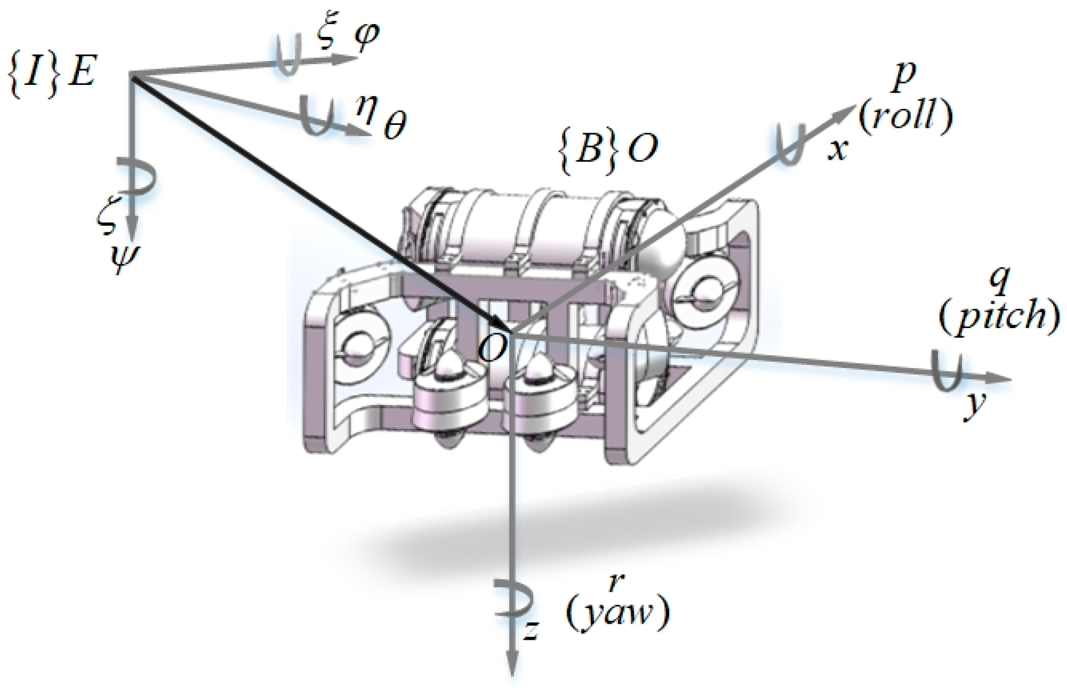
The over-actuated AUV studied in this paper is the “SZ-1” AUV, which was independently developed by China University of Petroleum (Beijing). The “SZ-1” AUV relies on four thrusters arranged in a vector layout on the horizontal plane and four thrusters on the vertical plane to achieve its six degrees of freedom attitude control. The motion and force analysis of the “SZ-1” AUV use two coordinate systems: the body coordinate system $\left\{B\right\}:O-xyz$ and the inertial coordinate system $\left\{I\right\}:E-\xi \eta \zeta$, where both adhere to the right-hand rule. The positive directions are respectively north, east, and downward [31]. The representation of “SZ-1” AUV in two coordinate systems is shown in Figure 1 below.

2.1. The Kinematic Model of the “SZ-1” AUV

In order to better describe the kinematics model of the AUV using mathematical language, let ${\eta }_1={\left[x,y,z\right]}^T$ and ${\eta }_2={\left[\phi ,\theta ,\psi \right]}^T$, representing the position and attitude in the inertial coordinate system, respectively. Let $\phi$ represent the pitch angle, $\theta$ represent the roll angle, and $\psi$ represent the heading angle. Let $V_1={\left[u,v,w\right]}^T$ and $V_2={\left[p,q,r\right]}^T$, representing the linear velocity and angular velocity in the body coordinate system, respectively. Finally, let $\eta ={\left[{{\eta }_1}^T,{{\eta }_2}^T\right]}^T$$={\left[x,y,z,\phi ,\theta ,\psi \right]}^T$.

The kinematic model of the over-actuated AUV is as follows:

$$\dot{\eta }=J(\eta )V=\left[\begin{array}{cc}{J}_1({\eta }_2)& 0_{3\times 3}\\ 0_{3\times 3}& J_2({\eta }_2)\end{array}\right]V$$

(1)

where

$${\dot{\eta }}_1=J_1({\eta }_2)V_1$$

(2)

$$J_1({\eta }_2)=\left[\begin{array}{ccc}\cos \theta \cos \psi & -\cos \phi \sin \psi +\sin \phi \sin \theta \cos \psi & \sin \phi \sin \psi +\cos \phi \sin \theta \cos \psi \\ \cos \theta \sin \psi & -\cos \phi \cos \psi +\sin \phi \sin \theta \sin \psi & -\sin \phi \cos \psi +\cos \phi \sin \theta \sin \psi \\ -\sin \theta & \cos \theta \sin \psi & \cos \phi \sin \theta \end{array}\right]$$

(3)

$${\dot{\eta }}_2=J_2({\eta }_2)V_2$$

(4)

$$J_2({\eta }_2)=\left[\begin{array}{ccc}1& \sin \phi \tan \theta & \cos \phi \tan \theta \\ 0& \cos \phi & -\sin \phi \\ 0& \frac{\sin \phi }{\cos \theta }& \frac{\cos \phi }{\cos \theta }\end{array}\right]$$

(5)

where $J(\eta )$ represents the transformation matrix between the body coordinate system and the inertial coordinate system, $0_{3\times 3}$ is a $3\times 3$ zero matrix, $J_1({\eta }_2)$ is the linear velocity transformation matrix, and $J_2({\eta }_2)$ is the angular velocity transformation matrix.

2.2. The Dynamic Model of the “SZ-1” AUV

The over-actuated AUV’s dynamic model based on the Newton–Euler method is

$$M\dot{V}+C(V)V+D(V)V+\mathrm{g}(\eta )=\tau +{\tau }_E$$

(6)

The explanations of each term in Equation (6) are as follows:

(1) $M$ is the inertia matrix, composed of the rigid body mass inertia matrix $M_{RB}$ and the added mass matrix $M_A$. The rigid body mass inertia matrix $M_{RB}$ represents the distribution of mass and the moment of inertia about the center of mass during the motion of the AUV. The added mass matrix $M_A$ represents the response of the added mass moments due to the fluid environment that the AUV encounters during its motion [32].

$$M=M_{RB}+M_A$$

(7)

where

$$M_{RB}={M_{RB}}^T=\left[\begin{array}{cccccc}m& 0& 0& 0& m{z}_g& m{y}_g\\ 0& m& 0& -m{z}_g& 0& m{x}_g\\ 0& 0& m& m{y}_g& -m{x}_g& 0\\ 0& -m{z}_g& m{y}_g& I_x& -I_{xy}& -I_{xz}\\ m{z}_g& 0& -m{x}_g& -I_{yx}& I_y& -I_{yz}\\ m{y}_g& m{x}_g& 0& -I_{zx}& -I_{zy}& I_z\end{array}\right]$$

(8)

$$M_A=\left[\begin{array}{cccccc}{X}_{\dot{u}}& X_{\dot{v}}& X_{\dot{w}}& X_{\dot{p}}& X_{\dot{q}}& X_{\dot{r}}\\ Y_{\dot{u}}& Y_{\dot{v}}& Y_{\dot{w}}& Y_{\dot{p}}& Y_{\dot{q}}& Y_{\dot{r}}\\ Z_{\dot{u}}& Z_{\dot{v}}& Z_{\dot{w}}& Z_{\dot{p}}& Z_{\dot{q}}& Z_{\dot{r}}\\ K_{\dot{u}}& K_{\dot{v}}& K_{\dot{w}}& K_{\dot{p}}& K_{\dot{q}}& K_{\dot{r}}\\ M_{\dot{u}}& M_{\dot{v}}& M_{\dot{w}}& M_{\dot{p}}& M_{\dot{q}}& M_{\dot{r}}\\ N_{\dot{u}}& N_{\dot{v}}& N_{\dot{w}}& N_{\dot{p}}& N_{\dot{q}}& N_{\dot{r}}\end{array}\right]$$

(9)

In Equations (8) and (9), $m$ represents the mass of the over-actuated AUV; $I_x$, $I_y$, $I_z$ represents the rotational inertia of the over-actuated AUV around its coordinate axes in the body frame; and $x_g$, $y_g$, $z_g$ represents the components of the center of gravity coordinates in the body frame. All terms in $M_A$ are first-order hydrodynamic derivatives, which characterize the added mass effects generated by the AUV’s motion in the fluid environment.

(2) $C(V)$ represents the Coriolis–centripetal moment matrix of the AUV, composed of the centripetal moment matrix $C_A(V)$ and the Coriolis moment matrix $C_{RB}(V)$. The centripetal moment matrix represents the effect of centripetal moments due to angular velocity during the AUV’s rotational motion. The Coriolis moment matrix $C_{RB}(V)$ describes the relationship between Coriolis forces, Coriolis moments, and the linear and angular velocities of the AUV. These forces do not actually act on the underwater vehicle but are used to explain the motion behavior of the AUV observed in a non-inertial reference frame [33].

$$C(V)=C_A(V)+C_{RB}(V)$$

(10)

where

$$C_A(V)=\left[\begin{array}{cccccc}0& 0& 0& 0& -a_3& a_2\\ 0& 0& 0& a_3& 0& -a_1\\ 0& 0& 0& -a_2& a_1& 0\\ 0& -a_3& a_2& 0& -b_3& b_2\\ a_3& 0& -a_1& b_3& 0& -b_1\\ -a_2& a_1& 0& -b_2& b_1& 0\end{array}\right]$$

(11)

$$C_{RB}(V)=\left[\begin{array}{cccccc}0& 0& 0& m(y_{g}q+z_{g}r)& -m(x_{g}q-w)& -m(x_{g}r-v)\\ 0& 0& 0& -m(y_{g}q+w)& m(z_{g}r+x_{g}p)& -m(y_{g}r-u)\\ 0& 0& 0& -m(z_{g}p-v)& -m(z_{g}q+u)& m(x_{g}p+y_{g}q)\\ -m(y_{g}q+z_{g}r)& m(y_{g}q+w)& m(z_{g}p-v)& 0& I_{z}r& I_{y}q\\ m(x_{g}q-w)& -m(z_{g}r+x_{g}p)& m(z_{g}q+u)& -I_{z}r& 0& I_{x}p\\ m(x_{g}r-v)& m(y_{g}r-u)& -m(x_{g}p+y_{g}q)& -I_{y}q& -I_{x}p& 0\end{array}\right]$$

(12)

In Equation (11), $a_1=X_{\dot{u}}u+X_{\dot{v}}v+X_{\dot{w}}w+X_{\dot{p}}p+X_{\dot{q}}q+X_{\dot{r}}r$,

$a_2=X_{\dot{v}}u+Y_{\dot{v}}v+Y_{\dot{w}}w+Y_{\dot{p}}p+Y_{\dot{q}}q+Y_{\dot{r}}r$, $a_3=X_{\dot{w}}u+Y_{\dot{w}}v+Z_{\dot{w}}w+Z_{\dot{p}}p+Z_{\dot{q}}q+Z_{\dot{r}}r$,

$b_1=X_{\dot{p}}u+Y_{\dot{p}}v+Z_{\dot{p}}w+K_{\dot{p}}p+K_{\dot{q}}q+K_{\dot{r}}r$, $b_2=X_{\dot{q}}u+Y_{\dot{q}}v+Z_{\dot{q}}w+K_{\dot{q}}p+M_{\dot{q}}q+M_{\dot{r}}r$,

$b_3=X_{\dot{r}}u+Y_{\dot{r}}v+Z_{\dot{r}}w+K_{\dot{r}}p+M_{\dot{r}}q+N_{\dot{r}}r$.

(3) $D(V)$ represents the fluid damping force and moment acting on the AUV during underwater motion. It is used to simulate the damping effect on the AUV caused by the viscosity and resistance of the fluid during its motion in the fluid, including water friction, wave damping, etc. [34].

$$D(V)=diag\left\{D_L+D_Q\left|V\right|\right\}$$

(13)

where $D_L$ represents the linear term and $D_Q$ represents the quadratic damping term.

$$D(V)=\left[\begin{array}{cccccc}{X}_u+X_{u\left|u\right|}\left|u\right|& 0& 0& 0& 0& 0\\ 0& Y_v+Y_{v\left|v\right|}\left|v\right|& 0& 0& 0& 0\\ 0& 0& Z_w+Z_{w\left|w\right|}\left|w\right|& 0& 0& 0\\ 0& 0& 0& K_p+K_{p\left|p\right|}\left|p\right|& 0& 0\\ 0& 0& 0& 0& M_q+M_{q\left|q\right|}\left|q\right|& 0\\ 0& 0& 0& 0& 0& N_r+N_{r\left|r\right|}\left|r\right|\end{array}\right]$$

(14)

In Equation (13), $X_u,Y_v,Z_w,K_p,M_q,N_r$ represent the first-order hydrodynamic coefficients of the AUV, and $X_{u\left|u\right|}\left|u\right|,Y_{v\left|v\right|}\left|v\right|,Z_{w\left|w\right|}\left|w\right|$,$K_{p\left|p\right|}\left|p\right|,M_{q\left|q\right|}\left|q\right|,N_{r\left|r\right|}\left|r\right|$ represent the second-order hydrodynamic coefficients of the AUV, indicating the nonlinear hydrodynamic effects when the AUV moves in the fluid. These coefficients are determined by the geometric shape of the AUV, the properties of the fluid, and the motion state of the AUV.

(4) $g(\eta )$ represents the matrix composed of the restorative forces and torques resulting from the effects of gravity and buoyancy.

$$g(\eta )=\left[\begin{array}{c}(W-B)\sin \theta \\ -(W-B)\sin \phi \cos \theta \\ -(W-B)\cos \phi \cos \theta \\ -\left(y_{g}W-y_{b}B\right)\cos \phi \cos \theta +\left(z_{g}W-x_{b}B\right)\sin \phi \cos \theta \\ \left(z_{g}W-z_{b}B\right)\sin \theta +\left(x_{g}W-x_{b}B\right)\cos \phi \cos \theta \\ -\left(x_{g}W-x_{b}B\right)\cos \phi \cos \theta -\left(y_{g}W-y_{b}B\right)\sin \theta \end{array}\right]$$

(15)

where $B$ represents the buoyancy generated by the AUV and $W$ represents the gravitational force acting on the AUV.

(5) $\tau$ represents the forces and torques generated on the AUV due to the combined action of eight propellers.

$$\tau ={\left[X,Y,Z,K,M,N\right]}^T$$

(16)

(6) ${\tau }_E$ represents the disturbances to the AUV due to its own model vibration and external interferences during operations.

$${\tau }_E={\left[d_u,d_v,d_w,d_p,d_q,d_r\right]}^T$$

(17)

2.3. Modelling and Thrust Allocation of the “SZ-1” AUV Propulsion System

Due to the nonlinearity, coupling effects, and complexity of dynamic modeling in the “SZ-1” AUV, it is more sensitive to uncertainties such as modeling errors, environmental changes, and actuator failures. The actuators of the “SZ-1” AUV consist of eight thrusters arranged in space. Therefore, we establish the mathematical models of its horizontal and vertical propulsion systems and analyze the spatial thrust distribution of the thrusters, making the modeling more refined and more in line with the actual physical model while discussing the thrust distribution methods [35].

2.3.1. Mathematical Modeling of the Horizontal and Vertical Propulsion Systems

The “SZ-1” AUV uses propeller thrusters produced by a certain manufacturer, with the control method being PWM. The direction and speed of rotation can be controlled by changing the input PWM duty cycle of the propeller thrusters. The relationship between thruster output force and propeller speed is as follows [36]:

$$T(n)=K_T\rho n^2{D}^4$$

(18)

In Equation (18), $T$ is the thrust generated by the propeller driven by the impeller, $N$; $K_T$ is the thrust coefficient of the propeller; $\rho$ is the density of seawater, $kg/m^3$; $n$ is the rotational speed of the propeller, $\mathrm{r}/\mathrm{s}$; and $D$ is the diameter of the propeller, $\mathrm{m}$. The maximum rotational speed is $n_{\max }=50$ $\mathrm{r}/\mathrm{s}$, $K_T=0.4$, $\rho =998.2$ $\mathrm{kg}/{\mathrm{m}}^3$, and $D=110$ $\mathrm{mm}$.

Table 1. Installation position and angle parameters of the AUV vector thrusters on “SZ-1”.

Number	Description	$\mathit{x}(\mathit{m})$	$\mathit{y}(\mathit{m})$	$\mathit{z}(\mathit{m})$	Installation Angle
$1$	Horizontal Bow Left	$c$	$-b$	$m$	Forms a 45° angle with the $Ox$-axis
$2$	Horizontal Bow Right	$c$	$b$	$m$	Forms a 45° angle with the $Ox$-axis
$3$	Horizontal Bow Left	$-c$	$-b$	$m$	Forms a 45° angle with the $Ox$-axis
$4$	Horizontal Bow Right	$-c$	$b$	$m$	Forms a 45° angle with the $Ox$-axis
$5$	Vertical Bow Left	$d$	$-f$	$n$	Perpendicular to the $xOy$ plane
$6$	Vertical Bow Right	$d$	$f$	$n$	Perpendicular to the $xOy$ plane
$7$	Vertical Bow Left	$-d$	$-f$	$n$	Perpendicular to the $xOy$ plane
$8$	Vertical Bow Right	$-d$	$f$	$n$	Perpendicular to the $xOy$ plane

where $c=0.3,b=0.2,d=0.1,f=0.1,m=0.1,n=-0.2$.

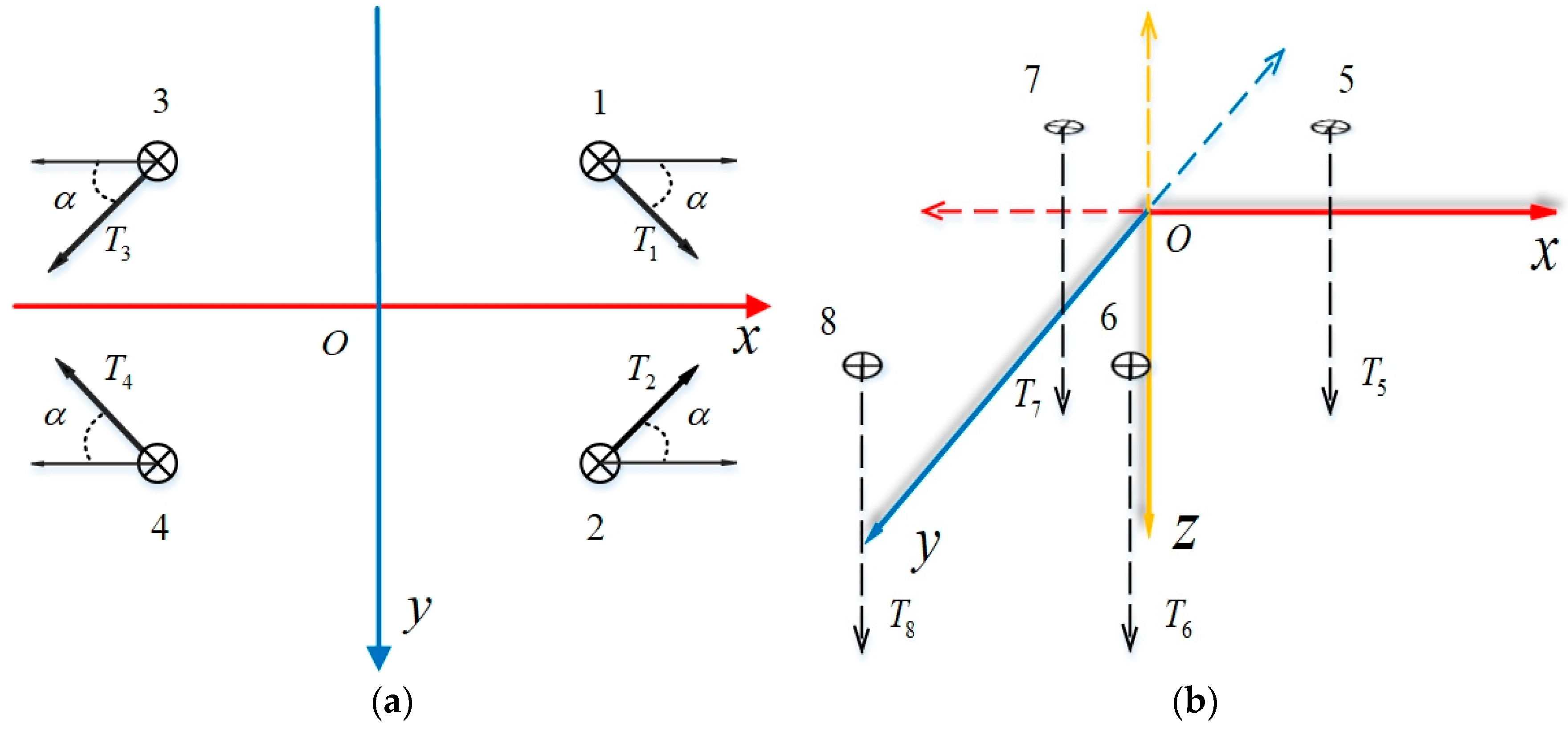
shows the installation positions and angles of the eight vectored thrusters of the “SZ-1” AUV in the body coordinate system. As can be seen from the table, the eight vectored thrusters are symmetrically installed. Since the horizontal thrusters are vectored, they can generate lateral motion.

Figure 2 shows the spatial layout of the thrusters on the “SZ-1” AUV. By analyzing the layout and thrust distribution of the eight vectored thrusters of the “SZ-1” AUV in the body coordinate system $\left\{B\right\}$, the expression of the force situation of the AUV in the six degrees of freedom is derived:

$$\{\begin{array}{l}X=(T_1+T_2+T_3+T_4)\cos \alpha \\ Y=(T_1-T_2-T_3+T_4)\sin \alpha \\ Z=T_5+T_6+T_7+T_8\\ K=f(-T_5+T_6-T_7+T_8)\\ M=d(-T_5-T_6+T_7+T_8)\\ N=c(T_1-T_2+T_3-T_4)\sin \alpha +b(T_1-T_2+T_3-T_4)\cos \alpha \end{array}$$

(19)

where $T_1$, $T_2$, $T_3$, and $T_4$ respectively represent the thrust exerted on the “SZ-1” AUV by the horizontal thrusters numbered 1, 2, 3, and 4, with all thrust directions forming an angle of 45° with the $Ox$ axis; $T_5$, $T_6$, $T_7$, and $T_8$ respectively represent the thrust exerted on the “SZ-1” AUV by the vertical thrusters numbered 5, 6, 7, and 8, with all thrust directions being perpendicular to the $Oz$ axis, forming an angle of 90°.

Consequently, the relationship between the thrust and torque vector matrix $\tau$ experienced by the “SZ-1” AUV and the thrust and torque generated by the eight thrusters can be further deduced as follows:

$$\tau =B{u}_c$$

(20)

where $\tau =\left[X,Y,Z,K,M,N\right]$, $u_c=\left[T_1,T_2,T_3,T_4,T_5,T_6,T_7,T_8\right]$, and $B$ represent the spatial vector arrangement matrix of the thrusters.

From Equation (20), the thruster vector arrangement matrix $B$ of the “SZ-1” AUV can be expressed as:

$$B=\left[\begin{array}{cccccccc}\cos \alpha & \cos \alpha & \cos \alpha & \cos \alpha & 0& 0& 0& 0\\ \sin \alpha & -\sin \alpha & -\sin \alpha & \sin \alpha & 0& 0& 0& 0\\ 0& 0& 0& 0& 1& 1& 1& 1\\ 0& 0& 0& 0& -f& f& -f& f\\ 0& 0& 0& 0& -d& -d& d& d\\ c\sin \alpha +b\cos \alpha & -c\sin \alpha -b\cos \alpha & c\sin \alpha +b\cos \alpha & -c\sin \alpha -b\cos \alpha & 0& 0& 0& 0\end{array}\right]$$

(21)

After accurate mathematical modeling of the horizontal and vertical propulsion systems is complete, the thrust distribution scheme can be discussed.

2.3.2. Thrust Allocation Method

The thrusters on the over-actuated AUV act as actuators, and the mathematical model of propulsion is the relationship between rotation speed and thrust. The thrust generated by the eight thrusters directly affects the AUV, causing changes in position and attitude. The direct logic distribution method is a thrust allocation method that closely approaches optimal energy consumption, having distinct advantages such as intuitiveness, simplicity, high efficiency, and strong real-time performance [37]. Therefore, we use the direct logic thrust allocation method to allocate the expected rotation speed for each thruster; the controller is responsible for outputting the expected input on each degree of freedom. The direct logic thrust allocation method converts the expected input into the expected rotation speed of each of the eight thrusters. By changing the PWM duty cycle on the microcontroller pin, the rotation direction and speed of the eight thrusters on the over-actuated AUV are controlled. Finally, according to the spatial arrangement of the thrusters on the over-actuated AUV, the thrust generated by the eight thrusters is applied to the AUV, thereby achieving the six-degrees-of-freedom movement of the over-actuated AUV.

(1)

Direct Logic Thrust Allocation Method for Horizontal Movement

The principle of the direct logic thrust allocation method for horizontal movement is as follows. All four thrusters in the horizontal plane rotating in the same direction can implement the forward and backward movements of the over-actuated AUV. Thrusters 1 and 4 rotate in the same direction, while thrusters 2 and 3 rotate in the opposite direction to implement the rightward movement of the over-actuated AUV. Similarly, by reversing the rotation directions of the four horizontal thrusters, the over-actuated AUV can move left. By keeping the speed of thrusters 1 and 2 unchanged and reversing the rotation direction of thrusters 3 and 4, the over-actuated AUV can perform left and right turns. These concepts can be expressed in the following equations:

$$\{\begin{array}{l}{T}_{d1}\left(n\right)=X_c\left(n\right)+Y_c\left(n\right)+N_c\left(n\right)\\ T_{d2}\left(n\right)=X_c\left(n\right)-Y_c\left(n\right)+N_c\left(n\right)\\ T_{d3}\left(n\right)=X_c\left(n\right)-Y_c\left(n\right)+N_c\left(n\right)\\ T_{d4}\left(n\right)=X_c\left(n\right)+Y_c\left(n\right)-N_c\left(n\right)\end{array}$$

(22)

where $X_c\left(n\right)$, $Y_c\left(n\right)$, and $N_c\left(n\right)$ are the expected inputs related to horizontal motion generated by the controller and $T_{d1}\left(n\right)$, $T_{d2}\left(n\right)$, $T_{d3}\left(n\right)$, and $T_{d4}\left(n\right)$ are the expected rotation speeds of the four thrusters in the horizontal plane, numbered 1, 2, 3, and 4, respectively.

(2)

Direct Logic Thrust Allocation Method for Vertical Movement

The principle of the direct logic thrust allocation method for vertical movement is as follows. All four thrusters in the vertical plane rotating in the same direction can implement the diving and surfacing movements of the over-actuated AUV. Thrusters 5 and 7 rotate in the opposite direction, while thrusters 6 and 8 rotate in the same direction to implement the anticlockwise rolling movement of the over-actuated AUV. Similarly, by reversing the rotation directions of the four vertical thrusters, the over-actuated AUV can perform a clockwise roll. Thrusters 5 and 6 rotate in the opposite direction while thrusters 7 and 8 rotate in the same direction to implement the downward pitching motion of the over-actuated AUV. Similarly, by reversing the rotation directions of the four vertical thrusters, the over-actuated AUV can perform an upward pitch. These concepts can be written in the following expressions:

$$\{\begin{array}{l}{T}_{d5}\left(n\right)=Z_c\left(n\right)-K_c\left(n\right)-M_c\left(n\right)\\ T_{d6}\left(n\right)=Z_c\left(n\right)+K_c\left(n\right)-M_c\left(n\right)\\ T_{d7}\left(n\right)=Z_c\left(n\right)-K_c\left(n\right)+M_c\left(n\right)\\ T_{d8}\left(n\right)=Z_c\left(n\right)+K_c\left(n\right)+M_c\left(n\right)\end{array}$$

(23)

where $Z_c\left(n\right)$, $K_c\left(n\right)$, and $M_c\left(n\right)$ are the expected rotational speed inputs related to vertical movement generated by the controller and $T_{d5}\left(n\right)$, $T_{d6}\left(n\right)$, $T_{d7}\left(n\right)$, and $T_{d8}\left(n\right)$ are the expected rotation speeds of the four thrusters in the vertical plane, numbered 5, 6, 7, and 8, respectively.

3. Establishment of Three-Dimensional Path Tracking Control Model

The AUV studied in this paper first needs to establish a 3-D path tracking control model, which includes an outer-loop kinematic control model and an inner-loop dynamic control model, and then design their respective controllers based on this foundation.

(1)

Outer-Loop Kinematic Control Model

Given that the “SZ-1” AUV is large and has a high center of buoyancy, the change in roll angle is relatively small when subjected to external force disturbances, indicating that the roll motion is self-stabilizing and can usually be ignored. To simplify the calculations, let the roll angle $\phi =0$ and the roll angular velocity $p=0$. Thus, the state vector in the inertial coordinate system can be simplified to $\eta ={\left[x,y,z,\theta ,\psi \right]}^T$, and the state vector in the body coordinate system can be simplified to $V={\left[u,v,w,q,r\right]}^T$. The relationship between the inertial coordinate system and the body coordinate system is then transformed as follows:

$$\dot{\eta }=J(\eta )V$$

(24)

where $\dot{\eta }={[\dot{x},\dot{y},\dot{z},\dot{\theta },\dot{\psi }]}^T$, $J(\eta )=\left[\begin{array}{ccccc}\cos \theta \cos \psi & -\sin \psi & \sin \theta \cos \psi & 0& 0\\ \cos \theta \sin \psi & \cos \psi & \sin \theta \sin \psi & 0& 0\\ -\sin \theta & 0& \cos \theta & 0& 0\\ 0& 0& 0& 1& 0\\ 0& 0& 0& 0& \frac{1}{\cos \theta }\end{array}\right]$

To obtain the kinematic control model, Equation (24) needs to be linearized. Let point $({\eta }_0,V_0)$ be its specific working point and perform Taylor expansion at point $({\eta }_0,V_0)$ to obtain the linearized equation (neglecting higher-order terms):

$$\dot{\eta }=J({\eta }_0)V_0+\frac{\mathsf{\partial }J(\eta )V}{\mathsf{\partial }\eta }{|}_{\begin{array}{l}\eta ={\eta }_0\\ V=V_0\end{array}}(\eta -{\eta }_0)+\frac{\mathsf{\partial }J(\eta )V}{\mathsf{\partial }V}{|}_{\begin{array}{l}\eta ={\eta }_0\\ V=V_0\end{array}}(\eta -V_0)$$

(25)

where $\frac{\mathsf{\partial }J(\eta )V}{\mathsf{\partial }\eta }{|}_{\begin{array}{l}\eta ={\eta }_0\\ V=V_0\end{array}}$ and $\frac{\mathsf{\partial }J(\eta )V}{\mathsf{\partial }V}{|}_{\begin{array}{l}\eta ={\eta }_0\\ V=V_0\end{array}}$ are 5 × 5 Jacobian matrices.

According to the kinematic equation shown in Equation (24), the expression of the specific working point $({\eta }_0,V_0)$ can be obtained:

$${\dot{\eta }}_0=J({\eta }_0)V_0$$

(26)

Subtracting Equation (26) from Equation (25) provides:

$$\begin{array}{l}\dot{\tilde{\eta }}=\left[\begin{array}{c}\dot{x}-{\dot{x}}_0\\ \dot{y}-{\dot{y}}_0\\ \dot{z}-{\dot{z}}_0\\ \dot{\theta }-{\dot{\theta }}_0\\ \dot{\psi }-{\dot{\psi }}_0\end{array}\right]=a\tilde{\eta }+\mathrm{b}\tilde{v}=\left[\begin{array}{ccccc}0& 0& 0& a_{14}& a_{15}\\ 0& 0& 0& a_{24}& a_{25}\\ 0& 0& 0& a_{34}& 0\\ 0& 0& 0& 0& 0\\ 0& 0& 0& 0& 0\end{array}\right]\left[\begin{array}{c}x-x_0\\ y-y_0\\ z-z_0\\ \theta -{\theta }_0\\ \psi -{\psi }_0\end{array}\right]\\ +\left[\begin{array}{ccccc}{b}_{11}& b_{12}& b_{13}& 0& 0\\ b_{21}& b_{22}& b_{23}& 0& 0\\ b_{31}& 0& b_{33}& 0& 0\\ 0& 0& 0& 1& 0\\ 0& 0& 0& 0& b_{55}\end{array}\right]\left[\begin{array}{c}u-u_0\\ v-v_0\\ w-w_0\\ q-q_0\\ r-r_0\end{array}\right]\end{array}$$

(27)

where $a_{14}=-u_0\sin {\theta }_0\cos {\psi }_0+w_0\cos {\theta }_0\cos {\psi }_0$, $a_{24}=-u_0\sin {\theta }_0\sin {\psi }_0+w_0\cos {\theta }_0\sin {\psi }_0$, $a_{34}=-u_0\cos {\theta }_0-w_0\sin {\theta }_0$, $a_{15}=-u_0\cos {\theta }_0\sin {\psi }_0-v_0\cos {\psi }_0-w_0\sin {\theta }_0\sin {\psi }_0$,

$a_{25}=u_0\cos {\theta }_0\cos {\psi }_0-v_0\sin {\psi }_0+w_0\sin {\theta }_0\cos {\psi }_0$, $b_{11}=\cos {\theta }_0\cos {\psi }_0$, $b_{12}=-\sin {\psi }_0$,

$b_{13}=\sin {\theta }_0\cos {\psi }_0$, $b_{21}=\cos {\theta }_0\sin {\psi }_0$, $b_{22}=\cos {\psi }_0$, $b_{23}=\sin {\theta }_0\sin {\psi }_0$, $b_{31}=-\sin {\theta }_0$, $b_{33}=\cos {\theta }_0$,

$b_{55}=\frac{1}{\cos {\theta }_0}$.

Equation (27) is the linear error kinematic control model for AUV 3-D path tracking, in which the model parameters are time-varying.

(2)

Inner-Loop Dynamic Control Model

Since the “SZ-1” AUV is designed with three sides of the shape being symmetrical to each other, some parameters in the dynamic model can be simplified to discard some non-essential items. Assuming that the change in the center of mass is not large and that it is right at the origin of the motion coordinate system, with the center of gravity set as the origin, the parameters of the simplified over-actuated AUV dynamics model are as follows:

$$M_{RB}=\left[\begin{array}{cccccc}m& 0& 0& 0& 0& 0\\ 0& m& 0& 0& 0& 0\\ 0& 0& m& 0& 0& 0\\ 0& 0& 0& I_x& 0& 0\\ 0& 0& 0& 0& I_y& 0\\ 0& 0& 0& 0& 0& I_z\end{array}\right]$$

(28)

$$M_A=\left[\begin{array}{cccccc}{X}_{\dot{u}}& 0& 0& 0& 0& 0\\ 0& Y_{\dot{v}}& 0& 0& 0& 0\\ 0& 0& Z_{\dot{w}}& 0& 0& 0\\ 0& 0& 0& K_{\dot{p}}& 0& 0\\ 0& 0& 0& 0& M_{\dot{q}}& 0\\ 0& 0& 0& 0& 0& N_{\dot{r}}\end{array}\right]$$

(29)

$$C_A(V)=\left[\begin{array}{cccccc}0& 0& 0& 0& -Z_{\dot{\mathrm{w}}}& Y_{\dot{\mathrm{v}}}v\\ 0& 0& 0& Z_{\dot{w}}& 0& -X_{\dot{u}}u\\ 0& 0& 0& -Y_{\dot{v}}& X_{\dot{u}}u& 0\\ 0& -Z_{\dot{w}}& Y_{\dot{v}}& 0& -N_{\dot{r}}r& M_{\dot{q}}q\\ Z_{\dot{w}}& 0& -X_{\dot{u}}u& N_{\dot{r}}r& 0& -K_{\dot{p}}p\\ -Y_{\dot{v}}& X_{\dot{u}}u& 0& -M_{\dot{q}}q& K_{\dot{p}}p& 0\end{array}\right]$$

(30)

$$D(V)=\left[\begin{array}{cccccc}{X}_u+X_{u\left|u\right|}\left|u\right|& 0& 0& 0& 0& 0\\ 0& Y_v+Y_{v\left|v\right|}\left|v\right|& 0& 0& 0& 0\\ 0& 0& Z_w+Z_{w\left|w\right|}\left|w\right|& 0& 0& 0\\ 0& 0& 0& K_p+K_{p\left|p\right|}\left|p\right|& 0& 0\\ 0& 0& 0& 0& M_q+M_{q\left|q\right|}\left|q\right|& 0\\ 0& 0& 0& 0& 0& N_r+N_{r\left|r\right|}\left|r\right|\end{array}\right]$$

(31)

The inner-loop dynamic control model is as follows:

$$M\dot{V}+C(V)V+D(V)V+\mathrm{g}(\eta )=\tau +{\tau }_E$$

(32)

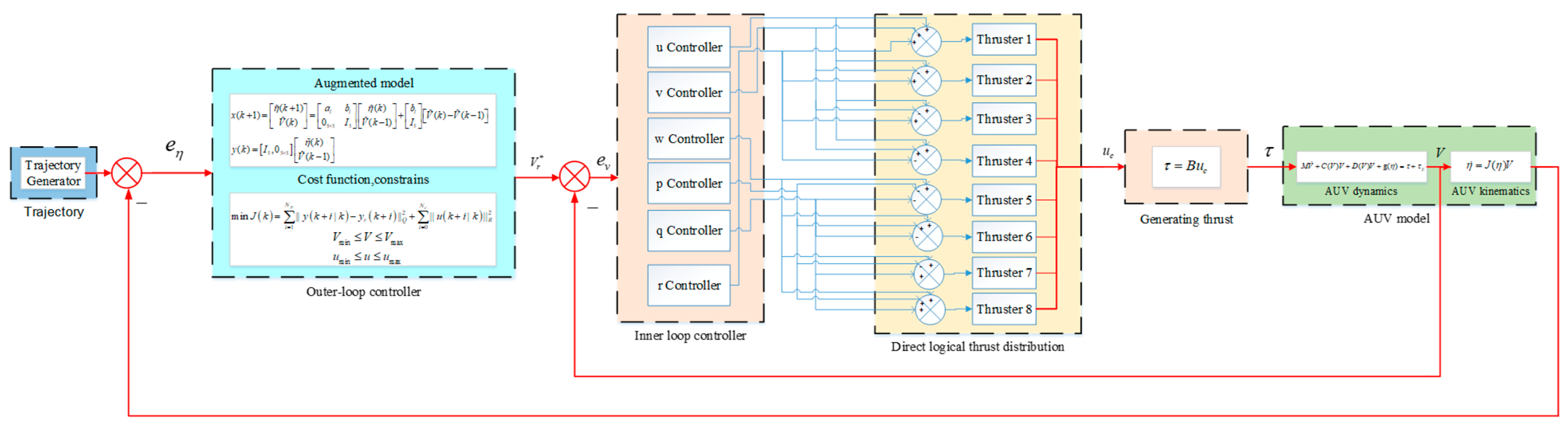
Establishing a 3-D path tracking control model is the basis for designing kinematic and dynamic controllers. This paper, on the basis of the kinematic position error tracking control model, considers the constraints of the actual speed and the speed variation of the propeller and designs an outer-loop position controller, which calculates the optimal desired speed to ensure the convergence of the AUV’s position tracking error. On the basis of the dynamic control model, a multi-channel speed controller is designed to form an inner-loop speed controller. The inner-loop speed controller outputs the desired rotational speed command and then uses the Direct Thrust Allocation method to drive the AUV, enabling the AUV’s actual speed to rapidly and stably converge to the desired speed. Under the control of the dual-loop controller, the over-actuated AUV can ultimately achieve 3-D trajectory tracking under uncertain ocean current disturbances.

The control design framework of the entire dual-loop system is shown in Figure 3. Wherein $V_r^{\ast }$ represents the desired velocity value for the inner-loop.

3.1. Design of the Kinematic Controller

The reference trajectory in this paper is a time-varying trajectory, where it is assumed that the upper-layer reference trajectory and reference control input are given by the real-time solution of the upper-layer path planning algorithm, that is, at any time $t$. there is

$${\eta }_d(t)={\left[x_d(t),y_d(t),z_d(t),{\theta }_d(t),{\psi }_d(t)\right]}^T$$

(33)

$$V_d(t)={\left[u_d(t),v_d(t),w_d(t),q_d(t),r_d(t)\right]}^T$$

(34)

$${\dot{\eta }}_d(t)=J({\eta }_d)V_d(t)$$

(35)

Based on Equation (25), we linearize the nonlinear kinematic equation shown in Equation (24) at the reference trajectory point $({\eta }_d,V_d)$, thus obtaining the following expression:

$$\begin{array}{l}\dot{\tilde{\eta }}=\left[\begin{array}{c}\dot{x}(t)-{\dot{x}}_d(t)\\ \dot{y}(t)-{\dot{y}}_d(t)\\ \dot{z}(t)-{\dot{z}}_d(t)\\ \dot{\theta }(t)-{\dot{\theta }}_d(t)\\ \dot{\psi }(t)-{\dot{\psi }}_d(t)\end{array}\right]=a\tilde{\eta }+\mathrm{b}\tilde{v}=\left[\begin{array}{ccccc}0& 0& 0& a_{14}& a_{15}\\ 0& 0& 0& a_{24}& a_{25}\\ 0& 0& 0& a_{34}& 0\\ 0& 0& 0& 0& 0\\ 0& 0& 0& 0& 0\end{array}\right]\left[\begin{array}{c}x(t)-x_d(t)\\ y(t)-y_d(t)\\ z(t)-z_d(t)\\ \theta (t)-{\theta }_d(t)\\ \psi (t)-{\psi }_d(t)\end{array}\right]\\ +\left[\begin{array}{ccccc}{b}_{11}& b_{12}& b_{13}& 0& 0\\ b_{21}& b_{22}& b_{23}& 0& 0\\ b_{31}& 0& b_{33}& 0& 0\\ 0& 0& 0& 1& 0\\ 0& 0& 0& 0& b_{55}\end{array}\right]\left[\begin{array}{c}u(t)-u_d(t)\\ v(t)-v_d(t)\\ w(t)-w_d(t)\\ q(t)-q_d(t)\\ r(t)-r_d(t)\end{array}\right]\end{array}$$

(36)

where $a_{14}=-u_d\sin {\theta }_d\cos {\psi }_d+w_d\cos {\theta }_d\cos {\psi }_d$, $a_{24}=-u_d\sin {\theta }_d\sin {\psi }_d+w_d\cos {\theta }_d\sin {\psi }_d$,

$a_{34}=-u_d\cos {\theta }_d-w_d\sin {\theta }_d$, $a_{15}=-u_d\cos {\theta }_d\sin {\psi }_d-v_d\cos {\psi }_d-w_d\sin {\theta }_d\sin {\psi }_d$,

$a_{25}=u_d\cos {\theta }_d\cos {\psi }_d-v_d\sin {\psi }_d+w_d\sin {\theta }_d\cos {\psi }_d$, $b_{11}=\cos {\theta }_d\cos {\psi }_d$, $b_{12}=-\sin {\psi }_d$,

$b_{13}=\sin {\theta }_d\cos {\psi }_d$, $b_{21}=\cos {\theta }_d\sin {\psi }_d$, $b_{22}=\cos {\psi }_d$, $b_{23}=\sin {\theta }_d\sin {\psi }_d$, $b_{31}=-\sin {\theta }_d$,

$b_{33}=\cos {\theta }_d$, $b_{55}=\frac{1}{\cos {\theta }_d}$.

In order to design the predictive controller, we use the Euler forward equation to discretize Equation (36):

$$\tilde{\eta }(k+1)=a_l\tilde{\eta }(k)+b_l\tilde{V}(k)$$

(37)

where $a_l=I_5+aT$, $b_l=bT$, $I_5$ represents the identity matrix of order 5 and $T$ denotes the sampling time.

The error in actual modeling and the process noise present when the AUV is working underwater are considered in order to enhance robustness and eliminate static error in the steady state. In predictive control based on state–space equations, a state–space model based on augmented state is adopted, introducing the increment of control input $\mathrm{u}(k)=\tilde{V}(k)-\tilde{V}(k-1)$ and resetting the state variable of the controlled system as $x(k)={\left[\tilde{\eta }(k),\tilde{V}(k-1)\right]}^T$, with Equation (37) thus becoming

$$x(k+1)=\left[\begin{array}{c}\tilde{\eta }(k+1)\\ \tilde{V}(k)\end{array}\right]=\left[\begin{array}{cc}{a}_l& b_l\\ 0_{5\times 5}& I_5\end{array}\right]\left[\begin{array}{c}\tilde{\eta }(k)\\ \tilde{V}(k-1)\end{array}\right]+\left[\begin{array}{c}{b}_l\\ I_5\end{array}\right]\left[\tilde{V}(k)-\tilde{V}(k-1)\right]=Ax(k)+Bu(k)$$

(38)

where $A=\left[\begin{array}{cc}{a}_l& b_l\\ 0_{5\times 5}& I_5\end{array}\right],$$B=\left[\begin{array}{c}{b}_l\\ I_5\end{array}\right]$

Let

$$y(k)=Cx(k)$$

(39)

In Equation (39), $C=\left[I_5,0_{5\times 5}\right]$.

Combining Equations (38) and (39), the augmented state–space representation of the controlled system is provided by

$$\{\begin{array}{c}x(k+1)=Ax(k)+Bu(k)\\ y(k)=Cx(k)\end{array}$$

(40)

(1)

Future State Prediction of the System

Assume the prediction horizon to be $N_p$ and the control horizon to be $N_c(N_p\ge N_c)$. By multi-step derivation of Equation (38), the state prediction value within the $N_p$ time domain of the system is

$$\begin{array}{l}x(k+1)=Ax(k)+Bu(k)\\ x(k+2)=Ax(k+1)+Bu(k+1)=A^{2}x(k)+ABu(k)+Bu(k+1)\\ x(k+3)=Ax(k+2)+Bu(k+2)=A^{3}x(k)+A^{2}Bu(k)+ABu(k+1)+Bu(k+2)\\ ⋮\\ x(k+Nc)=Ax(k+Nc)+Bu(k+Nc)=A^{Nc}x(k)+A^{Nc-1}Bu(k)+A^{Nc-2}Bu(k+1)+\cdots +A^{0}Bu(k+Nc-1)\\ ⋮\\ x(k+Np)=A^{Np}x(k)+A^{Np-1}Bu(k)+A^{Np-2}Bu(k+1)+\cdots +A^{0}Bu(k+Np-1)\end{array}$$

(41)

Similarly, by multi-step derivation of Equation (39), we obtain the output equation set within the $N_p$ time domain of the system:

$$\begin{array}{l}\mathrm{y}(k+1)=Cx(k+1)=CAx(k)+CBu(k)\\ \mathrm{y}(k+2)=CAx(k+1)+CBu(k+1)=C{A}^{2}x(k)+CABu(k)+CBu(k+1)\\ \mathrm{y}(k+3)=CAx(k+2)+CBu(k+2)=C{A}^{3}x(k)+C{A}^{2}Bu(k)+CABu(k+1)+CBu(k+2)\\ ⋮\\ y(k+Nc)=CAx(k+Nc)+CBu(k+Nc)=C{A}^{Nc}x(k)+C{A}^{Nc-1}Bu(k)+C{A}^{Nc-2}Bu(k+1)+\cdots +C{A}^{0}Bu(k+Nc-1)\\ ⋮\\ y(k+Np)=C{A}^{Np}x(k)+C{A}^{Np-1}Bu(k)+C{A}^{Np-2}Bu(k+1)+\cdots +C{A}^{0}Bu(k+Np-1)\end{array}$$

(42)

For the output equation set in Equation (42), let

$$Y=\left[\begin{array}{c}\mathrm{y}(k+1)\\ \mathrm{y}(k+2)\\ \cdots \\ y(k+Nc)\\ \cdots \\ y(k+Np)\end{array}\right]$$

(43)

$$\mathrm{\Psi }=\left[\begin{array}{c}CA\\ C{A}^2\\ \cdots \\ C{A}^{N\mathrm{c}}\\ \cdots \\ C{A}^{N\mathrm{p}}\end{array}\right]$$

(44)

$$U=\left[\begin{array}{c}\mathrm{u}(k)\\ \mathrm{u}(k+1)\\ \mathrm{u}(k+1)\\ \cdots \\ \mathrm{u}(k+Nc-1)\end{array}\right]$$

(45)

$$\mathrm{\Theta }=\left[\begin{array}{ccccc}CB& 0& 0& \cdots & 0\\ CAB& CB& 0& \cdots & 0\\ \cdots & \cdots & \cdots & \ddots & \cdots \\ C{A}^{N\mathrm{c}}-{}^{1}B& C{A}^{N\mathrm{c}}-{}^{2}B& C{A}^{N\mathrm{c}}-{}^{3}B& \cdots & C{A}^{0}B\\ \cdots & \cdots & \cdots & \ddots & \cdots \\ C{A}^{Np}-{}^{1}B& C{A}^{Np}-{}^{2}B& C{A}^{Np}-{}^{3}B& \cdots & C{A}^{Np-Nc}B\end{array}\right]$$

(46)

Thus, the output equation can be written in a more compact form:

$$Y=\mathrm{\Psi }x(k)+\mathrm{\Theta }U$$

(47)

Therefore, if the state quantity at the current moment is known, as well as the control increment within the $N_c$ control horizon, it is also possible to predict the system output within the future $N_p$ time domain.

(2)

Constrained Optimization for an AUV System’s Predictive Controller

As it is an error equation that has been established, the control target is to gradually converge the tracking error of the reference trajectory. Therefore, the reference value of the system output can be defined as

$$Y_r={\left[\begin{array}{cccccc}{\mathrm{y}}_r(k+1)& {\mathrm{y}}_r(k+2)& \cdots & y_r(k+Nc)& \cdots & y_r(k+Np)\end{array}\right]}^T={\left[\begin{array}{cccccc}0& 0& \cdots & 0& \cdots & 0\end{array}\right]}^T$$

(48)

The optimization objective function can be defined as

$$\min J\left(k\right)={\displaystyle \sum _{i=1}^{N_p}\left|\right|y\left(k+i|k\right)-y_r\left(k+i\right)|{|}_Q^2}+{\displaystyle \sum _{i=0}^{N_c}\left|\right|u\left(k+i|k\right)|{|}_R^2}$$

(49)

where $Q$ and $R$ respectively represent the weighting matrices of the output signal and the control signal.

Let $E=\mathrm{\Psi }x(k)$, $Q_Q=I_{N_{\mathrm{p}}}\otimes Q$, $R_R=I_{N_{\mathrm{p}}}\otimes R$, and $\tilde{Y}=\left(Y-Y_r\right)$, where the symbol $\otimes$ represents the Kronecker product.

Thus,

$$\begin{array}{l}\min J\left(k\right)={\tilde{Y}}^T{Q}_Q\tilde{Y}+U^T{R}_{R}U\\ ={(Y-Y_{\mathrm{r}})}^T{Q}_Q(Y-Y_{\mathrm{r}})+U^T{R}_{R}U\\ ={[\mathrm{\Psi }x(k)+\mathrm{\Theta }U-Y_{\mathrm{r}}]}^T{Q}_Q[\mathrm{\Psi }x(k)+\mathrm{\Theta }U-Y_{\mathrm{r}}]+U^T{R}_{R}U\\ =U^T({\mathrm{\Theta }}^T{Q}_Q\mathrm{\Theta }+R_R)U+2E^T{Q}_Q\mathrm{\Theta }U+E^T{Q}_{Q}E-Y_{\mathrm{r}}{Q}_Q\mathrm{\Theta }U+{Y^T}_{\mathrm{r}}{Q}_{Q}Y-2{Y^T}_{\mathrm{r}}{Q}_{Q}E\end{array}$$

(50)

Since $E^T{Q}_{Q}E-Y_{\mathrm{r}}{Q}_Q\mathrm{\Theta }U+{Y^T}_{\mathrm{r}}{Q}_{Q}Y-2{Y^T}_{\mathrm{r}}{Q}_{Q}E$ is a constant, it can be omitted when solving the objective function.

If we let $H={\mathrm{\Theta }}^T{Q}_Q\mathrm{\Theta }+R_R$ and $\mathrm{g}=E^T{Q}_Q\mathrm{\Theta }$, then the objective function can be rewritten as

$$\underset{U}{\min } J=2(\frac{1}{2}{U}^{T}HU+{\mathrm{g}}^{T}U)\iff \underset{U}{\min } J=\frac{1}{2}{U}^{T}HU+{\mathrm{g}}^{T}U$$

(51)

For the control quantity and control increment, the following recursive formulas exist:

$$\begin{array}{l}\tilde{V}(k)=\tilde{V}(k-1)+\mathrm{u}(k)\\ \tilde{V}(k+1)=\tilde{V}(k)+\mathrm{u}(k+1)=\tilde{V}(k-1)+\mathrm{u}(k)+\mathrm{u}(k+1)\\ \cdots \\ \tilde{V}(k+Nc-1)=\tilde{V}(k+Nc-2)+\mathrm{u}(k+Nc-1)=\tilde{V}(k-1)+\mathrm{u}(k)+\mathrm{u}(k+1)+\cdots \mathrm{u}(k+Nc-1)\end{array}$$

(52)

The above equation can be rewritten as

$$V_A=\left[\begin{array}{c}\tilde{V}(k)\\ \tilde{V}(k+1)\\ \tilde{V}(k+1)\\ \cdots \\ \tilde{V}(k+Nc-1)\end{array}\right]=\left[\begin{array}{c}\tilde{V}(k-1)\\ \tilde{V}(k-1)\\ \tilde{V}(k-1)\\ \cdots \\ \tilde{V}(k-1)\end{array}\right]+\left[\begin{array}{ccccc}{I}_2& 0& 0& \cdots & 0\\ I_2& I_2& 0& \cdots & 0\\ I_2& I_2& I_2& \cdots & 0\\ \cdots & \cdots & \cdots & \ddots & 0\\ I_2& I_2& I_2& \cdots & I_2\end{array}\right]\left[\begin{array}{c}\mathrm{u}(k)\\ \mathrm{u}(k+1)\\ \mathrm{u}(k+2)\\ \cdots \\ \mathrm{u}(k+N\mathrm{c}-1)\end{array}\right]=V_T+A_{I}U$$

(53)

Due to the power limitation of the thruster and the influence of the underwater drag environment, the velocity and velocity increment of the AUV are bounded. Let the amplitude of the control input in the state variable have an upper bound $V_{\max }$ and a lower bound $V_{\min }$, and let the amplitude of the control input increment $u(k)$ have an upper bound $u_{\max }$ and a lower bound $u_{\min }$.

$$u_{\min }\le u(k)\le u_{\max }$$

(54)

$$V_{\min }\le V_A\le V_{\max }$$

(55)

The amplitude of the control input increment U is also finite, respectively set as the upper bound $U_{\max }$ and the lower bound $U_{\min }$. Hence, the following inequality constraints of control input can be obtained:

$$V_{\min }\le V_T+A_{I}U\le V_{\max }\to \{\begin{array}{c}{A}_{I}U\le V_{\max }-V_T\\ -A_{I}U\le -V_{\min }+V_T\end{array}$$

(56)

$$U_{\min }\le U\le U_{\max }$$

(57)

In summary, the problem of predictive 3-D trajectory tracking control for the AUV has been transformed into a standard quadratic programming (QP) problem:

$$\begin{array}{l}{U}^{\ast }\left(k\right)=\underset{U}{\min } J=\frac{1}{2}{U}^{T}HU+{\mathrm{g}}^{T}U\\ \mathrm{s}.t.\{\begin{array}{c}{A}_{I}U\le V_{\max }-V_T\\ -A_{I}U\le -V_{\min }+V_T\\ U_{\min }\le U\le U_{\max }\end{array}\end{array}$$

(58)

By solving the QP problem, the optimal control action $U^{\ast }\left(k\right)$ within the $Nc$ domain at each moment can be obtained. The first element $u^{\ast }(k)$ in the vector $U^{\ast }\left(k\right)$ is taken as the optimal control action at moment $k$. Since $u^{\ast }(k)$ is the optimal control increment input, it needs to go through the following formula to obtain the optimal reference value $V_r^{\ast }(k)$ of linear velocity and angular velocity at the current sampling time $k$.

$$V_r^{\ast }(k)=\tilde{V}(k-1)+u^{\ast }(k)+V_d\left(k\right)$$

(59)

$$V_r^{\ast }(k)={\left[\begin{array}{c}{u}_r\\ v_r\\ w_r\\ q_r\\ r_r\end{array}\right]}_k$$

(60)

Up to this point, the design of the outer-loop kinematic controller has been completed. Take $V_r^{\ast }(k)$ as the reference value for the dynamic controller. Next, the design of the inner-loop dynamic controller will commence.

3.2. Design of the Dynamic Controller

Before the advent of variable universe fuzzy control algorithms, fuzzy control algorithms were considered a crude control method, as the division of fuzzy sets cannot be infinitely numerous and fuzzy rules are generally fixed. Hongxing Li proposed the variable universe fuzzy controller and successfully applied this method to control a nonlinear system, specifically a quadruple inverted pendulum [38]. The variable universe fuzzy controller introduces the concept of variable universes based on traditional fuzzy control theory [39]. By designing suitable scaling factors to control the expansion and contraction of the universe of discourse, the controller can still perform with high precision within a sufficiently small region. Meanwhile, the design of scaling discourse makes the fuzzy controller have good robustness and adaptability, which simplifies the design of the fuzzy controller [40,41]. The approximate expression for the variable universe fuzzy controller can be described as

$$\mathrm{y}=f(x/s(x))$$

(61)

where $s(x)$ represents the scaling factor, $x$ represents the input of the controller, and $\mathrm{y}$ represents the output of the controller.

This paper directly adopts well-established scaling factors, and there are primarily two commonly used forms of scaling factors.

$$s(x)={(\frac{\left|x\right|}{E})}^{\tau }+\epsilon ,\tau >0,\epsilon \mathrm{is} \mathrm{a} \mathrm{sufficiently} \mathrm{small} \mathrm{positive} \mathrm{number}.$$

(62)

$$s(x)=1-\lambda \exp (-k{x}^2),\lambda \in (0,1),k>0$$

(63)

The S-plane control strategy is based on fuzzy control ideas, replacing traditional fuzzy controllers with ‘S’-shaped function surfaces. It uses the sigmoid function to construct the S-plane controller functions, which makes the controller easier to design [29]. The classic S-plane control with nonlinear control surfaces is more suitable for the motion control of autonomous underwater vehicles.

The variable universe fuzzy controller is divided into two parts: the scaling factor part and the fuzzy logic part. For the fuzzy logic part, since the S-plane control strategy is designed based on fuzzy control theory, we attempted to combine the two, using the S-plane (which can be referred to as a basis function) as a substitute while retaining the proportional factor part, thus simplifying the variable universe fuzzy controller. This forms a new algorithm, namely the S-VUD FLC algorithm. It is a combination of variable universe fuzzy controllers and S-plane algorithms and combines the strong robustness of variable universe fuzzy controllers with the ease of constructing S-plane algorithms.

The following are the construction steps for the new algorithm:

Step1.

Use the following sigmoid function:

$$tansig(x)=\frac{e^x-e^{-x}}{e^x+e^{-x}},e \mathrm{is} \mathrm{a} \mathrm{natural} \mathrm{number}$$

(64)

Step2.

Construct the S-plane: let $x_1$ and $x_2$ be the inputs and $y$ be the output, thus leading to

$$y={\beta }_{1}tansig\left({\alpha }_1{x}_1\right)+{\beta }_{2}tansig\left({\alpha }_2{x}_2\right)$$

(65)

Step3.

The S-plane controller is represented by $y_s=f_s(X)$, where $X$ represents the input vector. The S-VUD FLC controller can be expressed as

$${y_s}^{\prime }=f_{\mathrm{s}}(\frac{x_1}{\alpha (x_1)},\frac{x_2}{\alpha (x_2)})/\beta (pX),p=[0.5,0.5]$$

(66)

$$\alpha (x)=1-\gamma \exp \left(-0.5x^2\right)(\gamma <1),\beta (pX) \mathrm{ensures} \mathrm{that} {y_s}^{\prime } \mathrm{is} \mathrm{sufficiently} \mathrm{large}$$

(67)

$$f_s(X)=\lambda tansig \left(c{x}_1\right)+(1-\lambda )tansig\left(c{x}_2\right)$$

(68)

In the above formula, $\alpha (x)$ and $\beta (pX)$ represent the scaling factors for the input and output ends, respectively (which can degenerate into gain if fixed values are taken), and $p$ is the weight vector. Thus, the S-VUD FLC algorithm can be represented as a combination of an S-plane function and scaling factors. The factor $c$ can cause horizontal axis scaling, changing the effective range of the input. The factor $\lambda$ can change the weight of the input; when input noise is significant, it is necessary to increase the weight of the error to reduce the noise impact.

The action of the scaling factors also affects control performance. The closer $\gamma$ is to 1, the steeper the controller’s change, the smaller the steady-state error, and the quicker the response, but with stronger oscillations; the smaller $\gamma$ is, the gentler the controller’s change, the slower the response speed, and the smaller the oscillations. Therefore, the tightness of the scaling factor is an important parameter affecting controller performance. According to simulation test results, the scaling factor $\gamma$ in the above formula should preferably be chosen between 0.8 and 0.9.

To reduce the steady-state error of the system, enhance the ability to resist disturbances in the uncertain underwater environment, and improve the stability of the system, we draw on the design concept of PID controllers to improve S-VUD FLC. By introducing an integral term into the expression of S-VUD FLC, we name the new controller as the Improved Variable Universe S-plane Controller (P-S-VUD FLC). The expression is as follows:

$${y_s}^{\prime }=f_{\mathrm{s}}(\frac{x_1}{\alpha (x_1)},\frac{x_2}{\alpha (x_2)})/\beta (pX)+K_i{\displaystyle \underset{0}{\overset{\mathrm{t}}{\int }}{x}_{2}dt},p=[0.5,0.5]$$

(69)

$$\alpha (x)=1-\gamma \exp \left(-0.5x^2\right)(\gamma <1),\beta (pX) \mathrm{ensures} \mathrm{that} {y_s}^{\prime }\mathrm{is} \mathrm{sufficiently} \mathrm{large}$$

(70)

$$f_s(X)=\lambda tansig \left(c{x}_1\right)+(1-\lambda )tansig\left(c{x}_2\right)$$

(71)

In Equation (69), $K_i$ is the coefficient of the integral term.

The new controller combines the strong robustness of variable universe fuzzy controllers and the easy-to-construct characteristics of S-plane algorithms. The advantages are quite obvious: it greatly simplifies the design of variable universe fuzzy controllers, making the controller’s design more flexible and easier to implement. It is very convenient for model simulation, and performance analysis and optimization of the system are more straightforward, accelerating the development and validation process of the control algorithm.

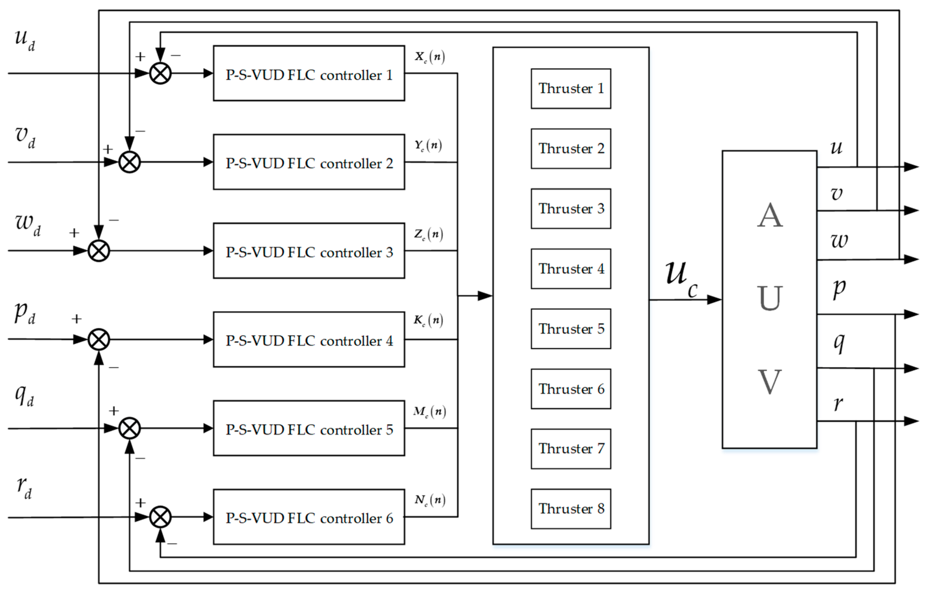
Below is the design process of the P-S-VUD FLC for the over-actuated AUV:

Step1.

Let the difference between the desired velocity ${\mathrm{V}}_{\mathrm{r}}^{\ast }(\mathrm{k})$ generated by the outer-loop kinematic controller and the actual velocity $V(k)$ sensed by the sensors be denoted as $e_V$. The derivative of $e_V$ is denoted as ${\dot{e}}_V$.

Thus,

$$e_V=V_r^{\ast }(k)-V(k)={\left[\begin{array}{c}{u}_r-u\\ v_r-v\\ w_r-w\\ q_r-q\\ r_r-r\end{array}\right]}_k$$

(72)

Step2.

The velocity deviation $e_V$ and its derivative ${\dot{e}}_V$ are used as inputs to the inner-loop dynamic controller. If we let $p_r=0$, then $e_V$ can be rewritten as follows:

$$e_V={\left[\begin{array}{c}{u}_r-u\\ v_r-v\\ w_r-w\\ p_r-p\\ q_r-q\\ r_r-r\end{array}\right]}_k$$

(73)

Step3.

P-S-VUD FLC is designed for each degree of freedom of the AUV, and these six improved Variable Universe S-plane controllers together form the inner-loop dynamic controller, as shown in Figure 4.

We will verify the stability and effectiveness of the designed dynamic control through simulation experiments in Section 4.

3.3. Stability Proof of the Kinematic Controller

In this section, the stability proof of the outer-loop controller is presented.

Theorem 1.

Consider the optimization objective function (51) under constraint condition (56), choose the positive-definite matrix for weighting factors $Q$ and $R$, prediction horizon $N_p$ and control horizon $N_c$, to ensure the existence of the optimal solution for the optimization objective function (51). Choose the optimal cost function $J^{\ast }\left(k\right)$ as the Lyapunov function $V^{\ast }\left(k\right)$. If the condition $V^{\ast }\left(k+1\right)\le V^{\ast }\left(k\right)$ is satisfied, the optimal solution $U^{\ast }\left(k\right)$ ensures nominal stability of the system (37).

Proof of Theorem 1.

In the optimal solution $U^{\ast }\left(k\right)$ of the optimization objective function (51) under constraint condition (56), choose $u^{\ast }(k+i|k)$ as the optimal control input. ${\tilde{V}}^{\ast }(k+i|k)$ is then the optimal control input corresponding to the optimal control input increment $u^{\ast }(k+i|k)$. Choose the optimal objective function $J^{\ast }\left(k\right)$ as the Lyapunov function $V^{\ast }\left(k\right)$.

$$\begin{array}{l}{V}^{\ast }\left(k\right)=\min J\left(k\right)\\ =\min \left[{\displaystyle \sum _{i=1}^{N_p}\left|\right|x\left(k+i|k\right)-x_d\left(k+i\right)|{|}_Q^2}+{\displaystyle \sum _{i=0}^{N_c-1}\left|\right|u\left(k+i|k\right)|{|}_R^2}\right]\end{array}$$

(74)

Obviously, the optimal function (74) satisfies $V^{\ast }\left(0\right)=0$ and $k=0$, $V^{\ast }\left(k\right)>0$ and $k\ne 0$. For system (37) with external disturbances, the optimal control input increment $u(k+1+i|k+1)$ and control input $\tilde{V}(k+1+i|k+1)$ are as follows:

$$\begin{array}{l}u(k+1+i|k+1)=\left[u(k+1|k+1),u(k+2|k+1),\dots ,u(k+N_c|k+1)\right]\\ =\left[u^{\ast }(k+1|k+1),u^{\ast }(k+2|k+1),\dots ,u^{\ast }(k+N_c|k+1)\right]\end{array}$$

(75)

$$\begin{array}{l}\tilde{V}(k+1+i|k+1)=\left[\tilde{V}(k+1|k+1),\tilde{V}(k+2|k+1),\dots ,\tilde{V}(k+N_c|k+1)\right]\\ =\left[{\tilde{V}}^{\ast }(k+1|k+1),{\tilde{V}}^{\ast }(k+2|k+1),\dots ,{\tilde{V}}^{\ast }(k+N_c|k+1)\right]\end{array}$$

(76)

It is easy to prove that (75) and (76) are feasible solutions to the quadratic programming problem (58). The control increment $u(k+1+i|k+1)$ and control variable $\tilde{V}(k+1+i|k+1)$ satisfy constraint sets (54) and (55), respectively. Based on (75) and (76), the relationship between $V^{\ast }\left(k\right)$ and $J\left(k+1\right)$ is as follows:

$$V^{\ast }\left(k+1\right)\le J\left(k+1\right)\le V^{\ast }\left(k\right)-\left|\right|y\left(k+i|k\right)-y_r\left(k+i\right)|{|}_Q^2-|\left|u\left(k+i|k\right)\right|{|}_R^2$$

(77)

where

$$\begin{array}{l}J\left(k+1\right)={\displaystyle \sum _{i=1}^{N_p}\left|\right|y\left(k+1+i|k+1\right)-y_r\left(k+1+i\right)|{|}_Q^2}+{\displaystyle \sum _{i=0}^{N_c}\left|\right|u\left(k+1+i|k+1\right)|{|}_R^2}\\ ={\displaystyle \sum _{i=2}^{N_p}\left|\right|y^{\ast }\left(k+i|k\right)-y_r\left(k+i\right)|{|}_Q^2}+{\displaystyle \sum _{i=1}^{N_c-1}\left|\right|u^{\ast }\left(k+i|k\right)|{|}_R^2}\\ ={\displaystyle \sum _{i=1}^{N_p}\left|\right|y^{\ast }\left(k+i|k\right)-y_r\left(k+i\right)|{|}_Q^2}+{\displaystyle \sum _{i=0}^{N_c-1}\left|\right|u^{\ast }\left(k+i|k\right)|{|}_R^2}-\left|\right|y\left(k|k\right)-y_r\left(k\right)|{|}_Q^2-|\left|u\left(k|k\right)\right|{|}_R^2\\ =V^{\ast }\left(k\right)-\left|\right|y\left(k|k\right)-y_r\left(k\right)|{|}_Q^2-|\left|u\left(k|k\right)\right|{|}_R^2\end{array}$$

(78)

Additionally, due to the optional nature of the cost function (58), the function $J\left(k+1\right)$ is not less than $V^{\ast }\left(k+1\right)$.

$$V^{\ast }\left(k+1\right)\le V^{\ast }\left(k\right)$$

(79)

The Lyapunov function (74) satisfies the following requirements: when $k=0$, $V^{\ast }\left(0\right)=0$; when any $k\ne 0$, $V^{\ast }\left(k\right)>0$. Therefore, the Lyapunov function (74) is monotonically decreasing, that is, $V^{\ast }\left(k+1\right)\le V^{\ast }\left(k\right)$. In conclusion, system (37) is nominally stable, and the stability proof of the outer-loop controller based on MPC is complete. □

The stability proof of the outer-loop controller based on MPC verifies the effectiveness of the designed controller, ensuring the convergence of the system to the equilibrium point. In the next section, we will use simulation experiments to validate the proposed dual closed-loop controller, achieving three-dimensional curvilinear trajectory tracking for the “SZ-1” AUV.

4. Simulation Results and Analysis

The simulation model used in this paper is based on the “SZ-1” AUV independently developed by China University of Petroleum (Beijing). As the 3-D trajectory tracking control performance of the AUV depends on the precise establishment of the model, this paper combines hydrodynamic experiments and Ansys professional software for modeling analysis to obtain more accurate parameters for the “SZ-1” AUV model and reviews the relevant literature [42]. The obtained parameters for the “SZ-1” AUV are shown in

Table 2. Relevant parameters of the “SZ-1” AUV.

Parameter	Value
$m$	177 kg
$B$	1158 kN
$M_{RB}$	$diag\{117.0,117.0,117.0,10.7,11.8,13.4\}$
$M_{AM}$	$diag\{58.40,23.80,23.80,3.38,1.18,2.67\}$
$D(v)$	$diag\{120+90\left|u\right|,90+90\left|v\right|,150+120\left|w\right|,15+10\left|p\right|,15+12\left|q\right|,18+15\left|r\right|\}$

.

This paper used Matlab/Simulink software to build a simulation environment.

When the AUV is performing a water area survey mission in a certain water body, it is required to cruise underwater along a curved trajectory, during which it will be affected by various types of disturbances. In this paper, the simulated ocean current disturbance model ${\tau }_E$ is added to each component of the AUV linear velocity vector $V_1={\left[u,v,w\right]}^T$, as shown in Equation (80).

$${\tau }_E=\left[0.5\sin (\frac{t}{75})•\cos (\frac{t}{150})\right]$$

(80)

To validate the control performance of the designed controller for curve trajectory tracking, the curve reference trajectory is defined as Equation (81) and the initial state of the AUV is set to ${\left[0,0,0,0,0\right]}^T$.

$$Y_d(t)=\{\begin{array}{c}0.5\sin (0.8\mathrm{t})\\ 0.5-0.5\cos (0.8\mathrm{t})\\ 0.3\mathrm{t}\end{array}$$

(81)

4.1. Simulation Results without Disturbance

In order to analyze the tracking performance of the proposed control method (which uses the MPC controller as the outer loop and the P-S-VUD FLC controller as the inner loop) on the 3-D curve trajectory, the inner-loop dynamic controller is replaced with a classic PID controller while the outer-loop controller remains the same. A simulation is used to compare the tracking performance of the two methods on the reference 3-D curved trajectory.

Table 3. MPC controller design parameters.

Parameter	Value
$T\left(Sampling time\right)$	$0.0005$
$Q_i$	$100$
$R_i$	$0.1$
$N_p$	$20$
$N_c$	$10$
$V_{\max }$	$\left[0.7,0.4,0.7,1.25,1.25\right]$
$V_{\min }$	$\left[-0.7,-0.4,-0.7,-1.25,-1.25\right]$
$U_{\max }$	$\left[0.08,0.08,0.08,0.15,0.15\right]$
$U_{\min }$	$\left[-0.08,-0.08,-0.08,-0.15,-0.15\right]$

presents the design parameters of the MPC controller.

Firstly, the 3-D curve trajectory tracking simulation results of the “SZ-1” AUV under no ocean current interference are provided, as shown in the figures below. In all the following figures, Method 1 refers to the dual-loop controller based on MPC and PID, while Method 2 refers to the dual-loop controller based on MPC and the P-S-VUD FLC.

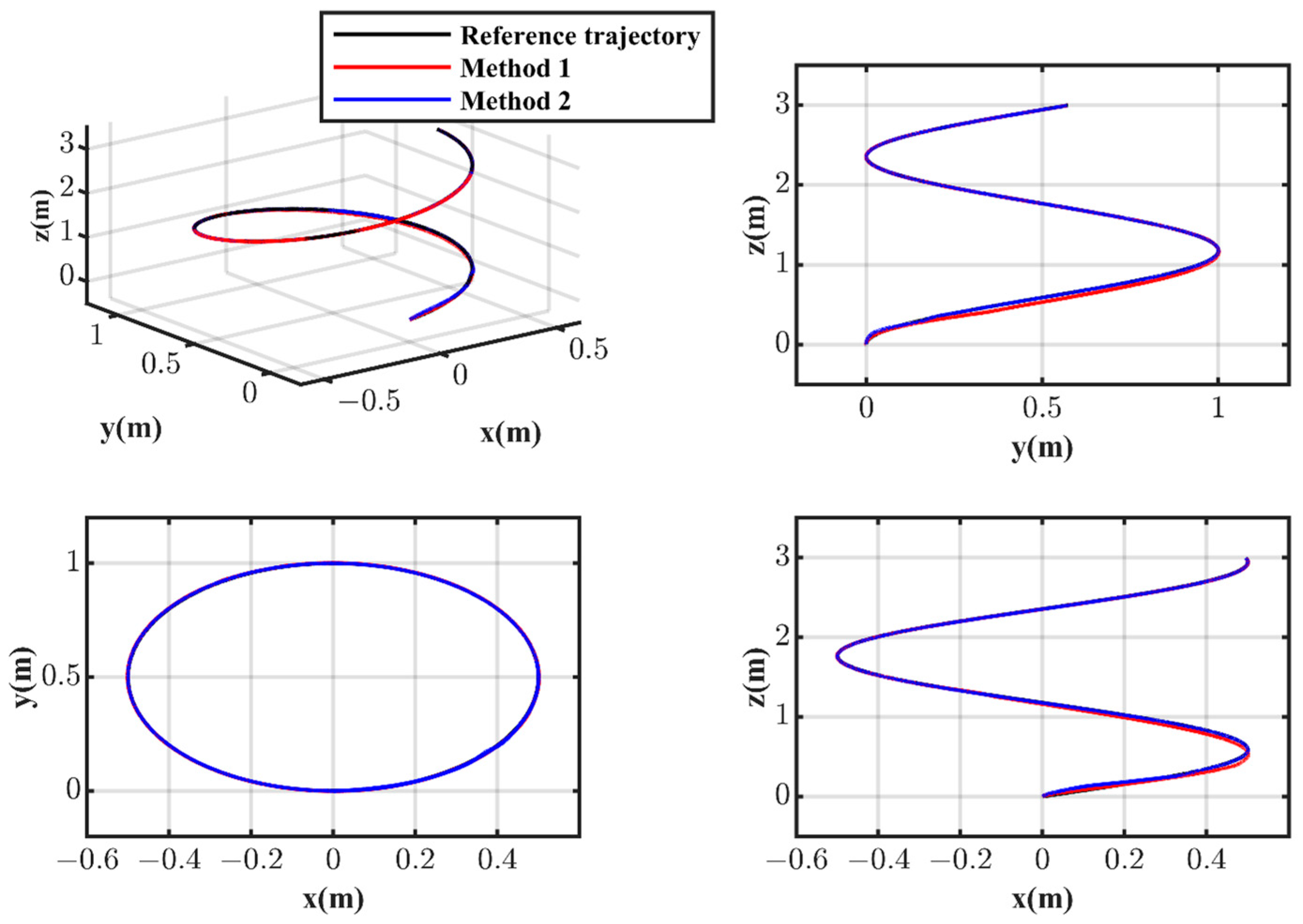
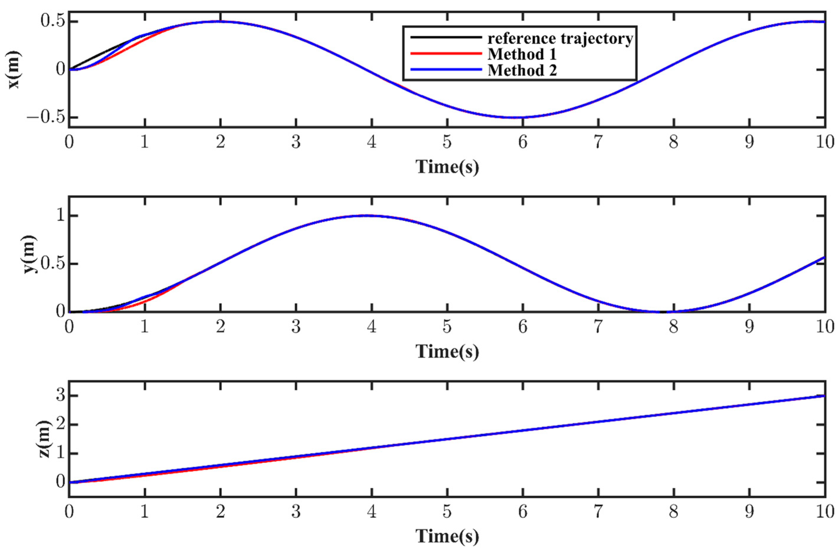
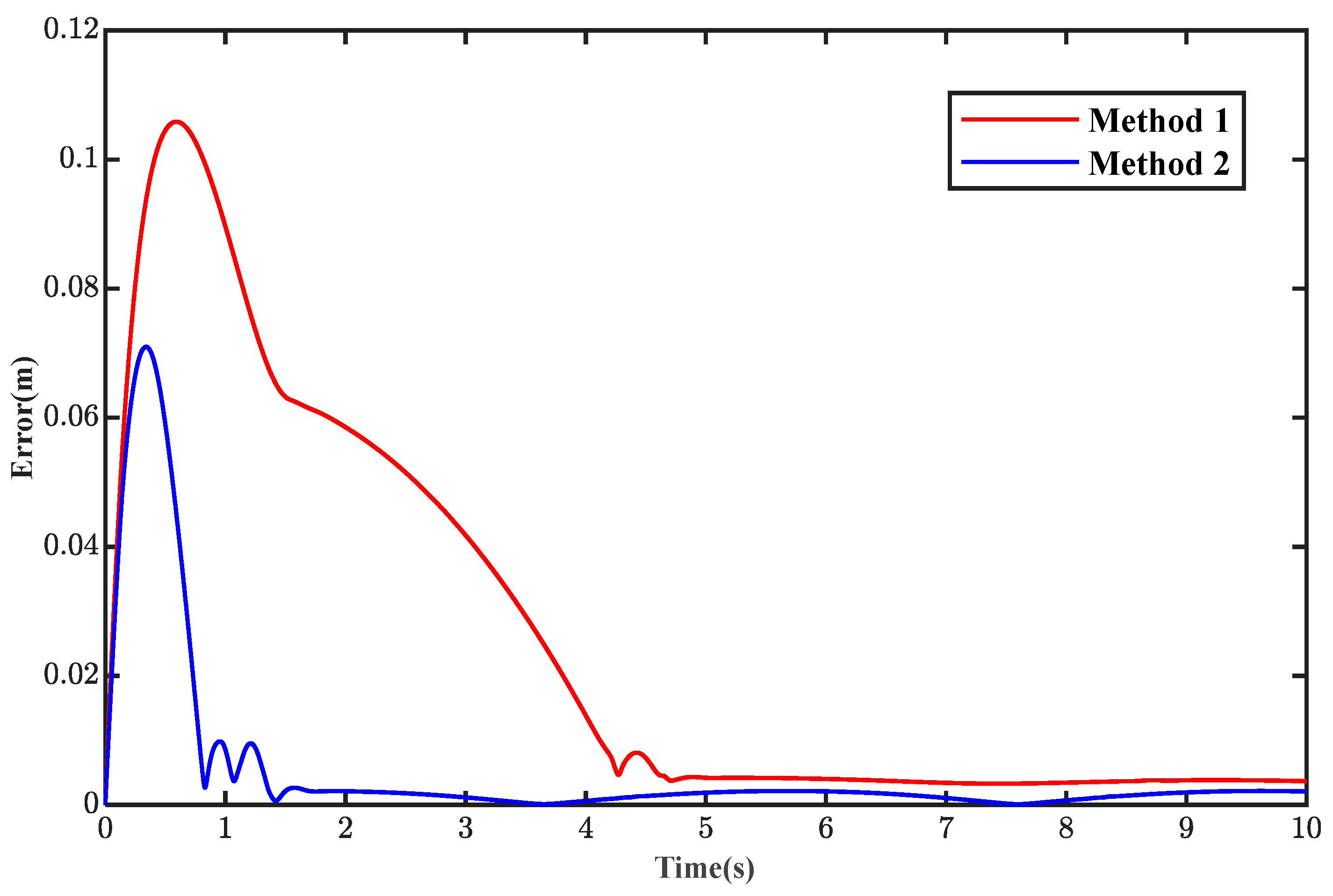
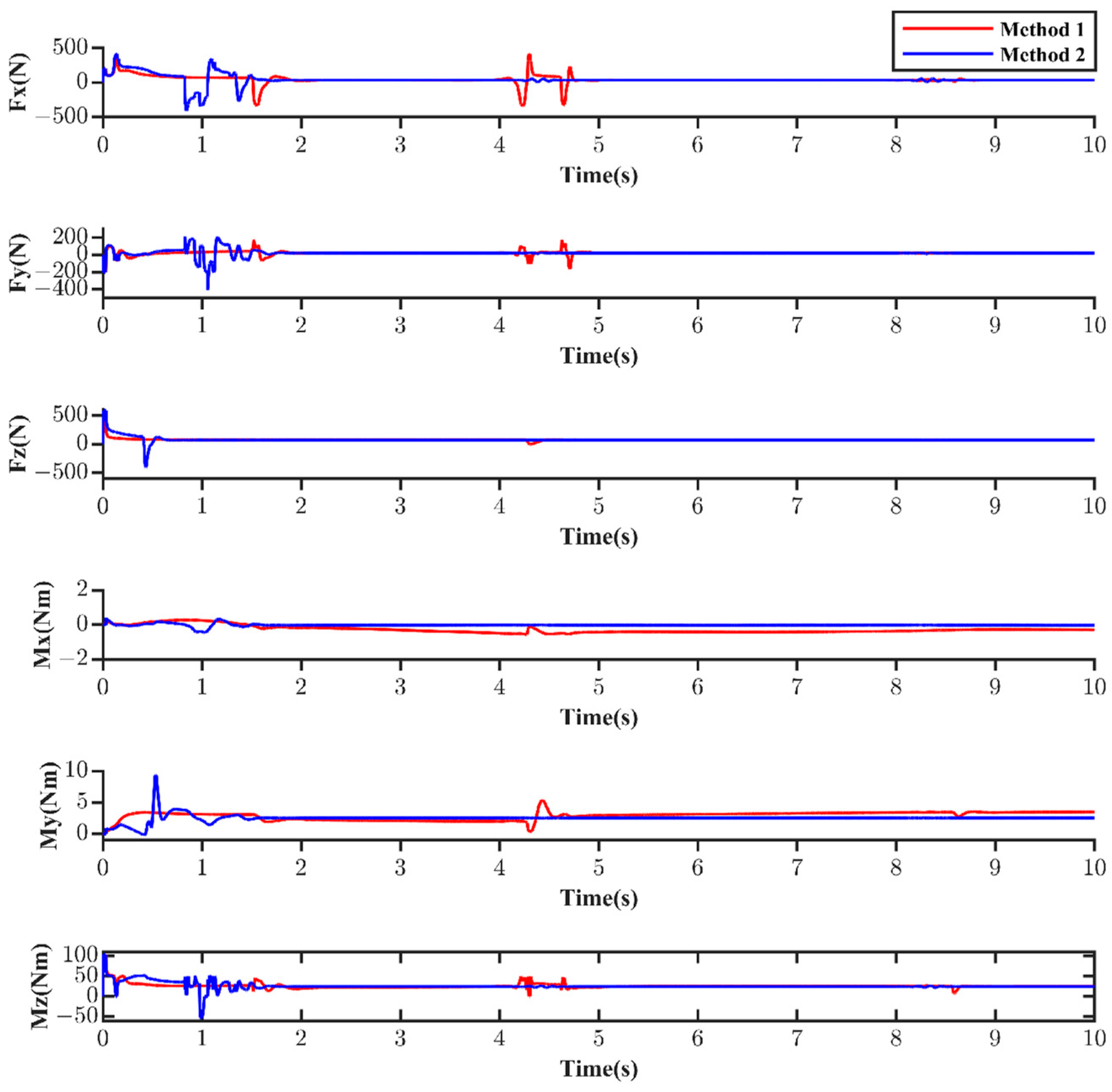
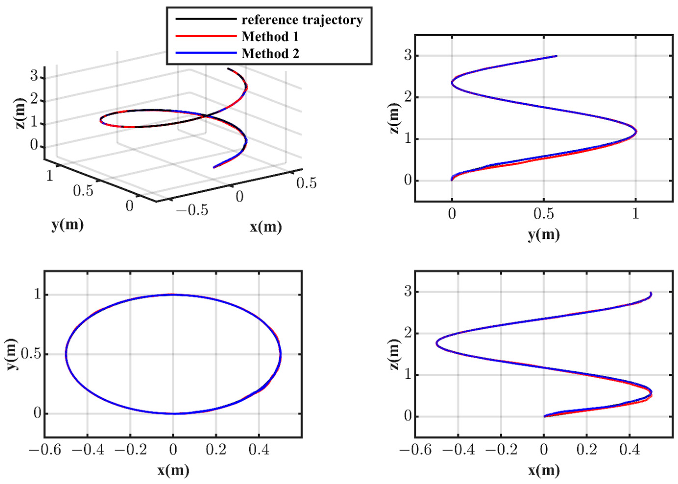
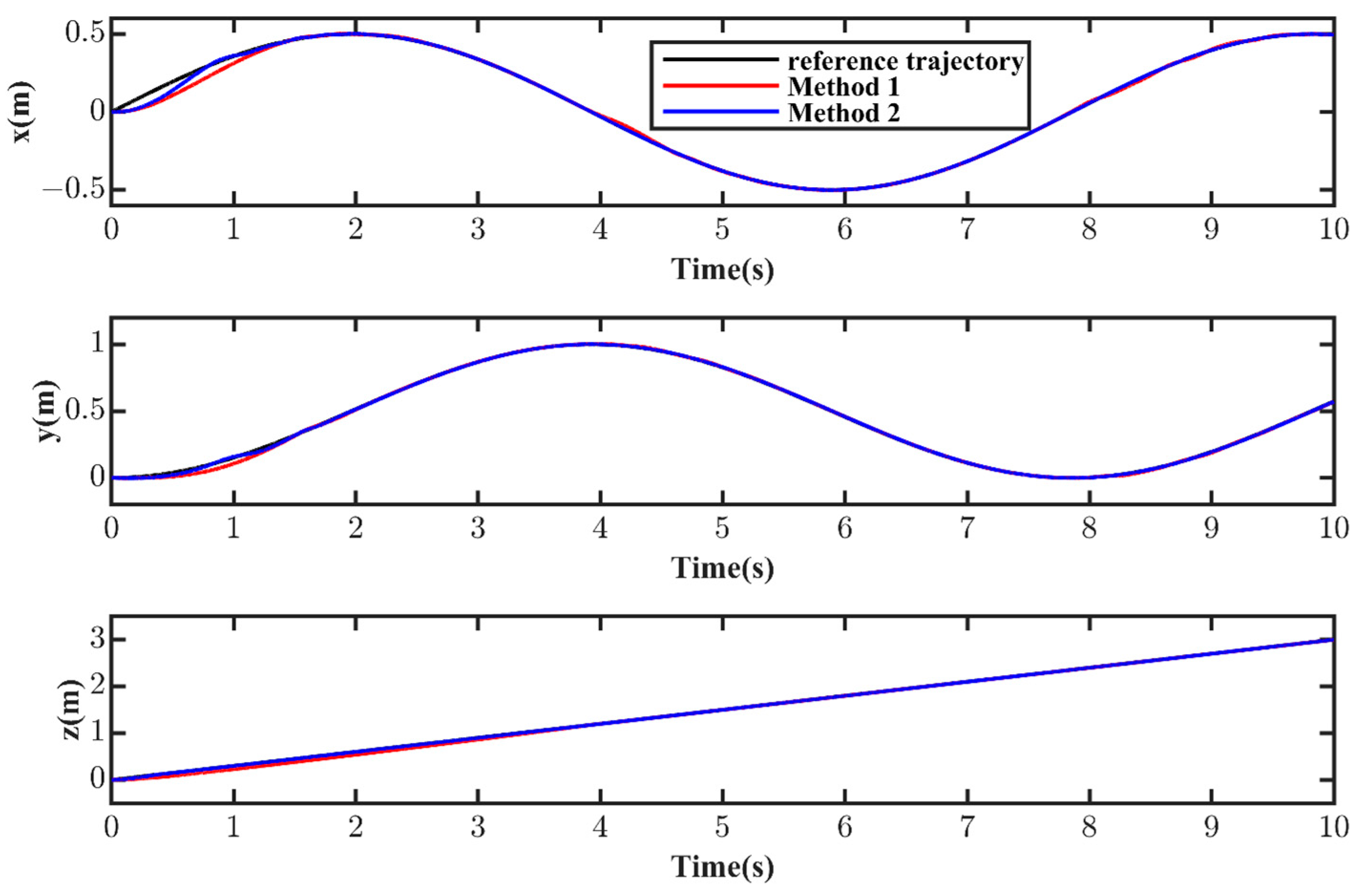
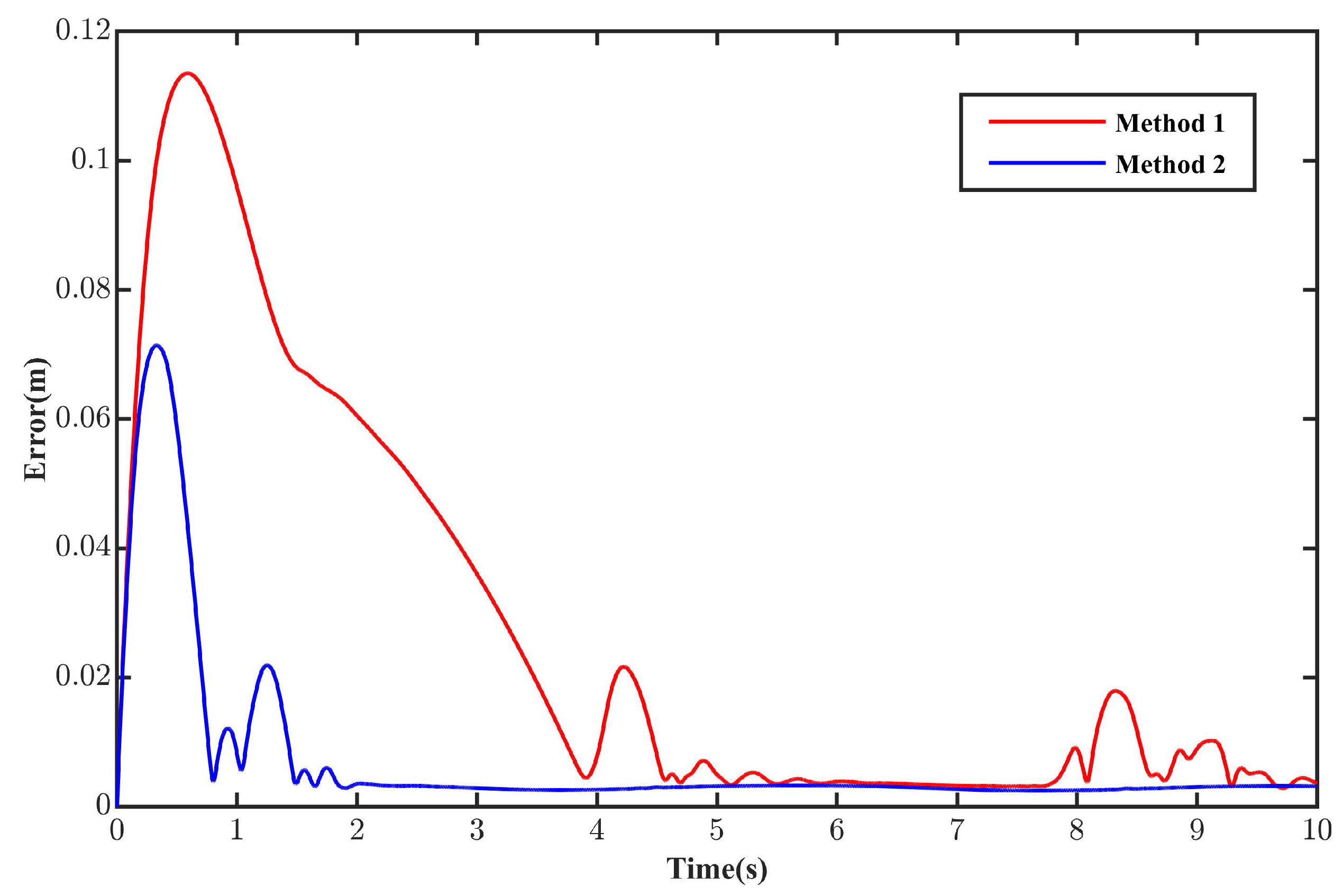
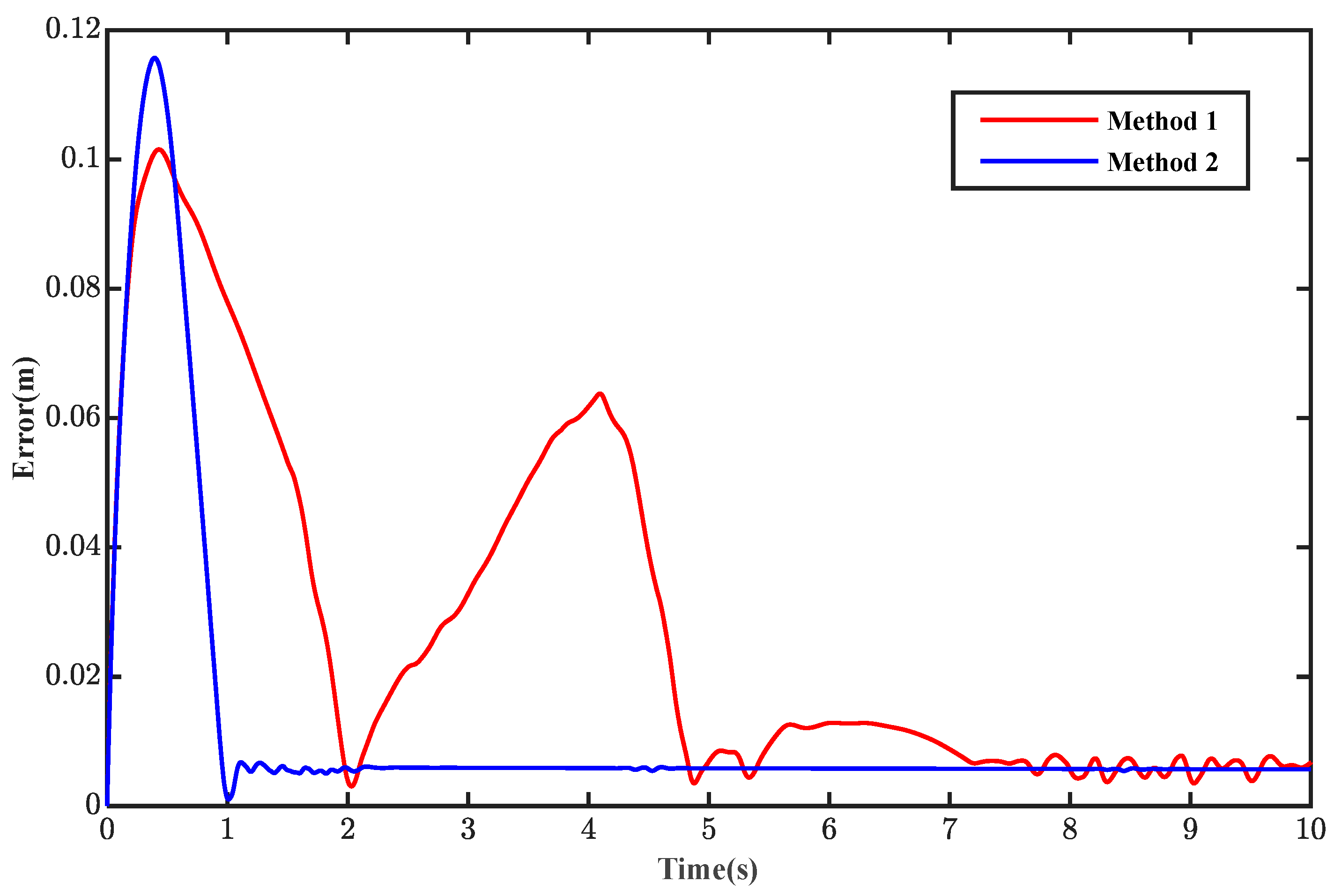
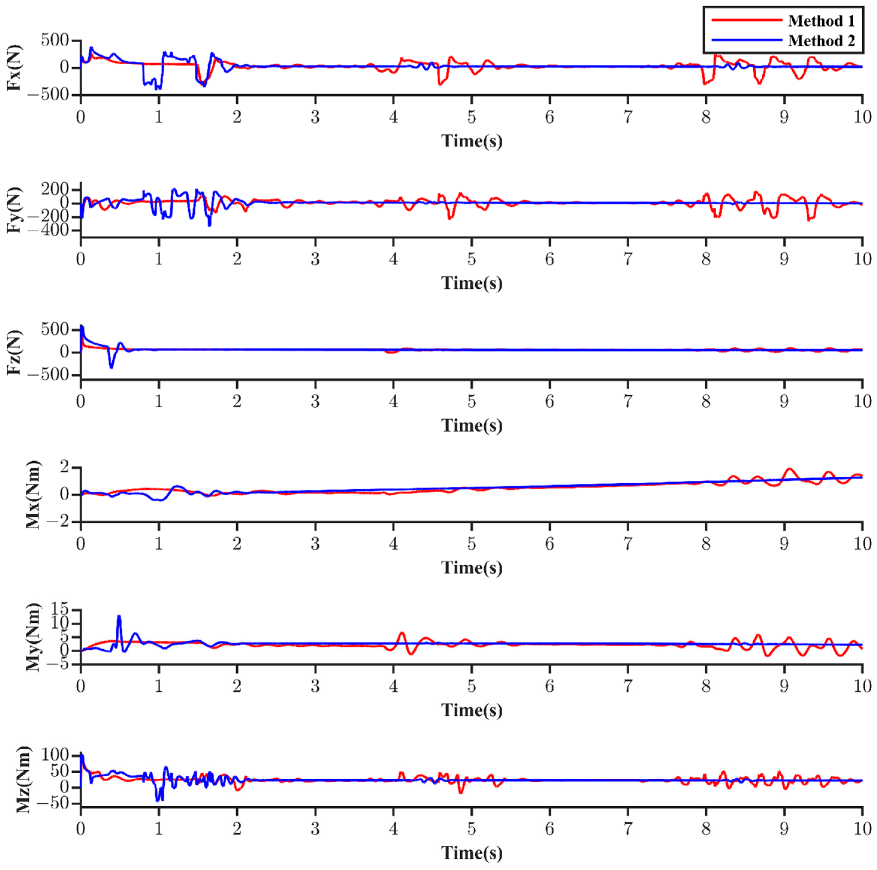
Figure 5 shows the trajectory tracking effects of the three methods on a 3-D curve in the absence of interference. The black curve is the reference trajectory, the blue curve represents the tracking effect of the conventional PID controller combined with MPC, and the red curve represents the tracking effect of the P-S-VUD FLC controller combined with MPC. To further display the details of 3-D trajectory tracking, the projection of the 3-D curve tracking effect on the two-dimensional plane is provided. Figure 6 shows the position tracking effects on the x, y, and z axes. Figure 7 and Figure 8 are the position tracking error curves and attitude tracking error curves, respectively. Combining Figure 7 and Figure 8, it can be seen that both control methods can track the 3-D curve trajectory, though by comparison Method 2 allows the AUV to track the expected 3-D curve trajectory from the initial position (0, 0, 0) faster, and the tracking error thus converges more quickly.

Table 4. Position tracking error results without disturbance.

Method	Mean Absolute Error (MAE)	Root Mean Square Error (RMSE)
Method 1	0.065	0.163
Method 2	0.038	0.103

shows the Mean Absolute Error (MAE) and Root Mean Square Error (RMSE) of the position tracking error. From Table 4, it can be seen that the MAE of Method 2 is only 0.038, which is 41.54% less than that of Method 1. Figure 8 shows the tracking error curves of the pitch angle and heading angle, indicating that Method 2 causes the attitude angle to converge to zero more quickly. Figure 9 is the curve of the actual control force and torque changes, which changes slowly under disturbance-free conditions.

4.2. Simulation Results with Disturbance

To further compare the control effects of Method 2 versus Method 1, the control effects of the two methods under uncertain ocean current disturbances ${\tau }_E$ are provided below.

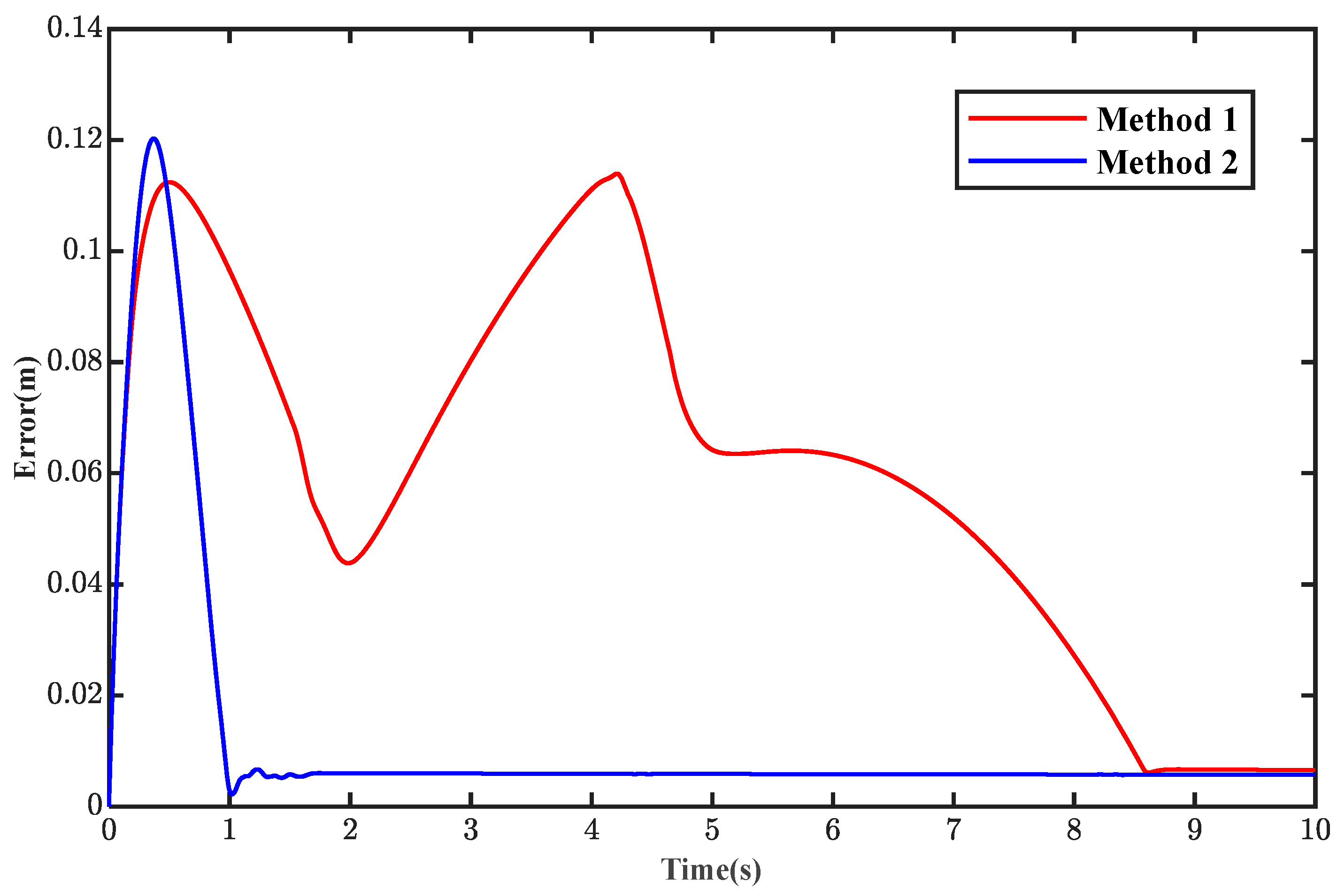
As can be seen from Figure 10 and Figure 11, when the AUV carries out trajectory tracking tasks, after incorporating continuous uncertain ocean current disturbances, Method 2 has stronger anti-interference capabilities compared to Method 1. In the initial stage, the deviation from the reference trajectory is smaller, and it can track the reference trajectory quickly within a short period. However, the actual running trajectory of Method 1 has obvious fluctuations and a lower anti-interference ability. As seen from Figure 12 and Figure 13, after being affected by disturbances, Method 2 can converge the tracking error to zero at a faster speed. As per

Table 5. Position tracking error results with disturbance.

Method	Mean Absolute Error (MAE)	Root Mean Square Error (RMSE)
Method 1	0.079	0.174
Method 2	0.045	0.110

, the Mean Absolute Error of position in Method 2 is only 0.045, which is 43.04% less than that of Method 1. This indicates higher trajectory tracking accuracy and stronger robustness in Method 2. Figure 14 shows the actual control force and torque variation curves under disturbance conditions, the output curve of Method 2 is comparatively smoother.

5. Conclusions

Addressing the issue of 3-D trajectory tracking control for over-actuated underwater robots, a novel tracking control method was herein designed by drawing on the principles of cascade control theory. This involved the use of MPC and the P-S-VUD FLC for the design of kinematic and dynamic controllers, respectively, as well as employing Lyapunov functions to analyze the stability of the outer loop. The modeling process takes into account the spatial arrangement model of the thrusters in over-actuated AUVs, using a direct logic method close to optimal energy consumption for thrust allocation. In designing the kinematic controller, constraints on the linear and angular velocities of the actual model are considered, and control increment input is introduced to reduce errors caused by the linearized kinematic model. The dynamic controller incorporates integral action to enhance system tracking precision and strengthen the system’s resistance to uncertain wave disturbances. Simulation results show that the over-actuated AUV can still achieve fast and precise tracking of 3-D curvilinear trajectories in the presence of continuous uncertain ocean current disturbances, verifying the effectiveness of the designed dual closed-loop controller.

In the future, we will consider using mathematical tools to prove the stability of the inner loop and attempt to implement the proposed design method in a physical over-actuated AUV to enhance its practicality in engineering applications.

References

- Yoerger, D.R.; Jakuba, M.; Bradley, A.M.; Bingham, B. Techniques for deep sea near bottom survey using an autonomous underwater vehicle. In Robotics Research, Proceedings of the 12th International Symposium ISRR, San Francisco, CA, USA, 12–15 October 2005; Springer: Berlin/Heidelberg, Germany, 2007; pp. 416–429. [Google Scholar]
- Stansfield, K.; Smeed, D.A.; Gasparini, G.P.; Mcphail, S.; Millard, N.; Stevenson, P.; Webb, A.; Vetrano, A.; Rabe, B. Deep-sea, high-resolution, hydrography and current measurements using an autonomous underwater vehicle: The overflow from the Strait of Sicily. Geophys. Res. Lett. 2001, 28, 2645–2648. [Google Scholar] [CrossRef]
- Tanakitkorn, K.; Wilson, P.A.; Turnock, S.R.; Phillips, A.B. Depth control for an over-actuated, hover-capable autonomous underwater vehicle with experimental verification. Mechatronics 2017, 41, 67–81. [Google Scholar] [CrossRef]
- Yuan, C.; Shuai, C.; Ma, J.; Fang, Y.; Jiang, S.; Gao, C. Adaptive optimal 3D nonlinear compound line-of-sight trajectory tracking control for over-actuated AUVs in attitude space. Ocean Eng. 2023, 274, 114056. [Google Scholar] [CrossRef]
- Yuan, C.; Shuai, C.; Ma, J.; Fang, Y. An efficient control allocation algorithm for over-actuated AUVs trajectory tracking with fault-tolerant control. Ocean Eng. 2023, 273, 113976. [Google Scholar] [CrossRef]
- Aguiar, A.P.; Hespanha, J.P. Trajectory-tracking and path-following of underactuated autonomous vehicles with parametric modeling uncertainty. IEEE Trans. Autom. Control 2007, 52, 1362–1379. [Google Scholar] [CrossRef]
- Tijjani, A.S.; Chemori, A.; Creuze, V. A survey on tracking control of unmanned underwater vehicles: Experiments-based approach. Annu. Rev. Control 2022, 54, 125–147. [Google Scholar] [CrossRef]
- Wang, L.; Zhu, D.; Pang, W.; Zhang, Y. A survey of underwater search for multi-target using Multi-AUV: Task allocation, path planning, and formation control. Ocean Eng. 2023, 278, 114393. [Google Scholar] [CrossRef]
- Li, Y.; Jiang, Y.; Wang, L.; Cao, J.; Zhang, G. Intelligent PID guidance control for AUV path tracking. J. Cent. South Univ. 2015, 22, 3440–3449. [Google Scholar] [CrossRef]
- Jia, H.-M.; Cheng, X.-Q.; Zhang, L.-J.; Bian, X.; Yan, Z. Three-dimensional path tracking control for underactuated AUV based on adaptive Backstepping. Control Decis. 2012, 27, 652–658. [Google Scholar]
- Liang, X.; Wan, L.; Blake, J.I.; Shenoi, R.A.; Townsend, N. Path following of an underactuated AUV based on fuzzy backstepping sliding mode control. Int. J. Adv. Robot. Syst. 2016, 13, 122. [Google Scholar] [CrossRef]
- Huang, B.; Zhou, B.; Zhang, S.; Zhu, C. Adaptive prescribed performance tracking control for underactuated autonomous underwater vehicles with input quantization. Ocean Eng. 2021, 221, 108549. [Google Scholar] [CrossRef]
- Zhou, H.Y.; Feng, L.X.S. State feedback sliding mode control without chattering by constructing Hurwitz matrix for AUV movement. Int. J. Autom. Comput. 2011, 8, 262–268. [Google Scholar] [CrossRef]
- Gao, F.; Pan, C.; Han, Y. Design and analysis of a new AUV’s sliding control system based on dynamic boundary layer. Chin. J. Mech. Eng. 2013, 26, 35–45. [Google Scholar] [CrossRef]
- Steenson, L.V.; Phillips, A.B.; Rogers, E.; Furlong, M.E.; Turnock, S.R. Experimental Verification of a Depth Controller using Model Predictive Control with Constraints onboard a Thruster Actuated AUV. IFAC Proc. Vol. 2012, 45, 275–280. [Google Scholar] [CrossRef]
- Zhang, G.; Yan, W.; Gao, J. Straight Line Tracking of Underactuacted AUV Based on Model Predictive Control. J. Unmanned Undersea Syst. 2017, 25, 82–88. [Google Scholar]
- Shen, C.; Shi, Y.; Buckham, B. Path-following control of an AUV using multi-objective model predictive control. In Proceedings of the 2016 American Control Conference (ACC), Boston, MA, USA, 6–8 July 2016. [Google Scholar]
- Yao, X.; Wang, X. Path following and obstacle avoidance control of AUV based on MPC guidance law. J. Beijing Univ. Aeronaut. Astronaut. 2020, 46, 1053–1062. [Google Scholar]
- Zhang, Y.; Liu, X.; Luo, M.; Yang, C. MPC-based 3-D trajectory tracking for an autonomous underwater vehicle with constraints in complex ocean environments. Ocean Eng. 2019, 189, 106309. [Google Scholar] [CrossRef]
- Wang, W.; Yan, J.; Wang, H.; Ge, H.; Zhu, Z.; Yang, G. Adaptive MPC trajectory tracking for AUV based on Laguerre function. Ocean Eng. 2022, 261, 111870. [Google Scholar] [CrossRef]
- Yan, Z.; Gong, P.; Zhang, W.; Wu, W. Model predictive control of autonomous underwater vehicles for trajectory tracking with external disturbances. Ocean Eng. 2020, 217, 107884. [Google Scholar] [CrossRef]
- Rashidi, A.J.; Karimi, B.; Khodaparast, A. A constrained predictive controller for AUV and computational optimization using laguerre functions in unknown environments. Int. J. Control Autom. Syst. 2020, 18, 753–767. [Google Scholar] [CrossRef]
- Long, Z.Q.; Liang, X.M.; Yan, G. Universal approximation properties of fuzzy controllers with variable universe of discourse and their approximation conditions. J. Cent. South Univ. (Sci. Technol.) 2012, 43, 3046–3052. [Google Scholar]
- Pham, D.-A.; Han, S.-H. Design of combined neural network and fuzzy logic controller for marine rescue drone trajectory-tracking. J. Mar. Sci. Eng. 2022, 10, 1716. [Google Scholar] [CrossRef]
- Pham, D.-A.; Han, S.-H. Designing a Ship Autopilot System for Operation in a Disturbed Environment Using the Adaptive Neural Fuzzy Inference System. J. Mar. Sci. Eng. 2023, 11, 1262. [Google Scholar] [CrossRef]
- Li, H. To see the success of fuzzy logic from mathematical essence of fuzzy control. Fuzzy Syst. Math. 1995, 9, 1–14. [Google Scholar]
- Jiang, C.; Wan, L.; Zhang, H.; Tang, J.; Wang, J.; Li, S.; Chen, L.; Wu, G.; He, B. A LSSVR Interactive Network for AUV Motion Control. J. Mar. Sci. Eng. 2023, 11, 1111. [Google Scholar] [CrossRef]
- He, Y.; Xie, Y.; Pan, G.; Cao, Y.; Huang, Q.; Ma, S.; Zhang, D.; Cao, Y. Depth and heading control of a manta robot based on S-plane control. J. Mar. Sci. Eng. 2022, 10, 1698. [Google Scholar] [CrossRef]
- Jiang, C.; Lv, J.; Wan, L.; Wang, J.; He, B.; Wu, G. An Improved S-Plane Controller for High-Speed Multi-Purpose AUVs with Situational Static Loads. J. Mar. Sci. Eng. 2023, 11, 646. [Google Scholar] [CrossRef]
- Wang, G.; Yang, Y.; Wang, S. Adaptive digital disturbance rejection controller design for underwater thermal vehicles. J. Mar. Sci. Eng. 2021, 9, 406. [Google Scholar] [CrossRef]
- Perez, T.; Smogeli, O.; Fossen, T.; Sorensen, A.J. An overview of the marine systems simulator (MSS): A simulink toolbox for marine control systems. Model. Identif. Control 2006, 27, 259–275. [Google Scholar] [CrossRef]
- Miller, L.; Brizzolara, S.; Stilwell, D.J. Increase in stability of an x-configured auv through hydrodynamic design iterations with the definition of a new stability index to include effect of gravity. J. Mar. Sci. Eng. 2021, 9, 942. [Google Scholar] [CrossRef]
- Hong, L.; Fang, R.; Cai, X.; Wang, X. Numerical investigation on hydrodynamic performance of a portable AUV. J. Mar. Sci. Eng. 2021, 9, 812. [Google Scholar] [CrossRef]
- Ji, D.; Wang, R.; Zhai, Y.; Gu, H. Dynamic modeling of quadrotor AUV using a novel CFD simulation. Ocean Eng. 2021, 237, 109651. [Google Scholar] [CrossRef]
- Zhu, Y.; Pan, M.; Zhou, W.; Huang, J. Intelligent direct thrust control for multivariable turbofan engine based on reinforcement and deep learning methods. Aerosp. Sci. Technol. 2022, 131, 107972. [Google Scholar] [CrossRef]
- Li, X.; Yang, L. Nonlinear fault-accommodation thrust allocation for over-activated vessels using artificial neural network and multivariate analysis. Ocean Eng. 2022, 266, 112936. [Google Scholar]
- Lang, X.; de Ruiter, A. Distributed optimal control allocation for 6-dof spacecraft with redundant thrusters. Aerosp. Sci. Technol. 2021, 118, 106971. [Google Scholar] [CrossRef]
- Li, H.; Miao, Z.; Wang, J. Variable universe adaptive fuzzy control on the quadruple inverted pendulum. Sci. China E Ser. 2002, 45, 213–224. [Google Scholar] [CrossRef]
- Li, H. Adaptive fuzzy controllers based on variable universe. Sci. China Technol. Sci. 1999, 42, 10–20. [Google Scholar] [CrossRef]
- Liu, Z.L.; Su, C.Y.; Svoboda, J. Control of wing rock phenomenon with a variable universe fuzzy controller. In Proceedings of the 2004 American Control Conference, Boston, MA, USA, 30 June–2 July 2004. [Google Scholar]
- Wu, J.; Han, J.; Yin, Y.; Chen, G. Variable universe based fuzzy control system design for AUV. In Proceedings of the OCEANS 2016-Shanghai, Shanghai, China, 10–13 April 2016; IEEE: Piscataway, NJ, USA, 2016. [Google Scholar]
- Safari, F.; Rafeeyan, M.; Danesh, M. Estimation of hydrodynamic coefficients and simplification of the depth model of an AUV using CFD and sensitivity analysis. Ocean Eng. 2022, 263, 112369. [Google Scholar] [CrossRef]
Figure 1.
The body coordinate system and the inertial coordinate system of the “SZ-1” AUV.
Figure 2.
Propeller space layout of the “SZ-1” AUV. (a) Overhead Layout of the “SZ-1” AUV’s horizontal propellers. (b) Layout of the “SZ-1” AUV’s vertical propellers.
Figure 3.
Control design block diagram of the “SZ-1” AUV.
Figure 4.
Control design diagram of the P-S-VUD FLC.
Figure 5.
The 3-D curve tracking effects without disturbance.
Figure 6.
Position tracking effect on the , , and axes without disturbance.
Figure 7.
Position tracking error curves without disturbance.
Figure 8.
Pitch angle and course angle tracking error curves without disturbance.
Figure 9.
Variation curves of force and torque experienced by the AUV without disturbance.
Figure 10.
The 3-D curve tracking effects with disturbance.
Figure 11.
Position tracking effect on the , , and axes with disturbance.
Figure 12.
Position tracking error curves with disturbance.
Figure 13.
Pitch angle and course angle tracking error curves with disturbance.
Figure 14.
Variation curves of force and torque experienced by the AUV with disturbance.